Rowmotion Markov Chains

Abstract.

Rowmotion is a certain well-studied bijective operator on the distributive lattice $J(P)$ of order ideals of a finite poset $P$. We introduce the rowmotion Markov chain ${\bf M}_{J(P)}$ by assigning a probability $p_{x}$ to each $x\in P$ and using these probabilities to insert randomness into the original definition of rowmotion. More generally, we introduce a very broad family of toggle Markov chains inspired by Striker’s notion of generalized toggling. We characterize when toggle Markov chains are irreducible, and we show that each toggle Markov chain has a remarkably simple stationary distribution.

We also provide a second generalization of rowmotion Markov chains to the context of semidistrim lattices. Given a semidistrim lattice $L$, we assign a probability $p_{j}$ to each join-irreducible element $j$ of $L$ and use these probabilities to construct a rowmotion Markov chain ${\bf M}_{L}$. Under the assumption that each probability $p_{j}$ is strictly between $0$ and $1$, we prove that ${\bf M}_{L}$ is irreducible. We also compute the stationary distribution of the rowmotion Markov chain of a lattice obtained by adding a minimal element and a maximal element to a disjoint union of two chains.

We bound the mixing time of ${\bf M}_{L}$ for an arbitrary semidistrim lattice $L$. In the special case when $L$ is a Boolean lattice, we use spectral methods to obtain much stronger estimates on the mixing time, showing that rowmotion Markov chains of Boolean lattices exhibit the cutoff phenomenon.

1. Introduction

1.1. Distributive Lattices

Let $P$ be a finite poset, and let $J(P)$ denote the set of order ideals (i.e., down-sets) of $P$. For $S\subseteq P$, let

$$\Delta(S)=\{x\in P:x\leq s\text{ for some }s\in S\}\quad\text{and}\quad\nabla(S)=\{x\in P:x\geq s\text{ for some }s\in S\},$$

and let $\min(S)$ and $\max(S)$ denote the set of minimal elements and the set of maximal elements of $S$, respectively. Rowmotion, a well-studied operator in the growing field of dynamical algebraic combinatorics, is the bijection $\mathrm{Row}\colon J(P)\to J(P)$ defined by

(1) $$\mathrm{Row}(I)=P\setminus\nabla(\max(I)).$$

We refer the reader to [20, 22] for the history of rowmotion. The purpose of this article is to introduce randomness into the ongoing saga of rowmotion by defining certain Markov chains. We were inspired by the articles [1, 15, 18]; these articles define Markov chains based on the promotion operator, which is closely related to rowmotion in special cases [4, 20] (though our Markov chains are fundamentally different from these promotion-based Markov chains).

For each $x\in P$, fix a probability $p_{x}\in[0,1]$. We define the rowmotion Markov chain ${\bf M}_{J(P)}$ with state space $J(P)$ as follows. Starting from a state $I\in J(P)$, select a random subset $S$ of $\max(I)$ by adding each element $x\in\max(I)$ into $S$ with probability $p_{x}$; then transition to the new state $P\setminus\nabla(S)=\mathrm{Row}(\Delta(S))$. Thus, for any $I,I^{\prime}\in J(P)$, the transition probability from $I$ to $I^{\prime}$ is

$$\mathbb{P}(I\to I^{\prime})=\begin{cases}\left(\prod\limits_{x\in\min(P\setminus I^{\prime})}p_{x}\right)\left(\prod\limits_{x^{\prime}\in\max(I)\setminus\min(P\setminus I^{\prime})}(1-p_{x^{\prime}})\right)&\mbox{if }\min(P\setminus I^{\prime})\subseteq\max(I);\\ 0&\mbox{otherwise.}\end{cases}$$

Observe that if $p_{x}=1$ for all $x\in P$, then ${\bf M}_{J(P)}$ is deterministic and agrees with the rowmotion operator. On the other hand, if $p_{x}=0$ for all $x\in P$, then ${\bf M}_{J(P)}$ is deterministic and sends every order ideal of $P$ to the order ideal $P$.

Example 1.1.

Suppose $P$ is the poset

$$\begin{array}[]{l}\includegraphics[height=25.6073pt]{RowmotionMarkovPIC2}\end{array},$$

whose elements $x,y,z$ are as indicated. Then $J(P)$ forms a distributive lattice with $5$ elements. The transition diagram of ${\bf M}_{J(P)}$ is drawn over the Hasse diagram of $J(P)$ in Figure 1.

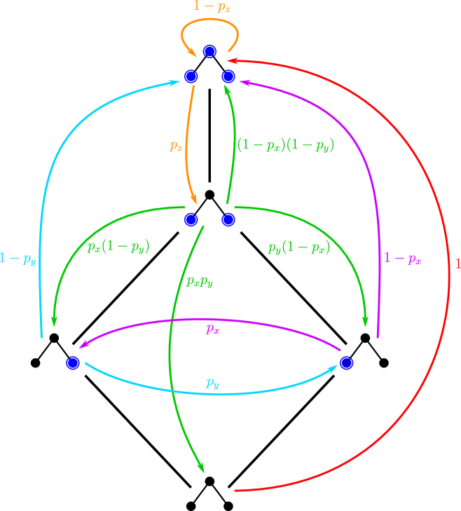
Figure 1. The transition diagram of ${\bf M}_{J(P)}$, where $P$ is the $3$-element poset from Example 1.1. The elements of each order ideal in $J(P)$ are circled and blue.

Suppose each probability $p_{x}$ is strictly between 0 and 1. One of our main results will imply that ${\bf M}_{J(P)}$ is irreducible and that the probability of the state $I$ in the stationary distribution of ${\bf M}_{J(P)}$ is

(2) $$\frac{1}{Z(J(P))}\prod_{x\in I}p_{x}^{-1},$$

where $\displaystyle Z(J(P))=\sum_{I^{\prime}\in J(P)}\prod_{x^{\prime}\in I^{\prime}}p_{x^{\prime}}^{-1}$.

It is surprising that there is such a clean formula for the stationary distribution in this level of generality. We will deduce this result from a more general result about a vastly broader family of Markov chains.

1.2. Toggle Markov Chains

Let $P$ be a finite set of size $n$, and let $\mathcal{K}$ be a collection of subsets of $P$. For each $x\in P$, define the toggle operator $\tau_{x}\colon\mathcal{K}\to\mathcal{K}$ by

$$\tau_{x}(A)=\begin{cases}A\triangle\{x\}&\text{ if }A\triangle\{x\}\in\mathcal{K}\\ A&\text{ otherwise},\end{cases}$$

where $\triangle$ denotes symmetric difference. Note that $\tau_{x}$ is an involution. Fix a tuple ${\bf x}=(x_{1},\ldots,x_{n})$ that contains each element of $P$ exactly once. In other words, ${\bf x}$ is an ordering of the elements of $P$. Given a set $Y\subseteq P$, let $\tau_{Y}=\tau_{y_{r}}\circ\cdots\circ\tau_{y_{1}}$, where $y_{1},\ldots,y_{r}$ is the list of elements of $Y$ in the order that they appear within the list $x_{1},\ldots,x_{n}$.

Striker [19] viewed the map $\tau_{P}\colon\mathcal{K}\to\mathcal{K}$ as a generalization of rowmotion. Indeed, if $P$ is a poset, ${\bf x}=(x_{1},\ldots,x_{n})$ is a linear extension of $P$ (meaning $i<j$ whenever $x_{i}<x_{j}$ in $P$), and $\mathcal{K}=J(P)$, then $\tau_{P}$ is equal to rowmotion. The recent article [10] studies the dynamical aspects of $\tau_{P}$ when $P$ is a poset, ${\bf x}$ is a linear extension of $P$, and $\mathcal{K}$ is the collection of interval-closed (also called convex) subsets of $P$. The articles [6, 12, 13] consider $\tau_{P}$ when $P$ is the vertex set of a particular graph, ${\bf x}$ is a special ordering of the vertices, and $\mathcal{K}$ is the collection of independent sets of the graph.

For each $x\in P$, fix a probability $p_{x}$. Define the toggle Markov chain $\mathbf{T}=\mathbf{T}(\mathcal{K},{\bf x})$ as follows. The state space of $\mathbf{T}$ is $\mathcal{K}$. Suppose the Markov chain is in a state $A\in\mathcal{K}$. Choose a subset $T\subseteq A$ randomly so that each element $x\in A$ is included in $T$ with probability $p_{x}$, and then transition from $A$ to the new state $\tau_{T}(A)$.

To phrase this differently, define the random toggle $\widetilde{\tau}_{x}$ to be the stochastic operator that acts as follows on a set $A\in\mathcal{K}$. Let $X$ be a Bernoulli random variable that takes the value $1$ with probability $p_{x}$, and let

$$\widetilde{\tau}_{x}(A)=\begin{cases}\tau_{x}(A)&\mbox{if }x\not\in A\text{ or }X=1;\\ A&\mbox{if }x\in A\text{ and }X=0.\end{cases}$$

Then the Markov chain transitions from the state obtained from $A$ by applying the random toggles $\widetilde{\tau}_{x_{1}},\ldots,\widetilde{\tau}_{x_{n}}$ in this order. (Each time we apply a random toggle, we use a new Bernoulli random variable that is independent of those used before.)

Example 1.2.

Suppose $G$ is the graph

$$\begin{array}[]{l}\includegraphics[height=15.67732pt]{RowmotionMarkovPIC8}\end{array},$$

whose vertices $x,y,z$ are as indicated. Let $\mathcal{K}$ be the collection of independent sets of $G$. Figure 2 depicts the random toggles $\widetilde{\tau}_{x},\widetilde{\tau}_{y},\widetilde{\tau}_{z}$. If we let ${\bf x}=(x,y,z)$, then a transition of ${\bf T}(\mathcal{K},{\bf x})$ consists of applying these random toggles in the order $\widetilde{\tau}_{x},\widetilde{\tau}_{y},\widetilde{\tau}_{z}$.

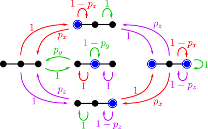
Figure 2. As in Example 1.2, we consider random toggles, where $\mathcal{K}$ is the collection of independent sets of a path graph with vertices $x,y,z$ (from left to right). The elements of each independent set are circled and blue. To apply the random toggle $\widetilde{\tau}_{x}$ to an independent set $A$, we follow one of the red arrows starting at $A$; the probability that a particular arrow is used is written next to the arrow. Similarly, we follow a green arrow when we apply $\widetilde{\tau}_{y}$, and we follow a purple arrow when we apply $\widetilde{\tau}_{z}$.

Given a set $P$, let $\mathcal{H}^{P}$ be the hypercube graph with vertex set $2^{P}$ (the power set of $P$) such that two sets $A,A^{\prime}\subseteq P$ are adjacent if and only if $|A\triangle A^{\prime}|=1$. For $S\subseteq 2^{P}$, let $\mathcal{H}^{P}|_{S}$ be the induced subgraph of $\mathcal{H}^{P}$ with vertex set $S$.

Let us now state our main results about irreducibility and stationary distributions of toggle Markov chains. As before, we fix a finite set $P$, a collection $\mathcal{K}$ of subsets of $P$, an ordering ${\bf x}$ of the elements of $P$, and a probability $p_{x}$ for each $x\in P$.

Theorem 1.3.

Suppose $0<p_{x}<1$ for each $x\in P$. The toggle Markov chain $\mathbf{T}(\mathcal{K},{\bf x})$ is irreducible if and only if the graph $\mathcal{H}^{P}|_{\mathcal{K}}$ is connected.

If $P$ is a finite poset, then every connected component of $\mathcal{H}^{P}_{J(P)}$ contains the empty set as a vertex. Thus, it is immediate from Theorem 1.3 that the rowmotion Markov chain ${\bf M}_{J(P)}$ is irreducible whenever $0<p_{x}<1$ for every $x\in P$.

Theorem 1.4.

Suppose that the toggle Markov chain $\mathbf{T}(\mathcal{K},{\bf x})$ is irreducible and that $p_{x}>0$ for every $x\in P$. For $A\in\mathcal{K}$, the probability of the state $A$ in the stationary distribution of $\mathbf{T}(\mathcal{K},{\bf x})$ is

$$\frac{1}{Z(\mathcal{K})}\prod_{x\in A}p_{x}^{-1},$$

where $\displaystyle Z(\mathcal{K})=\sum_{A^{\prime}\in\mathcal{K}}\prod_{x^{\prime}\in A^{\prime}}p_{x^{\prime}}^{-1}$.

Note that the stationary distribution in Theorem 1.4 is independent of the ordering ${\bf x}$ (though the Markov chain itself can certainly depend on ${\bf x}$).

1.3. Mixing Times

Suppose ${\bf M}$ is an irreducible finite Markov chain with state space $\Omega$, transition matrix $Q$, and stationary distribution $\pi$. For $x\in\Omega$, let $Q^{i}(x,\cdot)$ denote the distribution on $\Omega$ in which the probability of a state $x^{\prime}$ is the probability of reaching $x^{\prime}$ by starting at $x$ and applying $i$ transitions (this probability is the entry in $Q^{i}$ in the row indexed by $x$ and the column indexed by $x^{\prime}$). In other words, $Q^{i}(x,\cdot)$ is the law on $\Omega$ after $i$ steps of the Markov chain, starting at $x$. The total variation distance $d_{\mathrm{TV}}=d_{\mathrm{TV}}^{\Omega}$ is the metric on the space of distributions on $\Omega$ defined by

$$d_{\mathrm{TV}}(\mu,\nu)=\max_{A\subseteq\Omega}|\mu(A)-\nu(A)|=\frac{1}{2}\sum_{x\in\Omega}|\mu(x)-\nu(x)|.$$

For $\varepsilon>0$, the mixing time of ${\bf M}$, denoted $t^{\mathrm{mix}}_{{\bf M}}(\varepsilon)$, is the smallest nonnegative integer $i$ such that $d_{\mathrm{TV}}(Q^{i}(x,\cdot),\pi)<\varepsilon$ for all $x\in\Omega$.

The width of a finite poset $P$, denoted $0pt(P)$, is the maximum size of an antichain in $P$. In Section 5, we use the method of coupling to prove the following bound on the mixing time of an arbitrary rowmotion Markov chain.

Theorem 1.5.

Let $P$ be a finite poset, and fix a probability $p_{x}\in(0,1)$ for each $x\in P$. Let $\overline{p}=\max\limits_{x\in P}p_{x}$. For each $\varepsilon>0$, the mixing time of ${\bf M}_{J(P)}$ satisfies

$$t^{\mathrm{mix}}_{{\bf M}_{J(P)}}(\varepsilon)\leq\left\lceil\frac{\log\varepsilon}{\log\left(1-\left(1-\overline{p}\right)^{0pt(P)}\right)}\right\rceil.$$

We can drastically improve the bound in Theorem 1.5 when $P$ is an antichain (so $J(P)$ is a Boolean lattice). For simplicity, we assume that all probabilities $p_{x}$ are equal to a single value $p$. In this setting, the Markov chain is reversible with respect to $\pi$; this allows us to give a spectral proof of the following result, which is an instance of the well-studied cutoff phenomenon. (See [14, Chapter 18] for a discussion of cutoff.)

Theorem 1.6.

Let $P$ be an $n$-element antichain, and fix a probability $p\in(0,1)$. Let $p_{x}=p$ for all $x\in P$. Let $Q$ and $\pi$ be the transition matrix and stationary distribution, respectively, of the Markov chain ${\bf M}_{J(P)}$.

1. For $c>\frac{1}{2}$ and $t=\frac{1}{2}\log_{1/p}n+c$, we have

   $$\max_{x\in J(P)}d_{\mathrm{TV}}(Q^{t}(x,\cdot),\pi)\leq\frac{1}{2}\left(e^{p^{2c-1}}-1\right)^{1/2}.$$

2. For $0<c<\frac{1}{2}\log_{1/p}n$ and $t=\frac{1}{2}\log_{1/p}n-c$, we have

   $$\max_{x\in J(P)}d_{\mathrm{TV}}(Q^{t}(x,\cdot),\pi)\geq 1-4p^{2c+1}-4p^{2c}.$$

It would be interesting to prove that other natural families of toggle Markov chains exhibit cutoff.

1.4. Semidistrim Lattices

If $P$ is a finite poset, then we can order $J(P)$ by inclusion to obtain a distributive lattice. In fact, Birkhoff’s Fundamental Theorem of Finite Distributive Lattices [5] states that every finite distributive lattice is isomorphic to the lattice of order ideals of some finite poset. Thus, instead of viewing rowmotion as a bijective operator on the set of order ideals of a finite poset, one can equivalently view it as a bijective operator on the set of elements of a distributive lattice. This perspective has led to more general definitions of rowmotion in recent years. Barnard [2] showed how to extend the definition of rowmotion to the broader family of semidistributive lattices, while Thomas and Williams [22] discussed how to extend the definition to the family of trim lattices. (Every distributive lattice is semidistributive and trim, but there are semidistributive lattices that are not trim and trim lattices that are not semidistributive.)

One notable example motivating these extended definitions comes from Reading’s Cambrian lattices [16]. Suppose $c$ is a Coxeter element of a finite Coxeter group $W$. Reading [17] found a bijection from the $c$-Cambrian lattice to the $c$-noncrossing partition lattice of $W$; under this bijection, rowmotion on the $c$-Cambrian lattice corresponds to the well-studied Kreweras complementation operator on the $c$-noncrossing partition lattice of $W$ [2, 22]. See [8, 11, 22] for other non-distributive lattices where rowmotion has been studied.

Recently, the first author and Williams [9] introduced the even broader family of semidistrim lattices and showed how to define a natural rowmotion operator on them; this is now the broadest family of lattices where rowmotion has been defined. It turns out that we can extend our definition of rowmotion Markov chains to semidistrim lattices; this provides a generalization of rowmotion Markov chains that is different from the toggle Markov chains discussed in Section 1.2. Let us sketch the details here and wait until Section 4 to define semidistrim lattices properly and explain why this definition specializes to the one given above when the lattice is distributive.

Let $L$ be a semidistrim lattice, and let $\mathcal{J}_{L}$ and $\mathcal{M}_{L}$ be the set of join-irreducible elements of $L$ and the set of meet-irreducible elements of $L$, respectively. There is a specific bijection $\kappa_{L}\colon\mathcal{J}_{L}\to\mathcal{M}_{L}$ satisfying certain properties. The Galois graph of $L$ is the loopless directed graph $G_{L}$ with vertex set $\mathcal{J}_{L}$ such that for all distinct $j,j^{\prime}\in\mathcal{J}_{L}$, there is an arrow $j\to j^{\prime}$ if and only if $j\not\leq\kappa_{L}(j^{\prime})$. Let $\mathrm{Ind}(G_{L})$ be the set of independent sets of $G_{L}$. There is a particular way to label the edges of the Hasse diagram of $L$ with elements of $\mathcal{J}_{L}$; we write $j_{uv}$ for the label of the edge $u\lessdot v$. For $w\in L$, let $\mathcal{D}_{L}(w)$ be the set of labels of the edges of the form $u\lessdot w$, and let $\mathcal{U}_{L}(w)$ be the set of labels of the edges of the form $w\lessdot v$. Then $\mathcal{D}_{L}(w)$ and $\mathcal{U}_{L}(w)$ are actually independent sets of $G_{L}$. Moreover, the maps $\mathcal{D}_{L},\mathcal{U}_{L}\colon L\to\mathrm{Ind}(G_{L})$ are bijections. The rowmotion operator $\mathrm{Row}\colon L\to L$ is defined by $\mathrm{Row}=\mathcal{U}_{L}^{-1}\circ\mathcal{D}_{L}$.

The rowmotion Markov chain ${\bf M}_{L}$ has $L$ as its set of states. For each $j\in\mathcal{J}_{L}$, we fix a probability $p_{j}\in[0,1]$. Starting at a state $u\in L$, we choose a random subset $S$ of $\mathcal{D}_{L}(u)$ by adding each element $j\in\mathcal{D}_{L}(u)$ into $S$ with probability $p_{j}$ and then transition to the new state $u^{\prime}=\mathrm{Row}_{L}(\bigvee S)$.

When $p_{j}=1$ for all $j\in\mathcal{J}_{L}$, the Markov chain ${\bf M}_{L}$ is deterministic and agrees with rowmotion; indeed, this follows from [9, Theorem 5.6], which tells us that $\bigvee\mathcal{D}_{L}(u)=u$ for all $u\in L$.

Our main result about rowmotion Markov chains of semidistrim lattices is as follows.

Theorem 1.7.

Let $L$ be a semidistrim lattice, and fix a probability $p_{j}\in(0,1)$ for each join-irreducible element $j\in\mathcal{J}_{L}$. The rowmotion Markov chain ${\bf M}_{L}$ is irreducible.

Let us remark that this theorem is not at all obvious. Our proof uses a delicate induction that relies on some difficult results about semidistrim lattices proven in [9]. For example, we use the fact that intervals in semidistrim lattices are semidistrim.

We can also generalize Theorem 1.5 to the realm of semidistrim lattices in the following theorem. Given a semidistrim lattice $L$ and an element $u\in L$, we write $\mathrm{ddeg}(u)$ for the down-degree of $u$, which is the number of elements of $L$ covered by $u$. Let $\alpha(G_{L})$ denote the independence number of the Galois graph $G_{L}$; that is, $\alpha(G_{L})=\max\limits_{\mathcal{I}\in\mathrm{Ind}(G_{L})}|\mathcal{I}|$. Equivalently, $\alpha(G_{L})=\max\limits_{u\in L}\mathrm{ddeg}(u)$. If $P$ is a finite poset, then $\alpha(G_{J(P)})=0pt(P)$.

Theorem 1.8.

Let $L$ be a semidistrim lattice, and fix a probability $p_{j}\in(0,1)$ for each $j\in\mathcal{J}_{L}$. Let $\overline{p}=\max\limits_{j\in\mathcal{J}_{L}}p_{j}$. For each $\varepsilon>0$, the mixing time of ${\bf M}_{L}$ satisfies

$$t^{\mathrm{mix}}_{{\bf M}_{L}}(\varepsilon)\leq\left\lceil\frac{\log\varepsilon}{\log\left(1-\left(1-\overline{p}\right)^{\alpha(G_{L})}\right)}\right\rceil.$$

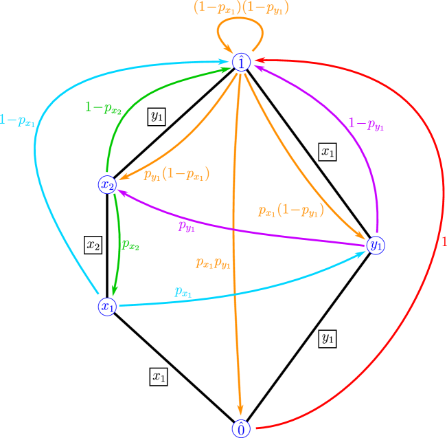
Figure 4. The transition diagram of ${\bf M}_{\text{$\mathchoice{\raisebox{-1.99168pt}{\includegraphics[height=6.63052pt]{hexx}}}{\raisebox{-1.99168pt}{\includegraphics[height=6.63052pt]{hexx}}}{\raisebox{-1.70717pt}{\includegraphics[height=4.82224pt]{hexx}}}{\raisebox{-1.42262pt}{\includegraphics[height=3.01389pt]{hexx}}}$}_{2,1}}$ drawn over the Hasse diagram of $\mathchoice{\raisebox{-1.99168pt}{\includegraphics[height=9.47217pt]{hexx}}}{\raisebox{-1.99168pt}{\includegraphics[height=9.47217pt]{hexx}}}{\raisebox{-1.70717pt}{\includegraphics[height=6.88889pt]{hexx}}}{\raisebox{-1.42262pt}{\includegraphics[height=4.30554pt]{hexx}}}_{2,1}$. Next to each edge $u\lessdot v$ is a box containing the edge label $j_{uv}$.

We were not able to find a formula for the stationary distribution of the rowmotion Markov chain of an arbitrary semidistrim (or even semidistributive or trim) lattice; this serves to underscore the anomalistic nature of the formula for distributive lattices in (2). However, there is one family of semidistrim (in fact, semidistributive) lattices where we were able to find such a formula. Given positive integers $a$ and $b$, let $\mathchoice{\raisebox{-1.99168pt}{\includegraphics[height=9.47217pt]{hexx}}}{\raisebox{-1.99168pt}{\includegraphics[height=9.47217pt]{hexx}}}{\raisebox{-1.70717pt}{\includegraphics[height=6.88889pt]{hexx}}}{\raisebox{-1.42262pt}{\includegraphics[height=4.30554pt]{hexx}}}_{a,b}$ be the lattice obtained by taking two disjoint chains $x_{1}<\cdots<x_{a}$ and $y_{1}<\cdots<y_{b}$ and adding a bottom element $\hat{0}$ and a top element $\hat{1}$. Let us remark that $\mathchoice{\raisebox{-1.99168pt}{\includegraphics[height=9.47217pt]{hexx}}}{\raisebox{-1.99168pt}{\includegraphics[height=9.47217pt]{hexx}}}{\raisebox{-1.70717pt}{\includegraphics[height=6.88889pt]{hexx}}}{\raisebox{-1.42262pt}{\includegraphics[height=4.30554pt]{hexx}}}_{m-1,m-1}$ is isomorphic to the weak order of the dihedral group of order $2m$, whereas $\mathchoice{\raisebox{-1.99168pt}{\includegraphics[height=9.47217pt]{hexx}}}{\raisebox{-1.99168pt}{\includegraphics[height=9.47217pt]{hexx}}}{\raisebox{-1.70717pt}{\includegraphics[height=6.88889pt]{hexx}}}{\raisebox{-1.42262pt}{\includegraphics[height=4.30554pt]{hexx}}}_{m-1,1}$ is isomorphic to the $c$-Cambrian lattice of that same dihedral group (for any Coxeter element $c$). We have $\mathcal{J}_{\mathchoice{\raisebox{-1.99168pt}{\includegraphics[height=6.63052pt]{hexx}}}{\raisebox{-1.99168pt}{\includegraphics[height=6.63052pt]{hexx}}}{\raisebox{-1.70717pt}{\includegraphics[height=4.82224pt]{hexx}}}{\raisebox{-1.42262pt}{\includegraphics[height=3.01389pt]{hexx}}}_{a,b}}=\mathcal{M}_{\mathchoice{\raisebox{-1.99168pt}{\includegraphics[height=6.63052pt]{hexx}}}{\raisebox{-1.99168pt}{\includegraphics[height=6.63052pt]{hexx}}}{\raisebox{-1.70717pt}{\includegraphics[height=4.82224pt]{hexx}}}{\raisebox{-1.42262pt}{\includegraphics[height=3.01389pt]{hexx}}}_{a,b}}=\{x_{1},\ldots,x_{a},y_{1},\ldots,y_{b}\}$. For $2\leq i\leq a$ and $2\leq i^{\prime}\leq b$, we have $\kappa_{\mathchoice{\raisebox{-1.99168pt}{\includegraphics[height=6.63052pt]{hexx}}}{\raisebox{-1.99168pt}{\includegraphics[height=6.63052pt]{hexx}}}{\raisebox{-1.70717pt}{\includegraphics[height=4.82224pt]{hexx}}}{\raisebox{-1.42262pt}{\includegraphics[height=3.01389pt]{hexx}}}_{a,b}}(x_{i})=x_{i-1}$ and $\kappa_{\mathchoice{\raisebox{-1.99168pt}{\includegraphics[height=6.63052pt]{hexx}}}{\raisebox{-1.99168pt}{\includegraphics[height=6.63052pt]{hexx}}}{\raisebox{-1.70717pt}{\includegraphics[height=4.82224pt]{hexx}}}{\raisebox{-1.42262pt}{\includegraphics[height=3.01389pt]{hexx}}}_{a,b}}(y_{i^{\prime}})=y_{i^{\prime}-1}$; moreover, $\kappa_{\mathchoice{\raisebox{-1.99168pt}{\includegraphics[height=6.63052pt]{hexx}}}{\raisebox{-1.99168pt}{\includegraphics[height=6.63052pt]{hexx}}}{\raisebox{-1.70717pt}{\includegraphics[height=4.82224pt]{hexx}}}{\raisebox{-1.42262pt}{\includegraphics[height=3.01389pt]{hexx}}}_{a,b}}(x_{1})=y_{b}$ and $\kappa_{\mathchoice{\raisebox{-1.99168pt}{\includegraphics[height=6.63052pt]{hexx}}}{\raisebox{-1.99168pt}{\includegraphics[height=6.63052pt]{hexx}}}{\raisebox{-1.70717pt}{\includegraphics[height=4.82224pt]{hexx}}}{\raisebox{-1.42262pt}{\includegraphics[height=3.01389pt]{hexx}}}_{a,b}}(y_{1})=x_{a}$. This is illustrated in Figure 3 when $a=3$ and $b=2$. Figure 4 shows the transition diagram of ${\bf M}_{\text{$\mathchoice{\raisebox{-1.99168pt}{\includegraphics[height=6.63052pt]{hexx}}}{\raisebox{-1.99168pt}{\includegraphics[height=6.63052pt]{hexx}}}{\raisebox{-1.70717pt}{\includegraphics[height=4.82224pt]{hexx}}}{\raisebox{-1.42262pt}{\includegraphics[height=3.01389pt]{hexx}}}$}_{2,1}}$.

Figure 3. The lattice $\mathchoice{\raisebox{-1.99168pt}{\includegraphics[height=9.47217pt]{hexx}}}{\raisebox{-1.99168pt}{\includegraphics[height=9.47217pt]{hexx}}}{\raisebox{-1.70717pt}{\includegraphics[height=6.88889pt]{hexx}}}{\raisebox{-1.42262pt}{\includegraphics[height=4.30554pt]{hexx}}}_{3,2}$. Next to each edge $u\lessdot v$ is a box containing the edge label $j_{uv}$. The red arrows represent the action of $\kappa_{\mathchoice{\raisebox{-1.99168pt}{\includegraphics[height=6.63052pt]{hexx}}}{\raisebox{-1.99168pt}{\includegraphics[height=6.63052pt]{hexx}}}{\raisebox{-1.70717pt}{\includegraphics[height=4.82224pt]{hexx}}}{\raisebox{-1.42262pt}{\includegraphics[height=3.01389pt]{hexx}}}_{3,2}}$.

Theorem 1.9.

Fix positive integers $a$ and $b$, and let $\kappa=\kappa_{\mathchoice{\raisebox{-1.99168pt}{\includegraphics[height=6.63052pt]{hexx}}}{\raisebox{-1.99168pt}{\includegraphics[height=6.63052pt]{hexx}}}{\raisebox{-1.70717pt}{\includegraphics[height=4.82224pt]{hexx}}}{\raisebox{-1.42262pt}{\includegraphics[height=3.01389pt]{hexx}}}_{a,b}}$. For each $j\in\mathcal{J}_{\text{$\mathchoice{\raisebox{-1.99168pt}{\includegraphics[height=6.63052pt]{hexx}}}{\raisebox{-1.99168pt}{\includegraphics[height=6.63052pt]{hexx}}}{\raisebox{-1.70717pt}{\includegraphics[height=4.82224pt]{hexx}}}{\raisebox{-1.42262pt}{\includegraphics[height=3.01389pt]{hexx}}}$}_{a,b}}$, fix a probability $p_{j}\in(0,1)$. There is a constant $Z(\mathchoice{\raisebox{-1.99168pt}{\includegraphics[height=9.47217pt]{hexx}}}{\raisebox{-1.99168pt}{\includegraphics[height=9.47217pt]{hexx}}}{\raisebox{-1.70717pt}{\includegraphics[height=6.88889pt]{hexx}}}{\raisebox{-1.42262pt}{\includegraphics[height=4.30554pt]{hexx}}}_{a,b})$ (depending only on $a$ and $b$) such that in the stationary distribution of ${\bf M}_{\text{$\mathchoice{\raisebox{-1.99168pt}{\includegraphics[height=6.63052pt]{hexx}}}{\raisebox{-1.99168pt}{\includegraphics[height=6.63052pt]{hexx}}}{\raisebox{-1.70717pt}{\includegraphics[height=4.82224pt]{hexx}}}{\raisebox{-1.42262pt}{\includegraphics[height=3.01389pt]{hexx}}}$}_{a,b}}$, we have

$$\mathbb{P}(\hat{0}) =\frac{1}{Z(\mathchoice{\raisebox{-1.99168pt}{\includegraphics[height=9.47217pt]{hexx}}}{\raisebox{-1.99168pt}{\includegraphics[height=9.47217pt]{hexx}}}{\raisebox{-1.70717pt}{\includegraphics[height=6.88889pt]{hexx}}}{\raisebox{-1.42262pt}{\includegraphics[height=4.30554pt]{hexx}}}_{a,b})}p_{x_{1}}p_{y_{1}}\left(1-\prod_{j\in\mathcal{J}_{\text{$\mathchoice{\raisebox{-1.99168pt}{\includegraphics[height=4.73608pt]{hexx}}}{\raisebox{-1.99168pt}{\includegraphics[height=4.73608pt]{hexx}}}{\raisebox{-1.70717pt}{\includegraphics[height=3.44444pt]{hexx}}}{\raisebox{-1.42262pt}{\includegraphics[height=2.15277pt]{hexx}}}$}_{a,b}}}p_{j}\right);$$

$$\mathbb{P}(\hat{1}) =\frac{1}{Z(\mathchoice{\raisebox{-1.99168pt}{\includegraphics[height=9.47217pt]{hexx}}}{\raisebox{-1.99168pt}{\includegraphics[height=9.47217pt]{hexx}}}{\raisebox{-1.70717pt}{\includegraphics[height=6.88889pt]{hexx}}}{\raisebox{-1.42262pt}{\includegraphics[height=4.30554pt]{hexx}}}_{a,b})}\left(1-\prod_{j\in\mathcal{J}_{\text{$\mathchoice{\raisebox{-1.99168pt}{\includegraphics[height=4.73608pt]{hexx}}}{\raisebox{-1.99168pt}{\includegraphics[height=4.73608pt]{hexx}}}{\raisebox{-1.70717pt}{\includegraphics[height=3.44444pt]{hexx}}}{\raisebox{-1.42262pt}{\includegraphics[height=2.15277pt]{hexx}}}$}_{a,b}}}p_{j}\right);$$

$$\mathbb{P}(x_{i}) =\frac{1}{Z(\text{$\mathchoice{\raisebox{-1.99168pt}{\includegraphics[height=9.47217pt]{hexx}}}{\raisebox{-1.99168pt}{\includegraphics[height=9.47217pt]{hexx}}}{\raisebox{-1.70717pt}{\includegraphics[height=6.88889pt]{hexx}}}{\raisebox{-1.42262pt}{\includegraphics[height=4.30554pt]{hexx}}}$}_{a,b})}\left((1-p_{x_{1}})\prod_{\begin{subarray}{c}j\in\mathcal{J}_{\text{$\mathchoice{\raisebox{-1.99168pt}{\includegraphics[height=4.73608pt]{hexx}}}{\raisebox{-1.99168pt}{\includegraphics[height=4.73608pt]{hexx}}}{\raisebox{-1.70717pt}{\includegraphics[height=3.44444pt]{hexx}}}{\raisebox{-1.42262pt}{\includegraphics[height=2.15277pt]{hexx}}}$}_{a,b}}\\ \kappa(j)\geq x_{i}\end{subarray}}p_{j}+(1-p_{y_{1}})\prod_{\begin{subarray}{c}j\in\mathcal{J}_{\text{$\mathchoice{\raisebox{-1.99168pt}{\includegraphics[height=4.73608pt]{hexx}}}{\raisebox{-1.99168pt}{\includegraphics[height=4.73608pt]{hexx}}}{\raisebox{-1.70717pt}{\includegraphics[height=3.44444pt]{hexx}}}{\raisebox{-1.42262pt}{\includegraphics[height=2.15277pt]{hexx}}}$}_{a,b}}\\ \kappa(j)\not<x_{i}\end{subarray}}p_{j}\right)\quad\text{for}\quad 1\leq i\leq a;$$

$$\mathbb{P}(y_{i}) =\frac{1}{Z(\text{$\mathchoice{\raisebox{-1.99168pt}{\includegraphics[height=9.47217pt]{hexx}}}{\raisebox{-1.99168pt}{\includegraphics[height=9.47217pt]{hexx}}}{\raisebox{-1.70717pt}{\includegraphics[height=6.88889pt]{hexx}}}{\raisebox{-1.42262pt}{\includegraphics[height=4.30554pt]{hexx}}}$}_{a,b})}\left((1-p_{y_{1}})\prod_{\begin{subarray}{c}j\in\mathcal{J}_{\text{$\mathchoice{\raisebox{-1.99168pt}{\includegraphics[height=4.73608pt]{hexx}}}{\raisebox{-1.99168pt}{\includegraphics[height=4.73608pt]{hexx}}}{\raisebox{-1.70717pt}{\includegraphics[height=3.44444pt]{hexx}}}{\raisebox{-1.42262pt}{\includegraphics[height=2.15277pt]{hexx}}}$}_{a,b}}\\ \kappa(j)\geq y_{i}\end{subarray}}p_{j}+(1-p_{x_{1}})\prod_{\begin{subarray}{c}j\in\mathcal{J}_{\text{$\mathchoice{\raisebox{-1.99168pt}{\includegraphics[height=4.73608pt]{hexx}}}{\raisebox{-1.99168pt}{\includegraphics[height=4.73608pt]{hexx}}}{\raisebox{-1.70717pt}{\includegraphics[height=3.44444pt]{hexx}}}{\raisebox{-1.42262pt}{\includegraphics[height=2.15277pt]{hexx}}}$}_{a,b}}\\ \kappa(j)\not<y_{i}\end{subarray}}p_{j}\right)\quad\text{for}\quad 1\leq i\leq b.$$

Section 2 provides preliminary background on Markov chains and posets. In Section 3, we prove Theorems 1.3 and 1.4, which characterize when toggle Markov chains are irreducible and exhibit the stationary distributions of irreducible toggle Markov chains. In Section 4, we recall how to define semidistrim lattices, define their rowmotion Markov chains, and prove Theorem 1.7, which states that such Markov chains are irreducible. Section 4 also contains the proof of Theorem 1.9, which gives the stationary distribution of ${\bf M}_{\mathchoice{\raisebox{-1.99168pt}{\includegraphics[height=6.63052pt]{hexx}}}{\raisebox{-1.99168pt}{\includegraphics[height=6.63052pt]{hexx}}}{\raisebox{-1.70717pt}{\includegraphics[height=4.82224pt]{hexx}}}{\raisebox{-1.42262pt}{\includegraphics[height=3.01389pt]{hexx}}}_{a,b}}$. Section 5 is devoted to mixing times; it is in the section that we prove Theorems 1.5 and 1.6. We conclude in Section 6 with a discussion of further research and open questions.

2. Preliminaries

2.1. Markov Chains

In this article, a (finite) Markov chain ${\bf M}$ consists of a finite set $\Omega$ of states together with a transition probability $\mathbb{P}(s\to s^{\prime})$ assigned to each pair $(s,s^{\prime})\in\Omega\times\Omega$ so that $\sum_{s^{\prime}\in\Omega}\mathbb{P}(s\to s^{\prime})=1$ for every $s\in\Omega$. The set $\Omega$ is called the state space of ${\bf M}$. We can represent ${\bf M}$ via its transition diagram, which is the directed graph with vertex set $\Omega$ in which we draw an arrow $s\to s^{\prime}$ labeled by the transition probability $\mathbb{P}(s\to s^{\prime})$ whenever this transition probability is positive. We can also represent ${\bf M}$ via its transition matrix, which is the matrix $Q=(Q(s,s^{\prime}))_{s,s^{\prime}\in\Omega}$ with rows and columns indexed by $\Omega$, where $Q(s,s^{\prime})=\mathbb{P}(s\to s^{\prime})$. Note that $Q$ is row-stochastic, meaning each of its rows consists of probabilities that sum to $1$.

Say two states $s,s^{\prime}\in\Omega$ communicate if there exist a directed path from $s$ to $s^{\prime}$ and a directed path from $s^{\prime}$ to $s$ in the transition diagram of ${\bf M}$. There is an equivalence relation on $\Omega$ in which two states are equivalent if and only if they communicate; the equivalence classes are called communicating classes. We say ${\bf M}$ is irreducible if there is exactly $1$ communicating class.

A stationary distribution of ${\bf M}$ is a probability distribution $\pi$ on $\Omega$ such that the vector $(\pi(s))_{s\in\Omega}$ is a left eigenvector of $Q$ with eigenvalue $1$. It is well known that if ${\bf M}$ is irreducible, then it has a unique stationary distribution.

2.2. Posets

All posets in this article are assumed to be finite. Given a poset $P$ and elements $x,y\in P$ with $x\leq y$, the interval from $x$ to $y$ is the set $[x,y]=\{z\in P:x\leq z\leq y\}$. Whenever we consider such an interval $[x,y]$, we will tacitly view it as a subposet of $P$. If $x<y$ and $[x,y]=\{x,y\}$, then we say $y$ covers $x$ and write $x\lessdot y$.

A lattice is a poset $L$ such that any two elements $u,v\in L$ have a greatest lower bound, which is called their meet and denoted by $u\wedge v$, and a least upper bound, which is called their join and denoted by $u\vee v$. We denote the unique minimal element of $L$ by $\hat{0}$ and the unique maximal element of $L$ by $\hat{1}$. The meet and join operations are commutative and associative, so we can write $\bigwedge X$ and $\bigvee X$ for the meet and join, respectively, of an arbitrary subset $X\subseteq L$. We use the conventions $\bigwedge\emptyset=\hat{1}$ and $\bigvee\emptyset=\hat{0}$. An element that covers $\hat{0}$ is called an atom.

3. Irreducibility and Stationary Distributions of Toggle Markov Chains

In this section, we prove Theorems 1.3 and 1.4, which characterize when toggle Markov chains are irreducible (assuming each probability $p_{x}$ is strictly between $0$ and $1$) and provide the stationary distributions of irreducible toggle Markov chains, respectively. Recall the relevant notation and terminology from Section 1.2.

Proof of Theorem 1.3.

For each toggle operator $\tau_{x}$ and each set $A\in\mathcal{K}$, the set $\tau_{x}(A)$ is either equal to $A$ or adjacent to $A$ in $\mathcal{H}^{P}|_{\mathcal{K}}$. Each transition in the Markov chain $\mathbf{T}(\mathcal{K},{\bf x})$ is a composition of toggle operators. Therefore, if $\mathcal{H}^{P}|_{\mathcal{K}}$ is disconnected, then the Markov chain is not irreducible.

We now prove the converse by induction on $n=|P|$. Assume $\mathcal{H}^{P}|_{\mathcal{K}}$ is connected. Suppose $A,A^{\prime}\in\mathcal{K}$ are nonempty sets that are adjacent in $\mathcal{H}^{P}|_{\mathcal{K}}$. We will show that there is a path from $A$ to $A^{\prime}$ in the transition diagram of $\mathbf{T}(\mathcal{K},{\bf x})$. Since $|A\triangle A^{\prime}|=1$ and the sets $A$ and $A^{\prime}$ are nonempty, there exists $z\in A\cap A^{\prime}$. Let $\mathcal{K}_{z}$ be the collection of all sets in $\mathcal{K}$ that contain $z$. Let $\mathcal{K}^{\prime}$ be the vertex set of the connected component of $\mathcal{H}^{P}|_{\mathcal{K}_{z}}$ containing $A$ and $A^{\prime}$. We can consider the toggle Markov chain $\mathbf{T}(\mathcal{K}^{\prime},{\bf x})$. Let $\mathcal{K}^{\prime\prime}=\{S\setminus\{z\}:S\in\mathcal{K}^{\prime}\}$. Let ${\bf x}^{\prime}$ be the ordering of $P\setminus\{z\}$ obtained by deleting the element $z$ from ${\bf x}$. Since $\mathcal{K}^{\prime\prime}$ is a collection of subsets of $P\setminus\{z\}$, we can consider the toggle Markov chain $\mathbf{T}(\mathcal{K}^{\prime\prime},{\bf x}^{\prime})$. The map $S\mapsto S\setminus\{z\}$ is an isomorphism from the connected graph $\mathcal{H}^{P}|_{\mathcal{K}^{\prime}}$ to the graph $\mathcal{H}^{P\setminus\{z\}}_{\mathcal{K}^{\prime\prime}}$. This implies that $\mathcal{H}^{P\setminus\{z\}}_{\mathcal{K}^{\prime\prime}}$ is connected, so we can use induction to see that $\mathbf{T}(\mathcal{K}^{\prime\prime},{\bf x}^{\prime})$ is irreducible. Hence, there is a directed path from $A\setminus\{z\}$ to $A^{\prime}\setminus\{z\}$ in the transition diagram of $\mathbf{T}(\mathcal{K}^{\prime\prime},{\bf x}^{\prime})$. The map $S\mapsto S\setminus\{z\}$ is also an isomorphism from the transition diagram of $\mathbf{T}(\mathcal{K}^{\prime},{\bf x})$ to the transition diagram of $\mathbf{T}(\mathcal{K}^{\prime\prime},{\bf x}^{\prime})$, so there is a directed path from $A$ to $A^{\prime}$ in the transition diagram of $\mathbf{T}(\mathcal{K}^{\prime},{\bf x})$. This path is also present in the transition diagram of $\mathbf{T}(\mathcal{K},{\bf x})$; indeed, whenever we apply the random toggle $\widetilde{\tau}_{z}$ to a set $B$, there is a positive probability (namely, $1-p_{z}$) that we do nothing and therefore keep $z$ in the set.

It follows from the preceding paragraph that each connected component of $\mathcal{H}^{P}|_{\mathcal{K}\setminus\{\emptyset\}}$ is contained in a communicating class of $\mathbf{T}(\mathcal{K},{\bf x})$. If $\emptyset\not\in\mathcal{K}$, then this implies that $\mathbf{T}(\mathcal{K},{\bf x})$ is irreducible. Let us now assume $\emptyset\in\mathcal{K}$. It follows from the hypothesis that $\mathcal{H}^{P}_{\mathcal{K}}$ is connected that each connected component of $\mathcal{H}^{P}|_{\mathcal{K}\setminus\{\emptyset\}}$ contains a singleton set; hence, the proof will be complete if we can show that for every singleton set $\{x\}\in\mathcal{K}$, there exist a directed path from $\{x\}$ to $\emptyset$ and a directed path from $\emptyset$ to $\{x\}$. Let us write ${\bf x}=(x_{1},\ldots,x_{n})$. Let $\{x_{i_{1}}\},\ldots,\{x_{i_{r}}\}$ be the singleton sets in $\mathcal{K}$, where $i_{1}<\cdots<i_{r}$. Consider $j\in[r-1]$. Let

$$B=(\tau_{x_{1}}\circ\cdots\circ\tau_{x_{i_{j}-1}})(\{x_{i_{j}}\})\quad\text{and}\quad B^{\prime}=(\tau_{x_{n}}\circ\cdots\circ\tau_{x_{i_{j+1}+1}})(\{x_{i_{j+1}}\}).$$

Note that $B$ is nonempty because it contains $x_{i_{j}}$ and that $B^{\prime}$ is nonempty because it contains $x_{i_{j+1}}$. Thus, $B$ and $B^{\prime}$ are in the connected components of $\mathcal{H}^{P}|_{\mathcal{K}\setminus\{\emptyset\}}$ containing $\{x_{i_{j}}\}$ and $\{x_{i_{j+1}}\}$, respectively. Because each connected component of $\mathcal{H}^{P}|_{\mathcal{K}\setminus\{\emptyset\}}$ is a communicating class of $\mathbf{T}(\mathcal{K},{\bf x})$, there are directed paths from $\{x_{i_{j}}\}$ to $B$ and from $B^{\prime}$ to $\{x_{i_{j+1}}\}$ in the transition diagram of $\mathbf{T}(\mathcal{K},{\bf x})$. Also, because each toggle operator is an involution, we have $(\tau_{x_{i_{j}}}\circ\cdots\circ\tau_{x_{1}})(B)=\tau_{x_{i_{j}}}(\{x_{i_{j}}\})=\emptyset$ and $(\tau_{x_{i_{j+1}}}\circ\cdots\circ\tau_{x_{i_{j}+1}})(\emptyset)=\{x_{i_{j+1}}\}$. It follows that $\tau_{P}(B)=B^{\prime}$, so there is a directed path from $B$ to $B^{\prime}$ in the transition diagram of $\mathbf{T}(\mathcal{K},{\bf x})$. Hence, there is a directed path from $\{x_{i_{j}}\}$ to $\{x_{i_{j+1}}\}$ in this transition diagram. A similar argument shows that there are directed paths from $\{x_{i_{r}}\}$ to $\emptyset$ and from $\emptyset$ to $\{x_{i_{1}}\}$. ∎

Proof of Theorem 1.4.

For $S\in\mathcal{K}$, let $\mu(S)=\prod\limits_{x\in S}p_{x}^{-1}$. Fix $A\in\mathcal{K}$. We aim to show that $\sum\limits_{A^{\prime}\in\mathcal{K}}\mathbb{P}(A^{\prime}\to A)\mu(A^{\prime})=\mu(A)$.

Given a subset $U$ of $A$, let $\gamma(U)=\tau_{X\setminus U}^{-1}(A)$. We claim that $\gamma$ is a bijection from the collection of subsets of $A$ to the collection of sets $A^{\prime}\in\mathcal{K}$ such that $\mathbb{P}(A^{\prime}\to A)>0$. It follows easily from the definition of the toggle operators that $\gamma(U)\cap A=U$. This implies that $\gamma$ is injective. It also shows that $U\subseteq\gamma(U)$.

To see that $\gamma$ is surjective, suppose $A^{\prime}\in\mathcal{K}$ is such that $\mathbb{P}(A^{\prime}\to A)>0$. Let $U=A\cap A^{\prime}$. When we apply the sequence $\widetilde{\tau}_{x_{1}},\ldots,\widetilde{\tau}_{x_{n}}$ to $A^{\prime}$ to obtain $A$, the set of elements $x$ such that the random toggle $\widetilde{\tau}_{x}$ does not apply the toggle $\tau_{x}$ is precisely $U$. This means that $A=\tau_{X\setminus U}(A^{\prime})$, so $A^{\prime}=\tau_{X\setminus U}^{-1}(A)=\gamma(U)$. Note also that $\mathbb{P}(A^{\prime}\to A)=\prod\limits_{y\in A^{\prime}\setminus U}p_{y}\prod\limits_{u\in U}(1-p_{u})$. It follows that

$$\sum_{A^{\prime}\in\mathcal{K}}\mathbb{P}(A^{\prime}\to A)\mu(A^{\prime}) =\sum_{U\subseteq A}\mathbb{P}(\gamma(U)\to A)\mu(\gamma(U))$$

$$=\sum_{U\subseteq A}\prod_{y\in\gamma(U)\setminus U}p_{y}\prod_{u\in U}(1-p_{u})\prod_{x\in\gamma(U)}p_{x}^{-1}$$

$$=\sum_{U\subseteq A}\prod_{u\in U}\frac{1-p_{u}}{p_{u}}$$

$$=\prod_{u\in A}\left(\frac{1-p_{u}}{p_{u}}+1\right)$$

$$=\mu(A).\qed$$

4. Semidistrim Lattices

4.1. Background

This section follows [9]. Let $L$ be a lattice. An element $j\in L$ is called join-irreducible if it covers a unique element of $L$; in this case, we write $j_{*}$ for the unique element of $L$ covered by $j$. Dually, an element $m\in L$ is called meet-irreducible if it is covered by a unique element of $L$; in this case, we write $m^{*}$ for the unique element of $L$ that covers $m$. Let $\mathcal{J}_{L}$ and $\mathcal{M}_{L}$ be the set of join-irreducible elements of $L$ and the set of meet-irreducible elements of $L$, respectively. We say a join-irreducible element $j_{0}\in\mathcal{J}_{L}$ is join-prime if there exists $m_{0}\in\mathcal{M}_{L}$ such that we have a partition $L=[j_{0},\hat{1}]\sqcup[\hat{0},m_{0}]$. In this case, $m_{0}$ is called meet-prime, and the pair $(j_{0},m_{0})$ is called a prime pair.

A pairing on a lattice $L$ is a bijection $\kappa\colon\mathcal{J}_{L}\to\mathcal{M}_{L}$ such that

$$\kappa(j)\wedge j=j_{*}\quad\text{and}\quad\kappa(j)\vee j=(\kappa(j))^{*}$$

for every $j\in\mathcal{J}_{L}$. (Not every lattice has a pairing.) We say $L$ is uniquely paired if it has a unique pairing; in this case, we denote the unique pairing by $\kappa_{L}$. If $L$ is uniquely paired and $(j_{0},m_{0})$ is a prime pair of $L$, then $\kappa_{L}(j_{0})=m_{0}$.

Suppose $L$ is uniquely paired. For $u\in L$, we write

$$J_{L}(u)=\{j\in\mathcal{J}_{L}:j\leq u\}\quad\text{and}\quad M_{L}(u)=\{j\in\mathcal{J}_{L}:\kappa_{L}(j)\geq u\}.$$

There is an associated loopless directed graph $G_{L}$, called the Galois graph of $L$, defined as follows. The vertex set of $G_{L}$ is $\mathcal{J}_{L}$. For distinct $j,j^{\prime}\in\mathcal{J}_{L}$, there is an arrow $j\to j^{\prime}$ in $G_{L}$ if and only if $j\not\leq\kappa_{L}(j^{\prime})$. An independent set of $G_{L}$ is a set $\mathcal{I}$ of vertices of $G_{L}$ such that for all $j,j^{\prime}\in\mathcal{I}$, there is not an arrow from $j$ to $j^{\prime}$ in $G_{L}$. Let $\mathrm{Ind}(G_{L})$ be the set of independent sets of $G_{L}$.

We say a uniquely paired lattice $L$ is compatibly dismantlable if either $|L|=1$ or there is a prime pair $(j_{0},m_{0})$ of $L$ such that the following compatibility conditions hold:

• $[j_{0},\hat{1}]$ is compatibly dismantlable, and there is a bijection

  $$\alpha\colon M_{L}(j_{0})\to\mathcal{J}_{[j_{0},\hat{1}]}$$

  given by $\alpha(j)=j_{0}\vee j$ such that $\kappa_{[j_{0},\hat{1}]}(\alpha(j))=\kappa_{L}(j)$ for all $j\in M_{L}(j_{0})$;

• $[\hat{0},m_{0}]$ is compatibly dismantlable, and there is a bijection

  $$\beta\colon\kappa_{L}(J_{L}(m_{0}))\to\mathcal{M}_{[\hat{0},m_{0}]}$$

  given by $\beta(m)=m_{0}\wedge m$ such that $\beta(\kappa_{L}(j))=\kappa_{[\hat{0},m_{0}]}(j)$ for all $j\in J_{L}(m_{0})$.

Such a prime pair $(j_{0},m_{0})$ is called a dismantling pair for $L$.

Proposition 4.1 ([9, Proposition 5.3]).

Let $L$ be a compatibly dismantlable lattice. For every cover relation $u\lessdot v$ in $L$, there is a unique join-irreducible element $j_{uv}\in J_{L}(v)\cap M_{L}(u)$.

Suppose $L$ is compatibly dismantlable. The previous proposition allows us to label each edge $u\lessdot v$ in the Hasse diagram of $L$ with the join-irreducible element $j_{uv}$. For $w\in L$, we define the downward label set $\mathcal{D}_{L}(w)=\{j_{uw}:u\lessdot w\}$ and the upward label set $\mathcal{U}_{L}(w)=\{j_{wv}:w\lessdot v\}$.

A lattice $L$ is called semidistrim if it is compatibly dismantlable and $\mathcal{D}_{L}(w),\mathcal{U}_{L}(w)\in\mathrm{Ind}(G_{L})$ for all $w\in L$. As mentioned in Section 1, semidistrim lattices generalize semidistributive lattices and trim lattices.

Theorem 4.2 ([9, Theorem 6.2]).

Semidistributive lattices are semidistrim, and trim lattices are semidistrim. Hence, distributive lattices are semidistrim.

Example 4.3.

Let us explicate how these general notions specialize when we consider a distributive lattice. Let $P$ be a finite poset, and let $L=J(P)$. For $x\in P$, write $\Delta(x)$ instead of $\Delta(\{x\})$ and $\nabla(x)$ instead of $\nabla(\{x\})$. There is a natural bijection $P\to\mathcal{J}_{L}$ given by $x\mapsto\Delta(x)$. The unique pairing on $L$ is given by $\kappa_{L}(\Delta(x))=P\setminus\nabla(x)$. Every order ideal in $J(P)$ either contains $\Delta(x)$ or is contained in $P\setminus\nabla(x)$, but not both. Hence, $(\Delta(x),P\setminus\nabla(x))$ is a prime pair (this shows that every join-irreducible element of a distributive lattice is join-prime). The Galois graph $G_{L}$ is isomorphic (via the map $x\mapsto\Delta(x)$) to the directed comparability graph of $P$, which has vertex set $P$ and has an arrow $x\to y$ for every strict order relation $y<x$ in $P$. The independent sets in $G_{L}$ correspond to antichains in $P$.

It turns out that for any $x_{0}\in P$, the pair $(\Delta(x_{0}),P\setminus\nabla(x_{0}))$ is a dismantling pair. Indeed, the interval $[\Delta(x_{0}),\hat{1}]=\{I\in J(P):x_{0}\in I\}$ can be identified with the lattice $J(P\setminus\Delta(x_{0}))$, and the set $M_{L}(\Delta(x_{0}))$ can be identified with $P\setminus\Delta(x_{0})$. Hence, the bijection $\alpha\colon M_{L}(\Delta(x_{0}))\to\mathcal{J}_{[\Delta(x_{0}),\hat{1}]}$ is the usual correspondence between elements of $P\setminus\Delta(x_{0})$ and join-irreducible elements of $J(P\setminus\Delta(x_{0}))$. Similarly, $[\hat{0},P\setminus\nabla(x_{0})]=\{I\in J(P):x_{0}\not\in I\}$ can be identified with the lattice $J(P\setminus\nabla(x_{0}))$, and the set $\kappa_{L}(J_{L}(P\setminus\nabla(x_{0})))$ can be identified with $P\setminus\nabla(x_{0})$. Hence, the bijection $\beta\colon\kappa_{L}(J_{L}(P\setminus\nabla(x_{0})))\to\mathcal{M}_{[\hat{0},P\setminus\nabla(x_{0})]}$ is the usual correspondence between elements of $P\setminus\nabla(x_{0})$ and meet-irreducible elements of $J(P\setminus\nabla(x_{0}))$. Whenever we have a cover relation $I\lessdot I^{\prime}$ in $L$, there is a unique element $z\in P$ such that $I^{\prime}=I\sqcup\{z\}$; then $j_{II^{\prime}}=\Delta(z)$. For $I\in L$, the downward label set $\mathcal{D}_{L}(I)$ and the upward label set $\mathcal{U}_{L}(I)$ correspond (via the map $x\mapsto\Delta(x)$) to $\max(I)$ and $\min(P\setminus I)$, respectively; these are both independent sets in $G_{L}$ (i.e., antichains in $P$), so $L$ is semidistrim.

Theorem 4.4 ([9, Theorem 6.4]).

If $L$ is a semidistrim lattice, then the maps $\mathcal{D}_{L}\colon L\to\mathrm{Ind}(G_{L})$ and $\mathcal{U}_{L}\colon L\to\mathrm{Ind}(G_{L})$ are bijections.

Let $L$ be a semidistrim lattice. Using the preceding theorem, we can define the rowmotion operator $\mathrm{Row}_{L}\colon L\to L$ by

$$\mathrm{Row}_{L}=\mathcal{U}_{L}^{-1}\circ\mathcal{D}_{L}.$$

Referring to Example 4.3, we find that this definition agrees with the one given in (1) when $L$ is distributive. Moreover, this definition coincides with the definition due to Barnard [2] when $L$ is semidistributive and with the definition due to Thomas and Williams [22] when $L$ is trim.

4.2. Rowmotion Markov Chains on Semidistrim Lattices

We can now define rowmotion Markov chains on semidistrim lattices, thereby providing another generalization of the definition we gave in Section 1.1 for distributive lattices.

Definition 4.5.

Let $L$ be a semidistrim lattice. For each $j\in\mathcal{J}_{L}$, fix a probability $p_{j}\in[0,1]$. We define the rowmotion Markov chain ${\bf M}_{L}$ as follows. The state space of ${\bf M}_{L}$ is $L$. For any $u,u^{\prime}\in L$, the transition probability from $u^{\prime}$ to $u$ is

$$\mathbb{P}(u^{\prime}\to u)=\begin{cases}\left(\prod\limits_{j\in\mathcal{U}_{L}(u)}p_{j}\right)\left(\prod\limits_{j^{\prime}\in\mathcal{D}_{L}(u^{\prime})\setminus\mathcal{U}_{L}(u)}(1-p_{j^{\prime}})\right)&\mbox{if }\mathcal{U}_{L}(u)\subseteq\mathcal{D}_{L}(u^{\prime});\\ 0&\mbox{otherwise.}\end{cases}$$

If $L$ is semidistrim and $u\in L$, then we have [9, Theorem 5.6]

$$u=\bigvee\mathcal{D}_{L}(u)=\bigwedge\kappa_{L}(\mathcal{U}_{L}(u)).$$

It follows from Theorem 4.4 that $\mathcal{I}=\mathcal{D}_{L}(\bigvee\mathcal{I})=\mathcal{U}_{L}(\bigwedge\kappa_{L}(\mathcal{I}))$ for every $\mathcal{I}\in\mathrm{Ind}(G_{L})$. This enables us to give a more intuitive description of the rowmotion Markov chain ${\bf M}_{L}$ as follows. Starting from a state $u\in L$, choose a random subset $S$ of $\mathcal{D}_{L}(u)\in\mathrm{Ind}(G_{L})$ by adding each element $j\in\mathcal{D}_{L}(u)$ into $S$ with probability $p_{j}$; then transition to the new state $\bigwedge\kappa_{L}(S)=\mathrm{Row}_{L}(\bigvee S)$. Observe that if $p_{j}=1$ for all $j\in\mathcal{J}_{L}$, then ${\bf M}_{L}$ is deterministic and agrees with rowmotion. On the other hand, if $p_{j}=0$ for all $j\in\mathcal{J}_{L}$, then ${\bf M}_{L}$ is deterministic and sends all elements of $L$ to $\hat{1}$.

4.3. Irreducibility

In this subsection, we prove Theorem 1.7, which tells us that rowmotion Markov chains of semidistrim lattices are irreducible. When $L$ is a distributive lattice, this follows from Theorem 1.3. To handle arbitrary semidistrim lattices, we need a different strategy that utilizes the following difficult result from [9].

Theorem 4.6 ([9, Theorem 7.8, Corollary 7.9, Corollary 7.10]).

Let $L$ be a semidistrim lattice, and let $[u,v]$ be an interval in $L$. Then $[u,v]$ is a semidistrim lattice. There are bijections

$$\alpha_{u,v}\colon J_{L}(v)\cap M_{L}(u)\to\mathcal{J}_{[u,v]}\quad\text{and}\quad\beta_{u,v}\colon\kappa_{L}(J_{L}(v)\cap M_{L}(u))\to\mathcal{M}_{[u,v]}$$

given by $\alpha_{u,v}(j)=u\vee j$ and $\beta_{u,v}(m)=v\wedge m$. We have $\kappa_{[u,v]}(\alpha_{u,v}(j))=\beta_{u,v}(\kappa_{L}(j))$ for all $j\in J_{L}(v)\cap M_{L}(u)$. The map $\alpha_{u,v}$ is an isomorphism from an induced subgraph of the Galois graph $G_{L}$ to the Galois graph $G_{[u,v]}$. If $u\leq w\lessdot w^{\prime}\leq v$ and $j_{ww^{\prime}}$ is the label of the cover relation $w\lessdot w^{\prime}$ in $L$, then $\alpha_{u,v}(j_{ww^{\prime}})$ is the label of the same cover relation in $[u,v]$.

Proof of Theorem 1.7.

Let $L$ be a semidistrim lattice. The proof is trivial when $|L|=1$, so we may assume $|L|\geq 2$ and proceed by induction on $|L|$. Fix $u\in L$. The transition diagram of ${\bf M}_{L}$ contains an arrow $u\to\hat{1}$; our goal is to prove that it also contains a path from $\hat{1}$ to $u$.

First, suppose $u=\hat{0}$. Let $k$ be the size of the orbit of $\mathrm{Row}_{L}$ containing $\hat{1}$. The transition diagram of ${\bf M}_{L}$ contains the path

$$\hat{1}\to\mathrm{Row}_{L}(\hat{1})\to\mathrm{Row}_{L}^{2}(\hat{1})\to\cdots\to\mathrm{Row}_{L}^{k-1}(\hat{1}).$$

But $\mathrm{Row}_{L}(\hat{0})=\hat{1}=\mathrm{Row}_{L}(\mathrm{Row}_{L}^{k-1}(\hat{1}))$, so $\mathrm{Row}_{L}^{k-1}(\hat{1})=\hat{0}=u$. This demonstrates that the desired path exists in this case.

Now suppose $u\neq\hat{0}$. By Theorem 4.6, the interval $[u,\hat{1}]$ is a semidistrim lattice, so it follows by induction that ${\bf M}_{[u,\hat{1}]}$ is irreducible. Suppose $w\to w^{\prime}$ is an arrow in the transition diagram of ${\bf M}_{[u,\hat{1}]}$. This means that there exists a set $S\subseteq\mathcal{D}_{[u,\hat{1}]}(w)$ such that $w^{\prime}=\bigwedge\kappa_{[u,\hat{1}]}(S)$. Let $\alpha_{u,\hat{1}}$ and $\beta_{u,\hat{1}}$ be the bijections from Theorem 4.6 (where we have set $v=\hat{1}$). Note that $\beta_{u,\hat{1}}(m)=\hat{1}\wedge m=m$ for all $m\in\kappa_{L}(M_{L}(u))$. Let $T=\alpha_{u,\hat{1}}^{-1}(S)$. It follows from Theorem 4.6 that $T\subseteq\mathcal{D}_{L}(w)$ and that

$$w^{\prime}=\bigwedge\kappa_{[u,\hat{1}]}(S)=\bigwedge\kappa_{[u,\hat{1}]}(\alpha_{u,\hat{1}}(T))=\bigwedge\beta_{u,\hat{1}}(\kappa_{L}(T))=\bigwedge\kappa_{L}(T).$$

This shows that $w\to w^{\prime}$ is an arrow in the transition diagram of ${\bf M}_{L}$.

We have proven that all arrows in the transition diagram of ${\bf M}_{[u,\hat{1}]}$ are also arrows in the transition diagram of ${\bf M}_{L}$. Since ${\bf M}_{[u,\hat{1}]}$ is irreducible, there is a path from $\hat{1}$ to $u$ in the transition diagram of ${\bf M}_{[u,\hat{1}]}$. This path is also in the transition diagram of ${\bf M}_{L}$, so the proof is complete. ∎

4.4. A Special Class of Semidistrim Lattices

This subsection is devoted to proving Theorem 1.9. That is, we will compute the stationary distribution of the rowmotion Markov chain of $\mathchoice{\raisebox{-1.99168pt}{\includegraphics[height=9.47217pt]{hexx}}}{\raisebox{-1.99168pt}{\includegraphics[height=9.47217pt]{hexx}}}{\raisebox{-1.70717pt}{\includegraphics[height=6.88889pt]{hexx}}}{\raisebox{-1.42262pt}{\includegraphics[height=4.30554pt]{hexx}}}_{a,b}$.

Proof of Theorem 1.9.

Recall that $\mathchoice{\raisebox{-1.99168pt}{\includegraphics[height=9.47217pt]{hexx}}}{\raisebox{-1.99168pt}{\includegraphics[height=9.47217pt]{hexx}}}{\raisebox{-1.70717pt}{\includegraphics[height=6.88889pt]{hexx}}}{\raisebox{-1.42262pt}{\includegraphics[height=4.30554pt]{hexx}}}_{a,b}$ is obtained by adding the minimal element $\hat{0}$ and the maximal element $\hat{1}$ to the disjoint chains $x_{1}<\cdots<x_{a}$ and $y_{1}<\cdots<y_{b}$. The join-irreducibles are $x_{1},\dots,x_{a},y_{1},\dots,y_{b}$; for simplicitly, let $q_{i}=p_{x_{i}}$ and $r_{i}=p_{y_{i}}$. The transition probabilities of ${\bf M}_{\text{$\mathchoice{\raisebox{-1.99168pt}{\includegraphics[height=6.63052pt]{hexx}}}{\raisebox{-1.99168pt}{\includegraphics[height=6.63052pt]{hexx}}}{\raisebox{-1.70717pt}{\includegraphics[height=4.82224pt]{hexx}}}{\raisebox{-1.42262pt}{\includegraphics[height=3.01389pt]{hexx}}}$}_{a,b}}$ are as follows:

$$\mathbb{P}(\hat{1}\to\hat{0})=q_{1}r_{1}$$

.

Removing the $Z(\mathchoice{\raisebox{-1.99168pt}{\includegraphics[height=9.47217pt]{hexx}}}{\raisebox{-1.99168pt}{\includegraphics[height=9.47217pt]{hexx}}}{\raisebox{-1.70717pt}{\includegraphics[height=6.88889pt]{hexx}}}{\raisebox{-1.42262pt}{\includegraphics[height=4.30554pt]{hexx}}}_{a,b})$ normalization factor, it suffices to show the following measure $\mu$ is stationary:

$$\mu(\hat{0}) =q_{1}r_{1}\left(1-\prod_{i=1}^{a}q_{i}\prod_{i^{\prime}=1}^{b}r_{i^{\prime}}\right)$$

$$\mu(\hat{1}) =1-\prod_{i=1}^{a}q_{i}\prod_{i^{\prime}=1}^{b}r_{i^{\prime}}$$

$$\mu(x_{i}) =(1-q_{1})r_{1}\prod_{k=i+1}^{a}q_{k}+q_{1}(1-r_{1})\prod_{k=i+1}^{a}q_{k}\prod_{k^{\prime}=1}^{b}r_{k^{\prime}}$$

$$\mu(y_{i}) =q_{1}(1-r_{1})\prod_{k=i+1}^{b}r_{k}+(1-q_{1})r_{1}\prod_{k=1}^{a}q_{j}\prod_{k^{\prime}=i+1}^{b}r_{k^{\prime}}.$$

First, we have

$$\sum_{z\in\,\mathchoice{\raisebox{-1.99168pt}{\includegraphics[height=6.63052pt]{hexx}}}{\raisebox{-1.99168pt}{\includegraphics[height=6.63052pt]{hexx}}}{\raisebox{-1.70717pt}{\includegraphics[height=4.82224pt]{hexx}}}{\raisebox{-1.42262pt}{\includegraphics[height=3.01389pt]{hexx}}}_{a,b}}\mu(z)\mathbb{P}(z\to\hat{0})=q_{1}r_{1}\mu(\hat{1}) =\mu(\hat{0});$$

$$\sum_{z\in\,\mathchoice{\raisebox{-1.99168pt}{\includegraphics[height=6.63052pt]{hexx}}}{\raisebox{-1.99168pt}{\includegraphics[height=6.63052pt]{hexx}}}{\raisebox{-1.70717pt}{\includegraphics[height=4.82224pt]{hexx}}}{\raisebox{-1.42262pt}{\includegraphics[height=3.01389pt]{hexx}}}_{a,b}}\mu(z)\mathbb{P}(z\to x_{i})=q_{i+1}\mu(x_{i+1}) =\mu(x_{i});$$

$$\sum_{z\in\,\mathchoice{\raisebox{-1.99168pt}{\includegraphics[height=6.63052pt]{hexx}}}{\raisebox{-1.99168pt}{\includegraphics[height=6.63052pt]{hexx}}}{\raisebox{-1.70717pt}{\includegraphics[height=4.82224pt]{hexx}}}{\raisebox{-1.42262pt}{\includegraphics[height=3.01389pt]{hexx}}}_{a,b}}\mu(z)\mathbb{P}(z\to y_{j})=r_{i^{\prime}+1}\mu(y_{i^{\prime}+1}) =\mu(y_{i^{\prime}})$$

for $1\leq i\leq a-1$ and $1\leq i^{\prime}\leq b-1$. For $\hat{1}$, we have

$$\sum_{z\in\,\mathchoice{\raisebox{-1.99168pt}{\includegraphics[height=6.63052pt]{hexx}}}{\raisebox{-1.99168pt}{\includegraphics[height=6.63052pt]{hexx}}}{\raisebox{-1.70717pt}{\includegraphics[height=4.82224pt]{hexx}}}{\raisebox{-1.42262pt}{\includegraphics[height=3.01389pt]{hexx}}}_{a,b}}\mu(z)\mathbb{P}(z\to\hat{1}) =(1-q_{1})(1-r_{1})\mu(\hat{1})+\mu(\hat{0})+\sum_{i=1}^{a}(1-q_{i})\mu(x_{i})+\sum_{i^{\prime}=1}^{b}(1-r_{i^{\prime}})\mu(y_{i^{\prime}}).$$

To show this equals $\mu(\hat{1})$, it suffices to show

$$\sum_{i=1}^{a}(1-q_{i})\mu(x_{i})+\sum_{i^{\prime}=1}^{b}(1-r_{i^{\prime}})\mu(y_{i^{\prime}})=(q_{1}+r_{1}-2q_{1}r_{1})\mu(\hat{1}).$$

We expand the first sum as

$$\sum_{i=1}^{a}(1-q_{i})\mu(x_{i}) =(1-q_{1})r_{1}\sum_{i=1}^{a}\left((1-q_{i})\prod_{k=i+1}^{a}q_{k}\right)+q_{1}(1-r_{1})\prod_{i^{\prime}=1}^{b}r_{i^{\prime}}\sum_{i=1}^{a}\left((1-q_{i})\prod_{k=i+1}^{a}q_{k}\right)$$

$$=(1-q_{1})r_{1}\left(1-\prod_{i=1}^{a}q_{i}\right)+q_{1}(1-r_{1})\prod_{i^{\prime}=1}^{b}r_{i^{\prime}}\left(1-\prod_{i=1}^{a}q_{i}\right)$$

$$=(1-q_{1})r_{1}+q_{1}(1-r_{1})\prod_{i^{\prime}=1}^{b}r_{i^{\prime}}-(1-q_{1})r_{1}\prod_{i=1}^{a}q_{i}-q_{1}(1-r_{1})\prod_{i=1}^{a}q_{i}\prod_{i^{\prime}=1}^{b}r_{i^{\prime}}$$

and similarly expand the second sum as

$$\sum_{i^{\prime}=1}^{b}(1-r_{i^{\prime}})\mu(y_{i^{\prime}})=q_{1}(1-r_{1})+(1-q_{1})r_{1}\prod_{i=1}^{a}q_{i}-q_{1}(1-r_{1})\prod_{i^{\prime}=1}^{b}r_{i^{\prime}}-(1-q_{1})r_{1}\prod_{i=1}^{a}q_{i}\prod_{i^{\prime}=1}^{b}r_{i^{\prime}}.$$

Combining them yields

$$\sum_{i=1}^{a}(1-q_{i})\mu(x_{i})+\sum_{i=1}^{b}(1-r_{i})\mu(y_{i}) =\left((1-q_{1})r_{1}+q_{1}(1-r_{1})\right)\left(1-\prod_{i=1}^{a}q_{i}\prod_{i^{\prime}=1}^{b}r_{i^{\prime}}\right)$$

$$=(q_{1}+r_{1}-2q_{1}r_{1})\mu(\hat{1}),$$

as desired. It remains to check $x_{a}$ and $y_{b}$. For $x_{a}$, we have

$$\sum_{z\in\,\mathchoice{\raisebox{-1.99168pt}{\includegraphics[height=6.63052pt]{hexx}}}{\raisebox{-1.99168pt}{\includegraphics[height=6.63052pt]{hexx}}}{\raisebox{-1.70717pt}{\includegraphics[height=4.82224pt]{hexx}}}{\raisebox{-1.42262pt}{\includegraphics[height=3.01389pt]{hexx}}}_{a,b}}\mu(z)\mathbb{P}(z\to x_{a}) =(1-q_{1})r_{1}\mu(\hat{1})+r_{1}\mu(y_{1})$$

$$=(1-q_{1})r_{1}-(1-q_{1})r_{1}\prod_{i=1}^{a}q_{i}\prod_{i^{\prime}=1}^{b}r_{i^{\prime}}$$

$$\hphantom{=}+q_{1}(1-r_{1})\prod_{i^{\prime}=1}^{b}r_{i^{\prime}}+(1-q_{1})r_{1}\prod_{i=1}^{a}q_{i}\prod_{i^{\prime}=1}^{b}r_{i^{\prime}}$$

$$=(1-q_{1})r_{1}+q_{1}(1-r_{1})\prod_{i^{\prime}=1}^{b}r_{i^{\prime}}$$

$$=\mu(x_{a}).$$

The computation for $y_{b}$ is essentially identical. This completes the proof that $\mu$ is stationary. ∎

5. Mixing Times

We now study the mixing times of rowmotion Markov chains.

5.1. Couplings

Let ${\bf M}$ be an irreducible Markov chain with state space $\Omega$, stationary distribution $\pi$, and transition probabilities $\mathbb{P}(s\to s^{\prime})$ for all $s,s^{\prime}\in\Omega$. A Markovian coupling for ${\bf M}$ is a sequence $(X_{i},Y_{i})_{i\geq 0}$ of pairs of random variables with values in $\Omega$ such that for every $i\geq 0$ and all $s,s^{\prime},s^{\prime\prime}\in\Omega$, we have

$$\mathbb{P}(X_{i+1}=s|X_{i}=s^{\prime},Y_{i}=s^{\prime\prime})=\mathbb{P}(s^{\prime}\to s)$$

and

$$\mathbb{P}(Y_{i+1}=s|X_{i}=s^{\prime},Y_{i}=s^{\prime\prime})=\mathbb{P}(s^{\prime\prime}\to s).$$

It is well known that

(3) $$d_{\mathrm{TV}}(Q^{i}(x,\cdot),\pi)\leq\mathbb{P}(X_{i}\neq Y_{i})$$

for any Markovian coupling for ${\bf M}$ with $X_{0}=x$ and $Y_{0}\sim\pi$. In fact, for a coupling of two distributions $\mu$ and $\nu$ on $\Omega$, i.e., a joint distribution $(X,Y)$ with marginal distributions $X\sim\mu$ and $Y\sim\nu$, we have

(4) $$d_{\mathrm{TV}}(\mu,\nu)\leq\mathbb{P}(X\neq Y),$$

and this inequality becomes equality when taking the infimum of $\mathbb{P}(X\neq Y)$ over all such couplings $(X,Y)$. A coupling $(X,Y)$ such that $d_{\mathrm{TV}}(\mu,\nu)=\mathbb{P}(X\neq Y)$ always exists and is called an optimal coupling.

5.2. General Upper Bound

We now prove Theorem 1.5.

Proof of Theorem 1.5.

Recall that $\overline{p}=\max\limits_{x\in P}p_{x}$. For any $I\in J(P)$, we have (viewing $P$ as an element of $J(P)$)

$$\mathbb{P}(I\to P)=\prod_{x\in\max(I)}(1-p_{x})\geq(1-\overline{p})^{\lvert\max(I)\rvert}\geq(1-\overline{p})^{0pt(P)}.$$

Thus, for any $I\in J(P)$, we can construct a Markovian coupling $(X_{i},Y_{i})_{i\geq 0}$ with $X_{0}=I$ and $Y_{0}\sim\pi$ such that

• if $X_{i}\neq Y_{i}$, then $X_{i+1}=Y_{i+1}=P$ with probability at least $(1-\overline{p})^{0pt(P)}$ (the other transition probabilities do not matter so long as they induce the correct marginal transition probabilities) and

• if $X_{i}=Y_{i}$, then $X_{i+1}=Y_{i+1}$.

This implies

$$\mathbb{P}(X_{i+1}\neq Y_{i+1})\leq\left(1-(1-\overline{p})^{0pt(P)}\right)\mathbb{P}(X_{i}\neq Y_{i})$$

for all $i\geq 0$, so

$$d_{\mathrm{TV}}(Q^{k}(x,\cdot),\pi)\leq\mathbb{P}(X_{k}\neq Y_{k})\leq\left(1-(1-\overline{p})^{0pt(P)}\right)^{k}$$

for all $k\geq 0$. As the inequality

$$\left(1-(1-\overline{p})^{0pt(P)}\right)^{k}\leq\varepsilon$$

is equivalent to

$$i\geq\frac{\log\varepsilon}{\log\left(1-(1-\overline{p})^{0pt(P)}\right)},$$

we have

$$t^{\mathrm{mix}}_{{\bf M}_{J(P)}}(\varepsilon)\leq\left\lceil\frac{\log\varepsilon}{\log\left(1-(1-\overline{p})^{0pt(P)}\right)}\right\rceil,$$

as desired. ∎

Proof of Theorem 1.8.

Let $L$ be a semidistrim lattice, and consider the Markov chain ${\bf M}_{L}$. For each $u\in L$, we have

$$\mathbb{P}(u\to\hat{1})=\prod_{j\in\mathcal{D}_{L}(u)}(1-p_{j})\geq(1-\overline{p})^{|\mathcal{D}_{L}(u)|}\geq(1-\overline{p})^{\alpha(G_{L})}.$$

The rest of the proof then follows just as in the preceding proof of Theorem 1.5. ∎

Remark 5.1.

Let $\mathcal{A}(P)$ be the set of antichains of a poset $P$. We can straightforwardly improve the $\log\left(1-(1-\overline{p})^{0pt(P)}\right)$ term of Theorem 1.5 by instead using

$$\log\left(1-\min_{A\in\mathcal{A}(P)}\prod_{x\in A}(1-p_{x})\right);$$

however, when $p_{x}=p$ is the same across all $x\in P$, or more generally when some antichain $A$ of size $|A|=0pt(P)$ has $p_{x}=\overline{p}$ for all $x\in A$, these two bounds coincide. Similarly, we can improve the $\log\left(1-(1-\overline{p})^{\alpha(G_{L})}\right)$ term of Theorem 1.8 by instead using

$$\log\left(1-\min_{\mathcal{I}\in\mathrm{Ind}(G_{L})}\prod_{j\in\mathcal{I}}(1-p_{j})\right).$$

5.3. Boolean Lattices

In this subsection, we present the proof of Theorem 1.6. Let $P$ be an $n$-element antichain. Fix a probability $p\in(0,1)$, and let $p_{x}=p$ for all $x\in P$. The set of states of ${\bf M}_{J(P)}$ is $\Omega=2^{P}$, the power set of $P$. For $I,I^{\prime}\subseteq P$, we have

$$\mathbb{P}(I\to I^{\prime})=\begin{cases}p^{|P\setminus I^{\prime}|}(1-p)^{|I\cap I^{\prime}|}&\mbox{if }P\setminus I^{\prime}\subseteq I;\\ 0&\mbox{otherwise.}\end{cases}$$

Let $Q$ denote the transition matrix of ${\bf M}_{J(P)}$. Let $\pi$ be the stationary distribution of ${\bf M}_{J(P)}$, which we computed explicitly in Theorem 1.4.

We begin by discussing the spectrum of $Q$. For $I\subseteq P$, define $f_{I}:2^{P}\to\mathbb{C}$ by $f_{I}(A)=p^{-|I|/2}(-p)^{|I\cap A|}$.

Lemma 5.2.

The eigenvalues of $Q$ are the numbers $(-p)^{k}$ for $0\leq k\leq n$. A basis for the eigenspace of $Q$ with eigenvalue $(-p)^{k}$ is $\{f_{I}:I\subseteq[n],|I|=k\}$. Moreover, the basis $\{f_{I}:I\subseteq P\}$ of eigenvectors of $Q$ is orthonormal with respect to $\pi$.

Proof.

For $I,A\subseteq P$, we have

$$Qf_{I}(A) =\sum_{A^{\prime}\subseteq P}Q(A,A^{\prime})f_{I}(A^{\prime})$$

$$=p^{-|I|/2}\sum_{j=0}^{|I\cap A|}{|I\cap A|\choose j}(-p)^{|I|-|I\cap A|+j}(1-p)^{j}p^{|I\cap A|-j}$$

$$=p^{-|I|/2}(-p)^{|I|}\sum_{j=0}^{|I\cap A|}{|I\cap A|\choose j}(1-p)^{j}(-1)^{|I\cap A|-j}$$

$$=p^{-|I|/2}(-p)^{|I|}(-p)^{|I\cap A|}$$

$$=(-p)^{|I|}f_{I}(A).$$

Thus, $f_{I}$ is an eigenvector of $Q$ with eigenvalue $(-p)^{|I|}$.

Now, fix $I,J\subseteq P$ with $I\neq J$. We have

$$\sum_{A\subseteq P}(f_{I}(A))^{2}\pi(A) =p^{-|I|}\sum_{A\subseteq P}p^{|I\cap A|}\frac{p^{-|A|}}{\left(1+\frac{1}{p}\right)^{n}}$$

$$=p^{-|I|}\left(1+\frac{1}{p}\right)^{-n}\sum_{j=0}^{|I|}\sum_{i=0}^{n-|I|}{|I|\choose j}{n-|I|\choose i}p^{2j-j-i}$$

$$=p^{-|I|}\left(1+\frac{1}{p}\right)^{-n}\left(1+\frac{1}{p}\right)^{n-|I|}(1+p)^{|I|}=1.$$

Moreover,

$$\sum_{A\subseteq P}f_{I}(A)f_{J}(A)\pi(A) =\left(1+\frac{1}{p}\right)^{-n}p^{-\frac{|I|+|J|}{2}}\sum_{A\subseteq P}p^{|J\cap A|}p^{|I\cap A|}p^{-|A|}.$$

This last sum can be written as

$$\sum_{k=0}^{|I\cap J|}\sum_{i=0}^{|I|-|I\cap J|}\sum_{j=0}^{|J|-|I\cap J|}\sum_{\ell=0}^{n-|I\cup J|}\textstyle{|I\cap J|\choose k}{|I|-|I\cap J|\choose i}{|J|-|I\cap J|\choose j}{n-|I\cup J|\choose\ell}(-p)^{2k+j+i}p^{-(k+i+j+\ell)},$$

and this is zero because either $\sum\limits_{j=0}^{|J|-|I\cap J|}(-1)^{j}{|J|-|I\cap J|\choose j}$ or $\sum\limits_{i=0}^{|I|-|I\cap J|}(-1)^{j}{|I|-|I\cap J|\choose i}$ is zero (since $I\neq J$). ∎

We now proceed to prove the inequalities in Theorem 1.6. We begin with the upper bound on the total variation distance (which corresponds to an upper bound on the mixing time).

Proof of Theorem 1.6, Part (1).

We will use the standard $\ell_{2}$ inequality (see [14, Lemma 12.18])

$$4d_{\mathrm{TV}}(Q^{t}(x,\cdot),\pi)^{2}\leq\sum_{\emptyset\neq I\subseteq P}(f_{I}(x))^{2}((-p)^{|I|})^{2t},$$

which holds for every $x\subseteq P$.

Using Lemma 5.2 and the fact that $\|f_{I}^{2}\|_{\infty}\leq p^{-|I|}$, we get

(5) $$4d_{\mathrm{TV}}(Q^{t}(x,\cdot),\pi)^{2} \leq\sum_{\emptyset\neq I\subseteq P}p^{-|I|}p^{2|I|t}$$

(6) $$\leq\sum_{j=1}^{n}{n\choose j}p^{-j}p^{2jt}$$

(7) $$\leq\sum_{j=1}^{n}\frac{n^{j}}{j!}p^{-j}p^{2jt}.$$

For $t=\frac{1}{2}\log_{1/p}n+c$,

$$\sum_{j=1}^{n}\frac{n^{j}}{j!}p^{-j}p^{2jt}\leq\sum_{j=1}^{n}\frac{p^{(2c-1)j}}{j!}\leq\left(e^{p^{2c-1}}-1\right).\qed$$

We now proceed to prove the lower bound on the total variation distance in Theorem 1.6.

The state of ${\bf M}_{J(P)}$ at time $t$ is a subset of $P$; let $X_{t}$ denote the size of this state. Define functions $f,g\colon\mathbb{R}\to\mathbb{R}$ by

$$f(x)=1-\frac{(1+p)x}{n}\quad\text{and}\quad g(x)=-\frac{p+1}{n}x^{2}+\frac{p+2n-1}{n}x-\frac{n-1}{p+1}.$$

Lemma 5.3.

We have

$$\mathbb{E}\left(f(X_{t+1})|X_{t}\right)=-pf(X_{t})\quad\text{and}\quad\mathbb{E}\left(g(X_{t+1})|X_{t}\right)=p^{2}g(X_{t}).$$

Proof.

We have

$$\mathbb{E}\left(X_{t+1}|X_{t}\right)=n-X_{t}+(1-p)X_{t}=n-pX_{t}.$$

Therefore,

$$\mathbb{E}\left(f(X_{t+1})|X_{t}\right)=1-\frac{(1+p)(n-pX_{t})}{n}=-pf(X_{t}).$$

Now, using the fact that

$$\mathbb{E}\left(X_{t+1}^{2}|X_{t}=s\right)=\sum_{i=0}^{s}(n-s+i)^{2}{s\choose i}p^{s-i}(1-p)^{i}=p^{2}s^{2}-(p^{2}+2np-p)s+n^{2},$$

we can easily check that

$$\mathbb{E}\left(g(X_{t+1})|X_{t}\right)=p^{2}g(X_{t}).\qed$$

The main observation that allows us to compute the variance of $f(X_{t})$ is the polynomial identity

(8) $$f^{2}=-\frac{1+p}{n}g+\frac{1-p}{n}f+\frac{p}{n}.$$

The next lemma discusses the variances of $f(X_{t})$ and $f(X)$, where $X$ is the size of a set that is distributed according to the stationary measure $\pi$.

Lemma 5.4.

We have

$$\mathrm{Var}(f(X_{t})|X_{0}=0)=\frac{p}{n}-\frac{1}{n}p^{2t}+\frac{1-p}{n}(-p)^{t}$$

and

$$\mathrm{Var}(f(X))=\frac{p}{n}.$$

Proof.

For the first equation, we write

$$\mathrm{Var}(f(X_{t})|X_{0}=0)=\mathbb{E}\left(f(X_{t})^{2}|X_{0}=0\right)-\left(\mathbb{E}\left(f(X_{t})|X_{0}=0\right)\right)^{2}$$

and use (8) and then Lemma 5.3 $t$ times. To compute $\mathrm{Var}(f(X))$, we use the identity (8) and the fact that $\mathbb{E}\left(f(X)\right)=\mathbb{E}\left(g(X)\right)=0$, which follows from Lemma 5.3 by the following argument. Let $X_{t}$ have the same distribution as $X$, and take the expectations of the equations in Lemma 5.3 over $X_{t}$ to yield

$$\mathbb{E}\left(\mathbb{E}\left(f(X_{t+1}|X_{t}\right)\right)=-p\mathbb{E}\left(f(X_{t})\right)\quad\text{and}\quad\mathbb{E}\left(\mathbb{E}\left(g(X_{t+1}|X_{t}\right)\right)=p^{2}\mathbb{E}\left(g(X_{t})\right).$$

By the law of iterated expectations, the two left-hand sides are $\mathbb{E}\left(f(X_{t+1})\right)$ and $\mathbb{E}\left(g(X_{t+1})\right)$, respectively. As $\pi$ is stationary, $X_{t+1}$ is also the size of a set that is distributed according to $\pi$, so we have $\mathbb{E}\left(f(X_{t+1})\right)=\mathbb{E}\left(f(X_{t})\right)=\mathbb{E}\left(f(X)\right)$ and similarly for $g$. It follows that $\mathbb{E}\left(f(X)\right)=-p\mathbb{E}\left(f(X)\right)$ and $\mathbb{E}\left(g(X)\right)=p^{2}\mathbb{E}\left(g(X)\right)$, so $\mathbb{E}\left(f(X)\right)=\mathbb{E}\left(g(X)\right)=0$. ∎

Proof of Theorem 1.6, Part (2).

To make computations easier, we let $h(x)=\sqrt{n}f(x)$. Let $X$ be the size of a random subset of $P$ that is distributed according to $\pi$. We have

$$\mathbb{E}\left(h(X)\right)=0,$$

so Lemma 5.4 gives

$$\mathrm{Var}(h(X))=p.$$

Chebychev’s inequality implies that

(9) $$\mathbb{P}\left(|h(X)|\leq\frac{p^{-c}}{2}\right)\geq 1-4p^{2c+1}.$$

Let $t=\frac{1}{2}\log_{1/p}n-c$. Lemmas 5.3 and 5.4 give

$$\mathbb{E}\left(h(X_{t})|X_{0}=0\right)=\sqrt{n}(-p)^{t}f(0)=\pm p^{-c}$$

and

$$\mathrm{Var}(h(X_{t})|X_{0}=0)=p-p^{2t}+(1-p)(-p)^{t}=p\pm\frac{1-p}{\sqrt{n}}p^{-c}-\frac{p^{-2c}}{n}.$$

Suppose $0\leq c\leq\log_{1/p}n$. Another application of Chebychev’s inequality and the fact that

$$\mathrm{Var}(h(X_{t})|X_{0}=0)\leq p+\frac{1-p}{\sqrt{n}}p^{-c}\leq p+(1-p)=1$$

yield

(10) $$\mathbb{P}\left(|h(X_{t})|\leq\frac{p^{-c}}{2}\middle|X_{0}=0\right)\leq\mathbb{P}\left(|h(X_{t})-\mathbb{E}\left(h(X_{t})\right)|\geq\frac{p^{-c}}{2}\middle|X_{0}=0\right) \leq 4p^{2c}.$$

Combining (9) and (10), we get that

$$d_{\mathrm{TV}}(Q^{t}(\emptyset,\cdot),\pi)\geq 1-4p^{2c+1}-4p^{2c}.\qed$$

6. Future Directions

In Theorem 1.6, we proved that the rowmotion Markov chains of Boolean lattices exhibit the cutoff phenomenon. It would be very interesting to obtain similar results for other toggle Markov chains. Some particularly interesting toggle Markov chains ${\bf T}(\mathcal{K},{\bf x})$ are as follows:

• Let $P$ be the set of vertices of a graph $G$, let $\mathcal{K}$ be the collection of independent sets of $G$, and let ${\bf x}$ be some special ordering of $P$. For example, if $G$ is a cycle graph, then ${\bf x}$ could be the ordering obtained by reading the vertices of $G$ clockwise.

• Let $P$ be an $n$-element set, and let ${\bf x}$ be an arbitrary ordering of the elements of $P$. For $0\leq k\leq n$, let $\mathcal{K}=\{I\subseteq P:|I|\leq k\}$.

• Let $P$ be an $n$-element set, and let ${\bf x}$ be an arbitrary ordering of the elements of $P$. For $0\leq k\leq n$, let $\mathcal{K}=\{I\subseteq P:|I|\geq k\}$.

It would also be interesting to improve our estimates for the mixing times of rowmotion Markov chains for other families of semidistrim (or just distributive) lattices.

In Theorems 1.4 and 1.9, we computed the stationary distributions of rowmotion Markov chains of distributive lattices and the lattices $\mathchoice{\raisebox{-1.99168pt}{\includegraphics[height=9.47217pt]{hexx}}}{\raisebox{-1.99168pt}{\includegraphics[height=9.47217pt]{hexx}}}{\raisebox{-1.70717pt}{\includegraphics[height=6.88889pt]{hexx}}}{\raisebox{-1.42262pt}{\includegraphics[height=4.30554pt]{hexx}}}_{a,b}$. It would be quite interesting to find other special families of semidistrim lattices for which one can compute these stationary distributions.

Defant and Williams [9] found a close relationship between the rowmotion and pop-stack sorting operators of a semidistrim lattice. In [7], the first two authors explored Ungarian Markov chains, which are defined by introducing randomness into the definition of pop-stack sorting; one can view the Ungarian Markov chain of a semidistrim lattice $L$ as an absorbing analogue of the rowmotion Markov chain of $L$.

References

- [1] A. Ayyer, S. Klee, and A. Schilling, Combinatorial Markov chains on linear extensions. J. Algebraic Combin., 39 (2014), 853–881.
- [2] E. Barnard, The canonical join complex. Electron. J. Combin., 26 (2019).
- [3] E. Barnard and E. J. Hanson, Exceptional sequences in semidistributive lattices and the poset topology of wide subcategories. arXiv:2209.11734(v1).
- [4] J. Bernstein, J. Striker, and C. Vorland, -strict promotion and -bounded rowmotion, with applications to tableaux of many flavors. Comb. Theory, 1 (2021).
- [5] G. Birkhoff, Rings of sets. Duke Math. J., 3 (1937), 443–454.
- [6] C. Defant, M. Joseph, M. Macauley, and A. McDonough, Torsors and tilings from toric toggling. arXiv:2305.07627(v1).
- [7] C. Defant and R. Li, Ungarian Markov chains. arXiv:2301.08206(v1).
- [8] C. Defant and J. Lin, Rowmotion on -Tamari and biCambrian lattices. arXiv:2208.10464(v1).
- [9] C. Defant and N. Williams, Semidistrim lattices. Forum Math. Sigma, 11 (2023).
- [10] J. Elder, N. Lafrenière, E. McNicholas, J. Striker, and A. Welch, Toggling, rowmotion, and homomesy on interval-closed sets. arXiv:2307.08520(v1).
- [11] S. Hopkins, The CDE property for skew vexillary permutations. J. Combin. Theory Ser. A, 168 (2019), 164–218.
- [12] M. Joseph, Antichain toggling and rowmotion. Electron. J. Combin., 26 (2019).
- [13] M. Joseph and T. Roby, Toggling independent sets of a path graph. Electron. J. Combin., 25 (2018).
- [14] D. A. Levin, Y. Peres, and E. L. Wilmer, Markov chains and mixing times. Volume 107. American Mathematical Society, (2017).
- [15] S. Poznanović and K. Stasikelis, Properties of the promotion Markov chain on linear extensions. J. Algebraic Combin., 47 (2018), 505–528.
- [16] N. Reading, Cambrian lattices. Adv. Math., 205 (2006), 313–353.
- [17] N. Reading, Clusters, Coxeter-sortable elements and noncrossing partitions. Trans. Amer. Math. Soc., 359 (2007), 5931–5958.
- [18] J. Rhodes and A. Schilling, Unified theory for finite Markov chains. Adv. Math., 347 (2019), 739–779.
- [19] J. Striker, Rowmotion and generalized toggle groups. Discrete Math. Theor. Comput. Sci., 20 (2018).
- [20] J. Striker and N. Williams, Promotion and rowmotion. European J. Combin., 33 (2012), 1919–1942.
- [21] H. Thomas, An analogue of distributivity for ungraded lattices. Order 23 (2006), 249–269.
- [22] H. Thomas and N. Williams, Rowmotion in slow motion. Proc. Lond. Math. Soc., 119 (2019), 1149–1178.