Robustifying Markowitz

Abstract

Markowitz mean-variance portfolios with sample mean and covariance as input parameters feature numerous issues in practice. They perform poorly out of sample due to estimation error, they experience extreme weights together with high sensitivity to change in input parameters. The heavy-tail characteristics of financial time series are in fact the cause for these erratic fluctuations of weights that consequently create substantial transaction costs. In robustifying the weights we present a toolbox for stabilizing costs and weights for global minimum Markowitz portfolios. Utilizing a projected gradient descent (PGD) technique, we avoid the estimation and inversion of the covariance operator as a whole and concentrate on robust estimation of the gradient descent increment. Using modern tools of robust statistics we construct a computationally efficient estimator with almost Gaussian properties based on median-of-means uniformly over weights. This robustified Markowitz approach is confirmed by empirical studies on equity markets. We demonstrate that robustified portfolios reach the lowest turnover compared to shrinkage-based and constrained portfolios while preserving or slightly improving out-of-sample performance.

1 Introduction

The cornerstone mean-variance portfolio theory proposed by Markowitz (1952) plays a significant role in research and practice. Efficient mean-variance portfolios (MV) experience a number of attractive properties and have a simple and straightforward analytical solution with only two input parameters: the expected mean and covariance matrix of asset returns. Mean-variance analysis is naturally connected to the Capital Asset Pricing Model (CAPM), a standard tool in asset pricing.

Despite its simplicity and theoretical appeal, implementation of mean-variance portfolios is often impractical. The traditional approach to use the sample moments as input parameters leads to extreme negative and positive weights, and extensive literature documents poor out-of-sample performance of such plug-in approach, see Frost and Savarino (1986, 1988); Best and Grauer (1991); Chopra and Ziemba (1993); Broadie (1993); Litterman (2004); Merton (1980). The problem might be seen as an inverse problem, and it has high sensitivity to even small perturbations of the input estimates: the mean and the covariance matrix. It is possibly surprising that the MV portfolios are more sensitive to changes in the mean estimate, Jagannathan and Ma (2003) spell this out explicitly by writing that the error of mean estimation is so large that nothing is lost when one ignores the mean at all, and Michaud (1989) describes the influence of the mean error as “error-maximization”. Following the majority of research on this topic, we focus here on global minimum variance portfolios (GMV), which only depend on the covariance.

However, even with the mean left out of the equation, traditional policies suffer from extreme instability, which means that the portfolio weights fluctuate significantly over time. Drastic changes in the portfolio composition lead to increasing management and transaction costs and consequently reducing the popularity of MV policies among investors. In order to improve upon the stability of portfolio weights, one has to resort to alternative, robust estimation techniques. A robust estimator is one that performs well even when the observations do not follow the standard (normality) assumptions, have heavy tails, or are even subject to contamination. Although in case of normal distributions, sample moment estimators are asymptotically optimal MLEs, they are not necessarily the best choice when the data deviates from normality Huber (2004). This is of particular importance in financial applications, where it is well known that the data is not only non-Gaussian, but also exhibits heavy tails.

To tackle the problem of heavy tails, DeMiguel and Nogales (2009) construct a portfolio optimization procedure based on M- and S-estimation technique and analyze the stability of the estimator analytically; they also demonstrate empirically that their approach reduces portfolio turnover, whereas it slightly improves the out-of-sample performance. Fan et al. (2019) construct an elementwise covariance estimator through an M-estimation procedure with Huber loss, providing statistical high-probability guarantees. Robust portfolio optimization problem has gained significant attention, Xidonas et al. (2020) categorize 148 studies conducted during the last 25 years and focused on this topic.

Failures of MV portfolios become even more pronounced with a growing investment universe, especially for cases when a sample size is less than the number of assets. Evidence was investigated by Kan and Zhou (2007), Bai et al. (2009), El Karoui (2010), and Chen and Yuan (2016). To overcome this curse of dimensionality, structured covariance matrix estimators are proposed for asset return data. Fan et al. (2008) considered estimators based on factor models with observable factors. Stock and Watson (2002), Bai and Li (2012), Fan et al. (2013) studied covariance matrix estimators based on latent factor models. Ledoit and Wolf (2003), Ledoit and Wolf (2004b), Ledoit and Wolf (2004a) proposed linear and Ledoit and Wolf (2017) non-linear shrinkage of sample eigenvalues. These estimators are commonly based on the sample covariance matrix, and sub-Gaussian tail assumptions are required to guarantee sharp non-asymptotic bounds (see Section 4.7 in Vershynin (2018)).

The goal of our robustifying Markowitz approach is stabilizing portfolio weights by solving two problems at the same time: How to optimize the GMV portfolio when the dimension is possibly higher than the sample size and the distribution of the returns has heavy tails? Moreover, even if the returns are not heavy-tailed, how can one avoid the usual Gaussian assumption in the theoretical analysis?

Our theoretical and algorithmic contributions dwell on some recent breakthroughs in statistical literature with regard to robust estimation. Lugosi and Mendelson (2019b) constructed a multivariate mean estimator based on the idea of median-of-means that dates back to Nemirovsky and Yudin (1983). The remarkable property of their estimator is that it pertains favorable properties of the Gaussian sample mean: it allows deviation bounds with high probability without much loss in the accuracy. Their only condition is that the second moment of each component of the random vector is bounded, which is the minimal possible condition to have a square-root convergence, even on average. However, their original estimator was not computationally tractable and in the past years the problem has attracted a lot of attention. Hopkins (2020) first proposed an estimator with polynomial computational (efficient) complexity, and subsequent research led to nearly linear-time algorithms Depersin and Lecué (2022); Hopkins et al. (2020), thus making practical applications possible. As for the covariance estimation, Mendelson and Zhivotovskiy (2020) proposed an abstract algorithm that achieves performance of Gaussian sample covariance estimator under four bounded moments assumption. So far, it remains an open question whether such performance can be achieved with a polynomial algorithm, with some conjecturing that the answer is no, Cherapanamjeri et al. (2020).

We bypass these algorithmic problems appearing in robust estimation of the covariance matrix. In fact, our approach does not require estimating the covariance operator directly. It is based on a simple iterative gradient descent, that requires estimating only the action of the covariance operator on a current approximation at each step.

Our contribution to robustifying Markowitz is threefold:

• Based on the algorithm from Hopkins et al. (2020), we introduce a robust and computationally tractable algorithm that achieves nearly Gaussian performance under only four moments assumption on the distribution of the return vector. This means, in particular, that the estimator works with almost any distribution with four bounded moments as good as it works with Gaussian data.

• We provide theoretical guarantees for our method in two cases. In the first case, we assume that the covariance matrix is well-conditioned, which means that the objective of our optimization problem enjoys the strong convexity property, and the convergence guarantees are provided even for the mean-variance objective. However, in that case we require that the dimension of the investment universe ($N$) is much smaller than the size of the sample ($T$). Moreover, the assumption that the covariance is well-conditioned is impractical due to the presence of strong factors in financial panel data, and we provide this result merely out of theoretical curiosity.

  In the general case where we have no control over the small eigenvalues of the covariance matrix, we only consider the GMV objective. However, we can take advantage of possibly small effective rank of the covariance matrix, which allows the dimension $N$ to be a lot larger than the sample size $T$.

• In our empirical study, we compare behavior of the proposed portfolio estimator to the traditional portfolio benchmarks on equity data for two cases: when the size of the sample $T$ is comparable with the dimension $N$, and when $T<N$. For the first case, we consider the S&P100 data, and for the second case, we take the constituents of the Russell3000 index. In both cases, we conduct study for daily data over the course of 12 months and 24 months, which corresponds to $T=252$ and $T=500$. We demonstrate that our approach enjoys more stable weights than the traditional portfolios, while preserving (or slightly improving) their out-of-sample performance.

Let us also recall a well known hypothesis of Green and Hollifield (1992) that extreme portfolio weights appear not entirely due to high estimation errors, but rather due to the population optimal portfolios themselves having extreme weights and being poorly diversified. Specifically, they show that asset returns generated by a model with a single dominant factor result in excessive short and long positions. This leads to the study of restricted portfolio policies. In a seminal work, Jagannathan and Ma (2003) consider portfolios with non-negative constraints. Despite considering a lesser class of portfolios, they demonstrate a better out-of-sample performance. Furthermore, Fan et al. (2012) introduce Gross Exposure Constraints, which work similarly but allow negative allocation weights. Contrary to these ideas, we demonstrate that applying our robust procedure leads to desirable properties of weights without any constraints enforced a priori, which contradicts the original hypothesis of Green and Hollifield.

1.1 Notation

Throughout the paper we write $a\lesssim b$ and $b\gtrsim a$ if there is a constant $C$ such that $a\leq Cb$. If we have both $a\lesssim b$ and $b\lesssim a$, we write $a\sim b$.

For a vector $x\in\mathbb{R}^{d}$, we denote by $\|x\|=\sqrt{x_{1}^{2}+\dots+x_{d}^{2}}$ its Euclidean norm. If $A$ is a matrix, we denote $\|A\|=\sup_{u,v\in\mathbb{S}^{d-1}}u^{\top}Av$ its spectral norm, where $\mathbb{S}^{d-1}$ is a sphere in $\mathbb{R}^{d}$. If $A\in\mathbb{R}^{d\times d}$ is symmetric, we write $\lambda_{1}(A)\geq\lambda_{2}(A)\geq\dots\geq\lambda_{d}(A)$ to denote its eigenvalues in descending order. We also denote $\lambda_{\max}(A)=\lambda_{1}(A)$ and $\lambda_{\min}(A)=\lambda_{d}(A)$ — its largest and smallest eigenvalues, respectively. In particular, we have that $\|A\|=\max\{|\lambda_{\max}(A)|,|\lambda_{\min}(A)|\}$. We say that a symmetric matrix $A$ is positive semi-definite (PSD) if $v^{\top}Av\geq 0$ for all $v$. We also write $A\preceq B$ and $B\succeq A$ if $B-A$ is a PSD matrix. Furthermore, $I$ denotes the identity matrix whose dimensions are clear from the context. We denote $\mathbf{1}=(1,\dots,1)^{\top}$ of dimension $N$, so that $w^{\top}\mathbf{1}=\sum_{i=1}^{N}w_{i}$.

For a PSD matrix $A\in\mathbb{R}^{d\times d}$ we denote its effective rank by

$$\mathbf{r}(A)=\operatorname{Tr}(A)/\lambda_{\max}(A)=\sum_{j=1}^{d}\lambda_{j}(A)/\lambda_{\max}(A).$$

The effective rank is clearly always smaller than both the dimension $d$ and the matrix rank of $A$. This quantity plays an important role in covariance estimation problems. In particular, it was shown by Koltchinskii and Lounici (2017) that in the Gaussian case, the performance of the sample covariance matrix is governed by the effective rank of the covariance matrix and is not sensitive to a potentially larger dimension of the ambient space.

2 Mean-Variance and Global Minimum Variance portfolios

Suppose we have an opportunity to invest into $N$ assets and $r_{1},\dots,r_{N}$ denote their log-returns. Let $X=(r_{1},\dots,r_{N})^{\top}$ be the multivariate return vector with mean $\mu$ and covariance $\Sigma$. Then a portfolio with allocation weights $w=(w_{1},\dots,w_{N})^{\top}$ has returns with expectation $\mu^{\top}w$ and variance $w^{\top}\Sigma w$.

One of the fundamental portfolio policies, the mean-variance portfolio (MV), is based on maximizing the utility

$$M_{\gamma}(w;\mu,\Sigma)=\mu^{\top}w-\frac{\gamma}{2}w^{\top}\Sigma w\qquad\text{subject to}\;\;w^{\top}\mathbf{1}=1\,,$$

which takes as input the mean $\mu$ and the covariance operator $\Sigma$. Moreover, $\gamma$ is a fixed risk aversion parameter provided by the investor. The quadratic term in the above expression represents the variance of the portfolio return $\operatorname{Var}(w^{\top}X)$, and the linear term is its mean ${\mathsf{E}}(w^{\top}X)$.

Some researchers often discard the dependence on mean and concentrate on an alternative portfolio policy that minimizes the risk measure

$$R(w;\Sigma)=\frac{1}{2}w^{\top}\Sigma w\qquad\text{subject to }w^{\top}\mathbf{1}=1,$$ (1)

which corresponds to finding a global minimum variance portfolio (GMV). The quantity $w^{\top}\Sigma w=\operatorname{Var}(w^{\top}X)$ is often regarded as risk of a portfolio allocation $w$ in the financial literature.

Suppose we have an i.i.d. sample $X_{1},\dots,X_{T}$ that comes from a distribution with mean $\mu$ and covariance $\Sigma$. Our goal is to construct portfolio allocation weights $\hat{w}$ that are as close to optimum as possible. Below we provide theoretical high-probability guarantees in terms of the gap between the estimator and the population optimal solution, that is,

$$R(\hat{w};\Sigma)-\min_{w^{\top}\mathbf{1}}R({w};\Sigma)$$

in the GMV case, or

$$\max_{w^{\top}\mathbf{1}}M_{\gamma}({w};\mu,\Sigma)-M_{\gamma}(\hat{w};\mu,\Sigma)$$

for the mean-variance portfolio. Notice that both of these entities are non-negative.

We analyze two different situations, focusing on high-dimensional non-asymptotic bounds. Firstly, we consider the hypothetical situation where the covariance matrix $\Sigma$ is well-conditioned, that is when the condition number $\kappa\overset{\mathrm{def}}{=}\lambda_{\max}(\Sigma)/\lambda_{\min}(\Sigma)$ is constant. Such situation is unlikely in practice, and we present the following result mainly out of theoretical curiosity.

Theorem (A simplified statement).

Suppose that $\Sigma$ is well-conditioned, i.e., its condition number is bounded by an absolute constant. Fix $\delta\in(0,1)$. There is a computationally efficient estimator $\hat{w}_{\delta}$ that satisfies, with probability at least $1-\delta$,

$$\max_{w^{\top}\mathbf{1}=1}M_{\gamma}(w;\mu,\Sigma)-M_{\gamma}(\hat{w}_{\delta};\mu,\Sigma)\lesssim\|\Sigma\|\frac{N\log N+\log(1/\delta)}{T}\,,$$

even when the distribution is non-Gaussian and has heavy tails.

The above result demonstrates that the MV portfolio can be robustly estimated as long as the ratio $N\log N/T$ remains small. It is known that for convergence to the optimal risk one has to have that $N/T=o(1)$. For instance, El Karoui (2013) considers a “large $N$, large $T$” situation where $N/T$ converges to some constant $\gamma\in(0,1)$, and shows that there is a constant gap between the realized risks of the empirical and the optimal solutions. More recently, Bartl and Mendelson (2022) studied a similar portfolio optimization setup in a well-conditioned case. Although their algorithm is robust with respect to heavy-tailed data and achieves similar rates of convergence, their estimator is not computationally feasible.

Secondly, we consider the case where $\Sigma$ is allowed to be ill-conditioned. In this case, the condition number $\kappa$ can be large and the effective rank $\mathbf{r}(\Sigma)=\operatorname{Tr}(\Sigma)/\|\Sigma\|$ can be much smaller than $N$. This case corresponds to a less regular optimization problem and we provide slower convergence guarantees with respect to the number of observations.

Theorem (A simplified statement).

There is a computationally efficient estimator $\hat{w}_{\delta}$, such that, with probability at least $1-\delta$,

$$R(\hat{w}_{\delta};\Sigma)-\min_{w^{\top}\mathbf{1}=1}R(w;\Sigma)\lesssim\|\Sigma\|\sqrt{\frac{\mathbf{r}(\Sigma)\log\mathbf{r}(\Sigma)+\log(1/\delta)}{T}}\,,$$

even when the distribution is non-Gaussian and has heavy tails.

This result suggests that the GMV portfolio converges to optimum as long as $\mathbf{r}(\Sigma)$ is much smaller than $T$, which is a rather adequate assumption. For example, for the S&P100 dataset, we evaluate that $\mathbf{r}(\Sigma)\approx 3$ and for the Russell3000 constituents, $\mathbf{r}(\Sigma)\approx 7$. Moreover, implying that effective rank is also a measure of effective dimensionality of the investment universe, this measure also reflects the conclusions of widely used three and five Fama-French factor models, who proved that a cross-sectional variation in average stock returns can be explained with only three Fama and French (1992) extended later to five observable factors, Fama and French (2015). Notice also that the condition number $\kappa=\lambda_{\max}(\Sigma)/\lambda_{\min}(\Sigma)$ is bounded from below by $N/\mathbf{r}(\Sigma)$, hence the covariance matrix is indeed ill-conditioned in these two applications.

2.1 Recent advances in robust statistics

The covariance matrix and the mean are not known in practice and must be estimated based on the observed log-returns.

In an idealized situation where $X_{i}\sim\mathcal{N}(\mu,\Sigma)$ are Gaussian, we have that the standard empirical mean estimator $\hat{\mu}=T^{-1}\sum_{i=1}^{T}X_{i}$ provides one with optimal high probability deviation bounds. In particular, for any $\delta\in(0,1)$, we have that, with probability at least $1-\delta$,

$$\|\hat{\mu}-\mu\|\leq\sqrt{\frac{\operatorname{Tr}(\Sigma)}{T}}+\sqrt{\frac{2\|\Sigma\|\log(1/\delta)}{T}}$$ (2)

See Example 5.7 in Boucheron et al. (2013) for this derivation. The sharp deviation term $\sqrt{\frac{2\|\Sigma\|\log(1/\delta)}{T}}$ is very specific to the Gaussian assumption and could not be expected for less regular distributions. In particular, here the dependence on the confidence level is logarithmic and additive, in the sense that the bound separates into the strong term scaled with $\sqrt{\operatorname{Tr}(\Sigma)}$ and corresponding to the error on average, and the weak term that is scaled with $\sqrt{\|\Sigma\|}$. The weak term can potentially be a lot smaller than the strong one, even for very small values of $\delta$.

Similarly, Koltchinskii and Lounici (2017) proved that in the case of i.i.d. zero mean Gaussian observations, the sample covariance $\hat{\Sigma}=T^{-1}\sum_{i=1}^{T}X_{i}X_{i}^{\top}$ satisfies the following deviation bound. For any $\delta\in(0,1)$, with probability at least $1-\delta$,

$$\|\hat{\Sigma}-\Sigma\|\lesssim\|\Sigma\|\sqrt{\frac{\mathbf{r}(\Sigma)+\log(1/\delta)}{T}},$$ (3)

whenever $T\gtrsim\mathbf{r}(\Sigma)+\log(1/\delta)$. For the version of this inequality with explicit constants we refer to Zhivotovskiy (2021).

Having these performance bounds in mind, one is interested if the same bounds can be achieved under milder assumptions in a computationally efficient manner. Lugosi and Mendelson (2019b) developed an estimator that matches the bound (2) up to multiplicative constant factors under the only assumption that the covariance matrix exists (i.e., the two moments assumption). Loosely speaking, they propose to control the deviations of the median-of-means of the projections $X_{i}^{\top}v$ uniformly in all directions $v\in\mathbb{R}^{N}$. Based on this bound, they came up with an estimator, which is however not practical. Further developments were made in Lugosi and Mendelson (2021); see also Lugosi and Mendelson (2019a) for a thorough review on this topic.

Hopkins (2020) first proposed an estimator that can be computed in polynomial time, and the time complexity was subsequently improved to nearly linear Cherapanamjeri et al. (2019); Depersin and Lecué (2022); Hopkins et al. (2020). An alternative method called spectral sample reweighing was developed in the context of robust estimation with outliers. Given data points $\{x_{i}\}_{i=1,\dots,k}$ the goal is to reweigh the points $x_{i}$ with some weights $u_{i}\in[0,1]$ and find a center $\nu\in\mathbb{R}^{N}$ such that the largest eigenvalue of the weighted covariance $\sum_{i}u_{i}(x_{i}-\nu)(x_{i}-\nu)^{\top}$ is small. Hopkins, Li and Zhang (2020) develop an algorithm that does this in nearly linear time; see also Diakonikolas et al. (2017); Zhu et al. (2022). More importantly for us, Hopkins, Li and Zhang (2020) establish a direct connection between the sample reweighing and the method developed in Lugosi and Mendelson (2019b), which makes this approach applicable in the heavy-tailed setup as well. We discuss this connection in greater detail in Section B.1.

The problem of robust covariance estimation is more challenging. Mendelson and Zhivotovskiy (2020) construct an abstract estimator that matches the bound (3) up to some logarithmic factors and a more recent paper Abdalla and Zhivotovskiy (2022) removes the remaining logarithmic factor in the bound. Unfortunately, it is still not known whether such performance can be achieved with a computationally efficient algorithm. Existing computationally efficient implementations are showing suboptimal statistical guarantees Ke et al. (2019); Ostrovskii and Rudi (2019); Cherapanamjeri et al. (2020) and sometimes require additional assumptions such as the so-called SoS-hypercontractivity that are hard to verify in the non-Gaussian situation. Moreover, Cherapanamjeri et al. (2020) conjecture that as long the median-of-means approach is used, it is algorithmically hard to robustly estimate the sample covariance matrix in the presence of heavy-tailed data.

After this short excursion to some recent results in robust estimation, let us now come back to our portfolio optimization problem. Since we cannot get our hands on a robust covariance estimator, we take another route by observing that both MV and GMV are convex optimization problems.

2.2 Gradient descent for portfolio optimization

Our goal is to avoid the estimation of the whole covariance matrix, but rather resort to the estimation of the action of this operator $\Sigma w$ on some limited set of vectors $w$. We will use a procedure based on projected gradient descent (PGD), which is a standard convex optimization method. For instance, if we want to minimize the GMV objective with known $\Sigma$, the following sequence of approximations converges to an optimal solution (which is not necessarily unique): we start with arbitrary initial vector $w_{0}$ and then take the update steps,

$$w_{s}=\Pi_{1}[w_{s-1}-\eta\nabla_{w}R(w_{s-1};\Sigma)],\qquad s=1,2,\dots,$$ (4)

where $\Pi_{1}$ is the orthogonal projector onto the restricted (convex) set $\{w:\;w^{\top}\mathbf{1}=1\}$, which can be explicitly defined by the mapping,

$$\Pi_{1}x=(I-N^{-1}\mathbf{1}\mathbf{1}^{\top})x+N^{-1}\mathbf{1}\,.$$ (5)

It is straightforward to see that $R(\,\cdot\,;\Sigma)$ is convex (since the covariance operator is positive semi-definite), and $\|\Sigma\|$-smooth (we say that a continuously differentiable function $f$ is $\beta$-smooth if the gradient $\nabla f$ is $\beta$-Lipschitz, that is, $\|\nabla f(x)-\nabla f(y)\|\leq\beta\|x-y\|$). By Theorem 3.7 from Bubeck (2015) the sequence (4) converges to a minimum at a rate $1/s$ as long as $\eta\leq 1/\|\Sigma\|$. Moreover, in the case where $\Sigma$ is non-degenerate, the objective becomes strongly convex, and the sequence converges at a faster exponential rate under the same requirement on the step size, see Theorem 3.10 in Bubeck (2015).

The case of MV portfolio is similar, only this time we need to maximize a concave function instead of minimizing a convex one. If we replace $\nabla_{w}R(w_{s-1};\Sigma)$ with $-\nabla_{w}M_{\gamma}(w_{s-1};\Sigma)$ in (4), then by the same reasons, the sequence converges to the maximum of $M_{\gamma}$ as long as $\eta\leq(\gamma\|\Sigma\|)^{-1}$, with exponential rate when $\Sigma$ is non-degenerate.

The PGD iterations require computation of the following gradients,

$$\nabla_{w}R(w;\Sigma)=\Sigma w\qquad\text{or}\qquad\nabla_{w}M_{\gamma}(w;\Sigma)=\mu-\gamma\Sigma w.$$

where the mean $\mu$ and covariance $\Sigma$ are typically replaced with their empirical counterparts that are calculated using given historical observations $X_{1},\dots,X_{T}$. As discussed in the previous section, there is a practical robust mean estimator in Hopkins et al. (2020) with all desired properties. Since such an estimator is not available for the covariance operator, we instead produce an estimator $\hat{a}_{\delta}(w)$ for the PGD increment that estimates $\Sigma w$ for each $w$ separately, and plug it into the update steps of PGD.

To see how it can be done, suppose for a moment that the expectation vanishes. Then, we can represent this product as a mean of a random vector as follows,

$$\Sigma w={\mathsf{E}XX^{\top}w\,}.$$

We therefore can apply the robust mean algorithm to the vectors $X_{i}X_{i}^{\top}w$ and obtain a robust estimator of $\Sigma w$. However, we need to take additional care to ensure that the estimator is an appropriate approximation uniformly in all directions. For this, we slightly adjust the procedure in the spirit of Mendelson and Zhivotovskiy (2020). In the latter work, the only assumption used is the equivalence of the fourth and the second moments in all directions sometimes called the bounded kurtosis assumption.

Assumption 2.1 (Bounded kurtosis).

The return vectors $X_{1},\dots,X_{T}$ are i.i.d. observations of a random vector $X$, that has mean $\mu$, covariance $\Sigma$, and satisfies for all $u\in\mathbb{R}^{N}$,

$$\mathsf{E}^{1/4}|u^{\top}(X-\mu)|^{4}\leq K\mathsf{E}^{1/2}|u^{\top}(X-\mu)|^{2},$$ (6)

where $K\geq 1$ is some fixed constant. For the rest of the paper, we ignore the explicit dependence on $K$ in our bounds treating $K$ as an absolute constant.

All our results will be stated under this assumption. Importantly, no other assumptions are made on the covariance matrix $\Sigma$ throughout the paper. This makes our setup quite different from traditional factor models where one assumes some specific structure of $\Sigma$. The assumption is clearly satisfied for Gaussian random vectors with $K$ being an absolute constant. However, we even cover some heavy-tailed distributions. For some heavy-tailed examples where Assumption 2.1 is satisfied we refer to Mendelson and Zhivotovskiy (2020). In the context of covariance estimation, a robust estimator is one that has Gaussian deviation bounds (i.e., as in (3)) but only requires the underlying distribution to follow the bounded kurtosis assumption. The next step is to provide a robust estimator of $\Sigma w$ that works simultaneously in all directions. Recall that $\mathbf{r}(\Sigma)$ denotes the effective rank $\mathbf{r}(\Sigma)=\operatorname{Tr}(\Sigma)/\|\Sigma\|\,.$

Proposition 2.1.

Suppose that Assumption (2.1) holds. Fix $\delta\in(0,1)$ There is a computationally efficient estimator $\hat{a}_{\delta}(w)$ that depends on direction $w$ and $T$ i.i.d. observations and such that, with probability at least $1-\delta$,

$$\|\hat{a}_{\delta}(w)-\Sigma w\|\lesssim\|\Sigma\|\sqrt{\frac{\mathbf{r}(\Sigma)\log\mathbf{r}(\Sigma)+\log(1/\delta)}{T}}\|w\|,$$

uniformly for all vectors $w$.

We postpone the proof and detailed description of the estimation algorithm until Section B.1. We note that its computational complexity is $\widetilde{O}(TN+T^{1/2}N\log(1/\delta)^{2})$, where the notation $\widetilde{O}$ suppresses some multiplicative logarithmic factors.

Remark 2.1.

We expect that the proposed estimator is robust to finite number of outliers as well, as typically happens with estimators based on Lugosi and Mendelson (2019a). To avoid technically involved proofs, we do not check this rigorously, instead we demonstrate robustness to outliers in the simulation study in Section A.

Remark 2.2.

For technical reasons, the estimator $\hat{a}_{\delta}(w)$ depends on a norm-truncation parameter $D$ that needs to be of order $\left(\frac{T\mathbf{r}(\Sigma)}{\log\mathbf{r}(\Sigma)}\right)^{1/4}$, which is unknown in general. It appears that since $D$ increases with $T$, in many natural situations this truncation parameter is of a much larger order than $\max\limits_{i}\|X_{i}\|$ and can be mostly ignored in practice. For more details see Section B.1.

Remark 2.3.

We point out that when one has access to some covariance estimator $\hat{\Sigma}$, one can simply take a family of estimators $\hat{a}(w)=\hat{\Sigma}w$. For instance, in the Gaussian case, taking the standard empirical covariance estimator would yield thanks to (3),

$$\|\hat{a}(w)-\Sigma w\|\lesssim\|\Sigma\|\sqrt{\frac{\mathbf{r}(\Sigma)+\log(1/\delta)}{T}}\|w\|\ ,$$

with probability at least $1-\delta$, uniformly for all $w$. The estimator of Proposition 2.1 achieves the same rate of convergence under minimal distributional assumptions.

Now we can plug in the estimator of $\Sigma w$ (appearing in Proposition 2.1) into the update rule (4). To be precise, in the case of GMV optimization, our updates look as follows,

$$w_{s}=\Pi_{1}\left[w_{s-1}-\eta\hat{a}_{\delta}(w_{s-1})\right],\qquad s=1,2,\dots$$

Naturally, the error may accumulate with each update, and we need to carefully analyze how the resulting solution differs from the optimum, to which the sequence (4) converges. We analyze this update rule in two separate cases.

First, we consider the case of a well-conditioned matrix $\Sigma$, meaning that the ratio of its maximal and minimal eigenvalues is bounded by a constant. This means that the problem of maximizing the MV utility is a strongly-convex optimization problem, so that the gradient descent sequence enjoys exponential convergence rate and, as we show below, the error of estimation does not accumulate. However, in that situation the effective rank $\mathbf{r}(\Sigma)=\operatorname{Tr}(\Sigma)/\|\Sigma\|$ is of order $N$, so the convergence only works in the case where $N/T$ is small. Moreover, in typical applications, the covariance matrix is ill-conditioned, which is one of the reasons the MV portfolio performs so poorly. For instance, this can be checked through evaluation of the effective rank: for the S&P100 dataset we estimate $\mathbf{r}(\Sigma)\approx 3$ and for the Russell3000 set we estimate that $\mathbf{r}(\Sigma)\approx 7$, in both cases much smaller than the dimension $N$. This brings us to the second part of our GD analysis, where we only consider the case of GMV optimization with ill-conditioned covariance matrix that has small effective rank. This scenario corresponds to non-strongly convex optimization and has weaker convergence rate. However, it enjoys dimension-free bounds, meaning that the convergence is guaranteed as long as the number of observations is much larger than $\mathbf{r}(\Sigma)$, regardless of how high the total number of assets is. We also point out that in this case, one has to stop after an appropriate number of steps to avoid overfitting.

3 Well-conditioned case

For maximizing the MV utility $M_{\gamma}(w;\mu,\Sigma)$, we consider the following updates,

$$w_{s}=\Pi_{1}\left[w_{s-1}+\eta(\hat{\mu}-\gamma\hat{a}(w_{s-1}))\right],\qquad s=1,2,\dots$$ (7)

where $\hat{\mu}$ is some estimator of mean $\mu$, and $\hat{a}(w)$ is some family of estimators for the action of covariance operator $\Sigma w$. We first show a deterministic result that controls the convergence through the errors of estimators $\hat{\mu}$ and $\hat{a}(w)$.

Lemma 3.1.

Denote, ${w}^{*}=\arg\max_{w^{\top}\mathbf{1}=1}M_{\gamma}(w;\mu,{\Sigma})$. Suppose that we have an access to an estimator $\hat{\mu}$ satisfying

$$\|\hat{\mu}-\mu\|\leq\Delta_{\mu},$$

and an access to a family of estimators $\hat{a}(w)$ satisfying uniformly for all $w\in\mathbb{R}^{N}$,

$$\|\hat{a}(w)-\Sigma w\|\leq\Delta_{\Sigma}\|w\|\,.$$

Let $\lambda_{\max}$, $\lambda_{\min}$ denote the maximal and minimal eigenvalues of $\Sigma$, respectively. Assume that $\eta\leq 1/(\gamma\lambda_{\max})$ and $\Delta_{\Sigma}<\lambda_{\min}$. Then, the sequence (7) satisfies

$$\|w_{s}-w^{*}\|<\left(1-{\gamma\eta(\lambda_{\min}-\Delta_{\Sigma})}\right)^{s}\|w_{0}-w^{*}\|+\frac{{\gamma^{-1}}\Delta_{\mu}+\Delta_{\Sigma}\|w^{*}\|}{\lambda_{\min}-\Delta_{\Sigma}}\,.$$

We now apply this lemma to the case where we use $\hat{\mu}_{\delta}$ from Hopkins et al. (2020) and $\hat{a}_{\delta}(w)$ from Proposition 2.1. Theorem D.3 from Hopkins et al. (2020) shows that their estimator satisfies the sub-Gaussian bound (2). That is, with probability at least $1-\delta$,

$$\|\hat{\mu}_{\delta}-\mu\|\lesssim\|\Sigma\|^{1/2}\sqrt{\frac{\mathbf{r}(\Sigma)+\log(1/\delta)}{T}}$$ (8)

Furthermore, by Proposition 2.1, with probability at least $1-\delta$, simultaneously for all $w\in\mathbb{R}^{N}$,

$$\|\hat{a}_{\delta}(w)-\Sigma w\|\lesssim\|\Sigma\|\sqrt{\frac{\mathbf{r}(\Sigma)\log\mathbf{r}(\Sigma)+\log(1/\delta)}{T}}\|w\|\,.$$ (9)

Substituting the two error terms (8), (9) into Lemma 3.1, we arrive at the following result. We postpone the derivations to Section C.1.

Theorem 3.1.

Suppose, we are given independent $X_{1},\dots,X_{T}$ that have mean $\mu$ and covariance $\Sigma$, and the distribution satisfies the bounded kurtosis assumption (6). Let $\kappa=\lambda_{\max}(\Sigma)/\lambda_{\min}(\Sigma)$ denote the condition number. There is an absolute constant $C>0$, such that the following holds. If for $\delta\in(0,1)$, the following holds

$$T\geq C\kappa^{2}\left(\mathbf{r}(\Sigma)\log\mathbf{r}(\Sigma)+\log(1/\delta)\right),$$ (10)

then there is an estimator $\hat{w}_{\delta}$ such that, with probability at least $1-\delta$,

$$\max_{w^{\top}\mathbf{1}=1}M_{\gamma}(w;\Sigma,\mu)-M_{\gamma}(\hat{w}_{\delta};\Sigma,\mu)\lesssim\kappa^{2}\left({\gamma^{-1}+\gamma}\|\Sigma\|\|w^{*}\|^{2}\right)\frac{\mathbf{r}(\Sigma)\log\mathbf{r}(\Sigma)+\log(1/\delta)}{T}\,.$$

The above result has a number of favorable properties:

• The estimator only requires $\mathcal{O}(\log T)$ gradient descent updates. In addition, the amount of steps only has to be sufficiently large, i.e., there is no danger of overfitting by running the gradient descent for too long;

• the bound scales with $1/T$ when all the other parameters are fixed. In the optimization and statistics literature, this is regarded as a fast rate convergence. This rate is typical for strongly convex stochastic optimization problems;

• The value $\|w\|^{2}$ is often considered as a diversification measure of an allocation strategy, see Strongin et al. (2000). For instance, for the EW portfolio this value is $1/N$. One may expect it to be very small for the optimal portfolio.

However, the dependence on the condition number of the covariance matrix outweighs some of these useful properties. It is straightforward to verify that $\kappa\mathbf{r}(\Sigma)\geq N$. Hence, the above result only works in the setting, where the number of observations $T$ is greater than the dimension $N$. The remaining term $\kappa$ may further worsen the bound, so our result is rather limited to well conditioned covariance matrices. Unfortunately, it is rarely the case in practice: for our two datasets we estimate that $\mathbf{r}(\Sigma)\approx 3$ for S&P100 and $\mathbf{r}(\Sigma)\approx 7$ for Russell3000. The naive lower bound $\kappa\geq N/\mathbf{r}(\Sigma)$ yields that $\kappa\geq 27$ for S&P100 and $\kappa>250$ for Russell3000. Therefore, our result does not contradict a commonly accepted evidence that MV portfolios perform poorly even when $T$ is moderately larger than $N$ Ao et al. (2019).

4 Ill-conditioned case

We now consider the case where we have no control over the condition number of $\Sigma$ and it can even be degenerate. We will state the bound in the regime where only the effective rank $\mathbf{r}(\Sigma)$ has to be small, and no requirements on the total dimension $N$ are needed. In this section, we only consider the GMV portfolio.

For minimizing the GMV risk $R(w;\Sigma)$, we consider the following updates,

$$w_{s}=\Pi_{1}\left[w_{s-1}-\eta\hat{a}(w_{s-1})\right],\qquad s=1,\dots,S$$

where $\hat{a}(w)$ is some family of estimators for the action of covariance operator $\Sigma w$.

Similarly to the previous section, we first show a deterministic result that controls the convergence through the error of this estimator.

Lemma 4.1.

Denote, $w^{*}=\arg\min_{w^{\top}\mathbf{1}=1}R(w;\Sigma)$. Suppose that we have an access to a family of estimators $\hat{a}(w)$ satisfying uniformly for all $w\in\mathbb{R}^{d}$,

$$\|\hat{a}(w)-\Sigma w\|_{2}\leq\Delta_{\Sigma}\|w\|_{2}\,.$$

Assume that $\eta\leq 1/\lambda_{\max}$ and let the number of weights updates $S$ satisfy $S\eta\Delta_{\Sigma}\leq 1$. Then,

$$R(w_{S};\Sigma)-R(w^{*};\Sigma)\lesssim\max\{\|w_{0}-w^{*}\|,\|w^{*}\|\}^{2}\left(\frac{1}{\eta S}+\eta\Delta_{\Sigma}^{2}S\right).$$

In particular, for the optimal choice $S\sim 1/(\eta\Delta_{\Sigma})$, we have

$$R(w_{s};\Sigma)-R(w^{*};\Sigma)\lesssim\max\{\|w_{0}-w^{*}\|,\|w^{*}\|\}^{2}\Delta_{\Sigma}.$$

When the solution to $\min_{w^{\top}\mathbf{1}=1}R(w;\Sigma)$ is not unique, it is sufficient to pick any $w^{*}\in\mathrm{Argmin}_{w^{\top}1=1}R(w;\Sigma)$ and the result still holds.

Once again, we plug our estimator $\hat{a}_{\delta}(w)$ into the update rule. In addition, we take the initial approximation to be an EW portfolio. Namely, our sequence is as follows

$$w_{0}=N^{-1}\mathbf{1},\qquad w_{s}=\Pi_{1}[w_{s-1}-\hat{a}_{\delta}(w_{s-1})],\qquad s=1,\dots,S\,.$$ (11)

Corollary 4.1.

Suppose that Assumption 2.1 holds. Take $\eta=1/\lambda_{\max}$ and $S\sim T(\mathbf{r}(\Sigma)\log\mathbf{r}(\Sigma)+\log(1/\delta))$, and set $\hat{w}_{\delta}=w_{S}$. Then, with probability at least $1-\delta$,

$$R(\hat{w}_{\delta};\Sigma)-R(w^{*};\Sigma)\lesssim\|\Sigma\|\|w^{*}\|^{2}\sqrt{\frac{\mathbf{r}(\Sigma)\log\mathbf{r}(\Sigma)+\log(1/\delta)}{T}}\,.$$

Proof.

Simply substitute the bound (9) into Lemma 4.1. We also notice that $\|w^{*}-w_{0}\|^{2}\leq 2\|w^{*}\|^{2}+2\|w_{0}\|^{2}$, and that $\|w^{*}\|^{2}\geq(\mathbf{1}^{\top}w^{*})^{2}/N=\|w_{0}\|^{2}$. ∎

Remark 4.1.

We remark that the scaling value $\|\Sigma\|\|w^{*}\|^{2}$ is only an upper bound on the optimal risk $R(w^{*};\Sigma)=\frac{1}{2}(w^{*})^{\top}\Sigma w^{*}$ and we cannot guarantee a ratio-type bound of the form $R(\hat{w}_{\delta};\Sigma)=(1+o(1))R(w^{*};\Sigma)$. However, this is not uncommon. For instance, Fan et al. (2012) show that a portfolio with GEC (Gross Exposure Constraints) constraints $\sum_{i}|w_{i}|\leq C$ satisfies,

$$R(\hat{w};\Sigma)-R(w^{*};\Sigma)\leq(1+C)^{2}\max_{ij}|\hat{\Sigma}_{ij}-\Sigma_{ij}|,$$

where one typically has a bound $\max_{ij}|\hat{\Sigma}_{ij}-\Sigma_{ij}|\lesssim\sqrt{(\log N)/T}$. Our bound is more beneficial when the optimal portfolio is well-diversified (i.e., $\|w^{*}\|^{2}\sim 1/N$), even though we do not impose any restrictions on the selected portfolio.

5 Evaluation of empirical results

To test the performance of our approach, we apply it to two data sets of stocks. The first data set consists of 81 constituents of S&P100 index (as on January 1, 2021) and covers time span from January 2, 2000 to December 31, 2020 summing up to 5282 daily log-returns. These 81 stocks have a continuous return time-series over the period of our study. The second data set consists of 600 random constituents of Russell3000 index as on January 1, 2021, period of analysis is limited by 11 years: from January 2, 2010 to December 31, 2020. The length of analyzed time series is 2768 observations.

For the portfolio construction, we employ a rolling-window approach with monthly rebalancing. Specifically, we choose an estimation window of length $T$ days starting on date $T+1$, for each rebalancing period $l$ (${l=1,\ldots,L}$, with $L$ the number of rebalancing periods) we use the data in the previous $T$ days to estimate the parameters required to implement a particular strategy. The input parameters are estimated using daily returns of the most recent 12 and 24 months, corresponding roughly to 252 (500) daily returns of past data (with the length of estimation windows $T=252$ and $T=500$). Results for the window length 24 months are discussed in Section 6 and summary tables for the length window 12 months are provided in Section F. Thus, the out-of-sample period for the S&P100 data set starts on January 2, 2002 with 4781 observations, which corresponds to the number of rebalancing periods $L=216$, and for the Russell3000 data set — on January 3, 2012 with 2265 out-of-sample observations corresponding to $L=108$. The source for both data sets is Thompson Reuters.

5.1 Benchmark portfolios

Here we present the empirical results for GMV portfolio and evaluate its relative performance. The allocation rules included into the empirical study with corresponding reference and abbreviations are listed in Table 1.

Equally weighted (EW).

DeMiguel and Nogales (2009) argue that a naive allocation strategy with weights $w_{i}=1/N$ is hard to outperform in practice. It is often used as a benchmark for comparative analysis.

Sample-based Global minimum portfolio (GMV).

This is the most straightforward way to GMV optimization. The sample covariance matrix $\hat{\Sigma}$ is plugged into the objective in (1). We should note that this strategy is only included for S&P100 data set, since for the Russell3000 we have $N>T$, and the sample covariance matrix is not invertible.

Global minimum portfolio with short-sale constraint (GMV_long).

This portfolio is a sample-based GMV portfolio with only long positions allowed. This means that GMV objective corresponding to the empirical covariance is optimized subject to the constraints $w_{j}\geq 0$.

Global minimum portfolio with linear shrinkage estimator (GMV_lin).

Ledoit and Wolf (2004b) propose an asymptotically optimal convex linear combination of the sample covariance matrix $\hat{\Sigma}$ with the identity matrix. Optimality is meant with respect to a quadratic loss function, asymptotically, as the number of observations and the number of assets go to infinity together. Ledoit and Wolf (2004b) use as a covariance matrix estimator as a convex linear combination of the sample covariance matrix and the identity matrix (shrinkage target) as follows:

$$\hat{\Sigma}_{shrink}=\rho I+(1-\rho)\hat{\Sigma},$$

where $\rho$ is the shrinkage intensity parameter and $\hat{\Sigma}$ is the sample covariance matrix. Their R code is used in this horse race exercise.

Global minimum portfolio with non-linear shrinkage estimator (GMV_nlin).

Ledoit and Wolf (2017) use the spectral decomposition for the empirical covariance

$$\hat{\Sigma}\overset{\mathrm{def}}{=}U\widehat{D}U^{\top}$$

where $\widehat{D}\overset{\mathrm{def}}{=}\operatorname{diag}\left(\widehat{d}\left(\lambda_{1}\right),\ldots,\widehat{d}\left(\lambda_{N}\right)\right)$, where $\lambda_{1},\dots,\lambda_{N}$ are the sample eigenvalues, and $\hat{d}$ is some nonlinear cutoff threshold based on value of $N/T$ and the magnitude of the eigenvalues $\lambda_{j}$.

Model	Reference	Abbreviation
Equally weighted	DeMiguel et al. (2009)	EW
Robust Global Minimum Variance		GMV_robust
GMV with sample covariance	Merton (1980)	GMV
GMV with linear shrinkage cov estimator	Ledoit and Wolf (2004b)	GMV_lin
GMV with non-linear shrinkage cov estimator	Ledoit and Wolf (2017)	GMV_nlin
GMV with short sale constraint	Jagannathan and Ma (2003)	GMV_long
Index	S&P100 and Russell3000	Index

Table 1: Benchmark portfolios

5.2 Performance measures

We report the following five out-of-sample performance measures for each benchmark portfolio rule.

• Turnover (TO) The main practical objective of the introduced methodology is stabilizing of portfolio weights, aiming at reduction of transaction costs. To assess the impact of potential trading costs associated with portfolio rebalancing, we calculate two measures for turnover. First, following DeMiguel et al. (2009) and DeMiguel and Nogales (2009), we present Turnover, which is defined as an average sum of the absolute value of the rebalancing trades across the $N$ assets of the investment universe and over the $L$ rebalancing months (12).

  $$TO=L^{-1}\sum_{l=1}^{L}\sum_{j=1}^{N}\left|\hat{w}_{j,l+1}-\hat{w}_{j,l+}\right|\,.$$ (12)

  where $\hat{w}_{j,l}$ and $\hat{w}_{j,l+1}$ are the weights assigned to the asset $j$ for rebalancing periods $l$ and $l+1$ and $\hat{w}_{j,l+}$ denotes its weight just before rebalancing at ${l+1}$. Thus, one accounts for the price change over the period, as one needs to execute trades to rebalance the portfolio towards the ${w_{l}}$ target. High turnover will imply significant transaction costs; consequently, the lower TO of a strategy, the less its performance would be harmed by non-zero transaction costs. Whereas, for market makers, the reduced turnover is not a crucial parameter in a decision-making process, for buy-side investors, we believe, that a lower turnover could be an important advantage.

• Target Turnover (TTO)

  Further, following Petukhina et al. (2021) we also calculate a target turnover, which is constructed as follows:

  $${TTO}=L^{-1}\sum_{l=1}^{L}{\sum_{j=1}^{N}}|\hat{w}_{j,l+1}-\hat{w}_{j,l}|\,.$$

  In contrast to equation (12) this definition of turnover implies by construction a value of zero for the EW portfolio. We provide this measure to focus on modifications of the target portfolio weights due to active management decisions and cleaned from the influence of assets’ price dynamics.

  We calculate the following four performance measures for both, gross and net, returns series. Gross returns are raw returns that do not take transaction costs into account and net returns with subtracted fees. When the portfolio is rebalanced at time $l+1$, it gives rise to a trade in each asset of magnitude $\left|\hat{\mathrm{w}}_{k,j,l+1}-\hat{\mathrm{w}}_{k,j,l^{+}}\right|$. Thus, to calculate the net return we reduce the return by the cost of such a trade over all assets, given by

  $$tc=c\sum_{j=1}^{N}\left|\hat{\mathrm{w}}_{k,j,l+1}-\hat{\mathrm{w}}_{k,j,l^{+}}\right|,$$

  where $c$ is the proportional transaction cost. In our empirical study we set a proportional transactions cost of 50 basis points per transaction. The same level was accepted in e.g., DeMiguel et al. (2009), Fays et al. (2021).

• Cumulative wealth (CW)

  CW generated by each benchmark strategy with initial investment $W_{0}=1$ is computed as follows for gross returns series:

  $$W_{l+1}=W_{l}+{\hat{w}_{l}^{\top}X_{l+1}}.$$

  CW for net returns series:

  $$W_{l+1}=W_{l}+{\hat{w}_{l}^{\top}X_{l+1}}-tc.$$

• Standard Deviation (SD)

  We compute $SD$ of out-of-sample daily returns series.

• Sharpe ratio (SR)

  $$SR=\frac{{AV}}{{SD}},$$

  where $AV$ and $SD$ are average out-of-sample returns and their standard deviations for each strategy are calculated based on daily out-of-sample returns series. We also test, whether GMV_robust delivers a better risk measured by SD, and risk-adjusted performance, measured by SR, than other portfolios at a level that is statistically significant. A two-sided $p$-values for the null hypothesis of equal SD and SR are obtained by HAC method described in Ledoit and Wolf (2011, Section 3.1) for SD and in Ledoit and Wolf (2008, Section 3.1) for SR.

• Calmar Ratio (CR)

  We also compare (CR), metric for risk-adjusted return, which is widely used by practitioners due to its asymmetry property: focus on the maximum drawdown not on volatility like in $SR$.

  $$CR=\frac{{252\times AV}}{{D_{P}}},$$

  where $AV$ is the average out-of-sample return multiplied by 252 to annulize and $D_{P}$ is the maximum drawdown of the portfolio returns.

Since the focus of this research is the reduction of portfolio weights’ fluctuations, following Ledoit and Wolf (2017) we also compute the following five characteristics of weights’ vectors $\hat{w}_{t}$ averaged through number of rebalancing periods. Thus, we calculate minimum weight (min) for every benchmark strategy as follows:

$$\text{min}=\frac{1}{T_{\max}-T}{\sum_{t=T}^{T_{\max}}}\min(\hat{w}_{t})\,.$$

We similarly compute maximum weight (max), standard deviation (sd), and range of weights (max-min).

In addition, we provide MAD from EW portfolio (mad-ew), which is defined as:

$$\text{mad-ew}=\frac{1}{T_{\max}-T}\sum_{t=T}^{T_{\max}}{N}^{-1}\sum_{j=1}^{N}\left|\widehat{w}_{j,t}-\frac{1}{N}\right|\,.$$

6 Empirical study

Discussion of S&P100 data set results

First, we discuss portfolio weight stability, since it is the main focus of the research. Figure 4 demonstrates the dynamics of weights for S&P100. It can be observed that weights of plug-in GMV portfolio are characterized by a lot of extremes in comparison with all other policies. The least dispersed weights are observed for, introduced in this paper, GMV_robust approach. This visual result is confirmed by descriptive statistics of portfolio weights reported in the Table 3. It can be found that the average range of weights for GMV_robust 0.07 is the lowest one, what is almost four times less than the range of GMV_lin, GMV_nlin and GMV_long and five times less than plug-in GMV policy; $mad-ew$ also is the lowest for GMV_robust strategy, pointing out the more balanced distribution of weights. Table 2 reports these results, which can be summarized as follows.

The two main characteristics of interest for this research would be Turnover and Target Turnover. As expected, the best performing policy in this dimension is GMV_long with imposed non-negative constraints; it requires on average almost 13% (TO) of trading volume to rebalance the portfolio. GMV_long is followed by EW with 20% and GMV_robust with 25%. The highest turnover is reached by GMV with almost 71% of portfolio value to rebalance the portfolio to target weights $\hat{w_{t}}$. The ranking of strategies via $TTO$ stays unchanged. The sample conducted t-test, confirms significant difference of GMV_robust $TO$ and $TTO$ in comparison with other benchmarks.

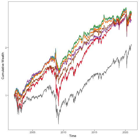
(a)

(b)

Figure 1: Cumulative wealth of benchmark portfolios EW, GMV_lin, GMV_long, GMV_nlin, GMV_robust, Index. Panel (a): 81 constituents of S&P100, time period 20020101 - 20201231 (4781 daily returns); panel (b)) 600 random constituents of Russell3000, time period 20120101 - 20201231 (2263 daily returns)

Naturally, for investors, Cumulative Wealth ($CW$) is of high interest as a measure of performance for the period considered. The gross $CW$ for portfolio benchmarks does not vary considerably, ranging from 256% for GMV_long portfolio to 273% for EW. However, the inclusion of transaction fees changes the results: the best performing EW portfolio gains 249%, followed by GMV_robust with CW 242%. The worst performing portfolio is GMV with 188% of CW. The evolvement of gross CW of all benchmark strategies for the considered period is plotted in Figure 1.

Shrinkage estimators exhibit the lowest risk, measured by SD and tests conducted point out the significance of this difference with GMV_robust. In terms of risk-adjusted performance, the winning strategies for Gross returns are shrinkage portfolios and GMV with SR 5.71% and 5.65% respectively. However, for net returns they lose half of their performance, ending up with 2.3%, whereas SR of our approach stays more stable changing from 4.26% to 3.2%. In addition, conducted tests of difference significance support the hypothesis of equal SRs, although it can be noticed that the difference is becoming more prominent for net returns.

Finally, GMV_robust dominates other benchmarks in terms of Calmar ratio. The drawdowns often determine whether a buy-side investor can keep an investment or will have to unwind and thus miss subsequent recoveries, what makes it an important risk measure for buy-side investors and managers.

Discussion of Russell3000 data set results

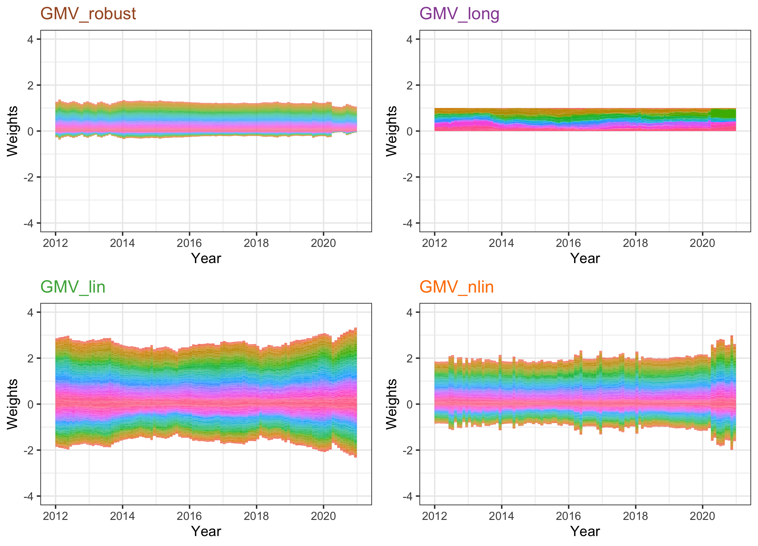
Figure 5: Weights of assets in GMV portfolios, 600 Russell3000 constituents, 20120101 - 20201231

Outcomes of weights stability analysis are consistent with ones described for S&P100 data set. GMV_robust weights are characterized by harmonized weights without extreme short or long values. It is visible in the Figure 5 and in the Table 5: GMV_robust $MAD-EW$ and $max-min$ are the lowest in comparison with benchmark portfolios (excluding EW).

In terms of accumulated wealth, GMV_robust for large portfolios performs very close to shrinkage estimators, Table 4 summarizes investment performance characteristics. Thus, GMV_robust gains in the end of the period 210 % of initial value while GMV_lin and GMV_nlin 209% and 201.9%. But considering non-zero trading fees would change the rank drastically, making the best performing benchmark Index itself, followed by GMV_robust. The findings for other risk measures stay in line with findings for S&P100:

• the less risky portfolios with the lowest SD are shrinkage portfolios, and the difference is significant in relation to GMV_robust.

• Shrinkage estimators demonstrate the highest SR for gross returns, but for the net returns GMV_robust overperforms, although difference tests do not prove the significance of the result.

• GMV_robust dominates other strategies in terms of CR for both net and gross returns.

Thus, according to outcomes of empirical experiments we can claim that GMV_robust portfolio policy achieves its goal and substantially reduces fluctuations of weights, leading to the lowest level of accumulated transaction costs. The risk adjusted performance is equal or slightly lower than shrinkage benchmarks and higher than constrained rules. Our approach is of specific interest for invetors and managers who focus on the worst drawdowm. This conclusion stays robust for small and large portfolios.

			Gross return				Net return
	TTO, %	TO, %	CW	SD, %	SR, %	CR, %	CW	SD, %	SR , %	CR, %
GMV_robust	21.59	25.45	2.72	0.94	4.26	22.22	2.42	0.94	3.19	17.44
EW	0.00	20.40	2.73	1.26	3.17	11.91	2.49	1.26	2.38	9.63
	(0.00)	(0.00)		(0.00)	(0.21)			(0.00)	(0.36)
GMV	72.89	71.37	2.70	0.86	5.65	20.32	1.88	0.86	2.33	8.37
	(0.00)	(0.00)		(0.00)	(0.75)			(0.00)	(0.26)
GMV_long	17.77	13.33	2.56	0.89	3.37	19.30	2.40	0.89	3.37	17.02
	(0.00)	(0.00)		(0.00)	(0.77)			(0.00)	(0.80)
GMV_lin	59.51	63.03	2.74	0.85	5.71	21.68	2.02	0.85	2.35	11.05
	(0.00)	(0.00)		(0.00)	(0.57)			(0.00)	(0.43)
GMV_nlin	53.33	59.10	2.69	0.85	5.71	20.69	2.01	0.85	2.35	10.82
	(0.00)	(0.00)		(0.00)	(0.66)			(0.00)	(0.40)
Index	0.00	0.00	1.91	1.22	1.82	10.82	1.91	1.22	1.82	10.82
	(0.00)	(0.00)		(0.00)	(0.01)			(0.00)	(0.08)

Table 2: Out-of-sample performance measures of benchmark portfolios, 81 stocks of S&P100, monthly rebalancing: TTO, target turnover; TO, Turnover; CW, cumulative Wealth; SD, standart deviation; SR, Sharpe ratio; CR, Calmar ratio. All estimates are obtained from daily values (4781 out-of-sample returns) for both gross and net returns. Time period: 20020101 - 20201231. The difference tests for the turnovers are obtained from a sample $t$-test. The difference test on the Sharpe ratio and Variance used the approach of Ledoit and Wolf (2008) and Ledoit and Wolf (2011), for which the R code is available at M. Wolf’s website. $p$-values are reported in parentheses with respect to the GMV_robust portfolio. RobustM_PerformanceSP100

	min	max	sd	mad-ew	max-min
GMV_robust	$-0.0268$	0.0458	0.0158	0.0127	0.0726
EW	0.0123	0.0123	0.0000	0.0000	0.0000
GMV	$-0.1167$	0.2444	0.0572	0.0405	0.3611
GMV_long	0.0000	0.2430	0.0379	0.0200	0.2430
GMV_lin	$-0.0952$	0.1951	0.0493	0.0361	0.2903
GMV_nlin	$-0.0865$	0.1787	0.0449	0.0333	0.2653

Table 3: Average characteristics of the weight vectors of GMV portfolios, 81 stocks of S&P100, monthly rebalancing. Time period: 20020101 - 20201231 RobustM_PerformanceSP100

			Gross return				Net return
	TTO, %	TO, %	CW	SD, %	SR, %	CR, %	CW	SD, %	SR , %	CR, %
GMV_robust	27.58	40.51	2.10	0.90	5.56	31.70	1.88	0.90	4.44	24.26
EW	0.00	26.81	1.92	1.23	3.25	18.73	1.78	1.24	2.42	14.56
	(0.00)	(0.00)		(0.00)	(0.10)			(0.00)	(0.29)
GMV_long	19.00	19.73	1.81	0.74	5.41	19.24	1.70	0.74	4.05	16.28
	(0.00)	(0.00)		(0.00)	(0.58)			(0.00)	(0.99)
GMV_lin	144.97	127.22	2.09	0.68	7.35	31.14	1.41	0.68	2.94	9.81
	(0.00)	(0.00)		(0.00)	(0.33)			(0.00)	(0.29)
GMV_nlin	102.25	91.75	2.02	0.65	6.15	31.44	1.53	0.65	3.08	14.56
	(0.00)	(0.00)		(0.00)	(0.34)			(0.00)	(0.65)
Index	0.00	0.00	2.10	1.06	4.57	14.56	2.10	1.06	4.57	14.56
	(0.00)	(0.00)		(0.00)	(0.51)			(0.00)	(0.76)

Table 4: Out-of-sample performance measures of benchmark portfolios, 600 stocks of Russell3000, monthly rebalancing: TTO, target turnover; TO, Turnover, TC, transaction costs; CW, cumulative Wealth; SD, standart deviation; SR, Sharpe ratio; CR, Calmar ratio. All estimates are obtained from daily values (2265 out-of-sample returns) for both gross and net returns. Time period: 20120101 - 20201231. The difference tests for turnovers are obtained from a sample $t$-test. The difference test on the Sharpe ratio and Variance used the approach of Ledoit and Wolf (2008) and Ledoit and Wolf (2011), for which the R code is available at M. Wolf’s website. $p$-values are reported in parentheses with respect to the GMV_robust portfolio. RobustM_PerformanceRussell3000

RobustM_PerformanceRussell3000

	min	max	sd	mad-ew	max-min
EW	0.0017	0.0017	0.0000	0.0000	0.0000
GMV_robust	$-0.0069$	0.0104	0.0027	0.0021	0.0174
GMV_long	0.0000	0.1383	0.0100	0.0031	0.1383
GMV_lin	$-0.0290$	0.0430	0.0095	0.0073	0.0721
GMV_nlin	$-0.0185$	0.0319	0.0067	0.0050	0.0504

Table 5: Average characteristics of the weight vectors of GMV portfolios, 600 stocks of Russell3000, monthly rebalancing. Time period: 20020101 - 20201231 RobustM_PerformanceRussell3000

7 Conclusion and discussion

“Robustifying Markowitz” has seen many attempts that are mostly based on robustifying the original simple inversion formula for exact determination of optimal GMV weights. In bypassing this “error maximizing” technique, we have presented a tool fixing the portfolio weights in a low cost re-balancing ballpark. Using modern results from robust statistics, we have constructed an algorithm that provides a computationally effective estimator for GMV Markowitz portfolios. We have shown that it suffices to utilize a PGD procedure to optimize the portfolio weights without estimating the covariance operator itself. The focus on just the PGD updates significantly distinguishes our approach from the previous techniques. We have successfully derived almost Gaussian properties of this estimator in nice ($N/T$ small) and not-so-nice ($N/T$ big) condition cases.

The weights developed with the robustified approach are less sensitive to deviations of the asset-return distribution from normality than those of the traditional minimum-variance policy. Empirical studies confirm that the proposed policies are indeed more stable and cost-reducing. The stability of the proposed portfolios makes them a feasible alternative to traditional portfolios.

The proposed toolbox improves the stability properties of weights, leading to better investment characteristics of allocation policies. Although inferior at the risk level measured by SD, our algorithm reaches a superior risk-adjusted performance (Sharpe and Calmar ratios) for net returns due to a substantial reduction of trading volume measured by turnover. Finally, these performance results are confirmed across small and large portfolios. Even for dimensions of portfolio size larger than the length of the estimation window (e.g., the Russell3000 data), the above claim pertains.

Appendix A Simulation study

In Section 4, we have shown the convergence properties of our iterative algorithm depending on the number of steps taken. Here, we use simulations to study these properties empirically. In addition, we demonstrate numerically that using a robust estimator of $\Sigma w$ improves the confidence bounds for the GMV risk.

Convergence of the algorithm

We first generate $T=250$ independent observations from Gaussian distribution. To get closer to the real distribution, we use a covariance matrix estimated from the real dataset.

We take a 250 days window from 2012-08-27 to 2013-08-26 of $N=82$ constituents of S&P100, and compute their sample covariance denoted as $S_{1}$. The corresponding optimal GMV weights $w_{1}=(S_{1}^{-1}\mathbf{1})/(\mathbf{1}^{\top}S_{1}^{-1}\mathbf{1})$ are rather explosive and have the maximal absolute weight $0.24$, which is $\approx 20$ times bigger than for the equally weighted portfolio.

It is arguable whether the true optimal portfolio weights are explosive in reality. We additionally consider a modified covariance matrix, that is obtained by rotating the eigenbasis with minimal efforts, so that the vector of ones $\mathbf{1}=(1,1,\dots,1)^{\top}$ belongs to the span of top $15$ eigenvectors. By taking $S_{2}=RS_{1}R^{\top}$, where $R$ is a rotation matrix, we ensure that $\|S_{1}-S_{2}\|/\|S_{1}\|\approx 0.13$, while $S_{2}^{-1}\mathbf{1}$ is not as explosive, and so are the optimal GMV weights $w_{2}=(S_{2}^{-1}\mathbf{1})/(\mathbf{1}^{\top}S_{2}^{-1}\mathbf{1})$. To be precise, the absolute maximal weight becomes $0.08$, which is 3x smaller than for the original sample covariance.

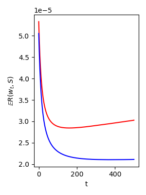
(a)

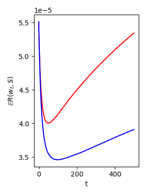
(b)

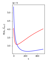
(c)

Figure 2: The graphs (a), (b) show simulated expected risk $\mathsf{E}R(w_{s},\Sigma)$ (red), expected in-sample risk $\mathsf{E}R(w_{s},\hat{\Sigma})$ (blue) for $\Sigma=S_{1}$ (a) and $\Sigma=S_{2}$ (b). The graph (c) shows in-sample risk (blue) for the S&P100 data between 2012-08-27 and 2013-08-26, and the out-of-sample risk (red) estimated using the time window between 2013-08-27 and 2014-01-17.

RobustM_Simulations

In Figures 2(a)–2(c) the blue line shows the (expected) in-sample risk of $w_{s}$, the $s$th iteration of the algorithm, depending on the number of steps. The red line shows the population or out-of-sample risk. In Figures 2(a) and 2(b), the generated data has Gaussian distribution with covariance $S_{1}$ and $S_{2}$, respectively (we take zero mean, since the estimator is translation invariant, and the risk measure does not depend on it). Notice that although the in-sample risk generally decreases with a growing number of steps, the population risk $\mathsf{E}R(w_{s},S_{j})$ has a single minimum, which confirms the tradeoff stated in Lemma 4.1, where a specific number of steps needs to be taken to achieve the bound. Using Figure 2(c) we can compare the simulated data with real, where the blue line represents one realization of the in-sample risk, using the data from 2012-08-27 to 2013-08-26, and the red line shows the out-of-sample risk that is calculated using the data from 2013-08-27 to 2014-01-17. This graph shows similar features as the first two. Notice that the curve is steeper in cases (b) and (c). Motivated by this we will use the covariance matrix $S_{2}$ for further simulations.

Heavy tailed simulation

We further investigate the effect of using a robust estimator with heavy-tailed data. In particular, we want to compare the performance of a robust estimator against the classical one. Recall, that our algorithm consists of iterative updates,

$$w_{0}=\mathbf{1}/N,\qquad w_{s}=\Pi_{1}[w_{s-1}-\eta\hat{a}(w_{s-1})],$$

where $\Pi_{1}$ is defined in (5), and $\hat{a}(w)$ is a robust estimator of $\Sigma w$. What happens if we replace it with the standard empirical version $\hat{\Sigma}w$? Below we demonstrate that using a robust estimator improves the high probability bounds.

For simulations, we construct a heavy-tailed distribution of the form $X=S_{2}^{1/2}Y$, where

$$Y\sim 0.999\times\mathcal{N}(0,\mathbf{I})+0.001\times D,$$ (13)

i.e., with probability $0.999$, $Y$ is sampled from a standard normal distribution and, with a small probability $0.001$, from a heavy-tailed distribution $D$. In our example, $D$ is supported in $\{-1,1\}^{82}$. To sample a vector $Z\sim D$, we first take a random integer $k$ uniformly in the set $\{0,1,\dots,N=82\}$. Then, we take a random subset $B$ of $\{1,\dots,82\}$ of size $k$, uniformly over all such subsets. Then, we assign $Z_{i}=1$ for $i\in B$ and $Z_{i}=-1$ otherwise. Due to the symmetry, we have $\mathsf{E}Z=0$, and it is straightforward to calculate that $\mathrm{Var}(Z)=\tfrac{2}{3}\mathbf{I}+\tfrac{1}{3}\mathbf{1}\mathbf{1}^{\top}$. Then, the covariance matrix of $X=S_{2}^{1/2}Y$ is as follows,

$$\mathrm{Var}(X)=S_{2}^{1/2}\left[\tfrac{1}{3}2.999\times\mathbf{I}+\tfrac{1}{3}0.001\times\mathbf{1}\mathbf{1}^{\top}\right]S_{2}^{1/2}\,.$$

The eigenvalues of the matrix in the middle are in the range $[0.999,1.055]$, so that $\mathrm{Var}(X)$ is only a slight perturbation of the original covariance $S_{2}$.

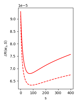
(a)

(b)

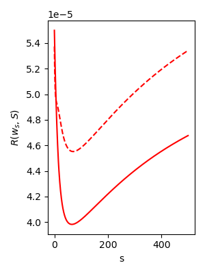
(c)

Figure 3: Graph (a) shows expected risk $\mathsf{E}R(w_{s},\Sigma)$ for the robust and non-robust (dashed) estimators. Graph (b) shows 95% quantile of the risk in the same setting. Graph (c) shows the risk of robust and non-robust estimators with one contaminated observation.

RobustM_Simulations

We generate $200$ independent samples of size $250$ from this distribution. For each sample, we compute the true risk of $s$-th iteration, given that we know exactly the covariance matrix. Figure 3(a) shows the average risk of $w_{s}$ depending on the number of iterations, and Figure 3(a) shows its $95\%$ quantile, which are calculated by taking the mean and percentile of these $200$ independent simulations, respectively. The thick line represents the risk of the robust procedure, while the dashed line corresponds to the non-robust version of the algorithm with $\hat{a}(w)$ replaced by $\hat{\Sigma}w$. It is evident, that while there is no improvement on average, the robust estimator has significantly better tails. In addition, Figure 3(c) shows what happens when we treat the heavy part of the distribution as contamination. We generate a single realization of a Gaussian sample and replace the first element with a random realization sampled from  $D$. In this case, we calculate the risk using the original covariance matrix $S_{2}$.

Appendix B Proofs

B.1 Proof of Proposition 2.1

Before we proceed, let us recall some of the results and definitions from Lugosi and Mendelson (2019b) and Hopkins et al. (2020). We start by giving the definition of a combinatorial center. It is the central object in the original construction of Lugosi and Mendelson, but the definition itself is due to Hopkins et al.

Definition B.1 (Combinatorial center).

A point $\theta\in\mathbb{R}^{N}$ is called an $(r,\kappa)$-combinatorial center of $Y_{1},\dots,Y_{\ell}$ if for all unit vectors $v\in\mathbb{R}^{N}$, the inequality

$$|v^{\top}(Y_{j}-\theta)|\leq r$$

takes place for at least $(1-\kappa)\ell$ of indices $j=1,\dots,\ell$.

Essentially, Lugosi and Mendelson (2019b) prove that for appropriately chosen $r_{\delta}$, the true mean is an $(r_{\delta},1/4)$-combinatorial center, with probability at least $1-\delta$, where $Y_{j}$ are the bucket means (see their paper for exact definitions). The estimation strategy is then executed by what is called a median-of-means tournament: one needs to pick an $(r,1/4)$-combinatorial center with $r$ as small as possible. The deviation bound then follows by a simple triangle inequality. One difficulty of implementing this strategy computationally is the lack of control on how these subsets of indices behave for different directions $v\in\mathbb{R}^{N}$.

In addition, Hopkins et al. (2020) define the spectral center as follows.

Definition B.2 (Spectral center).

For $\varepsilon\in(0,1/2)$, denote

$$\Delta_{\ell,\varepsilon}=\left\{u\in\mathbb{R}^{\ell}:\;\sum_{j=1}^{\ell}u_{j}=1,\;\;0\leq u_{j}\leq 1/\{\ell(1-\varepsilon)\}\right\}\,.$$

A point $\theta\in\mathbb{R}^{N}$ is called an $(r,\varepsilon)$-spectral center if there are weights $(u_{1},\dots,u_{\ell})\in\Delta_{\ell,\varepsilon}$ such that

$$\left\|\sum_{j=1}^{\ell}u_{j}(Y_{j}-\theta)(Y_{j}-\theta)^{\top}\right\|\leq r^{2}.$$

It is straightforward to see that if $\theta$ is a $(r,\varepsilon)$-spectral center with minimal $r$, then it has the form $\theta=\sum_{j=1}^{\ell}u_{j}Y_{j}$ for some $(u_{1},\dots,u_{\ell})\in\Delta_{\ell,\varepsilon}$, i.e., the solution should be a weighted mean of $Y_{j}$. The two definitions are “equivalent” in the following sense.

Lemma B.1.

Suppose that $\theta$ is an $(r,\kappa)$-combinatorial center. Then it is also a $(5r,10\kappa)$-spectral center. Conversely, if $\theta$ is an $(r,\varepsilon)$-spectral center, then it is also a $(\sqrt{(1-\varepsilon)/\varepsilon}\,r,2\varepsilon)$-combinatorial center.

Hopkins et al. (2020) state this lemma for some particular constants $\varepsilon$ and $\kappa$. Their proof consists of some arguments of the proof of Proposition 1 in Depersin and Lecué (2022). For the sake of completeness, we reproduce these arguments in Section B.2, slightly changed.

We deal with both notions of centers for the following reason: it is easier to deal with the statistical properties of combinatorial centers, whereas the spectral centers are more convenient from computational perspective. Hopkins, Li and Zhang (2020) develop an algorithm, namely their Algorithm $1$, that finds a spectral center with the radius that is guaranteed at most (say) twice as large as minimal possible. Namely, we denote the output of their algorithm as $\mathsf{HLZ}(Y_{1},\dots,Y_{\ell};\varepsilon)$ and they show that the output $\hat{\mu}$ satisfies

$$\min_{u\in\Delta_{\ell,\varepsilon}}\left\|\sum_{j=1}^{\ell}u_{j}(Y_{j}-\hat{\mu})(Y_{j}-\hat{\mu})^{\top}\right\|\lesssim\min_{\theta}\min_{u\in\Delta_{\ell,\varepsilon}}\left\|\sum_{j=1}^{\ell}u_{j}(Y_{j}-\theta)(Y_{j}-\theta)^{\top}\right\|\,.$$ (14)

Hence our goal is to show that with high probability, the true mean is an $(r,\varepsilon)$-spectral center with some fixed $\varepsilon$ and sufficiently small $r$, which we can do using the median-of-means analysis and switching back and forth between spectral and combinatorial centers.

Let us now give the description of the estimator $\hat{a}_{\delta}(w)$. It consists of the following steps:

1. First we centralize our observations. For this, consider the transformations $\widetilde{X}_{1}=(X_{1}-X_{2})/\sqrt{2},\widetilde{X}_{2}=(X_{3}-X_{4})/\sqrt{2},\dots$ Obviously, each of these new “observations” has zero mean and the same covariance as $X_{i}$, and moreover they are independent.

2. Fix $\varepsilon<10/21$ and set $\ell=\lceil 2(\varepsilon/10)^{-2}\log(2/\delta)\rceil$. Split the observations $\widetilde{X}_{1},\dots,\widetilde{X}_{\lfloor T/2\rfloor}$ into $\ell$ non-intersecting buckets

   $$B_{1}\sqcup\dots\sqcup B_{\ell}=\{1,\dots,\lfloor T/2\rfloor\}.$$

3. Next, using the data from each of the buckets, we construct the following covariance estimators,

   $$\Sigma_{j}=\frac{1}{|B_{j}|}\sum_{i\in B_{j}}\widetilde{X}_{i}\widetilde{X}_{i}\mathbf{1}_{\|\widetilde{X}_{i}\|\leq D}.$$

4. For a given direction $w\in\mathbb{R}^{N}$, we output the result of the $\mathsf{HLZ}$ algorithm applied to the bucket means

   $$\hat{a}_{\delta}(w)\overset{\mathrm{def}}{=}\mathsf{HLZ}(\Sigma_{1}w,\dots,\Sigma_{\ell}w;\varepsilon)\,.$$

Remark B.1.

Notice that given $\varepsilon<10/21$ and fixing, say, $\delta=0.05$, we have that the number of buckets $\ell=\lceil 2(\varepsilon/10)^{-2}\log(2/\delta)\rceil$ has to be at least $1500$, which makes the algorithm rather impractical. Unfortunately, our techniques do not allow more adequate constants. In the empirical study we heuristically choose $\varepsilon=1/3$ and $\ell=10$.

By considering $(X_{1}-X_{2})/\sqrt{2},(X_{3}-X_{4})/\sqrt{2},\dots$ we guarantee that our observations are zero mean without changing the covariance matrix. We have done so by reducing the size of the sample by at most two. To avoid the notation overloading, we assume below that $\mu=0$ and proceed to work with the original $X_{i}$.

Set $Z_{i}={X}_{i}{X}_{i}^{\top}\mathbf{1}[\|{X}_{i}\|<D]$. According to steps 2 and 3 of the algorithm, we split the data into $\ell$ blocks $B_{1},\dots,B_{\ell}$ and consider the trimmed covariances,

$${\Sigma}_{j}=\frac{1}{|B_{j}|}\sum_{i\in B_{j}}Z_{i}\,.$$

Below we derive the following bound: with probability $1-\delta$, we have that for any directions $v,w$, the inequality

$$|u^{\top}{\Sigma}_{j}w-u^{\top}\Sigma w|\lesssim\Delta_{\Sigma}\overset{\mathrm{def}}{=}\|\Sigma\|\sqrt{\frac{\mathbf{r}(\Sigma)\log\mathbf{r}(\Sigma)+\ell}{T}}$$ (15)

holds for at least $1-\kappa$ fraction of the indices $j=1,\dots,\ell$, where $\kappa=\varepsilon/10$ is fixed. Let us first complete the proof given this inequality.

At Step 5 of the algorithm, we produce the vectors $Y_{j}=\Sigma_{j}w$. On the event from (15), we have that for any unit $u\in\mathbb{R}^{N}$, the inequality

$$|u^{\top}(Y_{j}-\Sigma w)|\leq C\Delta_{\Sigma}$$

holds for at least $1-\kappa$ a fraction of indices. Hence, $\Sigma w$ is a $(C\Delta_{\Sigma},\kappa)$-combinatorial center of $Y_{j}$. By Lemma B.1, it also means that $\Sigma w$ is a $(5C\Delta_{\Sigma},10\kappa)$-spectral center of $Y_{j}$. Hence, by (14), the output of $\hat{a}_{\delta}(w)=\mathsf{HLZ}(Y_{1},\dots,Y_{j};\varepsilon)$ is a $(C^{\prime}\Delta_{\Sigma},10\kappa)$-spectral center, and using the second part of Lemma B.1, we conclude that it is also a $(C^{\prime}\sqrt{10/\kappa}\Delta_{\Sigma},20\kappa)$-combinatorial center. Since $21\kappa<1$, we get that $1-20\kappa+1-\kappa>1$, which means that for any direction $u\in\mathbb{R}^{d}$, by the pigeonhole principle, we can pick a single $Y_{j}$ that is close to both combinatorial centers $\Sigma w$ and $\hat{a}_{\delta}(w)$ in this direction. Therefore, by the triangle inequality,

$$|u^{\top}(\hat{a}_{\delta}(w)-\Sigma w)|\lesssim\Delta_{\Sigma},$$

and since the bound holds in arbitrary direction $u$, we get the required bound in Euclidean norm.

It remains to prove the bound (15). Let $\widetilde{\Sigma}=\mathsf{E}Z_{i}$. We have by Lemma 2.1 of Mendelson and Zhivotovskiy (2020),

$$\|\Sigma-\widetilde{\Sigma}\|\lesssim\frac{\|\Sigma\|^{2}\mathbf{r}(\Sigma)}{D^{2}}\,.$$ (16)

Let ${Quant}_{\alpha}(z_{1}\dots z_{\ell})$ of a sequence of real numbers denotes an order statistics $z_{(\lceil\alpha\ell\rceil)}$, where $z_{(1)}\dots z_{(k)}$ is a non-decreasing rearrangement of the original sequence. Then, we can rewrite (15) as follows,

$$\max\left\{Quant_{1-\kappa}(u^{\top}\Sigma_{j}w)-u^{\top}\Sigma w,u^{\top}\Sigma w-Quant_{\kappa}(u^{\top}\Sigma_{j}w)\right\}\lesssim\Delta_{\Sigma}\,.$$

Let us apply Klochkov et al. (2021, Lemma 2.3) to the class of functions $\{f_{u,w}(Y)=u^{\top}Yw\}$. We have that with probability at least $1-2e^{-\kappa^{2}\ell/2}$,

$$\max\left\{Quant_{1-\kappa}(u^{\top}\Sigma_{j}w)-u^{\top}\Sigma w,u^{\top}\Sigma w-Quant_{\kappa}(u^{\top}\Sigma_{j}w)\right\}\\ \lesssim\mathsf{E}\sup_{u,w}\left(\frac{1}{T}\sum_{i=1}^{N}\varepsilon_{i}u^{\top}Y_{i}w\right)+\sqrt{\sup_{u,w}\mathsf{E}(u^{\top}Y_{1}w)^{2}\frac{\ell}{T}}+\|\widetilde{\Sigma}-\Sigma\|\,,$$

where $\varepsilon_{1},\dots,\varepsilon_{n}$ are independent Rademacher signs, i.e., taking $\pm 1$ with probability $1/2$. The supremum in both terms of the RHS is over unit vectors $u,w$ in $\mathbb{R}^{N}$. Let us first bound the second, weak term. We have that

$$\mathsf{E}(u^{\top}Y_{1}w)^{2}\leq\mathsf{E}(u^{\top}X_{1})^{2}(w^{\top}X_{1})^{2}\leq\mathsf{E}^{1/2}(u^{\top}X_{1})^{4}\mathsf{E}^{1/2}(w^{\top}X_{1})^{4}\,.$$

By the $L_{4}$–$L_{2}$ equivalence assumption we get that $\mathsf{E}^{1/2}(u^{\top}X_{1})^{4}\lesssim\mathsf{E}(u^{\top}X_{1})^{2}\leq\|\Sigma\|$. The weak term is therefore bounded by $C\|\Sigma\|\sqrt{\ell/T}$.

Now let us deal with the first, strong term. We rewrite it as follows,

$$\mathsf{E}\sup_{u,w}\left(\frac{1}{T}\sum_{i=1}^{N}\varepsilon_{i}u^{\top}Y_{i}w\right)=\mathsf{E}\sup_{u,w}u^{\top}\left(\frac{1}{T}\sum_{i=1}^{N}\varepsilon_{i}Y_{i}\right)w=\mathsf{E}\left\|\frac{1}{T}\sum_{i=1}^{N}\varepsilon_{i}Y_{i}\right\|.$$

The right-most expression is the expected value of the norm of a sum of centered matrices $\varepsilon_{i}Y_{i}$, which are bounded by $D^{2}$ pointwise. We therefore can apply the Matrix Bernstein inequality, the details are carried out by Mendelson and Zhivotovskiy (2020). They show that this leads eventually to the bound

$$\mathsf{E}\left\|\frac{1}{T}\sum_{i=1}^{T}\varepsilon_{i}Y_{i}\right\|\lesssim\|\Sigma\|\sqrt{\frac{\mathbf{r}(\Sigma)\log\mathbf{r}(\Sigma)}{T}}+\frac{D^{2}\log\mathbf{r}(\Sigma)}{T}\,.$$

Recalling the bound (16) we get that, with probability $1-2e^{-\kappa^{2}\ell/2}$,

$$\max\left\{Quant_{1-\kappa}(u^{\top}\Sigma_{j}w)-u^{\top}\Sigma w,u^{\top}\Sigma w-Quant_{\kappa}(u^{\top}\Sigma_{j}w)\right\}\\ \lesssim\Delta_{\Sigma}+\frac{D^{2}\log\mathbf{r}(\Sigma)}{T}+\frac{\|\Sigma\|^{2}\mathbf{r}(\Sigma)}{D^{2}}\,.$$

For $D\sim\|\Sigma\|^{1/2}\left(\frac{T\mathbf{r}(\Sigma)}{\log\mathbf{r}(\Sigma)}\right)^{1/4}$ the RHS simplifies to $\Delta_{\Sigma}=\|\Sigma\|\sqrt{\frac{\mathbf{r}(\Sigma)\log\mathbf{r}(\Sigma)+\ell}{T}}$. It remains to notice that $1-2e^{-\kappa^{2}\ell/2}\geq 1-\delta$ as long as $\ell\geq 2\kappa^{-2}\log\left(\frac{2}{\delta}\right)$.

B.2 Proof of Lemma B.1

Let us first recall the following basic fact from linear algebra: for a symmetric matrix $A$, its largest eigenvalue satisfies $\lambda_{\max}(A)=\sup_{M\succeq 0,\operatorname{Tr}(M)=1}\operatorname{Tr}(MA)$. Hence, we can rewrite

$$\min_{w\in\Delta_{\ell,\varepsilon}}\left\|\sum_{j=1}^{\ell}w_{j}(Y_{j}-\theta)(Y_{j}-\theta)^{\top}\right\|=\min_{w\in\Delta_{\ell,\varepsilon}}\max_{M\succeq 0,\operatorname{Tr}(M)=1}\sum_{j=1}^{\ell}w_{j}(Y_{j}-\theta)^{\top}M(Y_{j}-\theta).$$

The latter can be seen as semi-definite program (SDP) and using the strong duality of SDP one can show that the minimum over $w$ and the maximum over $M$ can be swapped (see formula (5.2) in Hopkins et al. (2020); see also Depersin and Lecué (2022); Diakonikolas et al. (2020)):

$$\min_{w\in\Delta_{\ell,\varepsilon}}\max_{M\succeq 0,\operatorname{Tr}(M)=1}\sum_{j=1}^{\ell}w_{j}(Y_{j}-\theta)^{\top}M(Y_{j}-\theta)$$

$$=\max_{M\succeq 0,\operatorname{Tr}(M)=1}\min_{w\in\Delta_{\ell,\varepsilon}}\sum_{j=1}^{\ell}w_{j}(Y_{j}-\theta)^{\top}M(Y_{j}-\theta).$$

The right-hand side form is closer to what Lugosi and Mendelson (2019b) do: for any direction $M=vv^{\top}$ we can pick its own weights. This property allows to show the equivalence.

We write $y_{j}=Y_{j}-\theta$ for short everywhere in this section. First, assume that $\theta$ is a $(r,\kappa)$-combinatorial center. We will show by contradiction that it is also a $(\tilde{r},\varepsilon)$-spectral center, where $\tilde{r}=5r$ and $\varepsilon=10\kappa$. Suppose it is not, so that for some $M\succeq 0$ with $\operatorname{Tr}(M)=1$ we have that

$$\min_{w\in\Delta_{\ell,\varepsilon}}\sum_{j}w_{j}y_{j}^{\top}My_{j}\geq\tilde{r}^{2}\,.$$

If $w\in\Delta_{\ell,\varepsilon}$ delivers the minimum it must put non-zero weights to at least $\lceil\ell(1-\varepsilon)\rceil$ terms. Since the weights sum up to one, we conclude that for at least $\lceil\ell\varepsilon\rceil$ indices $j=1,\dots,\ell$, it holds that $y_{j}^{\top}My_{j}\geq\tilde{r}^{2}$. We denote this set of indices as $B$. Now, let $M=\sum_{k=1}^{\ell}\lambda_{k}u_{k}u_{k}^{\top}$ be its spectral decomposition. Since $M\succeq 0$ and $\operatorname{Tr}(M)=1$, we have that $\sum_{k}\lambda_{k}=1$ and $\lambda_{k}\geq 0$.

Let us take a random unit vector $v=\sum_{k}\sqrt{\lambda_{k}}u_{k}\varepsilon_{k}$, where $\varepsilon_{k}$ are independent random signs, so that the equality $\sum_{k}\lambda_{k}=1$ ensures that it is indeed a unit vector. Moreover,

$$y_{j}^{\top}v=\sum_{k}(\sqrt{\lambda_{k}}y_{j}^{\top}u_{k})\varepsilon_{k}=\sum_{k}a_{k}^{(j)}\varepsilon_{k},$$

where we denote $a_{k}^{(j)}=\sqrt{\lambda_{k}}y_{j}^{\top}u_{k}$, and we also denote by $a^{(j)}\in\mathbb{R}^{\ell}$ the vector with corresponding coordinates. Observe that for $j\in B$, we have that

$$\|a^{(j)}\|^{2}=\sum_{k}\lambda_{k}y_{j}^{\top}u_{k}u_{k}^{\top}y_{j}=y_{j}^{\top}My_{j}\geq\tilde{r}^{2}.$$

The Khintchin inequality due to Szarek (1976) states that,

$$\frac{1}{\sqrt{2}}\|a^{(j)}\|\leq\mathsf{E}\left|\sum_{k}a_{k}^{(j)}\varepsilon_{j}\right|\leq\|a^{(j)}\|\,.$$

Furthermore, the lower tail of the bounded differences inequality (Theorem 6.9 in Boucheron et al. (2013)) implies that

$$\mathsf{P}\left(\left|\sum_{k}a_{k}^{(j)}\varepsilon_{j}\right|<\frac{1}{\sqrt{2}}\|a^{(j)}\|-t\right)\leq e^{-\frac{t^{2}}{2(\|a^{(j)}\|^{2}+t\|a^{(j)}\|/3)}}.$$

Taking $t=\frac{1-c}{\sqrt{2}}\|a^{(j)}\|$, we get that

$$\mathsf{P}\left(\left|\sum_{k}a_{k}^{(j)}\varepsilon_{j}\right|\geq\frac{c}{\sqrt{2}}\|a^{(j)}\|\right)\geq 1-e^{-\frac{(1-c)^{2}}{4(1+(1-c)/(3\sqrt{2}))}},$$

which for $c=\sqrt{2}/5$ is greater than $0.1$. Hence, we can find a unit vector $v$ such that for at least one tenth of the indices $j\in B$,

$$|y_{j}^{\top}v|\geq\frac{1}{5}\tilde{r}=r.$$

One tenth of $B$ accounts for $0.1\varepsilon=\kappa$, hence $\theta$ cannot be an $(r,\kappa)$-combinatorial center.

Suppose that $\theta$ is a $(r,\varepsilon)$-spectral center. Again we will prove that it is also a $(\tilde{r},\kappa)$-combinatorial center by contradiction, with $\tilde{r}=\sqrt{(1-\varepsilon)/\varepsilon}\,r$, $\kappa=2\varepsilon$. Suppose it is not. Then, there is a unit vector $v$, such that for strictly more than $\ell\kappa$ indices $j$, $|y_{j}^{\top}v|>\tilde{r}$. Denote this set of indices as $B$. Since $\theta$ is a spectral center, we get that for $M=vv^{\top}$,

$$\min_{w\in\Delta_{\ell,\varepsilon}}\sum_{j=1}^{\ell}w_{j}|y_{j}^{\top}v|^{2}\leq r^{2}.$$

The minimum puts the weight $1/(\ell(1-\varepsilon))$ for $\lfloor\ell(1-\varepsilon)\rfloor$ indices $j$ with the smallest values $|y_{j}^{\top}v|$. By the pigeonhole principle, strictly more than $\ell\kappa-\lceil\ell\varepsilon\rceil$ of them are in the set $B$. Hence,

$$\min_{w\in\Delta_{\ell,\varepsilon}}\sum_{j=1}^{\ell}w_{j}|y_{j}^{\top}v|^{2}>\frac{\kappa-\varepsilon}{1-\varepsilon}\tilde{r}^{2}=\frac{\varepsilon}{1-\varepsilon}\tilde{r}^{2}=r^{2}.$$

This completes the proof by contradiction.

Appendix C Proof of Lemma 3.1

Let us first calculate $w^{*}$ explicitly. Since $-M_{\lambda}(w;\Sigma,\mu)$ is strongly convex, and adding a Lagrangian multiplier $-l(w^{\top}\mathbf{1}-1)$ corresponding to the restriction $w^{\top}\mathbf{1}=1$, we have that $w^{*}$ is the solution to

$$-\mu+\gamma\Sigma w-l\mathbf{1}=0\qquad\Rightarrow\qquad w=\frac{1}{\gamma}\Sigma^{-1}(\mu+l\mathbf{1})\,.$$

Since $w^{\top}\mathbf{1}=1$ we find that $l=(\gamma-\mathbf{1}^{\top}\Sigma^{-1}\mu)/(\mathbf{1}^{\top}\Sigma^{-1}\mathbf{1})$. Therefore,

$$w^{*}=\gamma^{-1}\Sigma^{-1}\mu+\frac{1-\gamma^{-1}\mathbf{1}^{\top}\Sigma^{-1}\mu}{\mathbf{1}^{\top}\Sigma^{-1}\mathbf{1}}\Sigma^{-1}\mathbf{1}\,.$$

Denote $\Pi_{0}=I-N^{-1}\mathbf{1}\mathbf{1}^{\top}$ the orthogonal projector onto the subspace of $\{w:\;w^{\top}\mathbf{1}=0\}$, so that $\Pi_{1}(x+y)=\Pi_{1}x+\Pi_{0}y$. It is straightforward to check that $\Pi_{0}(\gamma\Sigma w^{*}-\mu)$ vanishes, which is all we need to know about $w^{*}$ for the remaining of the proof.

Write $\Delta(w)=\gamma{(}\Sigma w-\hat{a}(w){)}-(\mu-\hat{\mu})$. Then,

$$w_{s+1}-w^{*} =w_{s}-w^{*}-\eta\Pi_{0}[\gamma\Sigma w_{s}-\mu]+\eta\Pi_{0}\Delta(w_{s})$$

$$=\left({I}-\eta\gamma\Pi_{0}\Sigma\right)(w_{s}-w^{*})+\eta\Pi_{0}\Delta(w_{s})$$

$$=\Pi_{0}({I}-\eta\gamma\Sigma)(w_{s}-w^{*})+\eta\Pi_{0}\Delta(w_{s})\,,$$

where since $\eta\leq 1/(\gamma\lambda_{\max})$, we have that ${I}-\eta\gamma\Sigma$ is positive definite, and $\|{I}-\eta\gamma\Sigma\|=1-\eta\gamma\lambda_{\min}$. In addition, due to the requirement of the theorem for the estimators $\hat{\mu}$ and $\hat{a}(w)$, we have that

$$\|\Delta(w)\|\leq\Delta_{\mu}+\gamma\Delta_{\Sigma}\|w\|\,.$$

Denoting $\delta_{s}=\|w_{s}-w^{*}\|$, we have the recursive inequality,

$$\delta_{s+1}\leq(1-\eta\gamma\lambda_{\min})\delta_{s}+\eta\Delta_{\mu}+\eta\gamma\Delta_{\Sigma}\|w_{s}\|\,.$$

We can link $\|w_{s}\|$ to $\delta_{s}$ through a simple triangle inequality $\|w_{s}\|\leq\|w^{*}\|+\delta_{s}$. We obtain,

$$\delta_{s+1}\leq{\color[rgb]{1,0,1}(}1-\eta\gamma(\lambda_{\min}-\Delta_{\Sigma}){\color[rgb]{1,0,1})}\delta_{s}+\eta\Delta_{\mu}+\eta\gamma\Delta_{\Sigma}\|w^{*}\|\,.$$

Denoting $\kappa=1-\eta\gamma(\lambda_{\min}-\Delta_{\Sigma})<1$ and $x=\eta\Delta_{\mu}+\eta\gamma\Delta_{\Sigma}\|w^{*}\|$, we expand our recursive inequality as follows,

$$\delta_{s+1} \leq\kappa\delta_{s}+x\leq\kappa^{2}\delta_{s-1}+\kappa x+x\leq\kappa^{s+1}\delta_{0}+(\kappa^{s}+\dots+1)x$$

$$<\kappa^{s+1}\delta_{0}+\frac{x}{1-\kappa}\,.$$

Substituting $\kappa$ and $x$ back, we obtain the result.

C.1 Proof of Theorem 3.1

Simply substitute $\Delta_{\mu}=C\|\Sigma\|^{1/2}\sqrt{\frac{\mathbf{r}(\Sigma)+\log(1/\delta)}{T}}$ and $\Delta_{\Sigma}=C\|\Sigma\|\sqrt{\frac{\mathbf{r}(\Sigma)\log\mathbf{r}(\Sigma)+\log(1/\delta)}{T}}$ into Lemma 3.1, and take $\eta=1/(\gamma\lambda_{\max})$. Here $C>0$ is an appropriately chosen absolute constant. The condition (10) ensures that $\Delta_{\Sigma}\leq\lambda_{\min}/2$. We get that

$$\|w_{s}-w^{*}\|\leq\left(1-\frac{1}{2\kappa}\right)^{s}\|w_{0}-w^{*}\|+C^{\prime}\frac{{\gamma^{-1}}\|\Sigma\|^{1/2}+\|\Sigma\|\|w^{*}\|}{\lambda_{\min}}\sqrt{\frac{\mathbf{r}(\Sigma)\log\mathbf{r}(\Sigma)+\log(1/\delta)}{T}}.$$

Taking $s\sim\log T$ steps, the first term will be dominated by second one. Furthermore, since the objective is quadratic and $w^{*}$ is its optimum, we have that

$$M_{\gamma}(w^{*};\Sigma,\mu)-M_{\gamma}(w_{s};\Sigma,\mu) =\frac{\gamma}{2}\|\Sigma^{1/2}(w_{s}-w^{*})\|^{2}$$

$$\lesssim\frac{{\gamma^{-1}}\|\Sigma\|^{2}+{\gamma}\|\Sigma\|^{3}\|w^{*}\|^{2}}{\lambda_{\min}^{2}}\cdot\frac{\mathbf{r}(\Sigma)\log\mathbf{r}(\Sigma)+\log(1/\delta)}{T},$$

hence the bound follows.

Appendix D Proof of Lemma 4.1

When $\Sigma$ is invertible, it is well known that the true minimum of the risk is $w^{*}=\Sigma^{-1}\mathbf{1}/(\mathbf{1}^{\top}\Sigma^{-1}\mathbf{1})$, so that $\Pi_{0}\Sigma w^{*}$ vanishes. When $\Sigma$ is not invertible, it is straightforward to check that $\Pi_{0}\Sigma w^{*}=0$ for any $w^{*}\in\mathrm{Argmin}_{w^{\top}1=1}R(w;\Sigma)$. Below we assume that $w^{*}$ is some fixed optimal solution.

Write $\Delta(w)=\Pi_{0}[\hat{a}(w)-\Sigma w]$, so that the updates take the form $w_{s+1}=w_{s}-\eta\Pi_{0}\Sigma w_{s}-\eta\Delta(w_{s})$. We first show that,

$$\|w_{s+1}-w^{*}+\eta\Delta(w_{s})\|\leq\|w_{s}-w^{*}\|\,.$$ (17)

Using $\Pi_{0}\Sigma w^{*}=0$, we have

$$w_{s+1}-w^{*}+\eta\Delta(w_{s}) =w_{s}-w^{*}-\eta\Pi_{0}\Sigma w_{s}$$

$$=w_{s}-w^{*}+\eta\Pi_{0}\Sigma w^{*}-\eta\Pi_{0}\Sigma w_{s}$$

$$=(I-\eta\Pi_{0}\Sigma\Pi_{0})(w_{s}-w^{*}),$$

where for the last line we used the fact that $(w_{s}-w^{*})=\Pi_{0}(w_{s}-w^{*})$, since both $w^{*}$ and $w_{s}$ sum up to one. Using the condition $\eta\leq 1/\|\Sigma\|$, the matrix $I-\eta\Pi_{0}\Sigma\Pi_{0}$ is a contraction, so the inequality (17) follows.

Applying further the triangle inequality, we have that

$$\|w_{s+1}-w^{*}\| \leq\|w_{s}-w^{*}\|+\|\Delta(w_{s})\|\leq(1+\eta\Delta_{\Sigma})\|w_{s}-w^{*}\|+\eta\Delta_{\Sigma}\|w^{*}\|$$

$$\leq\dots$$

$$\leq(1+\eta\Delta_{\Sigma})^{s+1}\left(\|w_{0}-w^{*}\|+s\eta\Delta_{\Sigma}\|w^{*}\|\right).$$

Let $n$ be an integer and assume that $n\eta\Delta_{\Sigma}\leq 1$. Then, using the inequality $(1+1/n)^{n}\leq e$, for each $s=0,1,\dots,n$, we have

$$\max(\|w_{s}\|,\|w_{s}-w^{*}\|)\leq(e+1)\left(\|w_{0}-w^{*}\|+\|w^{*}\|\right)\overset{\mathrm{def}}{=}M\,.$$ (18)

Further, we apply a standard trick in optimization; see e.g., Theorem 3.5 in Bubeck (2015). Let us denote $R^{*}(w)=R(w;\Sigma)$, which is a convex and $\|\Sigma\|$-smooth function. Therefore, it holds that for any $u,w$,

$$0\leq R^{*}(u)-R^{*}(w)-\nabla R^{*}(w)(u-w)\leq\frac{\|\Sigma\|}{2}\|u-w\|^{2}\,.$$ (19)

Applying this inequality for $w_{s}$ and $w_{s+1}=w_{s}-\eta\Pi_{0}\Sigma w_{s}-\eta\Delta(w_{s})$, we first obtain that

$$R^{*}(w_{s+1})-R^{*}(w_{s})\leq -\eta(\Sigma w_{s})^{\top}\left[\Pi_{0}\Sigma w_{s}+\Delta(w_{s})\right]+\frac{\eta^{2}\|\Sigma\|}{2}\left\|\Pi_{0}\Sigma w_{s}+\Delta(w_{s})\right\|^{2}$$

$$\leq -\eta(\Sigma w_{s})^{\top}\left[\Pi_{0}\Sigma w_{s}+\Delta(w_{s})\right]+\frac{\eta}{2}\left\|\Pi_{0}\Sigma w_{s}+\Delta(w_{s})\right\|^{2}$$

$$= -\frac{\eta}{2}\|\Pi_{0}\Sigma w_{s}\|^{2}+\frac{\eta}{2}\|\Delta(w_{s})\|^{2}.$$

Observe that due to (19),

$$R^{*}(w_{s})-R^{*}(w^{*})\leq(\Sigma w_{s})^{\top}(w_{s}-w^{*})\leq\|\Pi_{0}\Sigma w_{s}\|\|w_{s}-w^{*}\|\leq M\|\Pi_{0}\Sigma w_{s}\|,$$

where in the last inequality we also use the bound (18). Furthermore, $\|\Delta(w_{s})\|\leq\Delta_{\Sigma}M$. Denoting $\delta_{s}=R^{*}(w_{s})-R^{*}(w^{*})$, we obtain the recursive inequality,

$$\delta_{s+1}\leq\delta_{s}-\frac{\eta}{4M^{2}}\delta_{s}^{2}+\eta\Delta_{\Sigma}^{2}M^{2}\,.$$

Denoting additionally $\alpha_{s}=\max\{0,\delta_{s}-s\eta\Delta_{\Sigma}^{2}M^{2}\}$, we can easily derive that $\alpha_{s+1}\leq\max\left\{0,\alpha_{s}-\frac{\eta}{4M^{2}}\alpha_{s}\right\}$. It is straightforward to check that $\alpha_{0}\leq\|\Sigma\|M^{2}\leq\frac{4M^{2}}{\eta}$ and $\alpha_{s+1}\leq\alpha_{s}$. Therefore, we conclude that we can drop the positive part, so that $\frac{1}{\alpha_{s}}\leq\frac{1}{\alpha_{s+1}}-\frac{\eta}{4M^{2}}\frac{\alpha_{s}}{\alpha_{s+1}}\leq\frac{1}{\alpha_{t+1}}-\frac{\eta}{4M^{2}}$. Hence, the bound $\frac{1}{\alpha_{t}}\geq\frac{\eta}{4M^{2}}t$ follows . Therefore, the following inequality holds

$$R^{*}(w_{t})-R^{*}(w^{*})=\delta_{t}\leq\alpha_{t}+t\eta\Delta_{\Sigma}^{2}M^{2}\leq\frac{4M^{2}}{\eta t}+t\eta\Delta_{\Sigma}^{2}M^{2}\,,$$

which completes the proof.

Appendix E Weights visualization

Figure 4: Weights of assets in GMV portfolios, 81 S&P100 constituents, 20020101 - 20201231

RobustM_PerformanceSP100

RobustM_PerformanceRussell3000

Appendix F Performance results with window length $T=252$

			Gross return				Net return
	TTO , %	TO , %	CW	SD , %	SR , %	CR , %	CW	SD , %	SR, %	CR, %
GMV_robust	35.83	27.58	2.73	0.92	3.26	22.21	2.41	0.92	3.26	17.14
EW	0.00	21.24	2.66	1.27	2.36	10.79	2.44	1.27	2.36	8.45
	(0.00)	(0.00)		(0.00)	(0.19)			(0.00)	(0.34)
GMV	157.48	94.77	3.01	0.91	4.40	22.79	1.90	0.91	2.20	7.10
	(0.00)	(0.00)		(0.41)	(0.50)			(0.43)	(0.31)
GMV_long	30.43	13.92	2.67	0.86	3.49	21.61	2.52	0.86	3.49	18.72
	(0.00)	(0.00)		(0.00)	(0.80)			(0.00)	(0.41)
GMV_lin	101.49	69.98	2.97	0.84	4.76	26.47	2.15	0.84	2.38	12.21
	(0.00)	(0.00)		(0.00)	(0.26)			(0.00)	(0.70)
GMV_nlin	82.04	61.89	2.90	0.83	4.82	24.93	2.18	0.83	2.41	12.43
	(0.00)	(0.00)		(0.00)	(0.30)			(0.00)	(0.77)
Index	0.00	0.00	1.91	1.24	1.52	12.43	1.92	1.24	1.52	12.43
	(0.00)	(0.00)		(0.00)	(0.01)			(0.00)	(0.06)

Table 6: Out-of-sample performance measures of benchmark portfolios, 81 stocks of S&P100, monthly rebalancing: TTO, target turnover; TO, Turnover; CW, cumulative Wealth; SD, standard deviation; SR, Sharpe ratio; CR, Calmar ratio. All estimates are obtained from daily values (5031 out-of-sample returns) for both gross and net returns. Time period: 20010101 - 20201231.The difference tests for the turnovers are obtained from a sample $t$-test. The difference test on the Sharpe ratio and Variance used the approach of Ledoit and Wolf (2008) and Ledoit and Wolf (2011), for which the R code is available at M. Wolf’s website. $p$-values are reported in parentheses with respect to the GMV_robust portfolio. RobustM_PerformanceSP100

			Gross return				Net return
	TTO, %	TO, %	CW	SD , %	SR , %	CR , %	CW	SD , %	SR , %	CR , %
GMV_robust	40.08	41.85	2.16	0.87	5.75	29.31	1.91	0.87	4.60	21.94
EW	0.00	27.07	1.84	1.30	2.31	14.15	1.68	1.30	2.31	10.15
	(0.00)	(0.00)		(0.00)	(0.02)			(0.00)	(0.06)
GMV_long	32.24	18.12	1.67	0.84	3.57	11.11	1.56	0.84	2.38	8.97
	(0.00)	(0.00)		(0.83)	(0.12)			(0.83)	(0.29)
GMV_lin	138.52	105.99	2.14	0.66	7.58	30.61	1.51	0.66	3.03	12.02
	(0.00)	(0.00)		(0.00)	(0.26)			(0.00)	(0.42)
GMV_nlin	80.14	81.86	2.17	0.65	7.69	32.46	1.68	0.65	4.62	17.51
	(0.00)	(0.00)		(0.00)	(0.17)			(0.00)	(0.98)
Index	0.00	0.00	2.08	1.12	3.84	17.51	2.08	1.12	3.84	17.51
	(0.00)	(0.00)		(0.00)	(0.22)			(0.00)	(0.77)

Table 7: Out-of-sample performance measures of benchmark portfolios, 600 stocks of Russell3000, monthly rebalancing and : TTO, target turnover; TO, Turnover, TC, transaction costs; CW, cumulative Wealth; SD, standard deviation; SR, Sharpe ratio; CR, Calmar ratio. All estimates are obtained from daily values (2515 out-of-sample returns) for both gross and net returns. Time period: 20110101 - 20201231. The difference tests for turnovers are obtained from a sample $t$-test. The difference test on the Sharpe ratio and Variance used the approach of Ledoit and Wolf (2008) and Ledoit and Wolf (2011), for which the R code is available at M. Wolf’s website. $p$-values are reported in parentheses with respect to the GMV_robust portfolio. RobustM_PerformanceRussell3000

References

- (1)
- Abdalla and Zhivotovskiy (2022) Abdalla, P. and Zhivotovskiy, N. (2022). Covariance estimation: Optimal dimension-free guarantees for adversarial corruption and heavy tails, arXiv preprint arXiv:2205.08494 .
- Ao et al. (2019) Ao, M., Yingying, L. and Zheng, X. (2019). Approaching mean-variance efficiency for large portfolios, The Review of Financial Studies 32(7): 2890–2919.
- Bai and Li (2012) Bai, J. and Li, K. (2012). Statistical analysis of factor models of high dimension, Annals of Statistics 40(1): 436–465.
- Bai et al. (2009) Bai, Z., Liu, H. and Wong, W.-K. (2009). Enhancement of the applicability of Markowitz’s portfolio optimization by utilizing random matrix theory, Mathematical Finance 19: 639 – 667.
- Bartl and Mendelson (2022) Bartl, D. and Mendelson, S. (2022). On Monte-Carlo methods in convex stochastic optimization, Annals of Applied Probability 32(4): 3146 – 3198.
- Best and Grauer (1991) Best, M. and Grauer, R. (1991). On the sensitivity of mean-variance-efficient portfolios to changes in asset means: Some analytical and computational results, Review of Financial Studies 4: 315–42.
- Boucheron et al. (2013) Boucheron, S., Lugosi, G. and Massart, P. (2013). Concentration Inequalities: A Nonasymptotic Theory of Independence, Oxford University Press.
- Broadie (1993) Broadie, M. (1993). Computing efficient frontiers using estimated parameters, Annals of Operations Research 45(1): 21–58.
- Bubeck (2015) Bubeck, S. (2015). Convex optimization: Algorithms and complexity, Foundations and Trends in Machine Learning 8(3–4): 231–357.
- Chen and Yuan (2016) Chen, J. and Yuan, M. (2016). Efficient Portfolio Selection in a Large Market, Journal of Financial Econometrics 14(3): 496–524.
- Cherapanamjeri et al. (2019) Cherapanamjeri, Y., Flammarion, N. and Bartlett, P. L. (2019). Fast mean estimation with sub-Gaussian rates, Conference on Learning Theory, pp. 786–806.
- Cherapanamjeri et al. (2020) Cherapanamjeri, Y., Hopkins, S. B., Kathuria, T., Raghavendra, P. and Tripuraneni, N. (2020). Algorithms for heavy-tailed statistics: Regression, covariance estimation, and beyond, Proceedings of the 52nd Annual ACM SIGACT Symposium on Theory of Computing, pp. 601–609.
- Chopra and Ziemba (1993) Chopra, V. K. and Ziemba, W. T. (1993). The effect of errors in means, variances, and covariances on optimal portfolio choice, Journal of Portfolio Management 19(2): 6–11.
- DeMiguel et al. (2009) DeMiguel, V., Garlappi, L. and Uppal, R. (2009). Optimal versus naive diversification: How inefficient is the portfolio strategy?, The review of Financial Studies 22(5): 1915–1953.