Floquet topological phases on a honeycomb lattice using elliptically polarized light

Abstract

We study the effect of driving a two-dimensional honeycomb system out of equilibrium using an elliptically polarized light as a time-dependent perturbation. In particular, we try to understand the topological phase diagram of this driven system when the external drive is a vector potential given by ${\bf A}(t)=(A_{0x}\cos(\Omega t),A_{0y}\cos(\Omega t+\phi_{0}))$. These topological phases are characterized by the Floquet Chern number which, in each of these phases, is related to the number of robust edge modes on a nanoribbon. We show that varying the ratio $A_{0x}/A_{0y}$ of the external drive is a possible way to take the system from a trivial to a topological phase and vice versa.

I Introduction

One of the most promising playgrounds for both experimental and theoretical studies of topological phases in two-dimensional systems is the wonder material graphene and other related materials with similar honeycomb lattice structure. While pristine graphene is a gapless and trivial system, taking into account the effects of spin-orbit coupling (SOC) in graphene, can generate topologically non-trivial phases. Experimentally, such an SOC can be induced by proximity to a topological insulator (TI) such as bismuth selenide [1, 2] or by functionalizing graphene using methyl [3]. As in all topological systems [4, 5, 6, 7, 8], such phases are characterized by and insulating bulk, hosting conducting boundary modes. A topological invariant (for instance, a Chern number in the case of two-dimensional TIs) is derived from the bulk bands, and defines the properties of the boundary modes via the bulk boundary correspondence.

While the physics of topological phases and edge states in graphene is by itself quite intriguing to the generation of such phases by driving the system out of equilibrium [9, 10, 11, 12, 13, 14, 15, 16, 17, 18, 19, 20, 21, 22, 23, 24, 25, 26, 27, 28] is a rapidly developing field of research. Using an external perturbation periodic in time - either by varying a parameter periodically with time or by using polarized light - it is possible to modify the behavior of the system and change its topological character. In particular, we can generate topological phases by applying a time-periodic drive to a system which was non-topological to begin with. Equally interesting is the possibility of manipulating or destroying the topologically non-trivial nature of a system by using an external drive with appropriate parameters. Since we assume that these out-of-equilibrium systems are perfectly periodic in nature, we employ Floquet theory [29] to study their behavior.

There are several studies that use circularly polarized light [30] to generate and/or modify Floquet topological phases. However the more general case of elliptical polarization remains largely unexplored to the best of our knowledge. Even though the result of using an elliptically polarized light [31, 32, 33, 34, 19, 35] might appear qualitatively somewhat similar to the effect of using circular polarized light, there are some major differences. The main reason for these differences is the anisotropy which the elliptical polarization introduces into the system.

The plan of this paper is as follows. We begin in Sec. II with an overview of the spectrum and edge modes of a honeycomb lattice in presence of a staggered potential. This is followed in Sec. III by a brief description of elliptically-polarized light which is then used in Sec. IV to drive the honeycomb lattice . We find that Floquet topological phases depend not only on the frequency and amplitude of the drive but also on the relative phase between the components of the field. These phases are identified using the Chern number which is calculated using the Floquet eigenstates. Finally, in Sec, V we demonstrate the bulk boundary correspondence for these phases by studying the Floquet edge modes that lie on the boundary of a nanoribbon fashioned out of a honeycomb lattice system. The number of these edge states is found to be consistent with the Chern number of the bulk system.

II Pristine graphene at equilibrium

Spinless electrons on a honeycomb lattice are governed by the two-band momentum-space tight-binding hamiltonian

$$H=\sum_{{\bf k}}\begin{pmatrix}a_{{\bf k}}^{\dagger}&b_{{\bf k},\downarrow}^{\dagger}\end{pmatrix}h({\bf k})\begin{pmatrix}a_{{\bf k}}\\ ~{}\\ b_{{\bf k}}\end{pmatrix},$$ (1)

where $a_{\bf k}$ and $b_{\bf k}$ denote the annihilation operators for $A$ and $B$ sublattice respectively and,

$$h({\bf k})=\begin{pmatrix}+\mu_{S}&~{}&f({\bf k})\\ \\ f^{*}({\bf k})&~{}&-\mu_{S}\end{pmatrix}.$$ (2)

The off-diagonal terms denote nearest neighbor hoppings with strength $\gamma$,

$$f({\bf k})=\gamma\Big{(}1+e^{i{\bf k}\cdot\bf{v_{2}}}+e^{i{\bf k}\cdot\bf{(v_{2}-v_{1})}}\Big{)}=\gamma\Big{(}1+2\cos\frac{\sqrt{3}k_{x}}{2}e^{3ik_{y}/2}\Big{)}.$$ (3)

The vectors ${\bf v_{1}}$ and ${\bf v_{2}}$ are the spanning vectors of the lattice in real space as shown in Fig.1, and $\mu_{S}$ is a staggered potential, also referred to as the Semenoff mass [36, 37]. The lattice parameter $a$ ($\approx 0.14$ nm for graphene) is set to unity. All the energy scales are measured in units of the nearest-neighbor hopping strength $\gamma$.

Diagonalizing this Hamiltonian,

$$h({\bf k})|\psi_{\pm}({\bf k})\rangle=E_{\pm}({\bf k})|\psi_{\pm}({\bf k})\rangle$$ (4)

we get the two-band spectrum shown in Fig. 1. When the staggered potential $\mu_{S}$ is absent, the spectrum is gapless with two Dirac points in the Brillouin zone (B.Z.) at $K(K^{\prime})=(\pm{2\pi/3\sqrt{3}},\mp{2\pi/3})$. The two-component spinors $|\psi_{\pm}({\bf k})\rangle$ are then used to define the Chern number of the upper (lower) band as

$$C_{\pm}=~{}\frac{i}{2\pi}~{}\int\int dk_{x}dk_{y}\Big{[}~{}\frac{\partial\psi_{\pm}^{\dagger}}{\partial k_{x}}\frac{\partial\psi_{\pm}}{\partial k_{y}}-\frac{\partial\psi_{\pm}^{\dagger}}{\partial k_{y}}\frac{\partial\psi_{\pm}}{\partial k_{x}}\Big{]}.$$ (5)

In order to numerically calculate the Chern number we follow the procedure in described in App. A.

When the staggered potential is absent, i.e. in case of pristine graphene the spectrum is gapless and the system is topologically trivial. Introducing a non-zero $\mu_{s}$ gaps out the spectrum as shown in Fig. 1, and keeps the system topologically trivial, i.e. the Chern numbers $C_{\pm}$ of the upper (lower) band is zero. According to bulk boundary correspondence, the topological invariant, in this case the Chern number, determines the number of boundary modes on a finite sample of the material.

This topologically trivial nature is reflected in the boundary modes of a ribbon. To study this we consider the system in a strip geometry, i.e. infinite along the $x-$direction which is parallel to the zigzag edge and finite with $Ny=80$ sites along the $y-$direction. The top edge has all sites of the type $B$, whereas the bottom edge has sites of type $A$. Since there is a translational symmetry along the $x$ direction, we use $k_{x}$ as a good quantum number and write an effective one-dimensional Hamiltonian for a finite chain running along the $y-$ direction, connected with the subsequent chain by plane-wave factors as shown in Fig. 1. This is given by

$$h^{1D}(k_{x}) = \mu_{S}\sum_{ny}\Big{[}a_{n_{y}}^{\dagger}a_{n_{y}}-b_{n_{y}}^{\dagger}b_{n_{y}}\Big{]}+\gamma\sum_{n_{y}}\Big{[}a_{n_{y}}^{\dagger}b_{n_{y}-1}+2\cos{\frac{\sqrt{3}k_{x}}{2}}a_{n_{y}}^{\dagger}b_{n_{y}}\Big{]}.\vspace{-0.4cm}$$ (6)

This gives us the spectrum shown in Fig. 1. The band formed by the bulk states are shown in blue while the green and red colors denote states on the bottom and top edge respectively. As is clear from the figure, these edge states do not cross from one band to the other. Therefore, any boundary modes that appear along the edge of a nanoribbon are not robust to perturbations and can be done away with by introducing a small disorder in the system.

Note that this staggered potential is different from a Kane-Mele mass [38] which, in addition to introducing a band gap, transforms the system to a $Z_{2}$ topological insulator [39, 40] and gives rise to robust edge states.

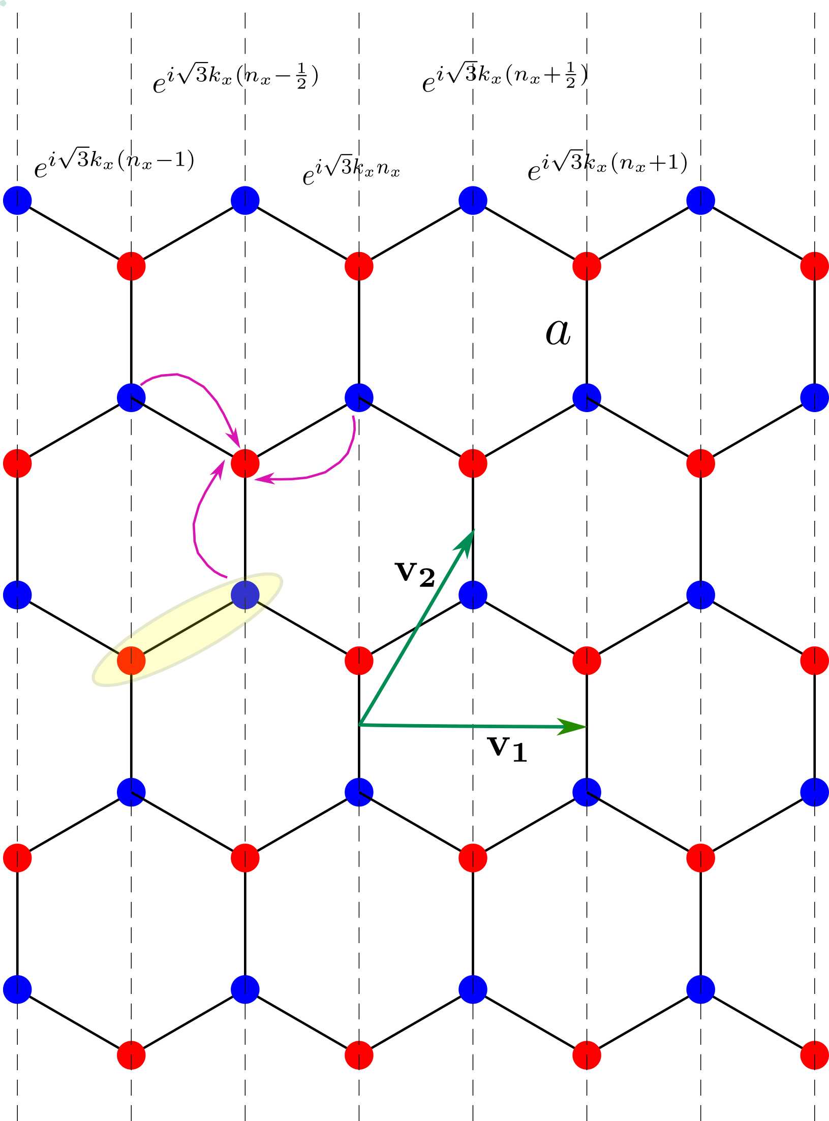
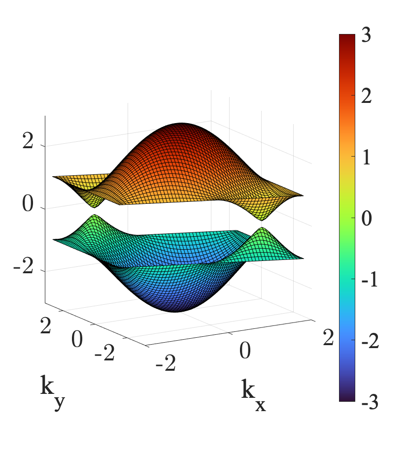
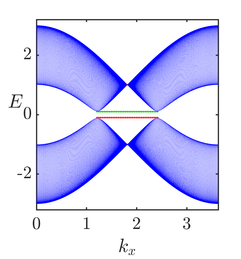
Figure 1: (a) A honeycomb lattice is a triangular lattice with a two-site unit cell of type $A$ (red) and $B$ (blue). The spanning vectors of the underlying triangular lattice are given by green arrows $\bf{v_{1}}$ and $\bf{v_{2}}$. The pink arrows show the nearest neighbor hoppings. Note that the zigzag edge is parallel to the $x-$direction. The bottom edge of the ribbon has sites of type $A$ whereas the top edge has sites of type $B$. (b) The bulk spectrum in presence of a staggered potential $\mu_{s}$, has a band gap $\delta E=2\mu_{S}$ at the $K$ and $K^{\prime}$ points. (c) The edge state spectrum shows that there are edge modes (red at top edge and green at bottom edge) which are not robust.

III Elliptically polarized light

The most general form of the time-dependent vector potential of elliptically polarized light is given by

$$\bf{A}(t) = (A_{0x}\cos(\Omega t),A_{0y}\cos(\Omega t+\phi_{0})).$$ (7)

Here $\phi_{0}$ denotes the phase difference between the $x$ and $y$ components of the time-dependent fields. The electric field is therefore written as,

$${\bf E}(t)=-\frac{\partial{\bf A}}{\partial t}=(E_{0x}\sin(\Omega t),E_{0y}\sin(\Omega t+\phi_{0})),$$ (8)

where $E_{0x(y)}=\Omega A_{0x(y)}$. We note that both linear and circular polarization are special cases of Eq. (8).

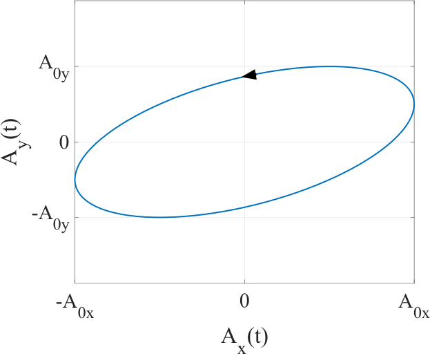
(a) $\phi_{0}=\pi/3$

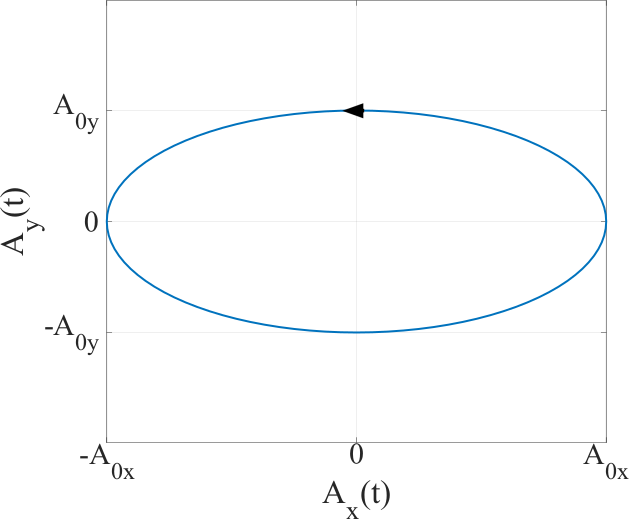
(b) $\phi_{0}=\pi/2$

Figure 2: The polarization ellipse for two values of the phase $\phi_{0}$ (a)$\pi/3$ and (b)$\pi/2$. Clearly, when $\phi_{0}=\pm\pi/2$, the axes of the ellipse are parallel to the $x$ and $y-$directions. The special case of $A_{0x}=A_{0y}$ with $\phi_{0}=\pm\pi/2$ gives left(right) circular polarization. For other values of $\phi_{0}$ the ellipse is rotated. In both these figures we have taken $A_{0x}=0.7$ and $A_{0y}=0.4$. The ratio of these amplitudes decides the “flatness” of the ellipse. The ellipticity or eccentricity of the ellipse depends both on the ratio of amplitudes and the phase.

Figure 2 shows the polarization ellipses for two choices of parameters. Fixing $\phi_{0}=\pm\pi/2$, we obtain elliptically polarized light with the axes of the ellipse aligned with the cardinal axes as shown in Fig. 2(b). Further, if $A_{0x}=A_{0y}$ and $\phi_{0}=\pm\pi/2$, we obtain left/right circularly polarized light. While the ratio $A_{0x}/A_{0y}$ decides the “flatness” of the ellipse, the ellipticity depends on this ratio as well as the phase.

The vector potential given by Eq. (7) enters the momentum-space Hamiltonian via minimal coupling, ${\bf k}\longrightarrow{\bf k}+{\bf A}$. Therefore, the bulk Hamiltonian in Eq. (2) is modified as $h({\bf k})\longrightarrow h({\bf k}+{\bf A})$.

IV Floquet topological phases

Now we use the form of the perturbation described in Sec. III to drive the honeycomb lattice out of equilibrium. We employ Floquet theory to study this since the drive is assumed to be perfectly periodic in time. Consider a time-dependent Hamiltonian $H(t)$ with periodicity $T=2\pi/\Omega$ i.e.,

$$H(t)=H(t+T),$$ (9)

where $\Omega$ is the frequency associated with the driven system. According to Floquet theorem [29, 41], the solutions to the time-dependent Schrödinger equation (setting $\hbar=1$)

$$\Big{(}H(t)-i\frac{\partial}{\partial t}\Big{)}\Psi(t)=0,$$ (10)

are given by

$$\psi_{\alpha}(t)=e^{-i\epsilon_{\alpha}t}\phi_{\alpha}(t),$$ (11)

where the quasienergy $\epsilon_{\alpha}$ is unique modulo $n\Omega$, i.e.

$$\epsilon_{\alpha}\equiv\epsilon_{\alpha}+n\Omega,~{}~{}~{}~{}n=0,\pm 1\pm 2...$$ (12)

This means that now there are multiple copies of each band. The two bands with $n=0$ lie in the range $-\pi<\epsilon_{\alpha}T<\pi$ and are called the “primary Floquet bands”, while the copies of these bands lying outside this energy range are the “side bands”. Note that this is analogous to the concept of Brillouin Zone in Bloch theory where the periodicity on a real space lattice gives rise to a Bloch momentum; similarly in Floquet theory the periodicity in time is reflected in the quasienergy spectrum. The state $\phi_{\alpha}(t)$ is periodic with the same time period as the Hamiltonian $H(t)$, i.e,

$$\phi_{\alpha}(t)=\phi_{\alpha}(t+T).$$ (13)

The time evolution operator from an earlier time $t_{1}$ to a later time $t_{2}$ is defined as

$$\mathcal{U}(t_{2},t_{1})=\mathfrak{T}e^{-i\int_{t_{1}}^{t_{2}}dtH(t)},$$ (14)

where $\mathfrak{T}$ denotes time ordering and is essential, since the hamiltonians at two different times do not, in general, commute with each other. In particular, for exactly one drive cycle, this time-evolution operator is called the Floquet operator, i.e.,

$$\mathcal{U}_{T}=\mathcal{U}(T,0)=\mathfrak{T}e^{-i\int_{0}^{T}dtH(t)}.$$ (15)

Since $\psi(t+T)=\mathcal{U}_{T}\psi(t)$, from Eq. (11),

$$\mathcal{U}_{T}\psi_{\alpha}=e^{-i\epsilon_{\alpha}T}\psi_{\alpha}.$$ (16)

We can then use the Floquet eigenstates $\psi_{\alpha}$s thus obtained to find the Chern numbers according to the prescription in App. A for various drive parameters. We fix the drive frequency at $\Omega=3$ in units of the hopping parameter $\gamma$, which is much larger than the band gap of the unperturbed system. We then plot the Chern number of the upper band (in the primary Floquet zone) as a function of the drive amplitudes $A_{0x}$ and $A_{0y}$ for various values of the phase $\phi$. This gives rise to the phase diagrams of Fig. 3. An interesting feature of these phase diagrams is the absence of reflection symmetry about the $A_{0x}=A_{0y}$ line for any value of $\phi_{0}$. This is strikingly different from the case of the driven Bernevig-Hughes-Zhang (BHZ) model [31] where the corresponding Floquet topological phase diagram has the aforementioned reflection symmetry. The reason for this is that the BHZ model is constructed from a square lattice while the honeycomb lattice has a hexagonal structure for which the Hamiltonian does not transform trivially under $k_{x}\leftrightarrow k_{y}$.

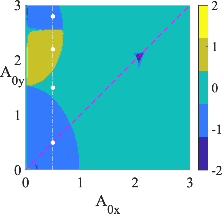
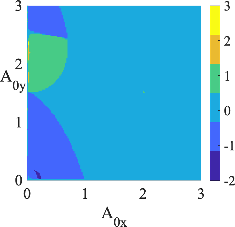
Figure 3: Phase diagram showing the Chern numbers $C_{+}$ of the top band as a function of drive amplitudes for two different values of the phase (a) $\phi=\pi/2$ and (b)$\phi=\pi/3$. We take the staggered potential $\mu_{s}=0.001$ i.e., we start from a gapped but trivial phase and drive using a frequency $\Omega=3$ which is much larger than the band gap of the spectrum of the unperturbed system. The pink dashed line $A_{0x}=A_{0y}$ in (a) is the special case of circularly polarized light. The vertical white dot-dash line goes through four different phases by keeping $A_{0x}$ constant and varying $A_{0y}$. The four dots on this line correspond to the parameters chosen to study the edge state spectrum in Fig. 4.

V Edge modes

Next we verify the bulk boundary correspondence for the phases in Fig. 3. For this, we again consider a nanoribbon which is infinite along the $x-$direction i.e. along the zigzag edge as shown in Fig.1. Since now we are studying the effect of a polarized light, we use minimal coupling and Peierls substitution to modify the momentum and the hopping parameter respectively as,

$$k_{x} \rightarrow k_{x}+A_{0x}\cos(\Omega t),$$

$$\gamma \rightarrow \gamma~{}e^{i\bf{A(t)}.\bf{r}},$$ (17)

where $\bf{r}$ is the vector joining the two sites between which hopping is being considered. This modifies the Hamiltonian for a nanoribbon as

$$h^{1D}(k_{x},t) = \gamma\sum_{n_{y}}\Big{[}a_{n_{y}}^{\dagger}b_{n_{y}-1}e^{-iA_{y}(t)}+2\cos{\frac{\sqrt{3}(k_{x}+A_{x}(t))}{2}}a_{n_{y}}^{\dagger}b_{n_{y}}e^{i\frac{A_{y}(t)}{2}}\Big{]}.$$ (18)

We then use the above Hamiltonian to construct the time evolution operator for this one-dimensional chain, diagonalizing which gives us Floquet eigenvalues and eigenstates. The quasienergy spectrum thus obtained is shown in Fig. 4.

(a) $A_{0x}=0.5,A_{0y}=0.5$

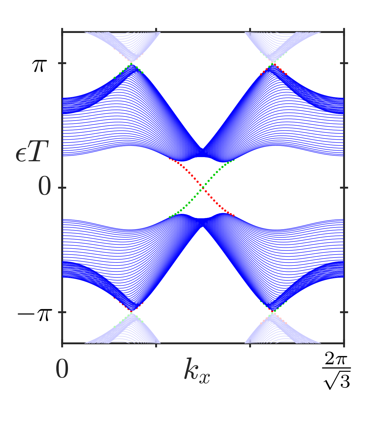
(b) $A_{0x}=0.5,A_{0y}=1.6$

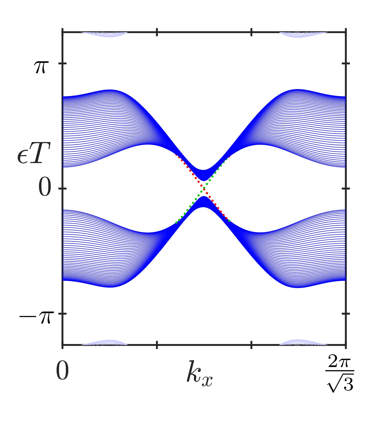
(c) $A_{0x}=0.5,A_{0y}=2.2$

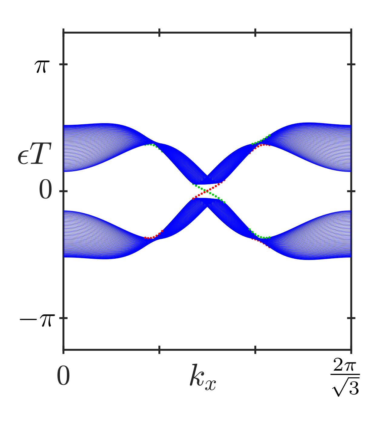
(d) $A_{0x}=0.5,A_{0y}=2.6$

Figure 4: Edge state spectra for different ratios of the drive amplitudes while keeping the frequency $\Omega=3$ and phase $\phi_{0}=\pi/2$ fixed. These correspond to the four points marked along the white line in Fig. 2(a). The red and green colors correspond to states localized at the bottom and top edge respectively.

We find that the number of edge states are consistent with the Floquet Chern numbers in the phase diagram of Fig. 3. To see this we fix $\phi_{0}=\pi/2$ and $A_{0x}=0.5$ and choose values of $A_{0y}$ in the four different phases of Fig.3. The magnitude of the Chern number counts the number of edge modes while the sign indicates the chirality, i.e. the direction of propagation. In Fig. 4(a), we find one pair of edge states at $\epsilon T=0$ and two pairs at $\epsilon T=\pm\pi$. These have opposite directions of propagation i.e. at $\epsilon T=0$ we have a top edge right mover while at $\epsilon T=\pm\pi$ we have two top edge left movers. These add up to give a Chern number $C_{+}=-1$. In Fig. 4(b) we seem to have edge states. However there is no gap at $\epsilon T=\pm\pi$ which makes the system trivial. In Fig.4(c) we find a top edge right mover corresponding to a Chern number $C_{+}=+1$, whereas in Fig.4(d) we have a top edge left mover corresponding to a Chern number $C_{+}=-1$.

VI Conclusions and Outlook

We have studied the Floquet topological phases generated by driving a honeycomb lattice such as graphene out of equilibrium by using polarized light. However, we consider the most general case of elliptically polarized light. Some of the effects of such a time-dependent perturbation are markedly different from the more commonly studied cases of linear or circular polarization. In particular, a rich topological phase diagram is generated with Chern numbers depending on both the phase $\phi_{0}$ and the ratio $A_{0x}/A_{0y}$. Keeping $\phi_{0}$ fixed and varying this ratio allows us to tune in and out of topological phases. We also find that the chiral edge modes on a nanoribbon of this driven system are consistent with the Floquet Chern numbers obtained from the bulk.

While this system with its rich phase diagram is by itself quite interesting, another aspect to consider is the effect of spin-orbit coupling on such a system. For instance, it is well known that a Kane-Mele type SOC makes the equilibrium honeycomb lattice topological. The interplay of this SOC with an external perturbation using elliptically polarized light could lead to an even richer phase diagram and could allow us to engineer topological phases with higher Chern numbers.

This work is restricted to studying the topological properties of the Floquet bands that arise as a result of periodically driving the electrons on a honeycomb lattice. However, due to the fact that there are infinitely many copies of these bands corresponding to different integer values of $n$, the occupation of these bands is very different from a conventional Fermi distribution. The effect of this distribution in the out-of-equilibrium system is expected to play a pivotal role in observable properties of the material such as the longitudinal and transverse conductance which are directly related to the topological nature of the system.

Appendix A Numerical evaluation of Chern number

Given a hamiltonian $h({\bf k})$, the eigenvalue equation is given by

$$h({\bf k})|\psi_{\alpha}({\bf k})\rangle=E_{\alpha}({\bf k})|\psi_{\alpha}({\bf k})\rangle$$ (19)

with $|\psi_{\alpha}({\bf k})\rangle$ being the eigenstate corresponding to eigenvalue $E_{\alpha}$. In the model we have considered $\alpha=\pm$ corresponds to the upper/lower bands and $|\psi_{\alpha}({\bf k})\rangle$s are two-component spinors. However, note that the discussion that follows holds good for any $n-$band system (in which case each eigenstate is an $n-$component spinor).

The eigenstates $|\psi_{\alpha}({\bf k})\rangle$ are then used to define the Berry curvature, and the Chern number of the $\alpha$th band as

$$C_{\alpha}=~{}\frac{i}{2\pi}~{}\int\int dk_{x}dk_{y}\Big{[}~{}\frac{\partial\psi_{\alpha}^{\dagger}}{\partial k_{x}}\frac{\partial\psi_{\alpha}}{\partial k_{y}}-\frac{\partial\psi_{\alpha}^{\dagger}}{\partial k_{y}}\frac{\partial\psi_{\alpha}}{\partial k_{x}}\Big{]}.$$ (20)

When we numerically evaluate $|\psi_{\alpha}\rangle$ there is an arbitrary phase factor which is included thereby making the direct numerical computation of he above expression complicated. We need a method to calculate this which is gauge-invariant, i.e. independent of the arbitrary phase factor which can always multiply the eigenvector. Therefore we resort to the method similar to Fukui et. al. [42].

Consider an actual numerical computation where the eigenvectors are evaluated on a discretized two-dimensional Brillouin Zone (B.Z). We denote the points on the momentum mesh as $(n_{x},n_{y})$ with $n_{x}\in[1,N_{x}],n_{y}\in[1,N_{y}]$. The $\alpha$th eigenvector at each such momentum point is written as $|\psi_{\alpha,n_{x},n_{y}}\rangle$. Four consecutive $k-$points on this momentum mesh form a plaquet. We define a variable $F_{\alpha,n_{x},n_{y}}$ associated with this plaquet as

$$F_{\alpha,n_{x},n_{y}}$$

$$= \ln\Bigg{[}\frac{\langle\psi_{\alpha,n_{x},n_{y}}|\psi_{\alpha,n_{x}+1,n_{y}}\rangle}{|\langle\psi_{\alpha,n_{x},n_{y}}|\psi_{\alpha,n_{x}+1,n_{y}}\rangle|}\frac{\langle\psi_{\alpha,n_{x}+1,n_{y}}|\psi_{\alpha,n_{x}+1,n_{y}+1}\rangle}{|\langle\psi_{\alpha,n_{x}+1,n_{y}}|\psi_{\alpha,n_{x}+1,n_{y}+1}\rangle|}\frac{\langle\psi_{\alpha,n_{x}+1,n_{y}+1}|\psi_{\alpha,n_{x},n_{y}+1}\rangle}{|\langle\psi_{\alpha,n_{x}+1,n_{y}+1}|\psi_{\alpha,n_{x},n_{y}+1}\rangle|}\frac{\langle\psi_{\alpha,n_{x},n_{y}+1}|\psi_{\alpha,n_{x},n_{y}}\rangle}{|\langle\psi_{\alpha,n_{x},n_{y}+1}|\psi_{\alpha,n_{x},n_{y}}\rangle|}\Bigg{]}.$$

Note that we use only the principal branch of the logarithm function in Eq. A. Summing this over the entire B.Z. gives the Chern number of the $\alpha$th band, which is an integer

$$C_{\alpha}=\frac{1}{2i\pi}\sum_{n_{x},n_{y}}F_{\alpha,n_{x},n_{y}}.$$ (22)

References

- Kou et al. [2013] L. Kou, B. Yan, F. Hu, S.-C. Wu, T. O. Wehling, C. Felser, C. Chen, and T. Frauenheim, Graphene-based topological insulator with an intrinsic bulk band gap above room temperature, Nano Letters 13, 6251 (2013), https://doi.org/10.1021/nl4037214 .
- Zhang et al. [2014] J. Zhang, C. Triola, and E. Rossi, Proximity effect in graphene–topological-insulator heterostructures, Phys. Rev. Lett. 112, 096802 (2014).
- Zollner et al. [2016] K. Zollner, T. Frank, S. Irmer, M. Gmitra, D. Kochan, and J. Fabian, Spin-orbit coupling in methyl functionalized graphene, Phys. Rev. B 93, 045423 (2016).
- Hasan and Kane [2010] M. Z. Hasan and C. L. Kane, Colloquium: Topological insulators, Rev. Mod. Phys. 82, 3045 (2010).
- Bernevig et al. [2006] B. A. Bernevig, T. L. Hughes, and S.-C. Zhang, Quantum spin hall effect and topological phase transition in hgte quantum wells, Science 314, 1757 (2006).
- Moore [2010] J. E. Moore, The birth of topological insulators, Nature 464, 194 (2010).
- Moore and Balents [2007] J. E. Moore and L. Balents, Topological invariants of time-reversal-invariant band structures, Phys. Rev. B 75, 121306 (2007).
- Fu et al. [2007] L. Fu, C. L. Kane, and E. J. Mele, Topological insulators in three dimensions, Phys. Rev. Lett. 98, 106803 (2007).
- Kitagawa et al. [2010] T. Kitagawa, E. Berg, M. Rudner, and E. Demler, Topological characterization of periodically driven quantum systems, Phys. Rev. B 82, 235114 (2010).
- Kitagawa et al. [2011] T. Kitagawa, T. Oka, A. Brataas, L. Fu, and E. Demler, Transport properties of nonequilibrium systems under the application of light: Photoinduced quantum hall insulators without landau levels, Phys. Rev. B 84, 235108 (2011).
- Oka and Aoki [2009] T. Oka and H. Aoki, Photovoltaic hall effect in graphene, Phys. Rev. B 79, 081406 (2009).
- Gu et al. [2011] Z. Gu, H. A. Fertig, D. P. Arovas, and A. Auerbach, Floquet spectrum and transport through an irradiated graphene ribbon, Phys. Rev. Lett. 107, 216601 (2011).
- Lindner et al. [2011] N. H. Lindner, G. Refael, and V. Galitski, Floquet topological insulator in semiconductor quantum wells, Nature Physics 7, 490 (2011).
- Suárez Morell and Foa Torres [2012] E. Suárez Morell and L. E. F. Foa Torres, Radiation effects on the electronic properties of bilayer graphene, Phys. Rev. B 86, 125449 (2012).
- Kundu et al. [2014] A. Kundu, H. A. Fertig, and B. Seradjeh, Effective theory of floquet topological transitions, Phys. Rev. Lett. 113, 236803 (2014).
- Dóra et al. [2012] B. Dóra, J. Cayssol, F. Simon, and R. Moessner, Optically engineering the topological properties of a spin hall insulator, Phys. Rev. Lett. 108, 056602 (2012).
- Thakurathi et al. [2013] M. Thakurathi, A. A. Patel, D. Sen, and A. Dutta, Floquet generation of majorana end modes and topological invariants, Phys. Rev. B 88, 155133 (2013).
- Katan and Podolsky [2013] Y. T. Katan and D. Podolsky, Modulated floquet topological insulators, Phys. Rev. Lett. 110, 016802 (2013).
- Zhu et al. [2014] H.-X. Zhu, T.-T. Wang, J.-S. Gao, S. Li, Y.-J. Sun, and G.-L. Liu, Floquet topological insulator in the BHZ model with the polarized optical field, Chinese Physics Letters 31, 030503 (2014).
- Rudner et al. [2013] M. S. Rudner, N. H. Lindner, E. Berg, and M. Levin, Anomalous edge states and the bulk-edge correspondence for periodically driven two-dimensional systems, Phys. Rev. X 3, 031005 (2013).
- Nathan and Rudner [2015] F. Nathan and M. S. Rudner, Topological singularities and the general classification of floquet–bloch systems, New Journal of Physics 17, 125014 (2015).
- Carpentier et al. [2015] D. Carpentier, P. Delplace, M. Fruchart, and K. Gawedzki, Topological index for periodically driven time-reversal invariant 2d systems, Phys. Rev. Lett. 114, 106806 (2015).
- Xiong et al. [2016] T.-S. Xiong, J. Gong, and J.-H. An, Towards large-chern-number topological phases by periodic quenching, Phys. Rev. B 93, 184306 (2016).
- Thakurathi et al. [2017] M. Thakurathi, D. Loss, and J. Klinovaja, Floquet majorana fermions and parafermions in driven rashba nanowires, Phys. Rev. B 95, 155407 (2017).
- Mukherjee et al. [2018] B. Mukherjee, P. Mohan, D. Sen, and K. Sengupta, Low-frequency phase diagram of irradiated graphene and a periodically driven spin- xy chain, Phys. Rev. B 97, 205415 (2018).
- Zhou and Gong [2018] L. Zhou and J. Gong, Recipe for creating an arbitrary number of floquet chiral edge states, Phys. Rev. B 97, 245430 (2018).
- López et al. [2012] A. López, Z. Z. Sun, and J. Schliemann, Floquet spin states in graphene under ac-driven spin-orbit interaction, Phys. Rev. B 85, 205428 (2012).
- Zhang et al. [2016] X.-X. Zhang, T. T. Ong, and N. Nagaosa, Theory of photoinduced floquet weyl semimetal phases, Phys. Rev. B 94, 235137 (2016).
- Floquet [1883] G. Floquet, On linear differential equations with periodic coefficients, Scientific annals of the Ecole Normale Supérieure 2nd series, 12, 47 (1883).
- Trevisan et al. [2022] T. V. Trevisan, P. V. Arribi, O. Heinonen, R.-J. Slager, and P. P. Orth, Bicircular light floquet engineering of magnetic symmetry and topology and its application to the dirac semimetal , Phys. Rev. Lett. 128, 066602 (2022).
- Seshadri and Sen [2022] R. Seshadri and D. Sen, Engineering floquet topological phases using elliptically polarized light, Phys. Rev. B 106, 245401 (2022).
- Kitayama et al. [2021] K. Kitayama, Y. Tanaka, M. Ogata, and M. Mochizuki, Floquet theory of photoinduced topological phase transitions in the organic salt -(bedt-ttf)2i3 irradiated with elliptically polarized light, Journal of the Physical Society of Japan 90, 104705 (2021), https://doi.org/10.7566/JPSJ.90.104705 .
- Baykusheva et al. [2021] D. Baykusheva, A. Chacón, J. Lu, T. P. Bailey, J. A. Sobota, H. Soifer, P. S. Kirchmann, C. Rotundu, C. Uher, T. F. Heinz, D. A. Reis, and S. Ghimire, All-optical probe of three-dimensional topological insulators based on high-harmonic generation by circularly polarized laser fields, Nano Letters 21, 8970 (2021), pMID: 34676752, https://doi.org/10.1021/acs.nanolett.1c02145 .
- Chnafa et al. [2021] H. Chnafa, M. Mekkaoui, A. Jellal, and A. Bahaoui, Effect of strain on band engineering in gapped graphene, The European Physical Journal B 94, 39 (2021).
- Díaz-Fernández [2020] A. Díaz-Fernández, Inducing anisotropies in dirac fermions by periodic driving, Journal of Physics: Condensed Matter 32, 495501 (2020).
- Bernvig et al. [2006] B. A. Bernvig, T. L. Hughes, S.-C. Zhang, H.-D. Chen, and C. Wu, Band collapse and the quantum hall effect in graphene, International Journal of Modern Physics B 20, 3257 (2006).
- Semenoff [1984] G. W. Semenoff, Condensed-matter simulation of a three-dimensional anomaly, Phys. Rev. Lett. 53, 2449 (1984).
- Kane and Mele [2005] C. L. Kane and E. J. Mele, Quantum spin hall effect in graphene, Phys. Rev. Lett. 95, 226801 (2005).
- Seshadri et al. [2016] R. Seshadri, K. Sengupta, and D. Sen, Edge states, spin transport, and impurity-induced local density of states in spin-orbit coupled graphene, Phys. Rev. B 93, 035431 (2016).
- Seshadri and Sen [2017] R. Seshadri and D. Sen, Electron dynamics in graphene with spin–orbit couplings and periodic potentials, Journal of Physics: Condensed Matter 29, 155303 (2017).
- Holthaus [2015] M. Holthaus, Floquet engineering with quasienergy bands of periodically driven optical lattices, Journal of Physics B: Atomic, Molecular and Optical Physics 49, 013001 (2015).
- Fukui et al. [2005] T. Fukui, Y. Hatsugai, and H. Suzuki, Chern numbers in discretized brillouin zone: Efficient method of computing (spin) hall conductances, Journal of the Physical Society of Japan 74, 1674 (2005).