Equilibrium behaviour of two cavity-confined polymers: Effects of polymer width and system asymmetries

Abstract

Experiments using nanofluidic devices have proven effective in characterizing the physical properties of polymers confined to small cavities. Two recent studies using such methods examined the organization and dynamics of two DNA molecules in box-like cavities with strong confinement in one direction and with square and elliptical cross sections in the lateral plane. Motivated by these experiments, we employ Monte Carlo and Brownian dynamics simulations to study the physical behaviour of two polymers confined to small cavities with shapes comparable to those used in the experiments. We quantify the effects of varying the following polymer properties and confinement dimensions on the organization and dynamics of the polymers: the polymer width, the polymer contour length ratio, the cavity cross-sectional area, and the degree of cavity elongation for cavities with rectangular and elliptical cross sections. We find that the tendency for polymers to segregate is enhanced by increasing polymer width. For sufficiently small cavities, increasing cavity elongation promotes segregation and localization of identical polymers to opposite sides of the cavity along its long axis. A free-energy barrier controls the rate of polymers swapping positions, and the observed dynamics are roughly in accord with predictions of a simple theoretical model. Increasing the contour length difference between polymers significantly affects their organization in the cavity. In the case of a large linear polymer co-trapped with a small ring polymer in an elliptical cavity, the small polymer tends to lie near the lateral confining walls, and especially at the cavity poles for highly elongated ellipses.

I Introduction

Confinement of a polymer chain to a sufficiently small space significantly affects its size and shape as well as its dynamical properties. The resulting conformational distortion tends to enhance the entropic repulsion between different polymer chains, thus reducing interchain overlap and promoting chain segregation. A well studied case is confinement of multiple polymers to long cylindrical channels and cylindrical cavities of finite length. Numerous computer simulation studies have examined the effects of entropic repulsion for two polymers in such geometries.Jun and Mulder (2006); Teraoka and Wang (2004); Jun et al. (2007); Arnold and Jun (2007); Jacobsen (2010); Jung and Ha (2010); Jung et al. (2012a, b); Liu and Chakraborty (2012); Dorier and Stasiak (2013); Račko and Cifra (2013); Shin et al. (2014); Minina and Arnold (2014, 2015); Chen et al. (2015); Polson and Montgomery (2014); Du et al. (2018); Polson and Kerry (2018); Nowicki (2019a, b); Polson and Zhu (2021); Mitra et al. (2022a, b) Most of these studies have examined the segregation behaviour of flexible linear polymers,Jun and Mulder (2006); Teraoka and Wang (2004); Jun et al. (2007); Arnold and Jun (2007); Jacobsen (2010); Jung and Ha (2010); Jung et al. (2012b); Liu and Chakraborty (2012); Račko and Cifra (2013); Minina and Arnold (2014); Polson and Montgomery (2014); Du et al. (2018) though some have also investigated the behaviour of ring polymersJung et al. (2012a); Dorier and Stasiak (2013); Shin et al. (2014); Minina and Arnold (2015); Chen et al. (2015); Polson and Kerry (2018) and more complex topologies.Mitra et al. (2022a, b) In addition, the effects of bending rigidity,Račko and Cifra (2013); Polson and Montgomery (2014) a difference in the contour lengths,Polson and Zhu (2021) macromolecular crowding,Shin et al. (2014); Chen et al. (2015); Polson and Kerry (2018) and electrostaticsNowicki (2019a, b) on the segregation dynamics and thermodynamics have been examined in detail. Information gleaned from these studies may be useful in helping advance nanofluidic technology used in applications such as DNA sorting,Dorfman et al. (2012) DNA denaturation mapping,Reisner et al. (2010); Marie et al. (2013) and genome mapping.Lam et al. (2012); Hastie et al. (2013); Dorfman (2013); Müller and Westerlund (2017) The degree to which polymers either mix or partition in such nanofluidic devices may impact their performance in cases where the devices are operated at high polymer concentrations to increase throughput.

Understanding the behaviour of confined polymers may also help elucidate the role of entropy in the segregation of replicating chromosomes of prokaryotes into the daughter cells. Some bacteria such as E. coli possess no known active machinery to promote segregation, and it has been proposed that entropy provides the key driving force in such systems.Jun and Mulder (2006); Jun and Wright (2010); Di Ventura et al. (2013); Youngren et al. (2014); Mannik et al. (2016) In this scenario, confinement-enhanced entropic repulsion between chromosomes pushes them apart along the long axis of the rod-shaped cells in a manner comparable to the process observed for two channel-confined polymers in various simulation studies. Several recent experimental studies have reported supporting evidence for such a mechanism.Di Ventura et al. (2013); Mannik et al. (2016); Cass et al. (2016); Wu et al. (2019, 2020); El Najjar et al. (2020); Japaridze et al. (2020); Liang et al. (2020); Gogou et al. (2021) For example, Wu et al. Wu et al. (2020) found that segregation defects observed in cell-wall-less states of Bacillus subtilis could be eliminated by confining the cells to narrow channels, which promoted successful segregation by recovering the elongated cell shape. Likewise, Liang et al. studied chromosome segregation in E. coli confined to microchannels of variable width and found the efficiency of chromosome segregation increases appreciably as the channel narrows. As simulations show that the entropic driving force increases with decreasing channel width Polson and Montgomery (2014); Polson and Kerry (2018); Polson and Zhu (2021) the experiments clearly support models of cell division in which entropy plays a prominent role in prokaryotic chromosome segregation.

While simulation studies of polymer segregation provide some degree of insight into experimental measurements of bacterial chromosome segregation, direct quantitative comparison is difficult. Bacterial chromosomes are highly complex structures packed into a crowded environment, and their detailed physical behaviour is difficult to capture using the simplistic bead-spring-type models that computer simulations typically employ. Fortunately, a much cleaner experimental test of theoretical predictions and simulation results for such systems is possible using nanofluidic devices. Recent advances in nanofabrication techniques have facilitated the construction of devices that are ideal for trapping and manipulating individual polymers. For example, nanotopography features such as ‘nanopits’ can be embedded in one surface of a nanoslit and function as entropic traps for polymers confined to the slit. Such devices can be used to manipulate polymer chains in various ways. For example, recent studies by Klotz et al. used fluorescence microscopy to examine the behaviour of single DNA chains confined to such a complex geometry and observed polymer contour sharing between multiple adjacent nanopits in a ‘tetris’-like conformation.Klotz et al. (2015a, b) Alternatively, active nanofluidic approaches, such as the Convex-lens Induced ConfinementBerard et al. (2014) can be used to dynamically adjust the slit width, creating a top-loading effect whereby entire molecules can be driven inside the nanopits.

Recently, Reisner and coworkers employed a top-loading version of a nanofluidic structure using pneumatically activated nanoscale nitride membranes.Capaldi et al. (2018); Liu et al. (2022) This mechanism was used to trap fluorescently stained DNA molecules into the cavities formed by sealing off the nanopits. In some cases, single molecules were trapped, and in other cases pairs of DNA molecules were trapped. Using a mixture of DNA molecules stained with two different dyes, some cavities contained two DNA molecules that were visually distinguishable by colour, thus facilitating the observation and characterization of the organization and dynamics of the individual chains. The simplicity of the systems used in such in vitro experiments provide results that are much more amenable to direct quantitative comparison with computer simulations employing simple models than are the in vivo experiments studying bacterial chromosome segregation.

The studies of Refs. Capaldi et al., 2018 and Liu et al., 2022 employed cavities in which the DNA molecules are strongly confined in one dimension and much less so in the lateral dimensions. In each case, the cavity height of 200 nm is appreciably smaller than the bulk radius of gyration of the linear DNA molecules used (0.7 $\mu$m for $\lambda$ DNA), thus compressing the chains in that dimension and enhancing repulsion in the lateral plane. Ref. Capaldi et al., 2018 employed cavities with a square cross section of side length 2 $\mu$m, while Ref. Liu et al., 2022 employed cavities with elliptical cross sections of fixed cross-sectional area and variable eccentricity, $e$, with maximum diameter ranging from 2 $\mu$m ($e=0$) to 3 $\mu$m ($e=0.9$). Such values are comparable to the lateral extent of singly-trapped $\lambda$ DNA molecules, thus ensuring that two co-trapped molecules will interact strongly with each other.

In the case of square cavities,Capaldi et al. (2018) the presence of a second $\lambda$ DNA molecule had a pronounced effect on both the position probability distribution and the chain dynamics. Entropic repulsion tended to push the molecules apart and away from the cavity centre, the most probable location for single-chain trapping. This effect was also observed, somewhat more weakly, when the $\lambda$ DNA chain was trapped with a much smaller plasmid. In addition, the $\lambda$-DNA dynamics were slowed when a second chain was trapped, much more so in the case where the second chain is $\lambda$ DNA than for a plasmid. In the former case, the authors of Ref. Capaldi et al., 2018 infer a “Brownian rotor” collective motion of the two chains. They also observed an asymmetry in the lateral centre-of-mass position distributions for two-chain systems where the $\lambda$ DNA molecules are stained with different dyes. This likely arises because the two dyes (YOYO-1 and YOYO-3) unwind the double helix by different amounts leading to different contour lengths. In the case of elliptical cavities,Liu et al. (2022) elongating the cavity by increasing its eccentricity increased the tendency for two co-trapped $\lambda$ DNA molecules to segregate to the poles of the ellipse and decreased the rate with which the two chains swap positions. Liu et al. also investigated the behaviour of a single plasmid trapped with a T₄ DNA molecule in an elliptical cavity. They found that entropic repulsion with the T₄ DNA chain enhanced the probability of the plasmid lying near the lateral walls, and increasingly so at the poles of the ellipse as the eccentricity was increased.

The nanocavity-confined DNA systems studied in Refs. Capaldi et al., 2018 and Liu et al., 2022 are simple enough to benefit from complementary studies using computer simulations with simple molecular models. Recently, we used Brownian dynamics and Monte Carlo simulation methods to study the organization and dynamics of two flexible Lennard-Jones chains trapped in cavities resembling those with square cross sections used in Ref. Capaldi et al., 2018.Polson and Rehel (2021) We calculated the position probability distributions in the lateral plane and the centre-of-mass dynamics and measured their variation with lateral box size and polymer length. As in the experiments, the behaviour of the system was drastically altered by the presence of the second polymer, and was also highly sensitive to the cavity size. In smaller boxes the dynamical behaviour of the system was slowed due to the presence of the second polymer. The centre-of-mass dynamics were readily interpreted using the lateral position probability distributions. Generally, the results were qualitatively consistent with those of the experimental study of Capaldi et al.Capaldi et al. (2018) However, the simulation results were not suitable for a direct quantitative comparison with experiment. Because of the time-consuming nature of the dynamics calculations, the polymer chains were limited to lengths of $\lesssim 100$ monomers, which effectively results in an artificially large value of the polymer width relative to the persistence and contour lengths when the model is mapped onto $\lambda$ DNA. In addition, the presumed asymmetry in the contour lengths of the differentially stained DNA molecules was not incorporated into the model.

In this study, we build on our previous work in Ref. Polson and Rehel, 2021 and use Monte Carlo (MC) and Brownian dynamics (BD) simulations to study systems of two polymers entrapped in cavities of comparable shape and size as those used in the experiments. We address issues arising from the previous study by incorporating features that improve the semblance of the molecular model to the DNA systems studied in Ref. Capaldi et al., 2018. This includes using more realistic values for the effective polymer width as well employing different polymer contour lengths for each of the two polymers. Generally, we find that reducing the effective width also reduces the strength of interchain repulsion, thus diminishing the tendency for polymer segregation. Confinement of polymers of different contour length effects an asymmetry in the position probability distribution qualitatively similar to that seen in the experiments. We also examine the effects of cavity elongation in the lateral plane, employing rectangular cross sections as well as the elliptical cross sections used in Ref. Liu et al., 2022. As in the experiments, we find that for sufficiently small cavities, increasing the elongation enhances segregation of the polymers along the long symmetry axis. In addition, the free energy barrier that governs chain swapping grows, leading to a reduced swapping frequency, in accord with the experiments. A small ring polymer trapped in an elliptical cavity with large linear polymer tends to locate near the poles of the ellipse as a result of enhanced entropic depletion of the linear polymer in these regions, an effect also observed in experiments using a small plasmid entrapped with a T₄ DNA molecule.Liu et al. (2022)

The remainder of this article is organized as follows. Section II provides a description of the two polymer models employed in the MC and BD simulations. Section III gives an outline of the methodology used together with the relevant details of the simulations. Section IV presents the simulation results for the various systems. Finally, Sec. V summarizes the main conclusions of this work.

II Model

In this study, we examine a system of two polymers confined to a box-like cavity. The polymers are modeled as chains of spherical monomers. In most simulations, the chains are identical with $N$ monomers per chain and are of linear topology. In Sec. IV.2 we also consider polymers of unequal lengths $N_{1}$ and $N_{2}$, where we choose $N_{2}<N_{1}$, but which are otherwise identical. In Sec. IV.4 we examine a system of two chains of unequal length where one has a linear topology while the other is a ring topology. Depending on whether we use MC or BD simulations, the chain is modeled as either a semiflexible hard-sphere chain or a fully flexible chain of Lennard-Jones (LJ) monomers. The details of each are given below.

II.1 Semiflexible hard-sphere chain

In most MC simulations we employ the semiflexible hard-sphere chain model. Here, the interactions between non-bonded monomers are given by

$$u_{\rm nb}(r)=\begin{cases}\infty&r<\sigma\\ 0,&r\geq\sigma\end{cases}$$ (1)

where $r$ is distance between centres of monomers. The bond length between sequentially adjacent monomers was held fixed at a length of $\sigma$. The width $w$ of the hard-sphere polymer is defined as the diameter of each monomer, i.e., $w=\sigma$.

The bending potential for each consecutive triplet of monomers centered on monomer $i$ is given by,

$$u_{\rm bend}=\kappa(1-\cos\theta_{i}),$$ (2)

where $\cos\theta_{i}=\hat{u}_{i}\cdot\hat{u}_{i+1}$, and where $\hat{u}_{i}$ is the unit vector pointing from monomer $i-1$ to monomer $i$. The bending constant $\kappa$ determines the overall stiffness of the polymer and is related to the persistence length $P$ byMicheletti et al. (2011) $\exp(-\langle l_{\rm bond}\rangle/P)=\coth(\kappa/k_{\rm B}T)-k_{\rm B}T/\kappa$. For sufficiently large $\kappa/k_{\rm B}T$ this implies $P/\sigma\approx\kappa/k_{\rm B}T$. In this limit, the Kuhn length, $\ell_{\rm k}=2P$, therefore satisfies $\ell_{\rm k}/\sigma\approx 2\kappa/k_{\rm B}T$.

II.2 Fully flexible Lennard-Jones chain

In contrast to the hard-sphere chain model, this model employs continuous potentials and so is suitable for use in BD simulations and as well as MC simulations. Here, the non-bonded interactions are given by the repulsive LJ potential,

$$u_{\rm nb}(r)=\begin{cases}u_{\rm LJ}(r)-u_{\rm LJ}(r_{\rm c}),&r\leq r_{\rm c}\\ 0,&r>r_{\rm c}\end{cases}$$ (3)

where $u_{\text{LJ}}$ is the LJ potential,

$$u_{\text{LJ}}(r)=4\epsilon((\sigma/r)^{12}-(\sigma/r)^{6}).$$ (4)

Here, r is the distance between the centres of the two interacting monomers and, $r_{c}$=$2^{1/6}\sigma$, where $\sigma$ is the monomer diameter. The interaction between bonded monomers is given by a combination of the LJ potential given in Eq. (3) and the Finitely Extensible Non-linear Elastic (FENE) potential given by

$$u_{\text{FENE}}(r)=-\frac{1}{2}kr_{0}^{2}\ln(1-(r/r_{0})^{2}),$$ (5)

where $r_{0}$=1.5$\sigma$, and $k\sigma^{2}/\epsilon=30$. The width $w$ of the LJ polymer is defined as the diameter of each LJ monomer, i.e., $w=\sigma$.

II.3 Confinement

In all systems, the polymers were confined to a cavity with cross-sectional area $A$ in the $x-y$ plane and constant height $h$ in the $z$-direction. In most calculations, the cavity cross section was square or rectangular in shape, though elliptical cross sections were also employed in a few simulations. In the former case, the confining box-like cavity has lateral dimensions $L_{x}$ and $L_{y}$, where we choose $L_{x}\leq L_{y}$. For rectangular cross sections ($L_{x}<L_{y}$), it is convenient to define the geometric average side length $\overline{L}\equiv\sqrt{L_{x}L_{y}}$. Monomer-wall interactions were modeled by means of a virtual monomer placed at the nearest point on the wall from the actual monomer. The interaction energy is calculated using. Eq. (1) in the case of the hard-sphere chain and by Eqs. (3) and (4), in the case of the LJ chain. In each case, $r+\sigma$ is the distance between the centre of the monomer and the nearest point of interaction on the wall. Thus, the cross-sectional area, $A\equiv L_{x}L_{y}$, and height, $h$, define the space accessible to the centres of the monomers. The system is illustrated in Fig. 1.

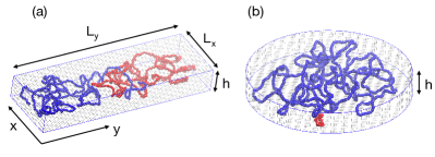
Figure 1: Illustration of the two-polymer model system. (a) Illustration of a system where the confining cavity is rectangular in shape. (b) Illustration of a system where the cavity has an elliptical cross section (see Section IV.4.) In both cases the distance $h$ between the top and bottom flat surfaces is constant.

To facilitate a comparison between simulation results and experimental results, the cavity dimensions used in the simulations are presented as ratios with respect to either the root-mean square (RMS) radius of gyration of the polymer in bulk, $R_{\rm g}$, or the RMS radius of gyration in the $x-y$ plane for a polymer confined to a slit of a given height, $R_{{\rm g},xy}$. The values of $R_{\rm g}$ and $R_{{\rm g},xy}$ for the DNA polymers employed in Refs. Capaldi et al., 2018 and Liu et al., 2022 have been measured experimentally under conditions relevant to those cavity-confinement studies.

III Methods

We use two different computer simulation methods to examine the equilibrium dynamical and non-dynamical behaviour of the system of two confined polymers. To investigate the dynamics of the centre-of-mass positions of the polymers we use BD simulations, and to examine the non-dynamical behaviour we use Metropolis MC simulations. The BD simulations can, in principle, provide the same information as the MC simulations. However, the BD simulations are significantly more time consuming, and thus we chose to use the MC simulations to obtain the non-dynamical results. A brief description of the methods is given below.

III.1 Metropolis Monte Carlo simulations

The MC simulations employ standard techniques in which a trial move is generated and accepted or rejected based on the Metropolis MC criterion. In simulations using the freely-jointed LJ chain model, we use three types of trial moves: (1) reptation moves, (2) crankshaft rotations, and (3) whole-polymer translation. In all simulations the type of trial move was randomly chosen. Each MC simulation consisted of $N_{\rm tot}\equiv N_{1}+N_{2}$ trial moves, where $N_{1}$ and $N_{2}$ are the number of monomers in each polymer. Of these moves two were whole-polymer translation, $0.9(N_{\rm tot}-2)$ were reptation, and $0.1(N_{\rm tot}-2)$ were crankshaft rotations. In the simulations using the semiflexible hard-sphere chain model, only reptation and crankshaft rotations were employed. (The exception is for the system studied in Section IV.4, where one of the polymers has a ring topology, in which case crankshaft and whole-polymer translation moves were used.) Typically, there were $0.9N_{\rm tot}$ reptation moves and $0.1N_{\rm tot}$ crankshaft rotations. Simulations using this model also employed a cell list to increase the efficiency of the program. In the case of crankshaft moves, a monomer was randomly selected and rotated about the axis connecting its two neighbouring monomers by an angle that was drawn from a uniform distribution on the interval [$-\phi_{\text{max}},\phi_{\text{max}}$]. The magnitude of $\phi_{\text{max}}$ was chosen such that the acceptance rate was close to 50% when possible. In the case of whole-polymer translation, the displacement of all monomers of a randomly selected polymer in each dimension was drawn from a uniform distribution on the interval [-$\Delta_{\text{max}},\Delta_{\text{max}}$]. The magnitude of $\Delta_{\text{max}}$ was chosen such that the acceptance rate was close to 50%.

In simulations where the polymers were modeled as freely jointed LJ chains, the polymers were each of length $N=60$ monomers. For a calculations with given set of system parameter values, the results of 200 statistically independent simulations averaged. Individual simulations consisted of $10^{6}$ steps in the equilibration phase followed by a production phase of $10^{8}$ steps. These simulations typically ran for around 800 minutes. Thus, each calculation required about 0.3 CPU years.

In simulations where the polymers were modeled as hard-sphere chains, the size of the polymers and box geometry varied. The calculation with the largest system size ($N_{1}=3300$ and $N_{2}=1900$) used 1000 statistically independent simulations, each consisting of an equilibration period of $10^{5}$ steps and a production period of $10^{6}$ steps. Individual simulations ran for about 2600 minutes, and so each result for a given set of system parameter values required about 4.9 CPU years.

For the MC simulation results presented in Sec. IV, distance is measured in units of $\sigma(=w)$, where $\sigma$ is the hard-sphere diameter in the case the semi-flexible hard-sphere chain model, and the LJ particle diameter defined in Eq. (4) for the freely-jointed LJ chain model. In addition, energy is measured in units of $k_{\rm B}T$. Note that temperature chosen such that $\epsilon=k_{\rm B}T$ for all simulations using the LJ chain model.

III.2 Brownian dynamics simulations

The BD simulations used to study the polymer dynamics employ standard methods. The coordinates of the ith particle are advanced through a time $\Delta t$ according to the algorithm:

$$x_{i}(t+\Delta t) = x_{i}(t)+\frac{f_{i,x}}{\gamma_{0}}+\sqrt{2k_{\rm B}T\Delta t/\gamma_{0}}\Delta w,$$ (6)

and likewise for $y_{i}$ and $z_{i}$. Here, $f_{i,x}$ is the $x$-component of the conservative force on particle $i$, and $\gamma_{0}$ is the friction coefficient of each monomer. The conservative force is calculated as $f_{i,\alpha}=-\nabla_{i,\alpha}U_{\rm tot}$, where $\nabla_{i,\alpha}$ is the $\alpha$-component of the gradient with respect to the coordinates of the $i$th particle of the total potential energy of the system, $U_{\rm tot}$. In addition, $\Delta w$ is a random quantity drawn from a Gaussian distribution of unit variance.

BD simulations were only used for LJ chains in the rectangular cavities. The majority of results were obtained for $N=60$, though some calculations were conducted for chain lengths in the range of $N=40-70$. A result for a system with $N=60$ and selected values $\bar{L}$ and $R$ were obtained by averaging over 1000 statistically independent simulations, each consisting of a equilibration period of duration $\Delta t_{\rm eq}=10^{4}$ and a production period of $\Delta t_{\rm prod}=10^{5}$. An individual simulation required about 2100 minutes of CPU time, and thus the computational cost of each calculation was approximately 4 CPU years.

For the BD simulation results presented in Sec. IV, distance is measured in units of $\sigma(=w)$, energy is measured in units of $\epsilon(=k_{\rm B}T)$, and time is measured in units of $\gamma_{0}\sigma^{2}/\epsilon$.

IV Results

IV.1 Long chains in cavities with symmetric cross sections

In a recent study, we examined the organization and dynamics of two identical polymers confined to a box with a square cross section using freely-jointed chains of ${\cal O}(10^{2})$ monomers.Polson and Rehel (2021) Such short chains were used because of the time consuming nature of the BD simulations. The disadvantage of such a model is its inability to tune the ratios of the relevant polymer length scales, i.e. the contour length $\ell_{\rm c}$, the Kuhn length, $\ell_{k}$, and the effective width, $w$, to values that all correspond to those of $\lambda$-DNA used in the experiments. Most significantly, the ratio $\ell_{\rm k}/w=1$ of the model system is an order of magnitude lower than the experimental value. As noted in Ref. Polson and Rehel, 2021, the artificially large effective width used in the simulations likely affects the observed physical behaviour of the polymers. The purpose of this section is to quantify this effect. To do so, we examine semiflexible polymers with adjustable $\ell_{\rm k}$ and study the behaviour upon variation in the ratio $\ell_{\rm k}/w$ for various system sizes. For realistic values of $\ell_{\rm k}/w$ and $\ell_{\rm c}/w$, the number of monomer beads is ${\cal O}(10^{3})$, which is impractically large to study the dynamics. Consequently, we focus on the static property of the equilibrium organization of the chains using MC simulations.

To reproduce the experimental conditions of Ref. Capaldi et al., 2018, we choose the effective width of the $\lambda$-DNA to be $w=$10 nm,Tree et al. (2013) and a Kuhn length of $\ell_{\text{k}}=127.2$ nm.Dobrynin (2006) From Fig. 7 of Ref. Kundukad et al., 2014 we estimate that a YOYO-1 staining ratio of 10:1 (bp:fluorophore) increases the contour length by about 15%. Thus, the contour length of $\lambda$ DNA increases from 16.5 $\mu$mWang et al. (1998) to $\approx 19~{}\mu$m. To achieve this, we used a bending coefficient of $\kappa$=6.36 and chain of $N$=1900 spherical monomers. This yields a radius of gyration in the bulk of $R_{\rm g}=71.1\pm 0.4$, and $R_{{\rm g},xy}=82.9\pm 0.1$ in a slit of height $h=20w=200$ nm, consistent with the experiment.Capaldi et al. (2018) With these parameters, we ran simulations for three box sizes with scaled side lengths of $L/R_{\text{g}}$=1.38, 2.82 and, 4.20, where $L$ is the box width and where $R_{\text{g}}$ is the bulk radius of gyration. These values correspond to boxes with lateral confinement sizes smaller than, equal to, and larger than the experimental values in Ref. Capaldi et al., 2018. We also consider polymers with twice the effective thickness, i.e., $\ell_{\rm k}/w$ = 6.36, and the same contour length by reducing both $\kappa$ and $N$ by a factor of two. Finally, we compare with a freely-jointed chain with $\ell_{\rm k}/w$=1 with the same $\ell_{\rm c}/w$ ratio. In each case, the number of beads $N$ is adjusted to maintain a fixed ratio $\ell_{\rm c}/w$, and the box height eight is fixed at $h/R_{\text{g}}=0.282$, as it was in the experiments. Note that $w$ is of course tunable in experiments by variation of the ionic strength.

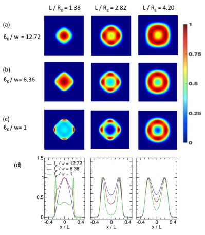
Figure 2: (a)–(c) Polymer COM probability distributions, ${\cal P}(x,y)$, for a system two hard-sphere chains confined to cavities with square cross sections of side length $L$. The cavities are scaled such that $h/R_{\text{g}}=0.282$ and the polymers each have a fixed number of Kuhn segments given by $\ell_{\text{c}}/\ell_{\text{k}}$=149. Each row corresponds to a different value of $\ell_{\rm k}/w$, and each column corresponds to a different scaled box width, $L/R_{\rm g}$. Distributions in rows (a) and (b) were calculated using semiflexible polymer chains, while those in row (c) used freely-jointed chains. (d) Cross sections of the distributions through $y=0$.

Figure 2 shows centre-of-mass (COM) probability distributions for either polymer in the $x-y$ plane, ${\cal P}(x,y)$. The distributions in row (a) show results for systems with a value of $\ell_{\rm k}/w$ that is approximately equal to the experimental value. Those in rows (b) and (c) have smaller values of $\ell_{\rm k}/w$. Since $\ell_{\rm c}/\ell_{\rm k}$ is fixed, these distributions in effect correspond to polymers of larger polymer width $w$. The distributions in row (c) were calculated using freely-jointed chains, as in our previous study.Polson and Rehel (2021) The distributions in each column correspond to three different values of $L/R_{\rm g}$. The graphs in row (d) are cross sections of the distributions for $y=0$. The distributions in the middle column were calculated for a box width of $L/R_{\rm g}$=2.82, which is approximately the value in the experiments. Thus, the columns on the left and right correspond to box widths smaller and larger than the experimental values, respectively. Note that the distribution calculated using conditions that best approximate those of the experiment of Capaldi et al.Capaldi et al. (2018) is that shown the middle panel of row (a).

Consider first the middle column, where $L/R_{\rm g}$=2.82. For all $\ell_{\rm k}/w$, the distributions show roughly the same qualitative features: a depletion zone in the middle of the box, and a ring-like structure containing four local high-probability spots located at the midpoints of the box edges. As noted in Ref. Polson and Rehel, 2021, entropic repulsion between the confined polymers tends to push them to opposite sides of the box. Thus, when the COM of one polymer is located at position $(x,y)$, the other tends to be at $(-x,-y)$, with the square box shape tending to favour positions at the box-edge midpoints. The depletion zone at the box centre results from the high entropic cost of polymer overlap for this box size. As $w$ increases, the packing fraction inside the cavity increases as well, increasing entropic repulsion between the chains and enhancing segregation. This appears as enhanced depletion in the box centre and an increased intensity of the probability ring. This is more clearly evident in the probability cross section graph in the middle panel of row (d). For the widest chains with $\ell_{\rm k}/w=1$, the polymer centre tends to further localize to four “hot spots”. Thus, high packing fraction promotes greater positional ordering in addition to segregation.

The effects of varying the cavity width are somewhat complicated. In the case of semiflexible chains ($\ell_{\rm k}/w=12.72$ and $\ell_{\rm k}/w=6.36$) there is a small enhancement in depletion at the box centre as the cavity width decreases from $L/R_{\rm g}=4.20$ to $L/R_{\rm g}$=2.82. This implies a slight increase in the degree of chain segregation. However, in decreasing the cavity width further to $L/R_{\rm g}=1.38$, lateral confinement overrides entropic repulsion, yielding distributions with polymer centers strongly localized in the middle of the cavity. Increasing chain thickness $w$ enhances chain repulsion, leading to a slight broadening of the central peak for $\ell_{\rm k}/w=6.36$ relative to that for $\ell_{\rm k}/w=12.72$. For the widest chains ($\ell_{\rm k}/w=1$) there is a similar enhancement in depletion at the box centre as $L$ decreases from $L/R_{\rm g}=4.20$ to $L/R_{\rm g}$=2.82, though the change is more pronounced than for semiflexible chains. Likewise, for the smallest cavities with $L/R_{\rm g}=1.38$ confinement overcomes the entropic repulsion, leading to an increase in the probability at the cavity center. In this extreme case of thick chains confined to a very small cavity, the combination of high packing fraction and lateral confinement yields a qualitatively distinct distribution with a broad central plateau with four high-probability peaks at positions comparable to those for the case of larger $L$.

To summarize, varying the polymer width and lateral confinement both strongly affect the equilibrium organization of the polymer chains. Generally, increasing chain width enhances entropic repulsion between chains and promotes segregation, while the effects of varying the degree of confinement are somewhat more complex. A partial depletion of DNA COM probability in the cavity centre was also observed in the experiments, consistent with the result for the system that best approximates the experimental conditions. Here, the observed ring-like structure is consistent with the interpretation of the dynamical behaviour of the $\lambda$ DNA molecules as collective Brownian rotation about the box centre. The sharp peaks observed for $\ell_{\rm k}/w$=1 and small boxes are spurious features produced by the unphysically high volume fraction for such polymer widths and are unlikely to be relevant to the systems studied in Ref. Capaldi et al., 2018. For the experimentally relevant box size ($L/R_{\rm g}=2.82$), using artificially wide polymer chains in simulations gives rise to features in ${\cal P}(x,y)$ that will likely impact the dynamics in simulations. Still, the gross features are sufficiently similar that the qualitative trends are expected to be similar except for the case of very small boxes.

IV.2 Asymmetry in polymer length

In this section we examine the physical behaviour of two confined polymers of different contour lengths. One motivation for considering such a system is provided by the experiments of Ref. Capaldi et al., 2018. In that study two confined $\lambda$-DNA strands were stained with different dyes (YOYO-1 and YOYO-3) in order to distinguish between them. Unlike the COM probability distributions presented in Sec. IV.1, there was a clear asymmetry in the experimental distributions. In particular, the DNA strand stained with YOYO-3 tended to lie closer to the centre of the box, while that stained with YOYO-1 was somewhat more displaced from the centre. This asymmetry most likely arises because the two dyes unwind the dsDNA by differing amounts, leading to slightly different contour lengths. In addition to that system, Capaldi et al. also examined a $\lambda$-DNA strand confined with a DNA plasmid, which has a much smaller contour length than $\lambda$-DNA. We anticipate that future experiments will extend this work and examine a larger number of contour length ratios. The simulation results presented in this section should be helpful for interpreting the results of such experiments. As before, we consider only confinement in a cavity with a square cross section, as in Ref. Capaldi et al., 2018.

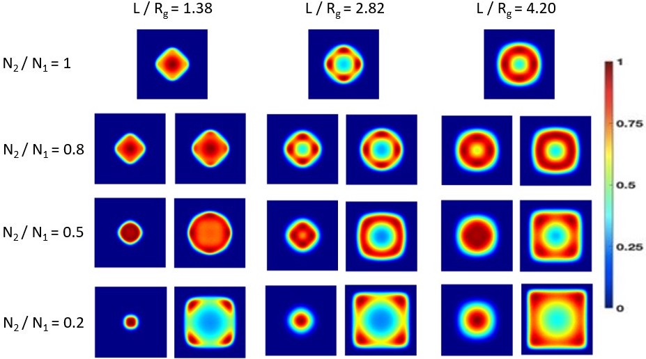
Figure 3: COM probability distributions, ${\cal P}(x,y)$, for a system of two semi-flexible hard-sphere chains of different lengths for various box widths and polymer-length aspect ratios. In these results $N_{1}=950$ and $N_{2}$ is variable. In addition, $h$=10.71 and $\ell_{\text{k}}=6.36$. The left-most graph in the pair of graphs in each column is the distribution for the longer polymer, while the right graph is that for the shorter polymer.

Figure 3 shows COM probability distributions ${\cal P}(x,y)$ for a system two semiflexible hard-sphere chains, one with length $N_{1}=950$ monomers and the second of variable length with $N_{2}\leq N_{1}$. Each chain has a Kuhn length of $\ell_{\text{k}}/w=6.36$. Results are shown for confinement to a box of height $h=10.71$ for three different values of the scaled cavity width, $L/R_{{\rm g}}$. For each case, the distributions for the two polymers become more dissimilar as the ratio $N_{2}/N_{1}$ decreases from unity, as the longer polymer tends to be more concentrated at the centre while the shorter one is pushed further from the centre. Notably, in cases of a large polymer length asymmetry, the shorter polymer tends to be pushed to the corners of the box. By contrast, for smaller length asymmetry, the centre-of-mass probability tend to be somewhat more focused at the midpoints of the sides of the box.

A theoretical calculation designed to reproduce all of the trends in Fig. 3 would be challenging and is beyond the scope of the present work. Here, we pursue instead the more modest goal of elucidating the behaviour in the case of large polymer length asymmetry (i.e. small $N_{2}/N_{1}$) and high packing fraction (i.e. low $L/R_{\rm g}$). We follow the approach taken in the recent study of Liu et al. in modeling the behaviour of a small plasmid in the presence a large DNA molecule in a nanoscale cavity.Liu et al. (2022) When the shorter polymer is sufficiently small, it is not expected to significantly perturb the monomer density of the larger polymer, $\rho_{\rm mon}(x,y)$. In this limit the interpolymer interaction free energy is approximately $F_{\rm int}=a\rho_{\rm mon}(x,y)$, where $(x,y)$ is the COM position of the small polymer and $a$ is a constant. [Note that the monomer density is defined to satisfy the normalization $\int_{\cal A}\rho_{\rm mon}(x,y)dxdy=N_{1}$, where the integral is over the area of the cross section.] The short polymer also interacts with the lateral walls with a free energy $F_{\rm wall}$ that depends on the distance to each wall. We used a simulation of a single confined polymer to directly calculate $\rho_{\rm mon}(x,y)$. In addition, we carried out a set of simulations to measure the variation of $F_{\rm wall}$ with COM distance from a single lateral wall using a multiple-histogram technique.Frenkel and Smit (2002) [See Appendix B of Ref. Polson and McLure, 2019 for details of a comparable calculation.]

Figure 4(a) shows the resulting probability distribution. The results are qualitatively consistent with the corresponding simulation result for the short polymer shown in Fig. 3 for $N_{2}/N_{1}=0.2$ and $L/R_{\rm g}=1.38$. The four probability peaks in the corners of the box are present. Figure 4(b) shows the monomer density for the larger polymer $\rho_{\rm mon}(x,y)$. Note the depletion zones near the edges of the box are enhanced near the corners, and it is this feature that tends to drive the smaller polymer into these locations. The interpolymer repulsion is counterbalanced by entropic repulsion of the small polymer with the walls. Figure 4(c) shows how the contributions of $F_{\rm int}$ and $F_{\rm wall}$, here measured as a function of displacement along the diagonal of the box, lead to the appearance of local free energy minima corresponding probability peaks in Fig. 4(a). As a result of the approximations employed the results are only qualitatively consistent with the simulation results. These calculations used a coupling value of $a/w^{2}=0.0236$, where $w$ is the polymer width and chosen unit of length (i.e., $w=1$). This value was chosen to yield the same ratio for ${\cal P}(x,y)$ at the peaks relative to that at the box centre ($x=y=0$) as in the simulation result in Fig. 3 for $N_{2}/N_{1}=0.2$ and $L/R_{\rm g}=1.38$.

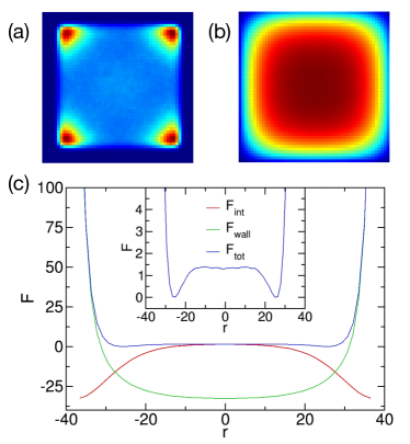
Figure 4: (a) Theoretical calculation for the COM distribution ${\cal P}(x,y)$ of the short polymer for a system with $L/R_{\rm g}=1.38$, $N_{2}/N_{1}=0.2$ and $N_{1}=950$. (b) Monomer density, $\rho_{\rm mon}(x,y)$ for a single polymer of length $N=950$ confined to the same box as in (a). (c) Variation of the free energy of the two-polymer system with distance along the diagonal of the box in the $x-y$ plane. $F_{\rm wall}$ is the free energy arising from interactions of the short polymer with the walls, $F_{1}$ is the interpolymer interaction free energy, and $F_{\rm tot}$ is the sum of the two. For convenience, $F_{\rm tot}$ has been vertically shifted so that $F_{\rm tot}=0$ at the minima. The inset shows a close-up of $F_{\rm tot}$.

The distributions in Fig. 3 can be characterized using the scaled RMS centre-of-mass displacement from the centre of the box, defined as

$$r_{i}^{*}\equiv\frac{\sqrt{\langle X_{i}^{2}+Y_{i}^{2}\rangle}}{L},$$ (7)

where $X_{i}$ and $Y_{i}$ are the COM coordinates of polymer $i$. The results are plotted in Fig. 5(a) for a system of two polymers confined to a box with a height of $h=$10.71 for various polymer length ratios and box sizes. In each case, $N_{1}=950$ and $\ell_{\text{k}}=6.36$. For each box size the shorter polymer is increasingly displaced from the centre of the cavity as $N_{2}/N_{1}$ decreases while the longer polymer is increasingly pushed toward the centre. This is consistent with the trends in Fig. 3. The inset in Fig. 5(a) shows the ratio $r_{2}^{*}/r_{1}^{*}$ vs the polymer length ratio. Note that $r_{2}^{*}/r_{1}^{*}$ is a measure of asymmetry in the probability distributions, with increasing asymmetry as $r_{2}^{*}/r_{1}^{*}$ increases from unity. Thus, the results show that the distribution asymmetry increases with increasing lateral confinement.

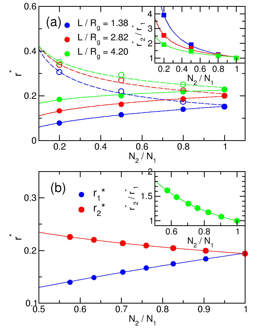
Figure 5: (a) Scaled RMS radial distance of each polymer from the centre of the box, $r_{1}^{*}$ (solid symbols) and $r_{2}^{*}$ (open symbols), vs the polymer length ratio, $N_{2}/N_{1}$. Results are shown for various box widths. The two chains each have a scaled Kuhn length of $\ell_{\text{k}}/w=6.36$, and the long polymer has a length of $N_{1}=950$. In all cases, the box height is $h$=10.71. The inset shows the ratio $r_{1}^{*}/r_{2}^{*}$ vs $N_{2}/N_{1}$. The solid and dashed lines are guides for the eye. (b) As in panel (a), except for fixed $N_{2}=1900$ and variable $N_{1}$. In addition, the Kuhn length is $\ell_{\text{k}}/w=12.72$, and the cavity dimensions are $h$=20 and $L$=200.

In the experiments of Refs. Capaldi et al., 2018 and Liu et al., 2022 Capaldi et al. examined the case of a small DNA plasmid confined with a much larger $\lambda$ DNA and observed that the plasmid was pushed out from the centre of the box while the larger one was more concentrated at its centre. This is qualitatively consistent with our results for small $N_{2}/N_{1}$. Unfortunately, their sampling was insufficient to determine if there was any preference for the plasmid to locate to regions near the corners of the box. They further noted an asymmetry in the distributions of two differently stained $\lambda$-DNA molecules, suggesting that the stains change the contour length of the molecules by different amounts. They speculated that the longer polymer is pushed to the edges as it would be more easily deformed. By contrast, our simulation data demonstrates it is instead the shorter polymer that tends to locate closer to the lateral walls.

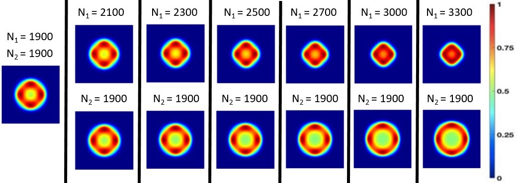
Figure 6: Probability distributions, ${\cal P}(x,y)$, for a system two semiflexible hard-sphere chains with $\ell_{\text{k}}=12.72$, $N_{\text{2}}$=1900 and various $N_{\text{1}}$. The polymers are confined to a box with a square cross section and dimensions of $L=200$ and $h=20$.

Staining DNA with dyes such as YOYO-1 has the effect of partially unwinding the double helix and increasing the contour length. While such effects have been well characterized for YOYO-1,Kundukad et al. (2014) those of YOYO-3 have been less studied. Quantifying the asymmetry between the two distributions presented in Ref. Capaldi et al., 2018 could in principle provide a means to estimate the contour length change caused by the latter dye. To explore this option we examined a two-polymer system in which one polymer has properties of $\lambda$ DNA stained with YOYO-1 under conditions corresponding roughly to those of the experiments of Ref. Capaldi et al., 2018. As in Sec. IV.1, we estimate that a YOYO-1 staining ratio of 10:1 (bp:fluorophore) increases the $\lambda$ DNA contour length by about 15% length from 16.5 $\mu$m to $\approx 19~{}\mu$m. Choosing an effective DNA width of $w=10~{}\mu$m, this corresponds to $\ell_{\rm c}/w=1900$. Consequently, we use a semiflexible polymer of length $N_{2}=1900$ monomers. In addition, we use a Kuhn length of $\ell_{\rm k}/w=12.72$. To model $\lambda$ DNA stained with YOYO-3, we assume this dye does not appreciably affect the Kuhn length or the effective width of the DNA, as is the case with YOYO-1.Kundukad et al. (2014) Since our simulation results suggest that DNA strands stained with YOYO-3 are longer than those stained with YOYO-1, we carry out a set of simulations for polymer lengths $N_{1}\geq N_{2}$. Finally, we use box dimensions of $L/w=200$ and $h/w=20$, which correspond to cavity the dimensions of $L=2$ $\mu$m and $h=200$ nm employed in Ref. Capaldi et al., 2018.

Figure 6 shows COM position probability distributions, ${\cal P}(x,y)$, for various values of $N_{1}$. As expected, the distribution for the longer polymer is more concentrated at the centre than is the case for the shorter polymer for all values of $N_{1}$. In addition, the distribution asymmetry grows with increasing polymer length asymmetry. Figure 5(b) shows the variation of $r_{1}^{*}$ and $r_{2}^{*}$ (defined in Eq. (7)) as well as the ratio, $r_{2}^{*}/r_{1}^{*}$, with respect to $N_{1}$. The results in Ref. Capaldi et al., 2018 were not presented in a manner to facilitate a straightforward comparison with the simulation results, and there may be insufficient spatial resolution to compare the distributions anyway. However, in principle it should be simple to calculate quantities like $r_{1}^{*}$ and $r_{2}^{*}$ from the experimental data. We anticipate that such analyses in future experimental studies in conjunction with these and future simulation results will provide a means to quantify the effect of YOYO-3 and other dyes on the physical properties of DNA.

IV.3 Anisometry in box geometry

Thus far, we have considered the behaviour of two polymers confined to a box-like cavity with a square cross section, in accord with the experiments of Ref. Capaldi et al., 2018. In a more recent study, Liu et al. Liu et al. (2022) examined the confinement in an elongated cavity with an elliptical shape in the lateral plane. As in Ref. Capaldi et al., 2018 they consider the case of two DNA strands of comparable length as well that of a long DNA strand confined with a much smaller plasmid. As in Ref. Capaldi et al., 2018, they examine the equilibrium organization and the dynamics of the confined molecules and show that both sets of properties are strongly affected by cavity elongation. Although other simulation studies have examined the effects of cavity elongation for similar two-polymer systems,Jun and Wright (2010); Jung et al. (2012b); Polson and Kerry (2018) to our knowledge, none have employed the type of confining geometry used in Ref. Liu et al., 2022, which is characterized by very strong confinement in one dimension between flat surfaces. The purpose of this section (as well as the following section) is to carry out simulations using a confining geometry that is relevant to such experiments. We first consider the simple case of two identical polymers confined to elongated cavities with a rectangular cross section and examine both the configurational statistics and the equilibrium dynamics. In the subsequent section we turn to cavities with elliptical cross sections and consider polymers of equal and unequal contour lengths.

As noted in our previous studyPolson and Rehel (2021) the simulations employed to study polymer dynamics are much less efficient than the MC simulations used to examine the configurational statistics. Consequently, systems using much shorter polymers are required in the former case for computational feasibility. As a key goal of the present work is to relate the equilibrium dynamics to the underlying free energy landscape of the system, the probability distributions for COM positions for such short-chain systems are needed. However, as noted for the case of cavities with square sections in Sec. IV.1 any attempt to model the experimental system with short freely-jointed chains leads to distributions that may differ significantly from those expected for the more realistic molecular models. Consequently, it is of value to first quantify this effect.

Figure 7 shows the effects of varying the polymer width on the COM distributions of two identical polymers confined to a box of lateral dimensions $L_{x}$ and $L_{y}(\geq L_{x})$. In each case, the cross-sectional area is fixed such that $\overline{L}/R_{\text{g},xy}=2.82$, where $\overline{L}\equiv\sqrt{L_{x}L_{y}}$ is the geometric mean lateral box length. In addition, we fix the ratios $h/R_{\text{g}}=0.282$, and $\ell_{\rm c}/\ell_{\text{k}}=149$, where $\ell_{\rm c}$ and $\ell_{\text{k}}$ is the contour length and Kuhn length, respectively. Results for three different values of $\ell_{\text{k}}/w$ are shown, each for three different cavity dimension asymmetries. Figures 7(a) and (b) show results for semiflexible chains of two different Kuhn lengths for model systems with properties comparable to those studied in the experiments. In each case, cavity elongation dramatically increases the tendency for the polymers to localize at two positions along the vertical dimension. The main qualitative effect of decreasing $\ell_{\rm k}/w$ is the enhancement of the depletion in the centre of the box, most notably for $L_{x}/L_{y}=0.8$. For the case of $\ell_{\rm k}/w=1$ in Fig. 7(c), this depletion is even more marked. In addition, the size of the two localized regions decreases. Similar results were noted in Sec. IV.1 for square cross sections. The results indicate that using an artificially large polymer width increases the tendency for the polymers to segregate.

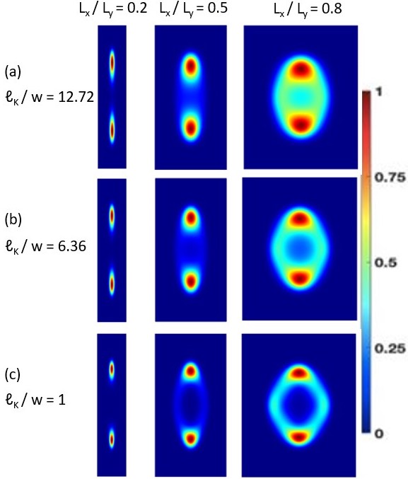
Figure 7: Probability distributions for a system two semiflexible hard-sphere chains with various widths confined to cavities with rectangular cross sections. The cavity dimensions satisfy $\overline{L}/R_{\text{g},xy}=2.82$, $\bar{L}/h=10$. For all $\ell_{\text{k}}/w$ values, the contour length is fixed to $\ell_{\rm c}/\ell_{\text{k}}=149$.

Figure 8 shows centre-of-mass position probability distributions in the lateral plane for two freely-jointed LJ chains, each of length $N$=60, confined to a cavity a box height of $h=4$. Note that the LJ chain model is also amenable for use in dynamics simulations, which are indeed used later in this section to characterize the equilibrium dynamics for chains of this length. Results are shown for several values of the geometric mean box width, $\overline{L}$, as well as for various values of $L_{x}/L_{y}$. The trends for varying $L_{x}/L_{y}$ are qualitatively similar to those of Fig. 7, which were calculated for hard-sphere chains. As the box becomes more elongated, i.e., as $L_{x}/L_{y}$ decreases, the polymers tend to segregate along the long axis of the box for all box sizes. The exception is for $\overline{L}/R_{{\rm g},xy}=13.66$, where the box is so large the polymers only rarely interact with each other.

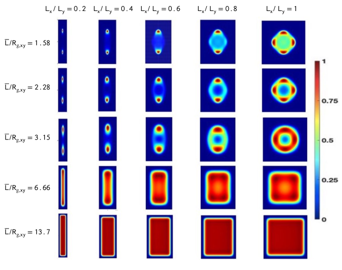
Figure 8: COM probability distributions for a system two fully flexible LJ chains of length $N$=60 confined to a box of height $h$=4 and a rectangular cross sections. Results are shown for various values of the scaled cavity width, $\overline{L}/R_{{\rm g},xy}$, and box aspect ratio, $L_{x}/L_{y}$.

To better characterize the effects of cavity anisometry on these distributions, we employ two different measures of the centre-of-mass displacement from the box centre, located at $(x,y)=(0,0)$, each in both the $x$ and $y$ directions. The first is defined

$$\xi_{x}\equiv\sqrt{\langle X^{2}\rangle/\langle X_{\rm sq}^{2}\rangle},$$ (8)

where $X$ is the centre-of-mass position of either polymer in the $x$-direction. In addition, $X_{\rm sq}$ is the COM position for a box with a square cross section, where $L_{x}/L_{y}=1$. The quantity $\xi_{y}$ is likewise defined for the $y$ direction. The second measure is defined

$$X^{*}\equiv{\sqrt{\langle X^{2}\rangle}}/{\overline{L}}.$$ (9)

The quantity $Y^{*}$ is similarly defined for the $y$-direction.

Figure 9(a) shows $\xi_{x}$ and $\xi_{y}$ vs $L_{x}/L_{y}$ for various box sizes. As the box elongates (i.e., $L_{x}/L_{y}$ decreases from unity), $\xi_{x}$ decreases, indicating that the distributions narrow along the $x$ direction, i.e. along the short lateral dimension. This effect is enhanced by reducing the box size, i.e., the rate of decrease in $\xi_{x}$ from unity is greater as $\overline{L}$ decreases because the depletion layer near the walls takes up a greater fraction of the box width along $x$. By contrast, $\xi_{y}$ increases, indicating that the polymers are each displaced farther away from the box centre in the $y$-direction, consistent with the increased tendency for polymer segregation along this axis and the increasing distance between probability peaks in Fig. 8. This effect is enhanced by reducing the box size, i.e., the increase of $\xi_{y}$ from unity is greater as $\overline{L}$ decreases. For such smaller boxes, the polymers are forced into contact with each other, and the only means to prevent overlap is for each to avoid the box centre.

Figure 9(b) shows the variation of $X^{*}(=Y^{*})$ with box size for the case of square cavities with $L_{x}/L_{y}=1$. The decrease of $X^{*}$ with $\overline{L}/R_{{\rm g},xy}$ is due to the increasing fraction of the box interior occupied by the entropic depletion zones near the walls and corners as the cavity size is reduced. This effect inhibits the polymers from moving too far from the centre. Finally, Fig. 9(c) shows the variation of the ratio $Y^{*}/X^{*}$ ($=\langle Y^{2}\rangle/\langle X^{2}\rangle$) with box anisometry, $L_{x}/L_{y}$. This ratio increases with decreasing $L_{x}/L_{y}$ faster for the smaller boxes. These measures of polymer position and organization provide a simple means for quantitative characterization of the 2D probability distributions in Fig. 8 that should be beneficial for comparison of results with those of future nanofluidics experiments employing rectangular cavities.

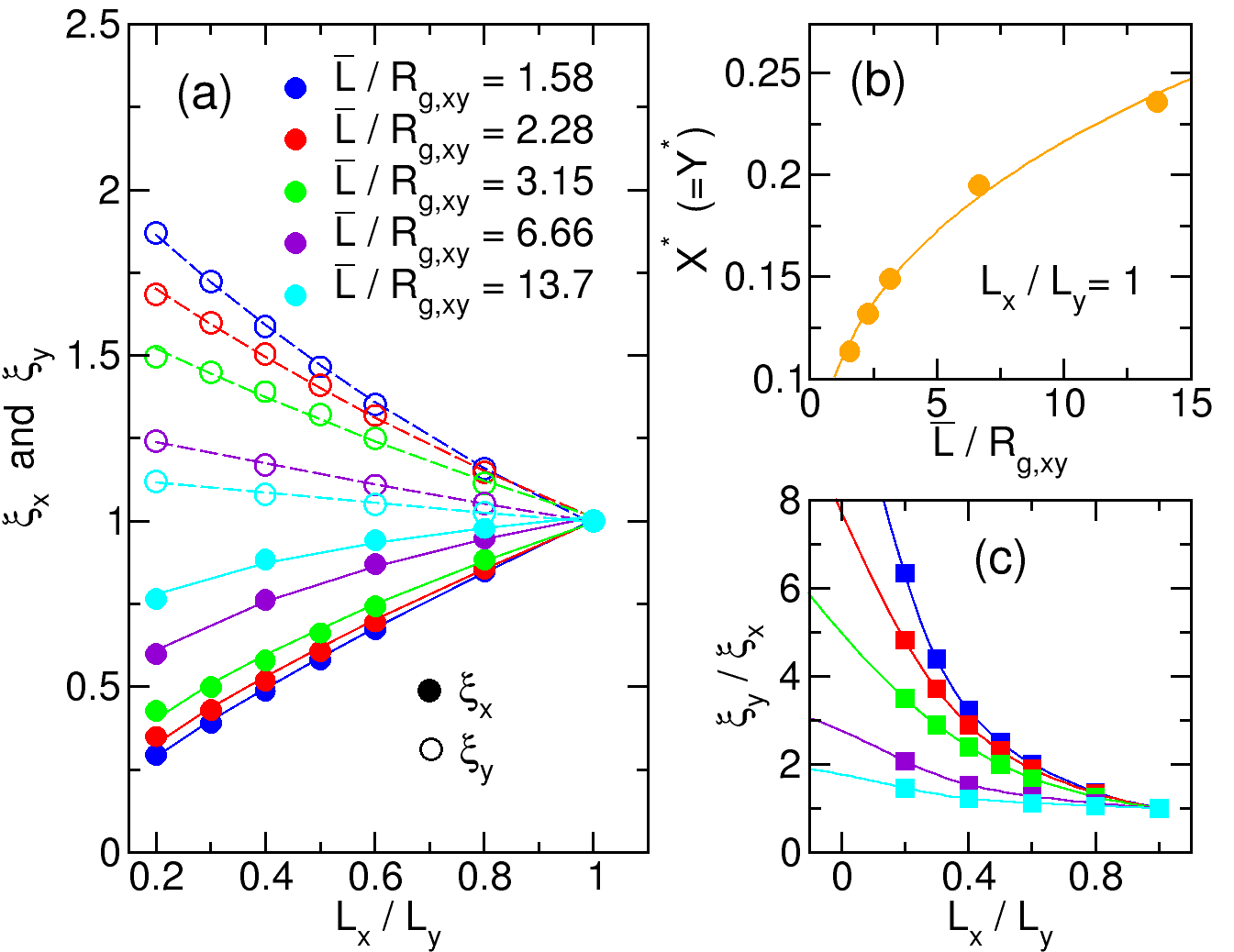
Figure 9: (a) Variation of $\xi_{x}$ and $\xi_{y}$ (defined in Eq. (8)) with box anisometry, $L_{x}/L_{y}$. Results are shown for various box sizes for a system of two fully-flexible LJ chains with $N$=60 confined to a box of height $h=4$. (b) Variation of $X^{*}$ ($=Y^{*}$) (defined in Eq. (9)) with scaled box size for square boxes. (c) Ratio $\xi_{x}/\xi_{y}$ vs box anisometry using the results shown in panel (a).

Let us now consider the equilibrium dynamics of polymers confined to an anisometric box. Figure 10 shows two sample histories of the COM coordinate $Y$ for systems with polymers of length $N=60$ in cavities of different size and shape. Note that the centres of mass tend to be localized at positions at opposite ends of the elongated box, corresponding to the two high probability local regions in the ${\cal P}(x,y)$ distributions for elongated boxes ($L_{x}/L_{y}<1$) in Fig. 8. The histories also show that the polymers occasionally swap positions. The distributions of Fig. 8 suggest that these swapping events will occur along a pathway that depends strongly on $L_{x}/L_{y}$. In the limit of large $L_{x}/L_{y}$, the polymers partially segregate along the $x$ axis as their centres cross the $y=0$ boundary. By contrast, for more elongated boxes with small $L_{x}/L_{y}$, no such segregation along the $x$ dimension is observed, and the COM of each polymer passes through the centre of the box during a chain swapping event. In this case, much greater interpenetration of the chains occurs during the free energy barrier crossing.

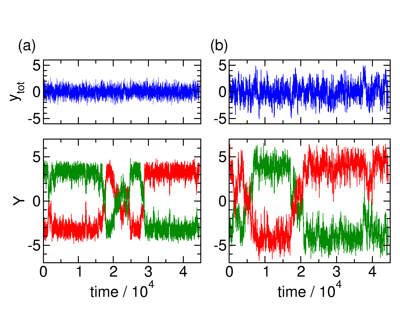
Figure 10: Position histories for a system of two fully flexible LJ chains where $N$=60. (a) The top graph shows the history of combined COM of both polymers, $y_{\text{tot}}=Y_{1}+Y_{2}$, while the bottom graph shows the history of the coordinate of each polymer. The rectangular cavity dimensions are such that $L_{x}/L_{y}=0.4$ and $\overline{L}/R_{{\rm g},xy}=1.58$. (b) As in (a), except for $L_{x}/L_{y}=0.5$ and $\overline{L}/R_{{\rm g},xy}=2.28$.

Let us consider the case of an elongated box with $L_{x}/L_{y}\lesssim 0.6$, where the the position swapping occurs via the latter mechanism described above. We define the dwell time $t_{\rm d}$ as the as the time between consecutive crossings of the $y$=0 boundary separating the two halves of the box. The distribution of the dwell times for two different box asymmetries is shown in Fig. 11. In each case, the distribution is exponential at long times with a notable deviation at very short times. The short-time probability peak arises from rapid small-amplitude back-and-forth fluctuations as each polymer passes through the box centre at a local free-energy maximum. A similar feature was also noted in the experiments of Ref. Liu et al., 2022.

The exponential form of the dwell-time distributions can be understood using a simple model. First, note that polymer centres of mass tend to be strongly anti-correlated along the $y$ axis, in the sense that if one polymer COM has a coordinate $y$, the other tends to have a coordinate of $-y$. Increasing the box elongation tends to enhance this effect. Assuming (1) perfect anticorrelation between the COM positions of the polymers, (2) highly localized centre-of-mass positions, and (3) that the time spent transitioning between states is negligible, the problem of tracking the dynamical behaviour of two polymers reduces to that of a single polymer that rapidly jumps between two possible centre-of-mass positions. This is just a simple two-state dynamical model. It is well known that the probability distribution for the time spent in either state between successive jumps, $t_{\text{d}}$, for such a two-state model described by a transition rate $k_{0}$ is given byPhillips et al. (2012)

$$\mathcal{P}(t_{\text{d}})\propto\exp\left(-t_{\text{d}}/\tau_{\rm d}\right),$$ (10)

where the decay constant $\tau_{\rm d}$ is given by $\tau_{\rm d}=k_{0}^{-1}$. This simple two-state model therefore accounts for the exponential decay of the distributions shown in Fig. 11.

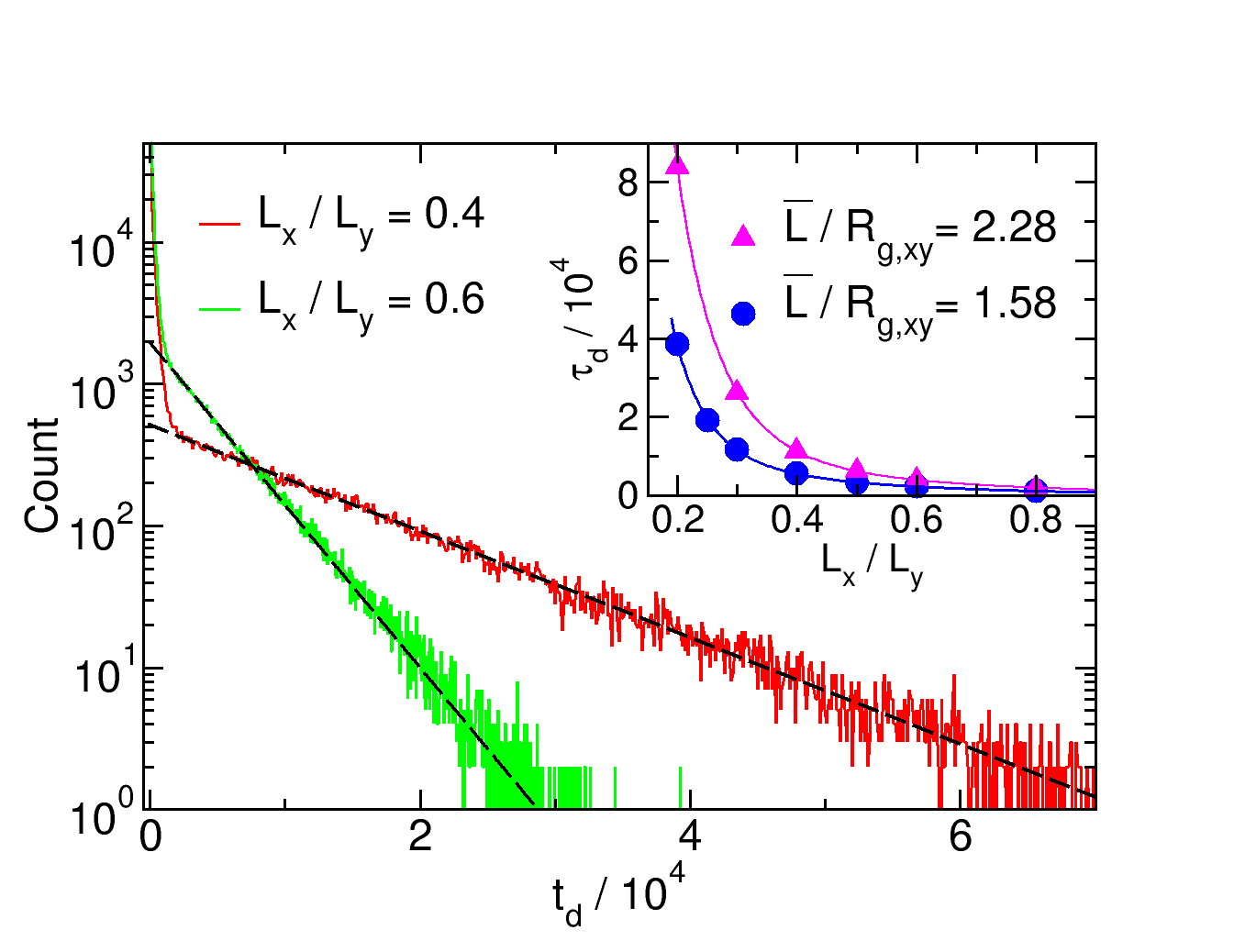
Figure 11: Count distribution for the dwell times for a system with $N$=60 and $\overline{L}/R_{{\rm g},xy}=2.28$. Results are shown for $L_{x}/L_{y}$=0.4 and $L_{x}/L_{y}$=0.6 for the red and green curves, respectively. The dotted lines are fits to a exponential of the form $\exp(-t_{\rm d}/\tau_{\rm d})$ with time constants of $\tau_{\rm d}=(1.16\pm 0.01)\times 10^{4}$ for $L_{x}/L_{y}=4$ and $\tau_{\rm d}=(3.79\pm 0.03)\times 10^{3}$ for $L_{x}/L_{y}$=0.6. The inset shows the variation of $\tau_{\rm d}$ with $L_{x}/L_{y}$ for two different scaled cavity sizes.

The values of the time constant $\tau_{\rm d}$ can easily be obtained by a fit to the measured dwell time distributions. Sample fits are shown as dashed lines in Fig. 11. Note that we exclude the spurious peaks at small dwell times from the fits. The inset shows the variation of the time constant with respect to $L_{x}/L_{y}$ for two different values of the scaled lateral box size, $\overline{L}/R_{{\rm g},xy}$. Generally, for fixed cross-sectional area, $\tau_{\rm d}$ increases monotonically with increasing cavity elongation (i.e., decreasing $L_{x}/L_{y}$ from unity). The results are qualitatively consistent with comparable experimental results for elliptical cavities (see Fig. 3(d) of Ref. Liu et al., 2022). The effect is diminished by reducing the lateral cavity size, $\overline{L}/R_{{\rm g},xy}$.

The value of the time constant is largely determined by the features of the probability distributions in Fig. 8. This relationship can be elucidated using a multidimensional generalization of Kramers theory,Matkowsky et al. (1988) which predicts

$$e^{\Delta F/k_{\rm B}T}=D\tau_{\text{d}}^{*},$$ (11)

where

$$\tau_{\rm d}^{*}\equiv\frac{Q_{\text{B}}\omega_{\text{B}}\omega_{\text{W}}}{2\pi Q_{\text{W}}}\tau_{\rm d}.$$ (12)

Here, $D$ is the Rouse diffusion coefficient, $\Delta F$ is the free energy barrier height, and $\omega_{\text{B}}$ and $\omega_{\text{W}}$ represent the effective frequencies of the well and barrier, respectively. In addition, $Q_{\text{B}}$ and $Q_{\text{W}}$ are the partition functions associated with the non-reactive modes at the free energy barrier and well, respectively. The details for the procedure used to extract $\omega_{\text{B}}$, $\omega_{\text{W}}$, $Q_{\text{B}}$ and $Q_{\text{W}}$ from the free energy landscape are given in Section I of the ESI.†

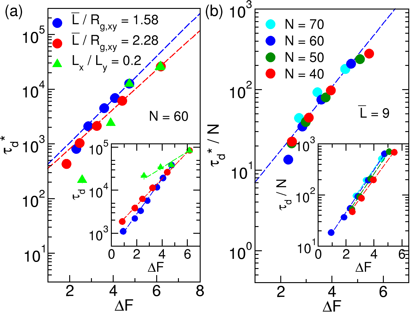
Figure 12: (a) Scaled time constant, $\tau_{\rm d}^{*}$ (defined in Eq. (11)) vs the free energy barrier height. Circles indicate changing $\Delta F$ by varying $L_{x}/L_{y}$ for fixed $N$ and $\overline{L}$, and triangles indicate changing $\Delta F$ by varying $\overline{L}$ and fixing $L_{x}/L_{y}$ and $N$. The curves are fit to exponential functions, $\tau_{\rm d}^{*}\propto e^{\alpha\Delta F}$, with $\alpha=0.90\pm 0.03$ for $\overline{L}/R_{{\rm g},xy}=1.58$ and $\alpha=0.83\pm 0.02$ for $\overline{L}/R_{{\rm g},xy}=2.28$. The inset shows the unscaled time constant vs the barrier height. The dashed curves are fits to exponential functions. (b) $\tau_{\rm d}^{*}/N$ vs $\Delta F$ for several values of $N$ and for $\overline{L}=9$. The curves are fit to the exponential function, $\tau_{\rm d}^{*}/N\propto e^{\alpha\Delta F}$, with $\alpha$=0.90. The inset shows $\tau_{\rm d}/N$ vs $\Delta F$. The dashed lines are fits to exponential functions.

Figure 12(a) shows the variation of $\tau_{\rm d}^{*}$ with $\Delta F$. Two data sets correspond to fixed box cross-sectional area, one with $\overline{L}/R_{{\rm g},xy}=1.58$ and the other with $\overline{L}/R_{{\rm g},xy}=2.28$. In each case, $\Delta F$ is controlled by variation in the box anisometry, $L_{x}/L_{y}$, with larger anisometries leading to higher barriers. With the exception of the systems with very low $\Delta F$, where the Kramers theory is not expected to hold, $\tau_{\rm d}^{*}$ increases exponentially with $\Delta F$, in agreement with the theoretical prediction of Eq. (11). The curves were fit to exponential functions of the form $\tau_{\text{d}}^{*}=C\exp(\alpha\Delta F)$. In the case of $\overline{L}/R_{{\rm g},xy}=1.58$ we find $\alpha\approx 0.90\pm 0.03$, agreeing reasonably well with the predicted value of $\alpha=1$. However in the larger box size of $\overline{L}/R_{{\rm g},xy}=2.28$ we find $\alpha=0.83\pm 0.02$, which deviates a little more from the predicted value. In the remaining data set, the anisometry is held fixed at $L_{x}/L_{y}=0.2$ and $\Delta F$ is controlled by varying the cross-sectional area. Here, $\tau_{d}^{*}$ does not appear to vary exponentially with $\Delta F$. Figure 12(b) shows the variation of $\tau_{\rm d}^{*}/N$ with $L_{x}/L_{y}$ for fixed $\overline{L}$ for several values of $N$. Since the Rouse diffusion coefficient in Eq. (11) scales as $D\propto 1/N$, the model predicts $\tau_{d}^{*}/N$ to be invariant with respect to $N$. The data collapse onto a single curve is consistent with this prediction. The curve is approximately exponential and characterized by $\alpha=0.9$, close to the value of $\alpha=1$ predicted by the model.

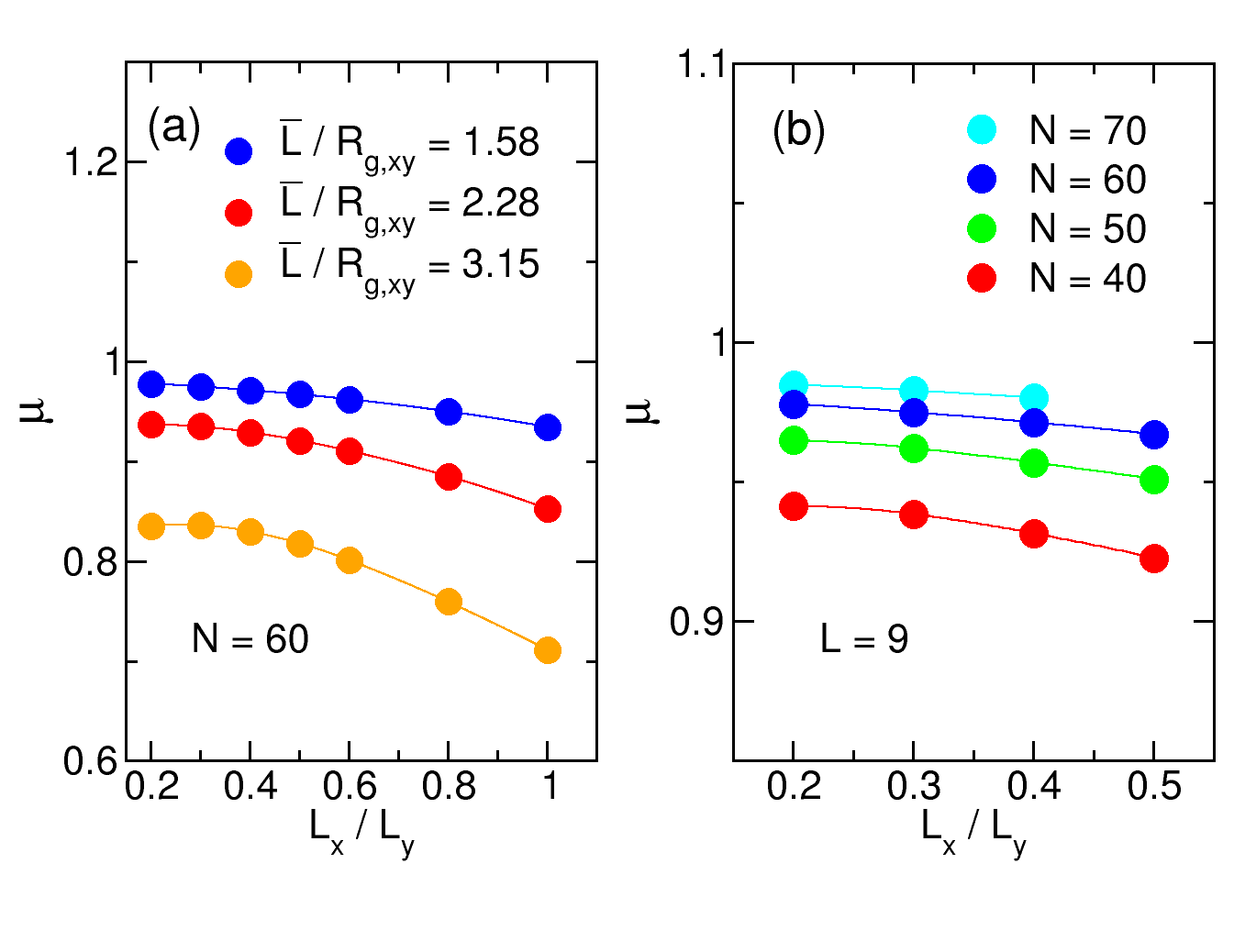
Figure 13: COM position anticorrelation, $\mu$, for a system of two fully flexible LJ polymers vs $L_{x}/L_{y}$ (a) for $N=60$ and several values of $\overline{L}/R_{{\rm g},xy}$, and (b) for $\overline{L}/R_{{\rm g},xy}=1.58$ and several values of $N$.

As noted earlier, the theoretical model used to analyze the scaling of the dwell time constant assumes perfect anticorrelation in the positions of the two polymers. The small deviation between the observed and predicted scaling behaviour could arise in part from a breakdown in this assumption. To investigate this possibility, we measure the degree of anticorrelation, $\mu$, between the COM $y$-coordinates of the two polymers, defined as

$$\mu=-\frac{\langle Y_{\text{1}}Y_{\text{2}}\rangle}{\langle Y^{2}\rangle},$$ (13)

where $\langle Y^{2}\rangle\equiv\langle Y_{1}^{2}\rangle=\langle Y_{2}^{2}\rangle$.

Fig. 13(a) shows the variation of $\mu$ with the box anisometry, $L_{x}/L_{y}$, for three values of the scaled box size, $\overline{L}/R_{{\rm g},xy}$ for a chain length of $N=60$. The data correspond to those in Fig. 12(a). Two trends are apparent. First, position anticorrelation increases with decreasing box size. The data for the smallest box size of $\overline{L}/R_{{\rm g},xy}=1.58$ are closest to the value of $\mu=1$ assumed in the two-state model. In addition, for each cavity size, there is a small decrease in the position anticorrelation with decreasing cavity elongation (i.e., as $L_{x}/L_{y}$ increases), with more a rapid decrease for the larger boxes. The decrease in anticorrelation as both $\overline{L}$ and $L_{x}/L_{y}$ increase also correlates with the relative size of the fluctuations of $y_{\text{tot}}=Y_{1}+Y_{2}$ in Fig. 10. This arises from the fact that as $L_{x}/L_{y}$ decreases from unity the two probability peaks become more sharply localized at the positions on opposite sides of the cavity. We speculate that the decrease in $\mu$ with $\overline{L}/R_{{\rm g},xy}$ is a primary cause for why the measured value of $\alpha$ obtained from fits to the data in Fig. 12(a) decrease below the ideal value of unity with increasing $\overline{L}/R_{{\rm g},xy}$. It also likely accounts for the non-exponential behaviour in Fig. 12(a) for the data set with fixed $L_{x}/L_{y}=0.2$ obtained by varying $\overline{L}/R_{{\rm g},xy}$. Figure 13(b) shows that the anticorrelation increases only slightly as the polymer length $N$ increases. Thus, varying $N$ over the range considered here is not expected to significantly affect the calculated value of $\alpha$, consistent with the data collapse observed in Fig. 12(b).

The effects of varying the cavity volume and elongation on the organization and dynamics of the polymers are qualitatively consistent with trends predicted by Jun and Wright using the blob model for a comparable physical system.Jun and Wright (2010) In sufficiently elongated cavities, the blob size is comparable to the cavity width, and the strong repulsion between the blobs ensures linear ordering along the cavity and, thus, chain segregation. For less elongated cavities of the same volume, the blob size shrinks in size relative to the cavity width, and inter-blob repulsion no longer enforces linear ordering. Instead, the string of blobs for each chain effectively undergoes a self-avoiding walk, resulting in a mixed state in which the chains no longer segregate. These predictions were corroborated by simulations.Jung et al. (2012b, a) The increase in chain miscibility with decreasing cavity elongation is accompanied by a decrease in the free-energy barrier separating the most probable polymer centre-of-mass positions along the cavity, an effect quantified in Ref. Polson and Kerry, 2018. In both the theory and in these previous simulations, miscibility is enhanced by decreasing the cavity volume. All of these trends are consistent with those evident in the probability maps of Fig. 7 and 8, and so account for the trends in the chain-swapping dynamics in Figs. 9, 10, 11, and 12. One feature of the present system that complicates direct comparison with the predictions of Ref. Jun and Wright, 2010 is the particularly small cavity dimension in the longitudinal direction ($h$), so chosen to mimic the experimental systems. This leads to confinement with three different dimensions for the elongated rectangular cavities, in contrast to the case in Ref. Jun and Wright, 2010, where two cavity dimensions were equal. In addition, the small system sizes employed here are likely too small for the blob model to yield quantitatively accurate results. It is intriguing that the qualitative trends of the predictions nevertheless hold up. Further investigation using much larger system sizes and varying $h$ the would be of value in assessing the applicability of the theory to this system.

To summarize, increasing cavity elongation in the lateral plane tends to promote segregation, an effect that is enhanced by decreasing the lateral cavity size. A concomitant increase in the free energy barrier between two localized positions leads to a reduction in the rate of swapping. For sufficiently small cross-sectional area and large cavity anisometry, the process is reasonably well described using a two-state model together with a multi-dimensional extension of Kramers theory for activated processes. The observed small discrepancies arise from the marginal validity of some of the approximations, notably the breakdown in the assumption of perfect position anticorrelation of the two polymers. The results presented here are in broad agreement with those of the recent experimental study of Ref. Liu et al., 2022. Note that the dynamics simulations employed short ($N=60$ monomers) freely-jointed polymer chains due to the time-consuming nature of the calculations. While this produces artificially wide polymers in relation to the $\lambda$ DNA chains used in the experiments the scaling analysis of Fig. 7 suggest comparable behaviour for realistic values of chain thickness $w$.

IV.4 Elliptical cavities

The recent study by Liu et al.Liu et al. (2022) examined the behaviour of two DNA molecules confined to a cavity with an elliptical cross section in the lateral plane. They studied the configurational statistics and dynamics of two different systems, one with two $\lambda$-DNA molecules and another consisting of a T₄-DNA molecule and a single plasmid vector. Although the two $\lambda$ DNA molecules have slightly different contour lengths due to the use of different dyes, as noted earlier, they are of comparable magnitude. On the other hand, the T₄-DNA molecule (166 kbp) is considerably longer than the plasmid (4361 bp) and has a different topology (i.e. linear vs ring). Not surprisingly, the two systems exhibit qualitatively different behaviour. In this section, we carry out simulations for models that roughly correspond to these different systems in order to better understand the trends observed in the experiments. Note that the latter system exhibits asymmetries in both confinement cavity dimensions and polymer length.

In the first system, we use two identical semiflexible polymers, each of length $N=1900$ monomers and bending rigidity $\kappa=6.36$. These values lead to lengthscale ratios $\ell_{\rm c}/w$ and $P/w$ that correspond roughly to two $\lambda$-DNA molecules stained with YOYO-1 under typical experimental conditions. We use a cavity height of $h=20$ and a cross-sectional area of $A=40000$, corresponding to a ratio of $\bar{L}/R_{{\rm g},xy}=2.6$, where $\bar{L}\equiv\sqrt{A}$ and the value of $R_{{\rm g},xy}$ is calculated for a slit of height $h=20$. Figure 14 shows COM probability distributions, ${\cal P}(x,y)$, for confining cavities with eccentricities of $e=0.3$, $0.6$ and $0.9$. The graphs on the right side of the figure show probability cross sections through the vertical ($y$) and horizontal ($x$) symmetry axes of the ellipses. The qualitative trends are similar to those observed for rectangular boxes in Figs. 7 and 8. The key trend is an increased tendency for the polymers to occupy two localized positions as the eccentricity increases, i.e., as the box becomes more elongated. For a highly elongated cavity with $e=0.9$, we note two quasi-discrete areas of high probability along the long axis of the box, indicating the polymers segregate along the long axis. In this limit, the polymers are expected to undergo the same activated dynamics described in the previous section. In the case of a low degree of cavity elongation for $e=0.3$, the distribution has a ring-like structure with slight enhancements along the long axis of the box. This indicates that the polymers segregate; however, there is only a slight orientational preference due to the nearly circular shape of the cavity. In this regime, the polymers are expected to undergo Brownian rotation. In between these extremes at $e=0.6$, the distribution is somewhat more complex. There is a faint probability ring as for more circular boxes, though the orientational preference is still relatively strong compared to $e$=0.3. These results are qualitatively consistent with those for two $\lambda$-DNA molecules confined to an elliptical cavity reported in Ref. Liu et al., 2022.

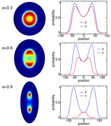
Figure 14: COM probability distributions for a system of two semiflexible hard-sphere chains, each of length $N=1900$ and bending rigidity $\kappa=6.36$, confined to a cavity of height $h=20$ with an elliptical cross section of area $A=40000$. The left column shows 2D distributions, ${\cal P}(x,y)$, for eccentricities of $e=0.3$, $0.6$ and $0.9$. The graphs in the right column show the corresponding cross sections of the distributions along the vertical ($y$) and horizontal ($x$) symmetry axes of the distributions.

Next, we consider a two-polymer system consisting of a large linear polymer and a short ring polymer. The long polymer is chosen to have a length of $N_{1}=1000$ monomers and a bending rigidity of $\kappa=6.36$, while the ring polymer has a length of $N_{2}=25$. Note that the contour-length ratio is comparable to that of the T₄/plasmid system studied in Ref. Liu et al., 2022. We choose a box with an elliptical cross section of area $A=3000$ and a height of $h=15$. This corresponds to $\bar{L}/R_{{\rm g},xy}=0.94$, where $R_{{\rm g},xy}$ is the lateral rms radius of gyration of the long polymer confined to a slit of $h=15$. This is a very high degree of lateral confinement. Figure 15(a)–(c) shows probability distributions of the ring polymer for cavity eccentricities of $e=0$, $0.8$ and $0.95$. In all cases there is an enhanced probability for the ring polymer to lie near the lateral wall of the cavity. The origin of this trend is straightforward. This region corresponds to an entropic depletion zone for the large polymer, and the short polymer is naturally drawn into it to avoid collisions with the other polymer and thus increase its own conformational entropy. As the cavity becomes more elongated, the short polymer increasingly favours the regions near the poles of the ellipse over regions near the less curved parts of the wall. These trends are also evident in the graphs in Figs. 15(g)–(i), which show cross sections of the distributions along the symmetry axes of the ellipses. The overall trends are in qualitative agreement with the experimental results of Ref. Liu et al., 2022. Note that the ring topology of the short polymer has only a minor effect on its position probability distribution. As evident in the results presented in section II of the ESI†, employing linear topology for the short polymer increases only slightly the entropic repulsion of the lateral confining walls, a consequence of the somewhat larger average size of the linear polymer.

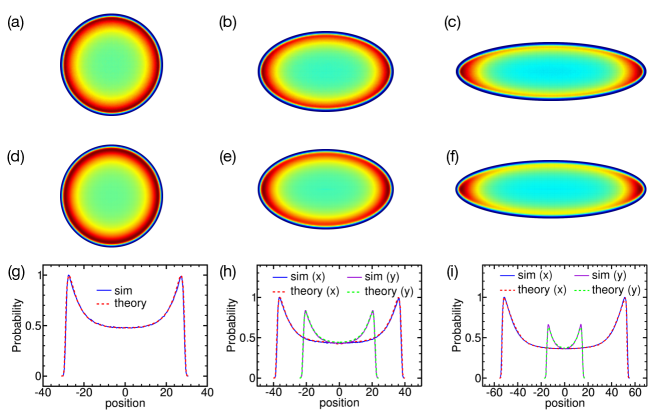
Figure 15: COM probability, ${\cal P}(x,y)$, for a ring polymer confined with a large linear polymer in a cavity with elliptical cross section. The cavity has a cross-sectional area of $A=3000$ and a height of $h=15$. The ring polymer has a length of $N_{2}=25$, and the linear polymer has a length of $N_{1}=1000$ and a bending rigidity of $\kappa=6.36$. Panels (a), (b) and (c) show simulation results for cavities with eccentricity $e=0$, $0.8$ and $0.95$, respectively. Panels (d), (e) and (f) show corresponding results from a theoretical model for the distributions in the top row. The graphs in (g), (h) and (i) show cross sections of the distributions along the horizontal ($x$) and vertical ($y$) symmetry axes of the distributions.

To better understand the observed bahaviour, we employ a theoretical model used in Ref. Liu et al., 2022, which was also used earlier in Section IV.2, to understand polymer organization for polymers of very different lengths confined to a square box (see Fig. 4). As before, we construct a 2D free-energy function for the centre of mass of the short (i.e., ring) polymer that is a sum of two contributions, $F(x,y)=F_{\rm int}(x,y)+F_{\rm wall}(x,y)$. The interaction free energy with the large polymer is chosen to have the form $F_{\rm int}(x,y)=a\rho_{\rm mon}(x,y)$, where $\rho_{\rm mon}(x,y)$ is the monomer density of the large polymer, which is assumed to be unperturbed by the presence of the short one. In addition, $F_{\rm wall}(x,y)$ is the free energy associated with the interaction of the ring polymer with the lateral wall, which is only appreciable when that polymer is very close to the wall. We calculate $\rho_{\rm mon}(x,y)$ from a separate simulation with only the linear polymer present. In addition, we calculate $F_{\rm wall}(x,y)$ using a multiple-histogram MC simulation for a ring polymer of length $N_{2}=25$ confined to a slit of height $h=15$ and in the vicinity of a single hard flat wall in the lateral dimension. We find that the variation of $F_{\rm wall}$ with the COM distance from the wall is well approximated by an exponential of the form $F_{\rm wall}(r)=b\exp(-r/r_{b})$, where $b=25.12$ and $r_{b}=1.60$. Calculation of the resulting probability distribution, ${\cal P}(x,y)\propto\exp(-F(x,y)/k_{\rm B}T)$ yields the results shown in panels (d), (e) and (f) of Fig. 15 using values of $a/w^{2}=0.650$, 0.634 and 0.658 for $e=0.95$, $e=0.95$, and $e=0$, respectively. The calculated distributions match the corresponding simulation results very closely. A clearer comparison is provided by the graphs shown in Figs. 15(g)–(i), in which cross sections of the calculated probability along the distribution symmetry axes are overlaid on those obtained directly from the simulation. These results are unambiguous: the theoretical model provides an exceptionally good prediction of the organization of the short ring polymer in the presence of a much longer linear polymer confined to the elliptical cavity at sufficiently high density.

To assess the measured values of the coefficient, $a$, we follow the procedure in Ref. Liu et al., 2022. The repulsive term in the Flory free energyde Gennes (1979) is given by $k_{\rm B}Tv_{\rm ex}\rho$, where $v_{\rm ex}$ is the excluded volume and $\rho$ is the Kuhn segment concentration. Using the values of $\ell_{\rm k}$ and box height $h$ we convert $\rho$ to the the 2D monomer density, $\rho_{\rm mon}$. Next, we equate the repulsive Flory free energy term to $F_{\rm int}=a\rho_{\rm mon}$ using a value of $a=0.65$ in order to calculate the effective excluded volume of the ring polymer. Approximating this as a sphere of radius $r_{\rm p}$, we find that $r_{\rm p}\approx 3.1$, which is close to the measured bulk RMS radius of gyration of the ring polymer of $R_{\rm g}=2.31$. We conclude that the model for the interaction between the short ring polymer and the linear polymer yields physically meaningful values of $a$.

In their analysis of the data for T₄-DNA/plasmid confinement in elliptical cavities, Liu et al. found generally good agreement with the probability density cross sections. However, statistical scatter of the data precluded a test of the model as quantitative as is provided in the present study. Their analysis also involved estimation of the linear-polymer density profile by numerical solution of a partial differential equation and invoking ground-state dominance. The authors note that the calculated distribution is expected to become inaccurate near the poles as the cavity becomes increasingly elongated. This is a regime where the semiflexiblity of the polymer is expected to become significant, a feature which was not incorporated into the calculation. The analysis of the simulations show that modeling the interpolymer interactions with a free energy $F_{\rm int}\propto\rho_{\rm mon}(x,y)$ can indeed be a decent approximation in the case where excluded-volume interactions dominate and provided the polymer size ratio is sufficiently large. This should be useful information for analysis of comparable data in future experiments.

Of final note is the contrast in the quality of the theoretical predictions for the elliptical cavities here and the square cavities in Sec. IV.2 (see Fig. 4). While the predicted distributions in the latter case are qualitatively correct, the quantitative discrepancies with the simulation data were significant. This is mostly due to the larger size of the short polymer in that case, where the contour-length ratio was 5:1. By contrast, the size ratio here is close to 40:1, and the ring topology of the small polymer contributes to making it even more compact. Both factors reduce the degree to which the short polymer perturbs the configuration of the larger one, which is an underlying assumption of the theoretical model. Finally, the magnitude of the entropic repulsion of the short polymer with the wall in the corners of the square cavity is probably underestimated as a result of assuming the repulsion by the two perpendicular walls is simply additive. This is what likely leads to the positioning of the high-intensity peaks of Fig 4(a) closer to the corners than is observed in the simulations. The lack of such sharp corners in the elliptical cavities together with using a much more compact short polymer precludes any such effect, except possibly in the limit of large $e$ where the wall curvature can be significant at the polar regions. We conclude that the theoretical model provides a reasonable prediction of the probability distribution for a sufficiently compact polymer in the presence of a much larger one in the absence of sharp corners or regions of very high curvature in the lateral confining wall.

V Conclusions

In this study, we have employed both Brownian dynamics and Metropolis Monte Carlo simulations to investigate the organization and dynamics of two polymer chains confined to a box-like cavity with strong confinement in one-dimension. This work is motivated by recent experimental studies of DNA molecules confined to nanocavities with both square and elliptical cross sections. We examined the effects of varying polymer width, as well as asymmetries in polymer length and confinement cavity lateral dimensions. We find that segregation is enhanced by increasing polymer width and that increasing cavity elongation promotes segregation and localization of identical polymers to opposite ends of the cavity. A free-energy barrier controls the rate of polymers swapping positions, and the observed dynamics are roughly consistent with theoretical predictions and experimental results. Increasing the contour length difference between polymers significantly affects their organization in the cavity. In the case of a large linear polymer co-trapped with a small ring polymer in an elliptical cavity, the small polymer tends to lie near the lateral confining walls, and especially at the cavity poles for highly elongated ellipses.

In future work, we will examine the effects of various other system features relevant to recent and ongoing nanofluidics experiments of confined multi-chain systems, as well as in vivo experiments of chromosome segregation in prokaryotes. For example, in Ref. Liu et al., 2022 small inert molecules of dextran were inserted into the cavity as a means to probe the effects of macromolecular crowding. The observed inward displacement of the plasmid probability density presumably arises solely from entropic effects, an assumption that can be tested via simulation. Another variation of the system model is inspired by the behaviour of high copy number plasmids in E. coli, whose distribution tends to be remarkably multi-focal in character, with large clusters near the cell poles, despite lacking an active mechanism to ensure partitioning upon bacterial division.Reyes-Lamothe et al. (2013) Simulations could examine the role and quantify the effect of chromosome-mediated entropic interactions between plasmids that may account for this effect. More relevant for elucidating the mechanism of bacterial chromosome segregation is examining the effects of ring polymer topology as well as the effects of loop formation through cross-linking, as in the phenomenon of proteins bridging chromosomal DNA segments.Mitra et al. (2022a) Above all, our simulation studies will continue to be guided by ongoing in vitro DNA experiments employing nanofluidic devices.

Author contributions

DR wrote the simulation code, carried out most of the simulations, analyzed the most of the data, and wrote the first draft of the article. JP oversaw the project, carried out some of the simulations and analysis and revised the manuscript.

Conflicts of interest

There are no conflicts to declare.

References

- Jun and Mulder (2006) S. Jun and B. Mulder, Proc. Natl. Acad. Sci. USA 103, 12388 (2006).
- Teraoka and Wang (2004) I. Teraoka and Y. Wang, Polymer 45, 3835 (2004).
- Jun et al. (2007) S. Jun, A. Arnold, and B.-Y. Ha, Phys. Rev. Lett. 98, 128303 (2007).
- Arnold and Jun (2007) A. Arnold and S. Jun, Phys. Rev. E 76, 031901 (2007).
- Jacobsen (2010) J. L. Jacobsen, Phys. Rev. E 82, 051802 (2010).
- Jung and Ha (2010) Y. Jung and B.-Y. Ha, Phys. Rev. E 82, 051926 (2010).
- Jung et al. (2012a) Y. Jung, C. Jeon, J. Kim, H. Jeong, S. Jun, and B.-Y. Ha, Soft Matter 8, 2095 (2012a).
- Jung et al. (2012b) Y. Jung, J. Kim, S. Jun, and B.-Y. Ha, Macromolecules 45, 3256 (2012b).
- Liu and Chakraborty (2012) Y. Liu and B. Chakraborty, Phys. Biol. 9, 066005 (2012).
- Dorier and Stasiak (2013) J. Dorier and A. Stasiak, Nucleic Acids Res. 41, 6808 (2013).
- Račko and Cifra (2013) D. Račko and P. Cifra, J. Chem. Phys. 138, 184904 (2013).
- Shin et al. (2014) J. Shin, A. G. Cherstvy, and R. Metzler, New J. Phys. 16, 053047 (2014).
- Minina and Arnold (2014) E. Minina and A. Arnold, Soft Matter 10, 5836 (2014).
- Minina and Arnold (2015) E. Minina and A. Arnold, Macromolecules 48, 4998 (2015).
- Chen et al. (2015) Y. Chen, W. Yu, J. Wang, and K. Luo, J. Chem. Phys. 143, 134904 (2015).
- Polson and Montgomery (2014) J. M. Polson and L. G. Montgomery, J. Chem. Phys. 141, 164902 (2014).
- Du et al. (2018) Y. Du, H. Jiang, and Z. Hou, J. Chem. Phys. 149, 244906 (2018).
- Polson and Kerry (2018) J. M. Polson and D. R.-M. Kerry, Soft Matter 14, 6360 (2018).
- Nowicki (2019a) W. Nowicki, J. Chem. Phys. 150, 014902 (2019a).
- Nowicki (2019b) W. Nowicki, J. Mol. Model. 25, 269 (2019b).
- Polson and Zhu (2021) J. M. Polson and Q. Zhu, Phys. Rev. E 103, 012501 (2021).
- Mitra et al. (2022a) D. Mitra, S. Pande, and A. Chatterji, Soft Matter 18, 5615 (2022a).
- Mitra et al. (2022b) D. Mitra, S. Pande, and A. Chatterji, Physical Review E 106, 054502 (2022b).
- Dorfman et al. (2012) K. D. Dorfman, S. B. King, D. W. Olson, J. D. Thomas, and D. R. Tree, Chem. Rev. 113, 2584 (2012).
- Reisner et al. (2010) W. Reisner, N. B. Larsen, A. Silahtaroglu, A. Kristensen, N. Tommerup, J. O. Tegenfeldt, and H. Flyvbjerg, Proc. Natl. Acad. Sci. USA 107, 13294 (2010).
- Marie et al. (2013) R. Marie, J. N. Pedersen, D. L. Bauer, K. H. Rasmussen, M. Yusuf, E. Volpi, H. Flyvbjerg, A. Kristensen, and K. U. Mir, Proc. Natl. Acad. Sci. USA 110, 4893 (2013).
- Lam et al. (2012) E. T. Lam, A. Hastie, C. Lin, D. Ehrlich, S. K. Das, M. D. Austin, P. Deshpande, H. Cao, N. Nagarajan, M. Xiao, and P.-Y. Kwok, Nat. Biotech. 30, 771 (2012).
- Hastie et al. (2013) A. R. Hastie, L. Dong, A. Smith, J. Finklestein, E. T. Lam, N. Huo, H. Cao, P.-Y. Kwok, K. R. Deal, and J. Dvorak, PloS one 8, e55864 (2013).
- Dorfman (2013) K. D. Dorfman, AIChE J. 59, 346 (2013).
- Müller and Westerlund (2017) V. Müller and F. Westerlund, Lab Chip 17, 579 (2017).
- Jun and Wright (2010) S. Jun and A. Wright, Nat. Rev. Microbiol. 8, 600 (2010).
- Di Ventura et al. (2013) B. Di Ventura, B. Knecht, H. Andreas, W. J. Godinez, M. Fritsche, K. Rohr, W. Nickel, D. W. Heermann, and V. Sourjik, Mol. Syst. Biol. 9, 686 (2013).
- Youngren et al. (2014) B. Youngren, H. J. Nielsen, S. Jun, and S. Austin, Genes Dev. 28, 71 (2014).
- Mannik et al. (2016) J. Mannik, D. E. Castillo, D. Yang, G. Siopsis, and J. Männik, Nucleic Acids Res. 44, 1216 (2016).
- Cass et al. (2016) J. A. Cass, N. J. Kuwada, B. Traxler, and P. A. Wiggins, Biophys. J. 110, 2597 (2016).
- Wu et al. (2019) F. Wu, P. Swain, L. Kuijpers, X. Zheng, K. Felter, M. Guurink, J. Solari, S. Jun, T. S. Shimizu, D. Chaudhuri, et al., Curr. Biol. 29, 2131 (2019).
- Wu et al. (2020) L. J. Wu, S. Lee, S. Park, L. Eland, A. Wipat, S. Holden, and J. Errington, Nat. Commun. 11, 1 (2020).
- El Najjar et al. (2020) N. El Najjar, D. Geisel, F. Schmidt, S. Dersch, B. Mayer, R. Hartmann, B. Eckhardt, P. Lenz, and P. L. Graumann, mSphere 5, e00255 (2020).
- Japaridze et al. (2020) A. Japaridze, C. Gogou, J. Kerssemakers, H. M. Nguyen, and C. Dekker, Nat. Commun. 11, 1 (2020).
- Liang et al. (2020) B. Liang, B. Quan, J. Li, C. Loton, M.-F. Bredeche, A. B. Lindner, and L. Xu, Sci. Rep. 10, 1 (2020).
- Gogou et al. (2021) C. Gogou, A. Japaridze, and C. Dekker, Front. Microbiol. 12, 1533 (2021).
- Klotz et al. (2015a) A. R. Klotz, M. Mamaev, L. Duong, H. W. de Haan, and W. W. Reisner, Macromolecules 48, 4742 (2015a).
- Klotz et al. (2015b) A. R. Klotz, L. Duong, M. Mamaev, H. W. de Haan, J. Z. Chen, and W. W. Reisner, Macromolecules 48, 5028 (2015b).
- Berard et al. (2014) D. J. Berard, F. Michaud, S. Mahshid, M. J. Ahamed, C. M. McFaul, J. S. Leith, P. Bérubé, R. Sladek, W. Reisner, and S. R. Leslie, Proc. Natl. Acad. Sci. U.S.A. 111, 13295 (2014).
- Capaldi et al. (2018) X. Capaldi, Z. Liu, Y. Zhang, L. Zeng, R. Reyes-Lamothe, and W. Reisner, Soft Matter 14, 8455 (2018).
- Liu et al. (2022) Z. Liu, X. Capaldi, L. Zeng, Y. Zhang, R. Reyes-Lamothe, and W. Reisner, Nat. Commun. 13, 1 (2022).
- Polson and Rehel (2021) J. M. Polson and D. A. Rehel, Soft Matter 17, 5792 (2021).
- Micheletti et al. (2011) C. Micheletti, D. Marenduzzo, and E. Orlandini, Phys. Rep. 504, 1 (2011).
- Tree et al. (2013) D. R. Tree, A. Muralidhar, P. S. Doyle, and K. D. Dorfman, Macromolecules 46, 8369 (2013).
- Dobrynin (2006) A. V. Dobrynin, Macromolecules 39, 9519 (2006).
- Kundukad et al. (2014) B. Kundukad, J. Yan, and P. S. Doyle, Soft matter 10, 9721 (2014).
- Wang et al. (1998) W. Wang, J. Lin, and D. C. Schwartz, Biophys. J. 75, 513 (1998).
- Frenkel and Smit (2002) D. Frenkel and B. Smit, Understanding Molecular Simulation: From Algorithms to Applications, 2nd ed. (Academic Press, London, 2002) Chap. 7.
- Polson and McLure (2019) J. M. Polson and Z. R. McLure, Phys. Rev. E 99, 062503 (2019).
- Phillips et al. (2012) R. Phillips, J. Theriot, J. H. Garcia, and J. Kondev, Physical Biology of the Cell, 2nd ed. (Garland Science, New York, 2012).
- Matkowsky et al. (1988) B. J. Matkowsky, A. Nitzan, and Z. Schuss, J. Chem. Phys 88, 4765 (1988).
- de Gennes (1979) P. de Gennes, Scaling Concepts in Polymer Physics (Cornell University Press, Ithica NY, 1979).
- Reyes-Lamothe et al. (2013) R. Reyes-Lamothe, T. Tran, D. Meas, L. Lee, A. M. Li, D. J. Sherratt, and M. E. Tolmasky, Nucleic Acids Res. 42, 1042 (2013).