Potential signature of a quadrupolar Hubble expansion in Pantheon+ supernovae

Abstract

The assumption of isotropy — that the Universe looks the same in all directions on large scales — is fundamental to the standard cosmological model. This model forms the building blocks of essentially all of our cosmological knowledge to date. It is therefore critical to empirically test in which regimes its core assumptions hold. Anisotropies in the cosmic expansion are expected on small scales due to nonlinear structures in the late Universe, however, the extent to which these anisotropies might impact our low-redshift observations remains to be fully tested. In this paper, we use fully general relativistic simulations to calculate the expected local anisotropic expansion and identify the dominant multipoles in cosmological parameters to be the quadrupole in the Hubble parameter and the dipole in the deceleration parameter. We constrain these multipoles simultaneously in the new Pantheon+ supernova compilation. The fiducial analysis is done in the rest frame of the CMB with peculiar velocity corrections. Under the fiducial range of redshifts in the Hubble flow sample, we find a $\sim 2\sigma$ deviation from isotropy. We constrain the eigenvalues of the quadrupole in the Hubble parameter to be $\lambda_{1}=0.021\pm{0.011}$ and ${\lambda_{2}=3.15\times 10^{-5}}\pm 0.012$ and place a $1\sigma$ upper limit on its amplitude of $2.88\%$. We find no significant dipole in the deceleration parameter, finding constraints of $q_{\rm dip}=4.5^{+1.9}_{-5.4}$. However, in the rest frame of the CMB without corrections, we find $q_{\rm dip}=9.6^{+4.0}_{-6.9}$, a $>2\sigma$ positive amplitude. We also investigate the impact of these anisotropies on the Hubble tension. We find a maximal shift of $0.30$ km s^-1 Mpc^-1 in the monopole of the Hubble parameter and conclude that local anisotropies are unlikely to fully explain the observed tension.

1 Introduction

The Lambda cold dark matter model ($\Lambda\rm{CDM}$) is generally accepted as the current standard model of cosmology. Over the years, $\Lambda\rm{CDM}$ has amassed overwhelming agreement from many cosmological measurements, notably measurements from the cosmic microwave background (CMB) polarization, temperature, and lensing (Planck Collaboration et al., 2020b), the clustering of galaxies at large scales (e.g. Abbott et al., 2022), and the measurements of the acceleration of the expansion of the Universe (Riess et al., 1998; Perlmutter et al., 1999). Despite its many successes, some disagreements between $\Lambda\rm{CDM}$ predictions and observations are coming to light as measurements get more precise. Perhaps the most notable is the “Hubble tension” (Riess et al., 2016): the disagreement between inferences of the Hubble parameter at redshift zero, $H_{0}$, from Cepheid-calibrated supernovae distances and predictions from the CMB which assume $\Lambda\rm{CDM}$. Many works have considered a wealth of possible phenomenological or systematic sources of the tension (see, e.g. Valentino et al., 2021; Efstathiou, 2021; Mörtsell & Dhawan, 2018), however, no one solution has yet been widely accepted. Aside from the Hubble tension, there are other disagreements with $\Lambda\rm{CDM}$ with varying significance, see, e.g., Abdalla et al. (2022) and Aluri et al. (2022) for recent reviews.

For such a long-standing model, as our data become more precise it is imperative that we continue to test the validity of the assumptions upon which the model was originally built. Departures from these assumptions may only become observable once our precision passes a certain threshold, thus, continuous testing is required to ensure both precision and accuracy in cosmology. While the CMB radiation we observe is largely isotropic — after removing the dipole, which still leaves several anomalies (see, e.g. Schwarz et al., 2016) — tests of isotropy in the late Universe are in disagreement (e.g. Řípa & Shafieloo, 2017; Javanmardi & Kroupa, 2017; Alonso et al., 2015; Gibelyou & Huterer, 2012). In particular, at what point can we assume a transition to global isotropy from the anisotropic local Universe, where effects such as local bulk motions will dominate? Recent studies have called the assumption of isotropy on small scales into question (e.g. Colin et al., 2011).

A cornerstone of $\Lambda\rm{CDM}$ is the assumption of a flat Friedmann–Lemaître–Robertson–Walker (FLRW) space-time metric. These models assume exact homogeneity and isotropy of space-time, however, their use is motivated by observations of the transition to statistical homogeneity and isotropy at large scales (e.g. Scrimgeour et al., 2012b; Hogg et al., 2005). The FLRW assumption has allowed us to extract cosmological information from our observations even in early cosmology when data sets were limited. However, in the coming years, the amount of data is expected to drastically increase (The LSST Dark Energy Science Collaboration et al., 2018; Hounsell et al., 2018; Scolnic et al., 2019; Ade et al., 2019), which will allow us to critically investigate the realm of validity of the assumptions at the core of $\Lambda\rm{CDM}$.

There is recent debate around whether the presence of any observed anisotropy is still consistent with $\Lambda\rm{CDM}$ once we consider local peculiar velocity effects in the local Universe. In particular, recent discussion has revolved around the CMB dipole (Aghanim et al., 2020a; Bennett et al., 2003). This dipole is commonly attributed to the motion of our local galactic group (LG) relative to the CMB, caused by gravitational attraction to a nearby over-density (see, e.g. Nusser & Davis, 2011). Many studies have investigated whether the motion of the LG is consistent with the measured CMB dipole direction. While some find agreement (e.g. Feindt, 2013; Appleby et al., 2015), other studies using Type Ia supernovae (SNe) claim to find no bulk flow (e.g. Huterer et al., 2015). More generally, there is still heavy debate around the presence of anisotropy in low redshift data. While some studies claim to find consistency with $\Lambda\rm{CDM}$  (e.g. Gibelyou & Huterer, 2012; Alonso et al., 2015; Chang et al., 2018), recent work by Heinesen & Macpherson (2022) shows that we expect anisotropies in the distance-redshift relation for low-redshift data sourcing from local differential expansion. Any universe with structure will contain such anisotropies, so what remains is to determine their significance in our cosmological data. Some works using the hemispherical comparison method (Bengaly, 2016; Cai & Tuo, 2012) or the cosmographic method (Colin et al., 2019; Wang & Wang, 2014, see also Section 2) find a significant dipole in the deceleration parameter using SNe and gamma ray burst data. Furthermore, Secrest et al. (2021) found a large dipole in the angular distribution of quasars and Bolejko et al. (2016) found dipolar and quadrupolar anisotropies in the Hubble expansion. Moreover Rameez et al. (2018); Kalbouneh et al. (2022) found anisotropies using galaxy catalogues. Meanwhile, some studies have found consistency with $\Lambda\rm{CDM}$ using both the hemispherical method (Kalus, B. et al., 2013; Zhao et al., 2019) and other dipole fitting methods (e.g. Rubin & Heitlauf, 2020; Andrade et al., 2018; Rahman et al., 2021; Soltis et al., 2019; Alonso et al., 2015; Gibelyou & Huterer, 2012).

Many of these anisotropy studies are independent of a particular cosmological model through their use of a cosmographic expansion of the luminosity distance (see Visser, 2004, and Section 2). Typically, anisotropies are added on top of the background FLRW cosmographic expansion. In this work we will use a physically-motivated approach, via our use of the novel generalised cosmographic expansion presented in Heinesen (2021). This framework is independent of any form of the metric tensor or field equations, which allows for a truly model independent analysis. In practise, such an analysis is difficult, owing to the vastly increased number of independent degrees of freedom (DOFs) of the general formalism with respect to the FLRW framework. Some works have tried to reduce the DOFs either by considering realistic physical approximations (Heinesen & Macpherson, 2021) or by analysing the framework within numerical relativity (NR) simulations (Macpherson & Heinesen, 2021).

We extend on the work of Macpherson & Heinesen (2021) (hereafter referred to as MH21) by performing a quantitative analysis of their same data to determine which anisotropic signatures we expect to be dominant. Then, we constrain the dominant anisotropies we find in the new Pantheon+ SNe data set (Scolnic et al., 2021). In doing this, we improve the recent constraints from Dhawan et al. (2022) (henceforth referred to as D22) — where the authors found no significant quadrupole in the Hubble parameter using the Pantheon data set (Scolnic et al., 2018).

2 Cosmological Distances

In practice, when measuring distances in cosmology we use the distance luminosity relation, a relation between the distance of an object and its redshift, which may assume some specific cosmological model (i.e., some expansion history). However, at low redshift, we can free ourselves from these constraints using the cosmographic approach. Many surveys measuring distance to astronomical objects at low redshift ($z\ll 1$) will use a Taylor expansion of the luminosity-distance relation. Such an expansion can then be used in conjunction with observational data to infer cosmological parameters without assuming a specific expansion history.

In Section 2.1 below, we briefly introduce the standard expansion performed within FLRW cosmologies, and in Section  2.2 we briefly discuss a generalised formalism which does not assume a particular space-time metric.

2.1 FLRW Cosmography

The standard approach for many surveys measuring the distance to astronomical objects at low redshift ($z<1$) is to Taylor expand the luminosity distance as a function of redshift, usually truncated at third order, namely

$$d_{L}(z)=d^{(1)}_{L}z+d^{(2)}_{L}z^{2}+d^{(3)}_{L}z^{3}+\mathcal{O}(z^{4}).$$ (1)

Within the FLRW class of models, the coefficients of Eq. (1) can be expressed as (Visser, 2004)

$$d^{(1)}_{L,FLRW} \equiv\frac{1}{H_{o}},$$ (2a)

$$d^{(2)}_{L,FLRW} \equiv\frac{1-q_{o}}{2H_{o}},$$ (2b)

$$d^{(3)}_{L,FLRW} \equiv\frac{-1+3q_{o}^{2}+q_{o}-j_{o}+\Omega_{k,o}}{6H_{o}}.$$ (2c)

In the above, the standard Hubble, deceleration, jerk and curvature parameters, are defined as

$$H\equiv\;\frac{\dot{a}}{a},\quad\quad\;q\equiv\;-\frac{\ddot{a}}{aH^{2}},$$ (3)

$$j\equiv\frac{\dddot{a}}{aH^{3}},\quad\quad\Omega_{k}\equiv\frac{-k}{a^{2}H^{2}},$$ (4)

respectively, where $a$ is the FLRW scale factor, $k$ is the scalar curvature of the space-time — taking on values $k=\pm 1,0$ — and an over-dot represents a derivative with respect to time. The subscript ‘$o$’ in Eqs. (2) denotes that the parameters are measured at the observer position, i.e. at redshift $z=0$.

The definitions above are explicitly dependent on the existence of an exact FLRW geometry and expansion. In the next section, we will summarise the recent results of Heinesen (2021) in which the author derived the fully model-independent cosmographic expansion of $d_{L}$ in $z$, making no assumptions on the field equations or underlying metric of space-time.

2.2 General Cosmography

Series expansions of cosmological distances in the context of arbitrary space-time metrics — i.e., removing the FLRW approximation — have been studied for decades (e.g. Kristian & Sachs, 1966; Ellis et al., 1985; Seitz et al., 1994; Clarkson & Umeh, 2011; Heinesen, 2021). In this section, we will focus on the more recent results from Heinesen (2021), in which the author presents a new generalised framework for cosmological data analysis outside of the FLRW metric. This is the framework upon which we will base our observational constraints presented in Section 5.

The general form of the cosmography once again follows from the Taylor expansion (1), however, we now define the inhomogenous and anisotropic coefficients as follows;

$$d^{(1)}_{L} \equiv\frac{1}{\mathfrak{H}_{o}},$$ (5a)

$$d^{(2)}_{L} \equiv\frac{1-\mathfrak{Q}_{o}}{2\mathfrak{H}_{o}},$$ (5b)

$$d^{(3)}_{L} \equiv\frac{-1+3\mathfrak{Q}_{o}^{2}+\mathfrak{Q}_{o}-\mathfrak{J}_{o}+\mathfrak{R}_{o}}{6\mathfrak{H}_{o}}.$$ (5c)

We consider a set of observers and emitters co-moving with the large-scale flow of the cosmological fluid with 4–velocity $u^{\mu}$. The coefficients above contain parameters which appear in the same place in the $d_{L}(z)$ expansion as their FLRW counterparts, however, they have different physical interpretations. They are thus named the effective Hubble, jerk, curvature and deceleration parameters, respectively, and are defined as;

$$\mathfrak{H} \equiv-\frac{1}{E}\frac{dE}{d\lambda},$$ (6a)

$$\mathfrak{J} \equiv\frac{1}{E^{2}}\frac{\frac{d^{2}\mathfrak{H}}{d\lambda^{2}}}{\mathfrak{H}^{3}}-4\mathfrak{Q}-3,$$ (6b)

$$\mathfrak{R} \equiv 1+\mathfrak{Q}-\frac{1}{2E^{2}}\frac{k^{\mu}k^{\nu}R_{\mu\nu}}{\mathfrak{H}^{2}},$$ (6c)

$$\mathfrak{Q} \equiv-1-\frac{1}{E}\frac{\frac{d\mathfrak{H}}{d\lambda}}{\mathfrak{H}^{2}}.$$ (6d)

In the above, $k^{\mu}$ is the 4–momentum of an incoming null ray, the derivative ${d}/{d\lambda}$ is the derivative along the direction of the incoming null ray, $E\equiv-u^{\mu}k_{\mu}$ is the photon energy function as measured by the observer, and $R_{\mu\nu}$ is the Ricci tensor of the space-time. We would like to emphasise again that the above set of parameters depend both on the observer’s location as well as the direction of observation. The latter can be better understood when writing the effective parameters as an exact multipole series expansion in the direction of observation, $e^{\mu}$. The expansion of the effective Hubble parameter $\mathfrak{H}$ — in terms of kinematic variables of the fluid — is

$$\mathfrak{H}(e)=\frac{1}{3}\theta-e^{\mu}a_{\mu}+e^{\mu}e^{\nu}\sigma_{\mu\nu},$$ (7)

where $\theta$ is the volume expansion rate, $a^{\mu}$ is the 4–acceleration and $\sigma_{\mu\nu}$ is the shear tensor (see, e.g. Heinesen, 2021, for definitions of these fluid quantities). This is an exact representation, where the effective Hubble parameter is naturally truncated to quadrupolar order. In the exactly homogeneous and isotropic limit, we have $\theta\rightarrow 3H$ and thus $\mathfrak{H}$ reduces to the FLRW Hubble parameter as defined in Eq. (3).

The same multipole expansion can be done for the effective deceleration parameter, namely

$$\mathfrak{Q}(e)=-1-\frac{1}{\mathfrak{H}^{2}(e)}\bigg{(}\overset{0}{\mathfrak{q}}+e^{\mu}\overset{1}{\mathfrak{q}}_{\mu}+e^{\mu}e^{\nu}\overset{2}{\mathfrak{q}}_{\mu\nu}+e^{\mu}e^{\nu}e^{\rho}\overset{3}{\mathfrak{q}}_{\mu\nu\rho}+\\ e^{\mu}e^{\nu}e^{\rho}e^{\kappa}\overset{4}{\mathfrak{q}}_{\mu\nu\rho\kappa}\bigg{)}$$ (8)

with coefficients

$$\overset{0}{\mathfrak{q}}\equiv\frac{1}{3}\frac{d\theta}{d\tau}+\frac{1}{3}D_{\mu}a^{\mu}-\frac{2}{3}a^{\mu}a_{\mu}-\frac{2}{5}\sigma_{\mu\nu}\sigma^{\mu\nu},$$ (9a)

$$\overset{1}{\mathfrak{q}}_{\mu}\equiv-\frac{1}{3}D_{\mu}\theta-\frac{2}{5}D_{\nu}\sigma^{\nu}_{\mu}-\frac{da_{\mu}}{d\tau}+a^{\nu}\omega_{\mu\nu}+\frac{9}{5}a^{\nu}\sigma_{\mu\nu},$$ (9b)

$$\overset{2}{\mathfrak{q}}_{\mu\nu}\equiv\frac{d\sigma_{\mu\nu}}{d\tau}+D_{\langle_{\mu}}a_{\nu\rangle}+a_{\langle\mu}a_{\nu\rangle}-2\sigma_{\alpha\langle\mu\omega^{\alpha}_{\nu}\rangle}-\frac{6}{7}\sigma_{\alpha\langle\mu}\sigma^{\alpha}_{\nu\rangle},$$ (9c)

$$\overset{3}{\mathfrak{q}}_{\mu\nu\rho}\equiv-D_{\langle_{\mu}}\sigma_{\nu\rho\rangle}-3a_{\langle\mu}\sigma_{\nu\rho\rangle},$$ (9d)

$$\overset{4}{\mathfrak{q}}_{\mu\nu\rho\kappa}\equiv 2\sigma_{\langle\mu\nu}\sigma_{\rho\kappa\rangle},$$ (9e)

where $\langle\rangle$ implies symmetrisation over the enclosed indices, see Heinesen (2021). The multipole expansion Eq. (8) implies that the parameter $\mathfrak{H}^{2}(\mathfrak{Q}+1)$ is exactly truncated at the 16-pole (see Heinesen, 2021).

For $\mathfrak{R}$ and $\mathfrak{J}$ the same expansions can be done, containing multipoles up to the 16-pole and 64-pole, respectively, see Heinesen (2021) for details. In this work, we will focus only on the multipolar expansions in the lowest order parameters, $\mathfrak{H}$ and $\mathfrak{Q}$.

In its full generality, this formalism contains 61 independent degrees of freedom when truncated at third order in redshift. Heinesen & Macpherson (2021) reduced this to $\sim 31$ degrees of freedom using realistic model universe assumptions, however, constraining this many degrees of freedom is difficult when working within the limitations of current low redshift standardisable data. To reduce the degrees of freedom when fitting these parameters, we will first analyse which multipole terms are expected to dominate, then simplify the general cosmographic expression to include only these dominant terms. For this analysis, we will use the numerical simulation data presented in Macpherson & Heinesen (2021), in which the effective anisotropic parameters were calculated explicitly for a set of synthetic observers within the simulations. In the next section, we explain this data and present our multipole analysis determining the dominant multipoles for the effective cosmological parameters.

3 Anisotropy in Cosmological Simulations

In this section, we analyse two numerical relativity (NR) cosmological simulations to quantify potentially observable effects generated by local anisotropic expansion. We will use the results we present in this section to motivate our choice of multipoles we constrain in SNe data in Section 5.

In Section 3.1 below we describe the simulation data we use and in Section 3.2 we present our detailed multipole analysis across the set of observers in these simulations.

3.1 Numerical Relativity Simulation Data

We use calculations of the effective cosmological parameters (6) from Macpherson & Heinesen (2021) (hereafter MH21), as calculated within a set of two NR cosmological simulations. We will use this data to determine the dominant multipoles in each effective parameter for a set of synthetic observers within the simulations.

These simulations adopt a dust fluid approximation (with negligible pressure, namely $P\ll\rho$) for the matter with no dark energy (see Macpherson et al., 2019, for further details on the software and physical assumptions of the simulations). We are interested in how the effective cosmological parameters compare to their FLRW equivalents. Consequently, we normalise the simulation values to the flat, matter-dominated FLRW model — i.e., the Einstein de Sitter (EdS) model. The initial conditions of the simulations are that of a linearly-perturbed EdS metric, with Gaussian-random initial density fluctuations mimicking the CMB. The $z\approx 0$ snapshots of the simulations agree well with the EdS model used for the background initial data when averaged on large scales (see Macpherson et al., 2019). Since the simulations contain no dark energy, they will have higher density contrasts in general compared to an equivalent $\Lambda\rm{CDM}$model universe. However, as discussed in MH21, we will see qualitatively similar anisotropic signatures as in an equivalent simulation with $\Lambda\neq 0$, however, the amplitude of the signatures may be reduced. Therefore, our conclusions on which multipoles are dominant across observers should be robust.

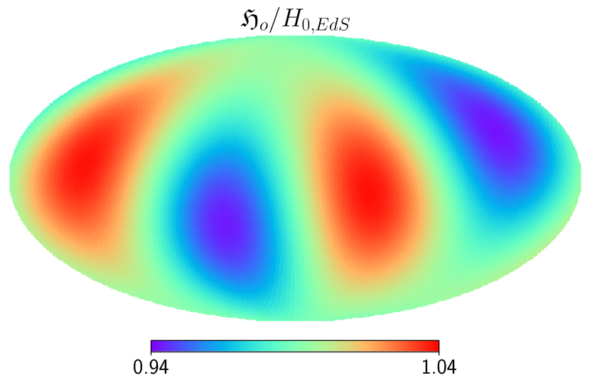
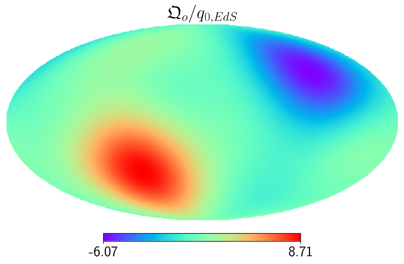
Figure 1: Sky maps for a single observer measured in directions of the $12\times N_{\rm side}^{2}$ HEALPix pixels with $N_{\rm side}=32$. The simulations have physical domain length of $L=12.8\,h^{-1}$ with a smoothing scale of $100\,h^{-1}$ Mpc. The left panel shows the effective Hubble parameter and the right panel shows the effective deceleration parameter. Both panels are normalised by their respective EdS values.

We use the data of 100 observers placed in random locations throughout two simulations from MH21. The two simulations both have numerical resolution $N=128$ (with the full cubic domain containing $N^{3}$ grid cells) but have different “smoothing scales”, such that individual grid cells have lengths $100\,h^{-1}$ Mpc and $200\,h^{-1}$ Mpc, giving domain lengths of $L=12.8\,h^{-1}$ Gpc and $L=25.6\,h^{-1}$ Gpc, respectively. These smoothing scales are chosen such that small-scale non-linearities have been explicitly excluded from the simulations. These chosen smoothing scales are motivated by observations which report a transition to statistical homogeneity at $\approx$ 100$h^{-1}$Mpc (Scrimgeour et al., 2012a). Incorporating such a smoothing scale in these kinds of calculations is necessary to ensure the regularity requirements of the general cosmography are satisfied in the calculations (see Heinesen, 2021, and also MH21).

For each observer, the effective cosmographic parameters have been calculated in the direction of $12\times N_{\rm side}^{2}$ HEALPix indices with with $N_{\rm side}=32$ — ensuring an

isotropic sky coverage for each observer (Górski et al., 2005).

In Figure 1 we show sky maps for the effective Hubble (left panel) and deceleration (right panel) parameters for a single observer in the NR simulation with smoothing scale $100h^{-1}$MPc (adapted from MH21). Both parameters are normalised by their respective EdS values, namely $H_{0,{\rm EdS}}=45$ km/s/Mpc and $q_{0,{\rm EdS}}=0.5$. For this observer, by eye we can see a quadrupolar anisotropy dominating the signal for the effective Hubble parameter — physically sourced from the shear tensor contribution in (7). This is to be expected for all observers in these simulations, since they are co-moving with a dust fluid and thus the acceleration $a_{\mu}$ term (contributing to the dipole) is subdominant.

For the effective deceleration parameter, the dipolar anisotropy appears to be dominant — physically sourced by gradients in the local expansion rate. While we might expect gradient terms to dominate in the coefficients (9), this is not obviously the case across all observers and will be dependent on their specific location. Thus, in the following section, we proceed to use this data for all observers to explicitly determine the dominant multipoles for each parameter.

3.2 Multipole Analysis

In this section, we work in Fourier space where the multipole components can be easily separated. First, we use the healpy package (Zonca et al., 2019; Górski et al., 2005) to calculate the angular power spectrum for multipole $\ell$ as

$${C_{\ell}}=\frac{1}{2\ell+1}\sum_{m}|{{a}_{\ell m}}|^{2},$$ (10)

using the healpy.anafast function. In the above, $a_{\ell m}$ are the spherical harmonic coefficients to the spherical harmonics $Y_{\ell m}$, which are defined from the expansion of a band-limited function $f$ on a sphere with angular coordinates $\theta,\phi$ as

$$f(\theta,\phi)=\sum^{\ell_{max}}_{\ell=0}\sum_{m}a_{\ell m}Y_{\ell m}(\theta,\phi).$$ (11)

We use $C_{\ell}$ to quantify the strength of each multipole component relative to the monopole. Specifically, for each observer, we calculate the ratio of the spherical harmonic coefficients, that is

$${\mathcal{R_{\ell}}=\sqrt{\frac{(2\ell+1)C_{\ell}}{C_{\ell=0}}}},$$ (12)

for $\ell>0$ in the numerator.

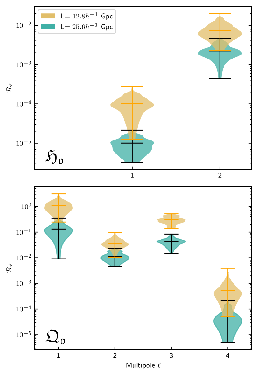
Figure 2: Relative ratios ($\mathcal{R}_{\ell}$) for each multipole relative to the monopole for the effective hubble ($\mathfrak{H_{o}}$) and deceleration ($\mathfrak{Q_{o}}$) parameters. The upper panel shows $\mathfrak{H_{o}}$, while $\mathfrak{Q_{o}}$ is shown below. Shaded regions represent an empirical distribution of the data, calculated using kernel density estimation (KDE). Results for two simulations of length $12.8h^{-}1$Gpc and $25.6h^{-}1$Gpc are shown in yellow and blue. The upper limits and medians are marked on the plots with horizontal lines. Note that $\mathfrak{H_{o}}$ only goes up to quadrupolar order, and $\mathfrak{Q_{o}}$ to a 16-pole due to the exact truncations in Eq. 7 and 8

This approach allows us to calculate the relative strength of each multipole with respect to the isotropic (monopole) component. Since $\mathfrak{R}$ and $\mathfrak{J}$ only enter the expansion (1) at third order in redshift, their contributions $d_{L}$ will be difficult to constrain with current data. Thus, in this work we focus on anisotropies in the effective Hubble and deceleration parameters. We present the corresponding analysis for the effective curvature and jerk parameters in Appendix A.

In Figure 2 we show this calculation for all 100 observers for both simulations for the effective Hubble and deceleration parameters. The shaded regions represent an empirical distribution of the data, calculated using kernel density estimation (KDE), with the median, upper, and lower limits displayed as horizontal bars.

We see the same qualitative trend for both simulations, however, for the simulation with $100\,h^{-1}$ Mpc smoothing scale we see generally larger amplitude anisotropic components. This is expected, as the smaller physical resolution allows for more small-scale structures to form, resulting in stronger local anisotropic effects. For the rest of this work, we consider this simulation as the fiducial case, since it contains the most realistic structure of the two.

For the effective Hubble parameter $\mathfrak{H}_{0}$, the dipole is on average four orders of magnitude smaller than the monopole term, with a median of $\mathcal{R}_{\ell=1}(\mathfrak{H})=1.029\times 10^{-4}$. However, the quadrupole has median value $\mathcal{R}_{\ell=2}(\mathfrak{H})=7.52\times 10^{-3}$. The effective deceleration parameter, $\mathfrak{Q}_{0}$, has a dipole with amplitude approximately $110\%$ that of the monopole, namely a median of $\mathcal{R}_{\ell=1}(\mathfrak{Q})=1.12$.The octopole of the effective deceleration parameter has amplitude of approximately $30\%$, or $\mathcal{R}_{\ell=3}(\mathfrak{Q})=0.314$.

From these results, we can reduce the degrees of freedom of the general cosmographic expansion by including only the dominant terms in each effective parameter.

The simplified version of Eq. (8) we use for the effective deceleration parameter which includes the monopole, dipole, and octopole contributions is

$$\mathfrak{Q}(e)\approx-1-\frac{1}{\mathfrak{H}^{2}(e)}\bigg{(}\overset{0}{\mathfrak{q}}+e^{\mu}\overset{1}{\mathfrak{q}}_{\mu}+e^{\mu}e^{\nu}e^{\rho}\overset{3}{\mathfrak{q}}_{\mu\nu\rho}\bigg{)}.$$ (13)

There are still many degrees of freedom even in this simplified expression. It will be difficult to constrain all three multipole components of $\mathfrak{Q}(e)$, and although the sky coverage of SNe has improved with Pantheon+, tightly constraining an octopole remains a challenge. For this reason, despite its potential significance, we neglect the octopole contribution and further simplify the expression to

$$\mathfrak{Q}(\boldsymbol{e})\approx-1-\frac{1}{\mathfrak{H}^{2}(\boldsymbol{e})}\bigg{(}\overset{0}{\mathfrak{q}}+e^{\mu}\overset{1}{\mathfrak{q}}_{\mu}\bigg{)}.$$ (14)

Similarly, for the effective Hubble parameter $\mathfrak{H}$, we use a simplified version of Eq. (7) in which we neglect the dipole term:

$$\mathfrak{H}(\boldsymbol{e})\approx\frac{1}{3}\theta-e^{\mu}e^{\nu}\sigma_{\mu\nu}.$$ (15)

Armed with a simplified version of the general cosmographic parametrisation of the luminosity distance, we now move toward constraining these anisotropies in observational data.

4 Observational data and methodology

Here we detail our methods for constraining the anisotropies discussed in the previous section using supernova data. We introduce the use of supernovae distances in constraining cosmology in Section 4.1, the statistical method we use in Section 4.2, the data sets we use in Section 4.3, the parametrisations we constrain in Section 4.5, and present our constraints themselves in Section 5.

4.1 Supernova distances

Type Ia supernovae (SNe) are a key part of the cosmic distance ladder (see, e.g. Goobar & Leibundgut, 2011, for a review). When calibrated, they act as standard candles for distance measurements via the relation

$$\mu\equiv m_{B}^{*}-M,$$ (16)

where $\mu$ is the distance modulus, $m_{B}^{*}$ is the corrected apparent magnitude of the SN and $M$ is its absolute magnitude. In this work, we will use $m_{B}^{*}$ from the Pantheon+ data set, which we introduce in Section 4.3 below. We refer the reader to Scolnic et al. (2021) for details of the corrections applied to $m_{B}$ in the public data set.

The luminosity distance, $d_{L}$ (in units of 10 parsec), is related to the distance modulus via

$$\mu=5\;\log\left(\frac{d_{L}}{10pc}\right),$$ (17)

which then allows us to constrain a chosen cosmological model via an analytic expression for the luminosity distance $d_{L}(z)$ using the observed redshift of the SNe. An option would be to use the $\Lambda\rm{CDM}$  distance-redshift relation, however, this would require input knowledge of the parameters for each component of the total energy-density of the Universe. Alternatively, at low redshift we can free ourselves from these constraints by using the cosmographic approach and thus adopting a general expansion history, as we outlined earlier in Section 2.2.

While the parameters describing the anisotropies in the luminosity distance are not degenerate with the SN Ia absolute $B$-band magnitude (see Section 4.5), the monopole of the Hubble expansion does suffer this degeneracy. This is well-known in SN Ia cosmology and is the reason that calibrators are required for local $H_{0}$ measurements (see, e.g. Riess et al., 2022; Freedman et al., 2019). In the fiducial analysis for constraining the anisotropies, we only use Hubble flow SNe Ia (i.e. with $z\geq 0.023$), hence, we cannot constrain the monopole, $H_{\rm mono}$. However, in attempt to assess the impact of anisotropies on the “Hubble tension”, in Section 5.3 we perform an analysis including the calibrator sample of SNe Ia in Pantheon+ and simultaneously constrain the monopole and quadrupole of the Hubble expansion.

4.2 Constrained $\chi^{2}$ method

In this work, we will place constraints on cosmological parameters (isotropic and anisotropic) by assuming a $\chi^{2}$ distribution;

$$\chi^{2}_{SN}=\Delta^{T}C_{SN}^{-1}\Delta$$ (18)

where the residual vector is $\Delta=m_{obs}-m_{th}$ (and $\Delta^{T}$ is its transpose vector), and $C_{SN}$ is the covariance matrix. We use pymultinest (Buchner et al., 2014), a python wrapper of Multinest (Feroz et al., 2009) to derive the posterior distribution of the parameters.

4.3 Pantheon+ Data

We use the new Pantheon+ (Scolnic et al., 2021) data set, a first analysis of which was presented in Brout et al. (2022) and Riess et al. (2022). This new Pantheon release has added six large SNe samples to the original data set (Scolnic et al., 2018), including 574 more light curves at $z<1$, as well as updated surveys due to a better understanding of the photometry. It contains 1701 light curves from 1550 SNe in the redshift range $0.001\leq z\leq 2.26$. In Figure 3 we show a skyplot of the directions of the Pantheon+ SNe in galactic coordinates, coloured according to their redshift in the heliocentric frame, $z_{\rm hel}$. The bottom panel shows a histogram of the number of SNe in the sample as a function of $z_{\rm hel}$. The sky-coverage is close to isotropic for the low-redshift SNe, however, the higher-redshift SNe are more strongly clustered on the sky. From the histogram, we can see that the data is dominated by the low redshift SNe.

As briefly mentioned in Section 2, the cosmographic expansion of luminosity distance with redshift as a parameter is strictly only convergent for $z<1$ (Cattoën & Visser, 2007). Since the Pantheon+ sample contains objects out to $z=2.26$, an upper-limit redshift cut might be necessary to ensure robust results. For our fiducial analysis, we use the same redshift cuts as was used for the cosmographic fits for $H_{0}$ and $q_{0}$ in Riess et al. (2022), namely, $0.023\leq z\leq 0.8$. This reduces our fiducial SNe sample to 1341 light curves.

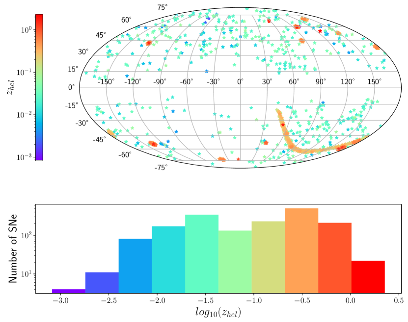
Figure 3: Skymap plot for the Pantheon+ dataset. Each star shows the location of a SNe on the sky, with colour showing heliocentric redshift. The lower panel shows the redshift distribution of the data.

4.4 Redshift Frames and Peculiar Velocity Effects

The choice of redshift frame has been shown to affect the strength of the constrained dipole in the deceleration parameter (e.g., D22,Rubin & Heitlauf (2020)). Different “redshift frames” are defined by applying some kind of peculiar velocity corrections to the raw redshifts that we observe, with the goal of transforming the observations into a different frame of reference. Most commonly, three redshift frames are used; the heliocentric frame (HEL), the CMB frame, and the Hubble diagram frame (HD). The heliocentric frame refers to redshift in the frame of the Sun, while the CMB frame redshifts have been corrected according to a single pointwise boost of our observations into the rest frame of the CMB. This boost is performed using our velocity inferred from the CMB dipole (assuming it is purely kinematic in nature). The HD frame redshifts are the CMB frame redshifts with peculiar velocity (PV) corrections applied to the SNeIa. These corrections are calculated based on density maps of the local Universe and linear perturbation theory, and estimate the PV of each SNe with respect to the CMB rest frame. For discussion on the effect of cosmological reference frames we refer the reader to Calcino & Davis (2017). In Section 5.1 and 5.2, we study the effect of varying the redshift frame on our resulting constraints.

4.5 Anisotropic distances for supernovae

Here we discuss our method to constrain the dominant multipoles we identified in Section 3.2 in the Pantheon+ data set.

For the effective deceleration parameter, as discussed in Section 3.2, we only constrain its dipole anisotropy. We re-parameterise Eq. (13) in a manner similar to D22;

$$\mathfrak{Q}(\boldsymbol{e})=q_{\rm mono}+q_{\rm dip}(\boldsymbol{e})\,\mathcal{F}(z,S_{\rm dip}),$$ (19)

where $\mathcal{F}(z,S_{\rm dip})$ is the scale dependence of the dipole and $q_{\rm dip}=\bf{q_{\rm dip}}\cdot\boldsymbol{e}$, where $\boldsymbol{e}$ is the direction of the supernova and ${\bf q_{\rm dip}}$ is the dipole vector. In order to quantify the strength of the dipole, we define the amplitude of the dipole at a given redshift as follows:

$$A_{d}=\Big{|}\Big{|}\frac{q_{\rm dip}({\bf e})}{q_{\rm mono}}\Big{|\Big{|}}\,\mathcal{F}_{(}z,S_{\rm dip}).\\$$ (20)

To further reduce the degrees of freedom and improve our fits, we also assume this dipole is aligned with the CMB dipole. Such an alignment might be expected based on the results of Heinesen & Macpherson (2021), where the authors found that the dipole in the effective deceleration parameter should be aligned with local density contrasts near the observer. Further, D22 and Colin et al. (2019) both tested the best-fit direction of this dipole and found it to coincide with the direction of the CMB dipole. Thus, we proceed by fixing the direction of ${\bf q}_{\rm dip}$ to be $(l,b)=(264.021,48.523)$° as found in Aghanim et al. (2020b).

The low-redshift anisotropic effects we are interested in are generated by the local clustering of matter, which leads to an anisotropic expansion of the local space-time. We expect such effects to decay as we move further away from the observer, i.e., to higher redshift. For these reasons, we choose to constrain an exponentially decaying anisotropy (see Colin et al., 2019, for fits using other forms of $\mathcal{F}$). The exponential decay function we use here is

$$\mathcal{F}(z,S)={\rm exp}\left(-\frac{z}{S}\right),$$ (21)

where we use a uniform prior for the decay scale, $S$, in line with Rahman et al. (2021) and D22.

Other works have similarly constrained a dipole in the deceleration parameter while assuming an isotropic $H_{0}$. However, as we see from Eq. (8), $\mathfrak{Q}_{0}$ is dependent on $\mathfrak{H}_{0}$. In this work, we incorporate the dominant quadrupole in the Hubble parameter. Specifically, we re-parameterise Eq. (15) as

$$\mathfrak{H}(\boldsymbol{e}) =H_{\rm mono}+H_{\rm quad}(\boldsymbol{e})\,\mathcal{F}(z,S_{q})$$ (22)

$$=H_{\rm mono}\bigg{\{}1+\bigg{[}\lambda_{1}\cdot{\rm cos}^{2}\theta_{1}+\lambda_{2}\cdot{\rm cos}^{2}\theta_{2}$$

$$\quad\quad-(\lambda_{1}+\lambda_{2})\cdot{\rm cos}^{2}\theta_{3}\bigg{]}\mathcal{F}(z,S_{q})\bigg{\}},$$

where $H_{\rm quad}(\boldsymbol{e})={\bf H_{\rm quad}}\cdot\boldsymbol{e}\,\boldsymbol{e}$ with ${\bf H_{\rm quad}}$ the quadrupole tensor, $\lambda_{1}$ and $\lambda_{2}$ (and $\lambda_{3}=\lambda_{1}+\lambda_{2}$) are the eigenvalues of the normalised quadrupole moment tensor ${\bf H_{\rm quad}}/H_{\rm mono}$, the $\theta_{i}$ (for $i=1,2,3$) are the angular separations between the location of the supernova and the quadrupole eigendirections, and $\mathcal{F}(z,S_{q})$ is the quadrupole decay function. We use the form of $\mathcal{F}$ given in Eq. (21) but we ensure the decay scale $S_{q}$ is distinct from that of the dipole in the deceleration parameter.

Due to the additional free parameters, it is difficult to constrain the direction of the quadrupole to any useful accuracy with current data sets. Thus, we assume the quadrupole in the Hubble parameter is aligned with that found in Parnovsky & Parnowski (2012) using the Revised Flat Galaxy Catalogue (RFGC) catalogue of 4236 galaxies. In this work, the authors studied the collective motion of local galaxies, fitting a dipole (bulk flow), a quadrupole (cosmic shear), and octupole component. They find eigenvectors of the quadrupole to have directions $(l,b)$ = (118, 85)°, (341, +4)° and (71, -4)°. This eigendirection was also used in the constraints on the quadrupole in the Hubble parameter in D22, where the authors found the constraints to be insensitive to the chosen direction.

To assess the overall amplitude of the quadrupole in the Hubble parameter, we calculate the amplitude of the quadrupole component of $\mathfrak{H}(\boldsymbol{e})$ in the same way as D22, and similar to the dipole amplotide defined in Eq. 20, namely, as the norm of the tensor ${\bf H_{\rm quad}}$ multiplied by the decay function $\mathcal{F}$,

$$A_{q} =||{\bf H_{\rm quad}}||\,\mathcal{F}_{\rm quad}(z,S)$$ (23)

$$=\sqrt{\lambda_{1}^{2}+\lambda_{2}^{2}+\left(\lambda_{1}+\lambda_{2}\right)^{2}}\,\mathcal{F}_{\rm quad}(z,S_{q}),$$ (24)

for some redshift scale $z$.

5 Anisotropy in supernova data

In this section we present our constraints on local anisotropies in the Pantheon+ data set, motivated by those we identified in the numerical relativity simulations. In Section 4.4 we discuss the redshift frames of the data we use, in Section 5.1 we present our constraints on the dipole in the deceleration parameter, and in Section 5.2 we present constraints on the quadrupole in the Hubble parameter. We also present constraints on the isotropic Hubble parameter, $H_{0}$, in Section 5.3 and the resulting implications for the “Hubble tension”.

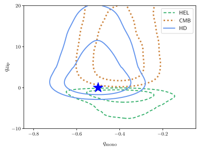
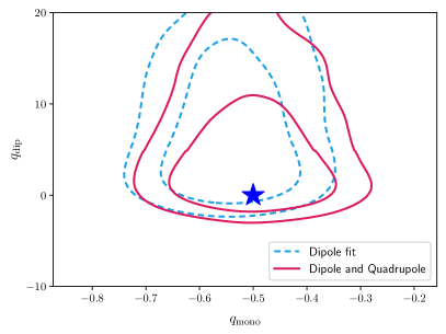
Figure 4: Left panel: Results for the dipole in various redshift frames. The blue solid line shows our fiducial analysis, the Hubble diagram frame, the green dashed line shows the CMB frame and the yellow dotted line shows the heliocentric frame. Right panel: Constraints on the dipole in the effective deceleration parameter when fitting only for a dipole (blue dashed) vs. also fitting for a quadrupole in the Hubble parameter with decay factor $S_{q}=0.06/\ln(2)$(pink solid). The blue star marks isotropy. Contours represent the $1\sigma$ and $2\sigma$ –-constraints.

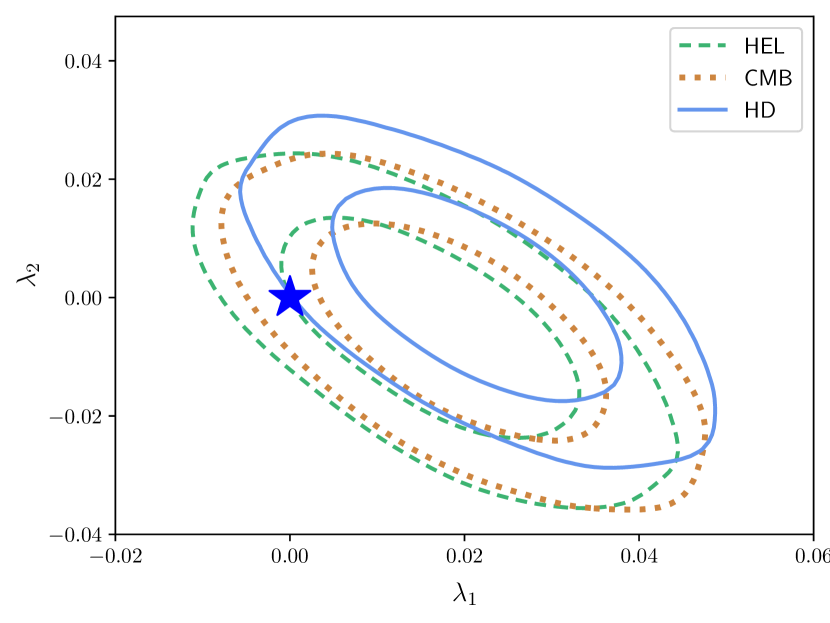
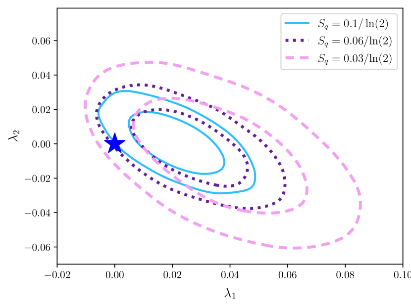
Figure 5: Left panel: Constraints on the quadrupole eigenvalues in various redshift frames. The blue solid line shows our fiducial analysis, the Hubble diagram frame, the green dashed line shows the CMB frame and the yellow dotted line shows the heliocentric frame. The decay scale is set to $S_{q}=0.1/\ln(2)$. The blue star marks isotropy. Contours represent the $1\sigma$ and $2\sigma$ –-constraints. Right panel:Constrains on the eigenvalues of the quadrupole of the effective Hubble parameter when parameterised at fixed decay scales, $S_{q}$. The blue star marks isotropy. Contours represent the $1\sigma$ and $2\sigma$ constraints. All cases are inconsistent with isotropy.

5.1 Dipole of the deceleration parameter

We begin our analysis by fitting the dipole in the deceleration parameter of the form given in Eq. (19). In this section, we will consider cases both with and without an additional contribution from a quadrupole in the Hubble parameter. As discussed in Section 4.5, we fix the direction of the dipole to coincide with the CMB dipole, as constrained by Planck Collaboration et al. (2020a). The dependence of the resulting dipole amplitude on this fixed direction has been explored in D22 and Colin et al. (2019) and in both cases the CMB dipole direction was the best fit for the data sets. We do not anticipate this dependence to differ in the case of the Pantheon+ data set.

First, we will constrain the dipole in the deceleration parameter in all three redshift frames introduced in Section 4.4, while simultaneously constraining a quadrupole in the Hubble parameter. In this section we present the constraints on $\mathfrak{Q}(e)$ only, and present the constraints on quadrupole parameters in the section 5.2. In the left panel of Figure 4 we show constraints in the $q_{\rm dip}$-$q_{\rm mono}$ plane for heliocentric frame (dotted brown contours), CMB frame (dashed green contours), and HD frame (solid blue contours) redshifts. Contours represent the 1- and $2\sigma$ constraints for all fits. The blue star marks isotropy within $\Lambda$CDM, namely $q_{\rm mono}=-0.55$ and $q_{\rm dip}=0$. We summarise the central values and 1$\sigma$ uncertainties of these constraints for all three frames in Table 1. When quoting $\sigma$ deviations from isotropy throughout this work, we do not assume a Gaussian distribution of our parameter constraints. Instead, we use the inverse error function to convert a given percentile to a significance in multiples of $\sigma$ (in a similar manner to D22).

In the HD redshift frame, we find consistency with isotropy at $<1\sigma$. However, in the CMB frame we find inconsistency with isotropy at $3.17\sigma$. Our constraints for the CMB and HD frame redshifts are roughly consistent with D22, however, our heliocentric frame constraints are consistent with isotropy at $\lesssim 2\sigma$ while both D22 and Colin et al. (2019) detect a dipole at $>2\sigma$. This difference can most likely be attributed to the addition of a quadrupole in the Hubble parameter in our analysis, since in both D22 and Colin et al. (2019) the authors considered a dipole-only fit. It is perhaps the case that some of the anisotropy present in distances in the heliocentric frame is being absorbed into the quadrupolar anisotropy in $\mathfrak{H}(e)$ in our analysis.

Frame	$q_{\rm mono}$	$q_{\rm dip}$	Dipole significance
CMB	$-0.405\pm 0.089$	$9.6^{+4.0}_{-6.9}$	3.17 $\sigma$
HD	$-0.503\pm 0.088$	$4.5^{+1.9}_{-5.4}$	-
HEL	$-0.391\pm 0.091$	$-2.36^{+1.6}_{-0.43}$	$>2\sigma$

Table 1: Summary of constraints on the dipole in the deceleration parameter for the three redshift frames used in the Pantheon+ data set. All results were obtained using the $\chi^{2}$ method and significances were found using the highest posterior density interval and the error function, as in D22

Next, we will compare our constraints on the dipole in the HD frame both with and without a quadrupole contribution in the Hubble parameter. The right panel of Figure 4 shows our constraints assuming only a dipole in the deceleration parameter (dashed blue contours) and when also allowing for a quadrupole in $\mathfrak{H}$ with decay scale $S_{q}=0.06/{\rm ln}(2)$ (pink solid contours; see Section 5.2 below for constraints on the quadrupole and a discussion of decay scales). Our constraints for the dipole only fit are are $q_{\rm mono}=-0.541\pm 0.085$, $q_{\rm dip}=7.0^{+3.8}_{-7.2}$ , to be compared with the HD case in Table 1, namely, we find a small shift to larger values of both $|q_{\rm mono}|$ and dipole magnitude for the dipole-only case. Although, this shift is $<1\sigma$ and so we conclude that the two cases are consistent with one another. We also note that our results, for a similar selection of the redshift range, are consistent with a recent study by Sorrenti et al. (2022). From Eq. 20, using 1$\sigma$ constraints and a redshift of 0.035 and decay scale $S_{\rm dip}=0.0367$, we find a maximum amplitude of $417\%$, and an amplitude of $345\%$ when using the median values. While not directly comparable due to having to select a redshift, this is in agreement with our simulation value of $110\%$ For both cases, our constraints on the deceleration parameter are also consistent with $\Lambda$CDM to within $1\sigma$.

5.2 Quadrupole in the Hubble parameter

$S_{q}$	$\lambda_{1}$	$\lambda_{2}$	$A_{q}$
$0.1/{\rm ln}(2)$	$0.021\pm{0.011}$	${3.15\times 10^{-5}}\pm 0.012$	$2.68\%$
$0.06/{\rm ln}(2)$	$0.026\pm{0.014}$	$-0.0021\pm{0.014}$	$2.88\%$
$0.03/{\rm ln}(2)$	$0.037\pm 0.02$	$-0.0072\pm{0.022}$	$2.85\%$

Table 2: Constraints on the quadrupole in $H_{0}$ for the fiducial case in the HD frame (while also fitting for a dipole in $\mathfrak{Q}(\boldsymbol{e})$). The maximum allowed amplitude at $1\sigma$, $A_{q}$, is calculated according to Eq. (24) at a redshift of $z=0.035$, corresponding to scales of $\approx 100\,h^{-1}$ Mpc.

We constrain the effective Hubble parameter using the form given in Eq. (22). Here, we will only quote results from the joint fit of a dipole in the deceleration parameter and a quadrupole in the Hubble parameter. We constrain the quadrupole eigenvalues $\lambda_{1}$ and $\lambda_{2}$ and initially fit with the decay scale $S_{q}$ as a free parameter in the analysis. However, we find $S_{q}$ to be largely unconstrained. Thus, we proceed to constrain the quadrupole eigenvalues for three values of the decay scale as used in D22. Namely, we choose $S_{q}=0.1/$ln(2), $S_{q}=0.06/$ln(2), and $S_{q}=0.03/$ln(2). This corresponds to a halving of the quadrupole amplitude at redshifts of $z=0.1,0.06,$ and $0.03$, respectively. As mentioned in Section 4.5, to further reduce the degrees of freedom we fix the quadrupole direction to that found by Parnovsky & Parnowski (2012) in the RFGC catalogue. Specifically, we fix the eigenvectors of the quadrupole to directions $(l,b)$ = (118, 85)°, (341, +4)° and (71, -4)°. The effect of varying the quadrupole direction was explored in D22, where the authors found no significant improvement for different choices of eigenvectors.

As in D22, we also test the impact of redshift frame on the quadrupole constraints. In the left panel of Figure 5, we show constraints on $\lambda_{1}$ and $\lambda_{2}$ for the heliocentric (HEL) frame (dotted brown contours), CMB frame (dashed green contours), and HD frame (solid blue contours) redshifts, where the blue star marks isotropy ($\lambda_{1}=\lambda_{2}=0$). These three constraints use a fixed decay scale of $S_{q}=0.1/{\rm ln}(2)$. As in D22, we see very little shifting of the quadrupole posterior with redshift frame. We note however that in the case of the HD frame redshifts, our constraints are inconsistent with isotropy at $\sim 2\sigma$, while the heliocentric and CMB frame redshifts yield results consistent with isotropy at < 2$\sigma$. The CMB redshifts are calculated from the heliocentric redshifts using a single pointwise boost towards the CMB — which is predominantly a dipolar correction. Thus,we might expect some shift in the detected dipole in the deceleration parameter in the left panel of Figure 4 (when moving from HEL to CMB redshifts). Although, we might not necessarily expect the CMB frame redshifts to still contain a dipole signal at $\sim 2\sigma$.

We would not expect this single boost to impact a quadrupole in the field of local SNe, which is what we find in the left panel of Figure 5 (i.e., little to no shift moving from HEL to CMB redshifts). However, the next step to get from CMB to HD redshifts is to apply individual corrections to each SNe according to estimates of the local PV field. Such a correction is more extensive than a single boost, and thus in general should contain both dipole and quadrupole components (as well as higher-order multipoles). This is what we find, namely, we see both a change in the dipole we detect (moving from CMB to HD redshifts in the left panel of Figure 4) and a small, but noticeable, shift in the quadrupole (moving from CMB to HD redshifts in the left panel of Figure 5). This is perhaps surprising, as it implies including PV corrections, that is corrections of bulk flows, brings us further from the isotropic model by slightly pushing the quadrupole to higher values. However, we would expect the source anisotropies to be due to bulk flows around an FLRW background, and so the corrections to have the opposite effect. For the rest of this section, we take the fiducial case to be the HD frame redshifts, since these are most commonly used in SNe analyses.

Next, we will assess the quadrupole eigenvalues when varying the fixed decay scale $S_{q}$. In the right panel of Figure 5, we show constraints on the two independent eigenvalues $\lambda_{1}$ and $\lambda_{2}$ for a decay scale of $S_{q}=0.1/$ln(2) with solid blue contours, a scale of $S_{q}=0.06/$ln(2) with dotted purple contours, and $S_{q}=0.03/$ln(2) with pink dashed contours. The blue star again marks isotropy, i.e., $\lambda_{1},\lambda_{2}$ = 0. For all cases we consider, we find a quadrupole signal which is inconsistent with isotropy at the $\sim 2\sigma$ level. We calculate upper ($1\sigma$) limits on the amplitude of the quadrupole using Eq 24 for all three cases, and find the largest amplitude in the case of a decay scale of $S_{q}=0.06/$ln(2), namely, we place a limit of a $\lesssim$ $2.88\%$ quadrupole strength at $z=0.035$. In Table 2 we present our exact constraints together with $1\sigma$ uncertainties. This is in agreement this with the strength we predicted from simulations in Section 3.2, $\mathcal{R}_{\ell=2}(\mathfrak{H})=7.52\times 10^{-3}=0.752\%$.

While all contours are inconsistent with isotropy at $\sim 2\sigma$, this deviation is only due to a non-zero $\lambda_{1}$ at 2$\sigma$, while $\lambda_{2}$ remains consistent with zero at 1$\sigma$ for all three cases of fixed decay scale (and also for all three redshift frames in the left panel of Figure 5). Smaller values of $S_{q}$ imply a faster decay of $\mathcal{F}(z,S_{q})$, and thus the quadrupole anisotropy being constrained is present at lower redshifts. We find that reducing the decay scale shifts the distribution of $\lambda_{1}$ slightly towards larger values (though all distributions are consistent within 1$\sigma$). This is somewhat intuitive, as we expect these local anisotropic effects to be larger closer to the observer, i.e., at lower redshifts. We also see a widening of the constraints for progressively smaller decay scales, which again might be expected because as we sharpen the decline of $\mathcal{F}(z,S_{q})$, we are also effectively constraining the anisotropy using less SNe. Ideally, we would require a data set with more low-redshift objects to more tightly constrain these models with small decay scales.

D22 found the quadrupole in the Hubble parameter — constrained using an identical method to that which we use here, though with the original Pantheon data set — to be consistent with isotropy for all cases at $\sim 1\sigma$ using the same set of fixed decay scales as we show in the right panel of Figure 5. While our constraints are roughly consistent with those of D22 to within $\sim 1\sigma$ for all three decay scales, we do see a shift to larger $\lambda_{1}$ values with the updated Pantheon+ data set, as well as a tightening of the contours.

Recently, Kalbouneh et al. (2022) defined a new observable based on a spherical harmonic decomposition of the observed Hubble expansion, correct to linear order in redshift. While the authors claim detection of a significant quadrupole in the Cosmicflows-3 all-sky galaxy catalogue (Tully et al., 2016), they report a null detection in the Pantheon sample (Scolnic et al., 2018) as was found in D22. Such an analysis using updated data sets, such as Cosmicflows-4 (Tully et al., 2022) and Pantheon+, would provide a valuable comparison and potential validation of the significant quadrupole we find in this work. The methods and data sets used in Kalbouneh et al. (2022) differ from our work such that a direct comparison of the quadrupoles we find is not straightforward. However, in the next section we will naively compare to their quoted maximal variance of $H_{0}$ across the sky and its relevance to the “Hubble tension”.

5.3 Implications for the Hubble tension

Current measurements of the local Hubble expansion within the FLRW model, $H_{0}$, using the Pantheon+ data set now lie in 5$\sigma$ tension with $\Lambda\rm{CDM}$ predictions based on measurements of CMB anisotropies (Riess et al., 2022; Aghanim et al., 2020b). This is commonly referred to as the “Hubble tension” and no one resolution is widely accepted. In this section, we explore the significance of our results with respect to measurements of the Hubble parameter.

5.3.1 Impact on the monopole

First, we assess the impact of accounting for a quadrupole on the inferred value of the monopole of the Hubble parameter, i.e., for a measurement of the local Hubble constant $H_{0}$. We found a quadrupolar variance of the Hubble parameter across the sky at 2$\sigma$ significance. For a catalogue of SNe with incomplete sky coverage, an inference of the isotropic Hubble parameter $H_{0}$ might be expected to be impacted by this anisotropy. Such an effect could result in a locally higher value of $H_{0}$ if the catalogue preferentially samples directions of maximal quadrupole amplitude (see also Macpherson & Heinesen, 2021, for a discussion on this).

As briefly mentioned in Section 4.1, SNe Ia alone cannot constrain the monopole in the Hubble parameter due to the degeneracy between $H_{\rm mono}$ and the absolute luminosity of the SN Ia, $M$. Including the calibrator SNe Ia — which are also distributed as part of the SH0ES and Pantheon+ data release — allows us to break this degeneracy and thus constrain $H_{\rm mono}$. This calibrator sample includes a total of 37 galaxies with distances measured using Cepheid variables, hosting a total of 42 SNe Ia. We will first simultaneously constrain $H_{\rm mono}$, $M$, and the parameters for the quadrupole in the Hubble parameter, i.e. $\lambda_{1}$ and $\lambda_{2}$. We show our resulting constraints on the monopoles of the deceleration and Hubble parameters in Figure 6. We use the same three fixed decay scales as in Section 5.2, and for comparison, we show a purely isotropic constraint on $H_{\rm mono}$ with black dashed contours (i.e., a fit with fixed $\lambda_{1}=\lambda_{2}=0$). The central value of $H_{\rm mono}$ is consistent across all anisotropic fits, and does not differ significantly from the isotropic case. We find the largest difference between the central values of the anisotropic fits and the isotropic $H_{\rm mono}$ to be 0.30 km s^-1 Mpc^-1 in the case of $S_{q}=0.1/\ln(2)$, where $H_{0}=73.40\pm 1.02$. Thus, we conclude that despite finding a 2$\sigma$ significant quadrupole, accounting for this anisotropy in an inference of $H_{\rm mono}$ does not shift the central value enough to account for the $\sim 5$ km s^-1 Mpc^-1 Hubble tension discrepancy.

5.3.2 Maximal sky variance of the Hubble parameter

Kalbouneh et al. (2022) studied the maximal deviation in $H_{0}$ as measured using two populations of Pantheon SNe in antipodal directions on the sky. While the authors did not find a significant quadrupole feature in the Pantheon sample, they did find a dipolar feature in the distance modulus of these SNe (which can most likely be attributed to anisotropy in the effective deceleration parameter, see Heinesen, 2021; Heinesen & Macpherson, 2021). For this sample, they find the maximal variance to be $\Delta H_{0}=2.4\pm 1.1$ km s^-1 Mpc^-1 after applying PV corrections (i.e. using HD frame redshifts). While here we constrained only a quadrupole anisotropy in the Hubble parameter, as is expected, we might still compare the maximal variance across the sky found by Kalbouneh et al. (2022) to our own given the constraints presented in Section 5.2. To do this we use the constraints on $\lambda_{1}$ and $\lambda_{2}$ given in Table 2 for the three decay scales studied, and calculate $\mathfrak{H}(\boldsymbol{e})$ using Eq. 22. We study two different cases of directions ($\boldsymbol{e}$) and redshifts ($z$ in the decay scale $\mathcal{F}(z,S_{q})$) in calculating $\mathfrak{H}(\boldsymbol{e})$. First, we consider $\boldsymbol{e}$ given by the directions of HEALPix indices (with $N_{\rm side}=4$) and the separations $\theta_{i}$ are thus the sky separation between each HEALPix index and our fixed quadrupole direction. In this first case, we consider a single redshift value of $z=0.035$ to quantify the variance in $\mathfrak{H}$ at $\sim 100\,h^{-1}$ Mpc scales. Second, we consider $\boldsymbol{e}$ given by the directions of the Pantheon+ SNe and $\mathcal{F}(z,S_{q})$ calculated using each SNe redshift, which lies in the range 0.023<$z$<0.8. This second case gives us a quantification of the variance in $\mathfrak{H}$ across the sky for the Pantheon+ SNe sample. In both cases, we then calculate $\Delta\mathfrak{H}(\boldsymbol{e})\equiv\mathfrak{H}(\boldsymbol{e})_{\rm max}-\mathfrak{H}(\boldsymbol{e})_{\rm min}$ for an assumed $H_{\rm mono}=73.5$ km s^-1 Mpc^-1 (consistent with our fits in Figure 6).

We show the variances we find in Table 3 for both sample cases (single redshift or Pantheon+ redshift range) for all decay scale models we have constrained. All show a $\sim 2--2.5$ km s^-1 Mpc^-1 sky-variance of the Hubble parameter, with upper limits closer to $\sim 4$ km s^-1 Mpc^-1. All of our results are consistent with the variance found in Kalbouneh et al. (2022) using the Pantheon sample, although the authors here used a more restricted, low-$z$ sample of $0.01<z<0.05$ due to their first-order expression.

$S_{q}$	$z$	$\Delta\mathfrak{H}(\boldsymbol{e})$ (km/s/Mpc)
$0.1/{\rm ln}(2)$	0.035	$2.356^{+1.802}_{-1.185}$
	0.023 < z < 0.8	$2.329^{+1.693}_{-1.152}$
$0.06/{\rm ln}(2)$	0.035	$2.377^{+2.010}_{-1.040}$
	0.023 < z < 0.8	$2.406^{+1.999}_{-1.002}$
$0.03/{\rm ln}(2)$	0.035	$2.122^{+1.853}_{-0.679}$
	0.023 < z < 0.8	$2.471^{+1.948}_{-0.785}$

Table 3: Maximal sky variance of the anisotropic Hubble parameter, $\Delta\mathfrak{H}(\boldsymbol{e})$, for our best-fit quadrupole constraints given in Table 2. All variances are calculated at a scale of $z=0.035$, corresponding approximately to $100\,h^{-1}$ Mpc.

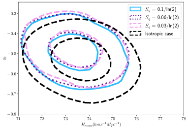
Figure 6: The constraints on the monopole of the Hubble parameter and the deceleration parameter with and without including anisotropy. Black dashed contours show an isotropic fit to the monopoles, and the coloured contours show constraints on the monopoles when accounting for anisotropy (for three models for the decay scale, as indicated in the legend).

6 Conclusions

The local Universe is highly inhomogeneous and anisotropic due to the presence of late-time nonlinear structures. This naturally leads to an anisotropic local expansion of space-time, which could impact cosmological inferences which assume isotropy. In this work, our goal was to constrain theoretically-motivated anisotropies in low-redshift supernova data.

We used the generalised cosmographic expansion of the luminosity distance from Heinesen (2021) and the simulation data from Macpherson & Heinesen (2021) to predict the dominant anisotropic signatures in nearby luminosity distances. To do this, we considered a set of two simulations, with different “smoothing scales”, each containing 100 randomly-placed synthetic observers. Each observer has a full-sky distribution of the effective cosmological parameters defined in Heinesen (2021), on which we performed a multipole expansion to determine the dominant contributions. We found the dipole and octopole to be the dominant multipoles in the effective deceleration parameter and found the quadrupole to dominate the effective Hubble parameter for all cases we studied. Within the simulation with smoothing scale of $100\,h^{-1}$ Mpc, we found the quadrupolar signal in the Hubble parameter has a strength of $5.65\times 10^{-3}\%$ with respect to the monopole on average over all observers, while the dipole in the deceleration parameter has strength $\sim 53\%$ on average.

Next, we constrained these dominant anisotropies using the new Pantheon+ SNe data set (Scolnic et al., 2021). In the rest frame of the CMB, we found an $3.17\sigma$ significant dipole with magnitude $q_{\rm dip}=9.6^{+4.0}_{-6.9}$. When correcting SNe redshifts for their peculiar velocities (i.e. using HD frame redshifts), the significance is removed and we find consistency with $\Lambda\rm{CDM}$. (see also, Sorrenti et al., 2022) Interestingly, we found a $1.96\sigma$ significant quadrupole in the Hubble parameter even after applying all peculiar velocity corrections. We place a new $1\sigma$ upper limit on the maximum amplitude of a quadrupole in the Hubble expansion of $2.88\%$.

Anisotropies in the Hubble expansion are of particular interest for the Hubble tension (Macpherson & Heinesen, 2021). If the Hubble parameter varies depending on which direction we observe, studies assuming an isotropic Hubble expansion could be biased in their results. We performed an analysis in which we constrained the monopole of the Hubble parameter — by also including calibrator SNe — along with the anisotropic components, as shown in Fig. 6. Allowing for such an anisotropic variance results in a monopole of the Hubble parameter of $73.40\pm 1.02$ km s^-1 Mpc^-1. This corresponds to a maximum shift of $\sim 0.30$ km s^-1 Mpc^-1 (for the cases considered here) with respect to the isotropic fit, and thus it is unlikely that such an anisotropic variance can account for the observed difference in local inferences of the Hubble parameter.

Finally, we note that our findings are specific to models within the cosmographic framework, and the effects we discuss arising in the simulation source purely from clustering effects. Therefore this work is not a general constraint on any potential anisotropy, especially e.g. anisotropic cosmological models such as e.g. Lavinto et al. (2013); Constantin et al. (2022).

Data Availability

All Python packages and the Pantheon+ data used in this work are publicly available. Specific code used in our analysis can be made available upon reasonable request to the corresponding author.

Appendix A The Curvature and Jerk Parameters

Here we present our results on the level of anisotropy measured in the effective curvature, $\mathfrak{R}$, and jerk, $\mathfrak{J}$, parameters in the NR simulations presented in Section 3.1. The parameters $\mathfrak{R}$ and $\mathfrak{J}$ are defined in Eq. (6c) and 6b respectively. Their full multipole expansions are given in Heinesen (2021). Here we perform the same multipole analysis on these parameters as we performed in Section 3.2 for the Hubble and deceleration parameters.

Figure 7 shows violin plots representing the strength of a multipole relative to the monopole, namely $\mathcal{R}_{\ell}$, as a function of the multipole number $\ell$. Yellow regions represent the distribution over 100 observers placed in the simulation with box length $L=12.8\,h^{-1}$Gpc, and green regions represent the same number of observers in the simulation with box length $L=25.6\,h^{-1}$Gpc. The top panel shows results for the effective jerk parameter and the bottom panel shows results for the effective curvature parameter. Horizontal bars in each distribution represent the maximum, mean, and minimum (top to bottom, respectively) value across the distribution of observers, and the width of each distribution represents the number of observers with that value of $\mathcal{R}_{\ell}$.

As we also saw in Section  3.2, in general, the $L=12.8h^{-1}$ Gpc simulation shows a trend of larger amplitude anisotropic effects. This is to be expected since this simulation has a smaller smoothing scale and thus higher density contrasts in general. We can also see that in both the effective jerk and curvature parameters, some higher-order multipole terms dominate over the isotropic terms (i.e. they have $\mathcal{R}_{\ell}>1$). Specifically, the median ${\mathcal{R}_{\ell=1}(\mathfrak{R})=5.01}$ and ${\mathcal{R}_{\ell=3}(\mathfrak{R})=1.30}$ . Similarly for $\mathfrak{J}_{o}$, we see the median value of the ratio for the quadrupole is $\mathcal{R}_{\ell=1}(\mathfrak{J})=1.12$, .

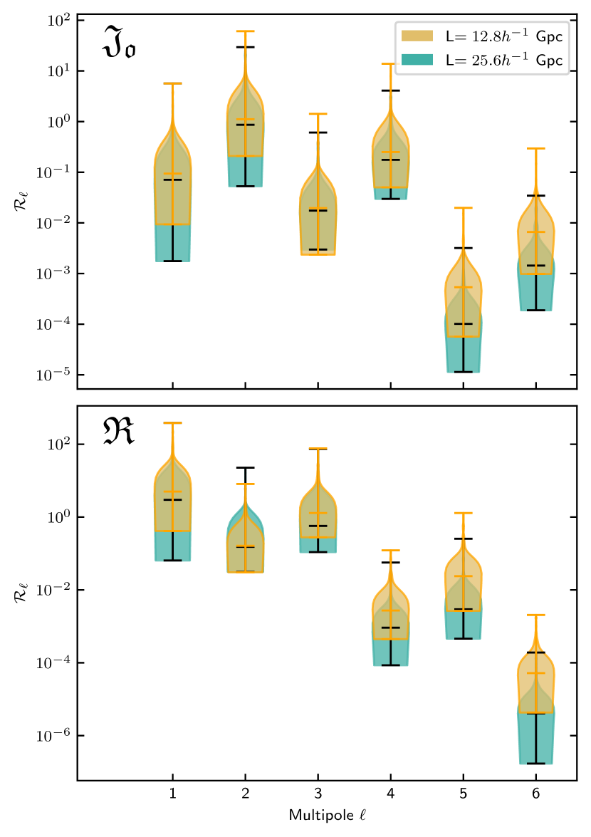
Figure 7: Relative ratios $\mathcal{R}_{\ell}$ for each multipole relative to the monopole for the effective jerk ($\mathfrak{J}_{o}$) and curvature ($\mathfrak{R}$) parameters. We show $\mathfrak{J}_{o}$ in the upper panel and in the bottom panel we show $\mathfrak{R}$. Shaded regions represent an empirical distribution of the data, calculated using kernel density estimation (KDE). Results for two simulations of length $12.8\,h^{-}1$ Gpc and $25.6\,h^{-}1$ Gpc are shown in yellow and blue, respectively. The upper limits, medians, and minimum values are marked on the plots with horizontal lines.

References

- Abbott et al. (2022) Abbott T. M. C., et al., 2022, Phys. Rev. D, 105, 023520
- Abdalla et al. (2022) Abdalla E., et al., 2022, Journal of High Energy Astrophysics
- Ade et al. (2019) Ade P., et al., 2019, Journal of Cosmology and Astroparticle Physics, 2019, 056–056
- Aghanim et al. (2020a) Aghanim N., et al., 2020a, Astronomy & Astrophysics, 641, A1
- Aghanim et al. (2020b) Aghanim N., et al., 2020b, Astronomy & Astrophysics, 641, A6
- Alonso et al. (2015) Alonso D., Salvador A. I., Sánchez F. J., Bilicki M., García-Bellido J., Sánchez E., 2015, Monthly Notices of the Royal Astronomical Society, 449, 670
- Aluri et al. (2022) Aluri P. K., et al., 2022, arXiv e-prints, p. arXiv:2207.05765
- Andrade et al. (2018) Andrade U., Bengaly C. A. P., Santos B., Alcaniz J. S., 2018, ApJ, 865, 119
- Appleby et al. (2015) Appleby S., Shafieloo A., Johnson A., 2015, The Astrophysical Journal, 801, 76
- Bengaly (2016) Bengaly C. A. P. J., 2016, J. Cosmology Astropart. Phys., 2016, 036
- Bennett et al. (2003) Bennett C. L., et al., 2003, ApJS, 148, 1
- Bolejko et al. (2016) Bolejko K., Nazer M. A., Wiltshire D. L., 2016, Journal of Cosmology and Astroparticle Physics, 2016, 035–035
- Brout et al. (2022) Brout D., et al., 2022, The Pantheon+ Analysis: Cosmological Constraints, doi:10.48550/ARXIV.2202.04077, https://arxiv.org/abs/2202.04077
- Buchner et al. (2014) Buchner J., et al., 2014, A&A, 564, A125
- Cai & Tuo (2012) Cai R.-G., Tuo Z.-L., 2012, Journal of Cosmology and Astroparticle Physics, 2012, 004
- Calcino & Davis (2017) Calcino J., Davis T., 2017, JCAP, 01, 038
- Cattoën & Visser (2007) Cattoën C., Visser M., 2007, Classical and Quantum Gravity, 24, 5985
- Chang et al. (2018) Chang Z., Lin H.-N., Sang Y., Wang S., 2018, Monthly Notices of the Royal Astronomical Society, 478, 3633
- Clarkson & Umeh (2011) Clarkson C., Umeh O., 2011, Classical and Quantum Gravity, 28, 164010
- Colin et al. (2011) Colin J., Mohayaee R., Sarkar S., Shafieloo A., 2011, Monthly Notices of the Royal Astronomical Society, 414, 264–271
- Colin et al. (2019) Colin J., Mohayaee R., Rameez M., Sarkar S., 2019, A&A, 631, L13
- Constantin et al. (2022) Constantin A., Harvey T. R., von Hausegger S., Lukas A., 2022, Spatially Homogeneous Universes with Late-Time Anisotropy, http://arxiv.org/abs/2212.03234
- Dhawan et al. (2022) Dhawan S., Borderies A., Macpherson H. J., Heinesen A., 2022, arXiv preprint arXiv:2205.12692
- Efstathiou (2021) Efstathiou G., 2021, Monthly Notices of the Royal Astronomical Society, 505, 3866–3872
- Ellis et al. (1985) Ellis G. F. R., Nel S. D., Maartens R., Stoeger W. R., Whitman A. P., 1985, Physics Reports, 124, 315–417
- Feindt (2013) Feindt U. e. a., 2013, A&A, 560, A90
- Feroz et al. (2009) Feroz F., Hobson M. P., Bridges M., 2009, Monthly Notices of the Royal Astronomical Society, 398, 1601–1614
- Freedman et al. (2019) Freedman W. L., et al., 2019, ApJ, 882, 34
- Gibelyou & Huterer (2012) Gibelyou C., Huterer D., 2012, Monthly Notices of the Royal Astronomical Society, 427, 1994
- Goobar & Leibundgut (2011) Goobar A., Leibundgut B., 2011, Annual Review of Nuclear and Particle Science, 61, 251
- Górski et al. (2005) Górski K. M., Hivon E., Banday A. J., Wandelt B. D., Hansen F. K., Reinecke M., Bartelmann M., 2005, ApJ, 622, 759
- Heinesen (2021) Heinesen A., 2021, Journal of Cosmology and Astroparticle Physics, 2021, 008
- Heinesen & Macpherson (2021) Heinesen A., Macpherson H. J., 2021, arXiv:2111.14423 [astro-ph, physics:gr-qc]
- Heinesen & Macpherson (2022) Heinesen A., Macpherson H. J., 2022, J. Cosmology Astropart. Phys., 2022, 057
- Hogg et al. (2005) Hogg D. W., Eisenstein D. J., Blanton M. R., Bahcall N. A., Brinkmann J., Gunn J. E., Schneider D. P., 2005, ApJ, 624, 54
- Hounsell et al. (2018) Hounsell R., et al., 2018, ApJ, 867, 23
- Huterer et al. (2015) Huterer D., Shafer D. L., Schmidt F., 2015, Journal of Cosmology and Astroparticle Physics, 2015, 033
- Javanmardi & Kroupa (2017) Javanmardi B., Kroupa P., 2017, A&A, 597, A120
- Kalbouneh et al. (2022) Kalbouneh B., Marinoni C., Bel J., 2022, The multipole expansion of the local expansion rate, doi:10.48550/ARXIV.2210.11333, https://arxiv.org/abs/2210.11333
- Kalus, B. et al. (2013) Kalus, B. Schwarz, D. J. Seikel, M. Wiegand, A. 2013, A&A, 553, A56
- Kristian & Sachs (1966) Kristian J., Sachs R. K., 1966, ApJ, 143, 379
- Lavinto et al. (2013) Lavinto M., Räsänen S., Szybka S. J., 2013, JCAP, 12, 051
- Macpherson & Heinesen (2021) Macpherson H. J., Heinesen A., 2021, Physical Review D, 104, 023525
- Macpherson et al. (2019) Macpherson H. J., Price D. J., Lasky P. D., 2019, Phys. Rev. D, 99, 063522
- Mörtsell & Dhawan (2018) Mörtsell E., Dhawan S., 2018, J. Cosmology Astropart. Phys., 2018, 025
- Nusser & Davis (2011) Nusser A., Davis M., 2011, ApJ, 736, 93
- Parnovsky & Parnowski (2012) Parnovsky S., Parnowski A., 2012, Astrophysics and Space Science, 343
- Perlmutter et al. (1999) Perlmutter S., et al., 1999, ApJ, 517, 565
- Planck Collaboration et al. (2020a) Planck Collaboration et al., 2020a, A&A, 641, A3
- Planck Collaboration et al. (2020b) Planck Collaboration et al., 2020b, A&A, 641, A6
- Rahman et al. (2021) Rahman W., Trotta R., Boruah S. S., Hudson M. J., van Dyk D. A., 2021, New Constraints on Anisotropic Expansion from Supernovae Type Ia (arXiv:2108.12497)
- Rameez et al. (2018) Rameez M., Mohayaee R., Sarkar S., Colin J., 2018, Monthly Notices of the Royal Astronomical Society, 477, 1772
- Riess et al. (1998) Riess A. G., et al., 1998, AJ, 116, 1009
- Riess et al. (2016) Riess A. G., et al., 2016, The Astrophysical Journal, 826, 56
- Riess et al. (2022) Riess A. G., et al., 2022, The Astrophysical Journal Letters, 934, L7
- Rubin & Heitlauf (2020) Rubin D., Heitlauf J., 2020, The Astrophysical Journal, 894, 68
- Schwarz et al. (2016) Schwarz D. J., Copi C. J., Huterer D., Starkman G. D., 2016, Classical and Quantum Gravity, 33, 184001
- Scolnic et al. (2018) Scolnic D. M., et al., 2018, The Astrophysical Journal, 859, 101
- Scolnic et al. (2019) Scolnic D., et al., 2019, The Next Generation of Cosmological Measurements with Type Ia Supernovae (arXiv:1903.05128)
- Scolnic et al. (2021) Scolnic D., et al., 2021, arXiv preprint arXiv:2112.03863
- Scrimgeour et al. (2012a) Scrimgeour M., et al., 2012a, Mon. Not. Roy. Astron. Soc., 425, 116
- Scrimgeour et al. (2012b) Scrimgeour M. I., et al., 2012b, MNRAS, 425, 116
- Secrest et al. (2021) Secrest N. J., von Hausegger S., Rameez M., Mohayaee R., Sarkar S., Colin J., 2021, The Astrophysical Journal Letters, 908, L51
- Seitz et al. (1994) Seitz S., Schneider P. C., Ehlers J., 1994, Classical and Quantum Gravity, 11, 2345
- Soltis et al. (2019) Soltis J., Farahi A., Huterer D., Liberato C. M., 2019, Phys. Rev. Lett., 122, 091301
- Sorrenti et al. (2022) Sorrenti F., Durrer R., Kunz M., 2022, arXiv e-prints, p. arXiv:2212.10328
- The LSST Dark Energy Science Collaboration et al. (2018) The LSST Dark Energy Science Collaboration et al., 2018, arXiv e-prints, p. arXiv:1809.01669
- Tully et al. (2016) Tully R. B., Courtois H. M., Sorce J. G., 2016, AJ, 152, 50
- Tully et al. (2022) Tully R. B., et al., 2022, arXiv e-prints, p. arXiv:2209.11238
- Valentino et al. (2021) Valentino E. D., et al., 2021, Classical and Quantum Gravity, 38, 153001
- Visser (2004) Visser M., 2004, Classical and Quantum Gravity, 21, 2603–2615
- Wang & Wang (2014) Wang J. S., Wang F. Y., 2014, Monthly Notices of the Royal Astronomical Society, 443, 1680–1687
- Zhao et al. (2019) Zhao D., Zhou Y., Chang Z., 2019, Monthly Notices of the Royal Astronomical Society, 486, 5679
- Zonca et al. (2019) Zonca A., Singer L., Lenz D., Reinecke M., Rosset C., Hivon E., Gorski K., 2019, Journal of Open Source Software, 4, 1298
- Řípa & Shafieloo (2017) Řípa J., Shafieloo A., 2017, ApJ, 851, 15