Model-Based Reinforcement Learning with Multinomial Logistic Function Approximation

Abstract

We study model-based reinforcement learning (RL) for episodic Markov decision processes (MDP) whose transition probability is parametrized by an unknown transition core with features of state and action. Despite much recent progress in analyzing algorithms in the linear MDP setting, the understanding of more general transition models is very restrictive. In this paper, we establish a provably efficient RL algorithm for the MDP whose state transition is given by a multinomial logistic model. To balance the exploration-exploitation trade-off, we propose an upper confidence bound-based algorithm. We show that our proposed algorithm achieves $\widetilde{\mathcal{O}}(d\sqrt{H^{3}T})$ regret bound where $d$ is the dimension of the transition core, $H$ is the horizon, and $T$ is the total number of steps. To the best of our knowledge, this is the first model-based RL algorithm with multinomial logistic function approximation with provable guarantees. We also comprehensively evaluate our proposed algorithm numerically and show that it consistently outperforms the existing methods, hence achieving both provable efficiency and practical superior performance.

Keywords: Reinforcement Learning, Multinomial Logistic Model, Regret Analysis

1 Introduction

Reinforcement learning (RL) with function approximation has made significant advances in empirical studies (Mnih et al., 2015; Silver et al., 2017, 2018). However, the theoretical understanding of these methods is still limited. Recently, function approximation with provable efficiency has been gaining significant attention in the research community, trying to close the gap between theory and empirical findings. Most of the existing theoretical works in RL with function approximation consider linear function approximation (Jiang et al., 2017; Yang and Wang, 2019, 2020; Jin et al., 2020; Zanette et al., 2020; Modi et al., 2020; Du et al., 2020; Cai et al., 2020; Ayoub et al., 2020; Wang et al., 2020; Weisz et al., 2021; He et al., 2021; Zhou et al., 2021a, b; Ishfaq et al., 2021). Many of these linear model-based methods and their analyses rely on the classical upper confidence bound (UCB) or randomized exploration methods such as Thompson sampling extending the analysis of linear contextual bandits (Chu et al., 2011; Abbasi-Yadkori et al., 2011; Agrawal and Goyal, 2013; Abeille and Lazaric, 2017; Kveton et al., 2020a).

While new methods are still being proposed under the linearity assumption and performance guarantees have been improved, the linear model assumption on the transition model of Markov decision processes (MDPs) faces a simple yet fundamental challenge. A transition model in MDPs is a probability distribution over states. A linear function approximating the transition model needs to satisfy that the function output is within $[0,1]$ and, furthermore, the probabilities over all possible next states sum to 1 exactly. Note that such requirements are not just imposed approximately, but rather exactly, since almost all existing works in linear function approximation assume realizability, i.e., the true transition model is assumed to be linear (Yang and Wang, 2020; Jin et al., 2020; Zanette et al., 2020; Zhou et al., 2021a; Ishfaq et al., 2021).

The linear model assumption also limits the set of feature representations of states or state-action pairs that are admissible for the transition model. In function approximation settings, the transition models are typically functions of feature representations. However, for a given linear transition model, an arbitrary feature may not induce a proper probability distribution. Put differently, nature can reveal a set of feature representations such that no linear model can properly construct a probability distribution over states. Hence, the fundamental condition required for the true transition model can easily be violated for the linear model. This issue becomes even more challenging for a estimated model. Furthermore, when there is model misspecification, sublinear guarantees on the regret performances that the existing methods enjoy become not valid, hence potentially leading to serious deterioration of the performances.

In supervised learning paradigm, a distribution over multiple possible outcomes is rarely learned using a separate linear model for each outcome. For example, consider a learning problem with a binary outcome. One of the most obvious choices of a model to use in such a learning problem is a logistic model. Acknowledging that the state transition model of MDPs with a finite number of next states (the total number of states can be infinite) is essentially a categorical distribution, the multinomial logistic (MNL) model is certainly one of the first choices to consider. In statistics and machine learning research, the generalization of the linear model to a function class suitable for particular problem settings has been an important milestone both in terms of applicability and theoretical perspectives. In parametric bandit research, a closely related field of RL, the extension of linear bandits to generalized linear bandits, including logistic bandits for binary feedback and multinomial logistic bandits for multiclass feedback, has been an active area of research (Filippi et al., 2010; Li et al., 2017; Jun et al., 2017; Kveton et al., 2020b; Oh and Iyengar, 2019, 2021). Surprisingly, there has been no prior work on RL with multinomial logistic function approximation (or even logistic function approximation), in spite of a vast amount of literature on linear function approximation and despite the fact that the multinomial logistic model can naturally capture the state transition probabilities.

To the best of our knowledge, our work is the first to study a provably efficient RL under the multinomial logistic function approximation. The generalization of the transition probability model beyond the simple linear model to the multinomial logistic model allows for broader applicability, overcoming the crucial limitations of the linear transition model (See Section 2.3). On theoretical perspectives, going beyond the linear model to the MNL model requires more involved analysis without closed-form solutions for the estimation and accounting for non-linearity. Note that the linear model assumption for the transition model induces a linear value function which enables the utilization of the least-square estimation and the linear bandit techniques for regret analysis (Jin et al., 2020; Zanette et al., 2020; Ishfaq et al., 2021). However, in the MNL function approximation, we no longer have a linearly parametrized value function nor do we have any closed form expression for the value function. It appears that these aspects pose greater technical challenges in RL with MNL function approximation. Therefore, the following research question arises:

Can we design a provably efficient RL algorithm for the multinomial logistic transition model?

In this paper, we address the above question affirmatively. We study a finite-horizon RL problem where the transition probability is assumed to be a MNL model parametrized by a transition core. We propose a provably efficient model-based RL algorithm that balances the exploration-exploitation trade-off, establishing the first results for the MNL transition model approximation of MDPs. Our main contributions are summarized as follows:

• We formally discuss the shortcomings of the linear function approximation (e.g., Proposition 1 in Section 2.3). To the best of our knowledge, the rigorous discussion on the limitation of the linear transition model provides meaningful insights and may be of independent interest. The message here is that the linear transition model is restricted not just in the functional form, but also the set of features that satisfy the requirement imposed by the linear MDP is very limited.

• The MNL function approximation that we study in this paper is a much more flexible and practical function approximation than the linear function approximation which had been studied extensively in the recent literature. To our best knowledge, our paper is the first work to consider multinomial logistic function approximation (that provides provable guarantees) and hence, we believe, serves as an important milestone. We believe such a modeling assumption not only naturally captures the essence of the state transition probabilities, overcoming the drawbacks of the linear function approximation, but also induces an efficient algorithm that utilizes the structure. Moreover, we believe that the MNL function approximation will have a further impact on future research, paving the way for more results in this direction.

• We propose a provably efficient algorithm for model-based RL in feature space, Upper Confidence RL with MNL transition model (UCRL-MNL). To the best of our knowledge, this is the first model-based RL algorithm with multinomial logistic function approximation.

• We establish that UCRL-MNL is statistically efficient achieving $\widetilde{\mathcal{O}}(d\sqrt{H^{3}T})$ regret, where $d$ is the dimension of the transition core, $H$ is the planning horizon, and $T$ is the total number of steps. Noting that $d$ is the total dimension of the unknown parameter, the dependence on dimensionality as well as dependence on total steps matches the corresponding dependence of the regret bound in linear MDPs (Zhou et al., 2021a).

• We evaluate our algorithm on numerical experiments and show that it consistently outperforms the existing provably efficient RL methods by significant margins. We performed experiments on tabular MDPs. Hence, no modeling assumption on the true functional form is imposed for the transition model, which does not favor any particular model of approximation. The experiments provide the evidences that our proposed algorithm is both provably and practically efficient.

The MNL function approximation that we study in this paper is a much more flexible and practical generalization of the tabular RL than linearly parametrized MDPs, which have been widely studied in the recent literature. As the first work to study RL with MNL transition model, we believe that both our proposed transition model and the proposed algorithm provide sound contributions in terms of theory and practicality.

1.1 Related Work

For tabular MDPs with a finite $H$-horizon, there are a large number of works both on model-based methods (Jaksch et al., 2010; Osband and Roy, 2014; Azar et al., 2017; Dann et al., 2017; Agrawal and Jia, 2017; Ouyang et al., 2017) and on model-free methods (Jin et al., 2018; Osband et al., 2019; Russo, 2019; Zhang et al., 2020, 2021). Both model-based and model-free methods are known to achieve $\widetilde{\mathcal{O}}(H\sqrt{SAT})$ regret, where $S$ is the number of states, and $A$ is the number of actions. This bound is proven to be optimal up to logarithmic factors (Jin et al., 2018; Zhang et al., 2020).

Extending beyond tabular MDPs, there have been an increasing number of works on function approximation with provable guarantees (Jiang et al., 2017; Yang and Wang, 2019, 2020; Jin et al., 2020; Zanette et al., 2020; Modi et al., 2020; Du et al., 2020; Cai et al., 2020; Ayoub et al., 2020; Wang et al., 2020; Weisz et al., 2021; He et al., 2021; Zhou et al., 2021a, b; Ishfaq et al., 2021). For regret minimization in RL with linear function approximation, (Jin et al., 2020) assume that the transition model and the reward function of the MDPs are linear functions of a $d$-dimensional feature mapping and propose an optimistic variant of the Least-squares Value Iteration (LSVI) algorithm (Bradtke and Barto, 1996; Osband et al., 2016) with $\widetilde{\mathcal{O}}(d^{3/2}H^{3/2}\sqrt{T})$ regret. (Zanette et al., 2020) propose a randomized LSVI algorithm where exploration is induced by perturbing the least-squares approximation of the action-value function and provide $\widetilde{\mathcal{O}}(d^{2}H^{2}\sqrt{T})$ regret. For model-based methods with function approximation, (Yang and Wang, 2020) assume the transition probability kernel to be a bilinear model parametrized by a matrix and propose a model-based algorithm with $\widetilde{\mathcal{O}}(d^{3/2}H^{2}\sqrt{T})$ regret. (Jia et al., 2020) consider a special class of MDPs called linear mixture MDPs where the transition probability kernel is a linear mixture of a number of basis kernels, which covers various classes of MDPs studied in previous works (Modi et al., 2020; Yang and Wang, 2020). For this model, (Jia et al., 2020) propose a UCB-based RL algorithm with value-targeted model parameter estimation with $\widetilde{\mathcal{O}}(dH^{3/2}\sqrt{T})$ regret. The same linear mixture MDPs has been also used by (Ayoub et al., 2020; Zhou et al., 2021a, b). In particular, (Zhou et al., 2021a) propose a variant of the method proposed by (Jia et al., 2020) and prove $\widetilde{\mathcal{O}}(dH\sqrt{T})$ regret with a matching lower bound $\Omega(dH\sqrt{T})$ for linear mixture MDPs. Extending function approximation beyond linear models, (Ayoub et al., 2020; Wang et al., 2020; Ishfaq et al., 2021) also prove regret bounds depending on Eluder dimension (Russo and Van Roy, 2013). There has been also some literature that aim to propose sample-efficient methods with more “general” function approximation. Yet, such claims may have been hindered by computational intractability (Krishnamurthy et al., 2016; Jiang et al., 2017; Dann et al., 2018) or having to rely on other stronger assumptions (Du et al., 2019), such that the resulting methods may turn out to be not as general or practical.

Despite the fact that there are a vast number of the existing works on RL with linear function approximation, there is very little work that extend beyond the linear model to other parametric models. To our best knowledge, (Wang et al., 2021) is the only existing work with generalized linear function approximation where the Bellman backup of any value function is assumed to be generalized linear function of feature mapping. (Wang et al., 2021) proposes a model-free algorithm under this assumption with $\widetilde{\mathcal{O}}(d^{3/2}H\sqrt{T})$ regret. In addition to the fact that their proposed method is model-free, the significant difference between the problem setting of our work and that of (Wang et al., 2021) is that the transition probability in (Wang et al., 2021) is not a generalized linear model, but rather generalized linear approximation is imposed directly on the value function update. Thus, the question of whether it is possible to design a provably efficient RL algorithm for an MDP with transition probability approximated by any generalized linear model including multinomial logistic model has still remained open.

2 Preliminaries

2.1 Notations

We denote by $[n]$ the set $\{1,2,\ldots,n\}$ for a positive integer $n$. For a $d$-dimensional vector $x\in\mathbb{R}^{d}$, we use $\|x\|_{2}$ to denote the Euclidean norm of $x$. The weighted $\ell_{2}$-norm associated with a positive definite matrix $A$ is denoted by $\|x\|_{A}:=\sqrt{x^{\top}Ax}$. The minimum and maximum eigenvalues of a symmetric matrix $A$ are written as $\lambda_{\min}(A)$ and $\lambda_{\max}(A)$ respectively. The trace of a matrix $A$ is $\mathop{\mathrm{tr}}(A)$. For two symmetric matrices $A$ and $B$ of the same dimensions, $A\succcurlyeq B$ means that $A-B$ is positive semi-definite.

2.2 Problem Formulation

We consider episodic Markov decision processes (MDPs) denoted by $\mathcal{M}(\mathcal{S},\mathcal{A},H,P,r)$, where $\mathcal{S}$ is the state space, $\mathcal{A}$ is the action space, $H$ is the length of horizon, $P$ is the collection of transition probability distributions, and $r$ is a reward function. Every episode starts at some initial state $s_{1}$ and ends after $H$ steps. Then for every step $h\in[H]$ in an episode, the learning agent interacts with an environment defined by $\mathcal{M}$, where the agent observes state $s_{h}\in\mathcal{S}$, selects an action $a_{h}\in\mathcal{A}$, and receives an immediate reward $r(s_{h},a_{h})\in[0,1]$. And then, the next state $s_{h+1}$ is drawn from the transition probability distribution $P(\cdot\mid s_{h},a_{h})$ and repeats its interactions until the end of the episode, followed by a newly started episode. A policy $\pi:\mathcal{S}\times[H]\rightarrow\mathcal{A}$ is a function that determines which action the agent takes in state $s_{h}$ at each step $h\in[H]$, $a_{h}\sim\pi(s_{h},h)$. Then, we define the value function of policy $\pi$, $V^{\pi}_{h}:\mathcal{S}\rightarrow\mathbb{R}$ as the expected sum of rewards under the policy $\pi$ until the end of the episode when starting from $s_{h}=s$, i.e.,

$$V^{\pi}_{h}(s):=\mathbb{E}_{\pi}\left[\sum_{h^{\prime}=h}^{H}r\left(s_{h^{\prime}},\pi(s_{h^{\prime}},h^{\prime})\right)\mid s_{h}=s\right]\,.$$

We define the action-value function of policy $\pi$, $Q^{\pi}_{h}:\mathcal{S}\times\mathcal{A}\rightarrow\mathbb{R}$ as the expected sum of rewards when following $\pi$ starting from step $h$ until the end of the episode after taking action $a$ in state $s$,

$$Q^{\pi}_{h}(s,a):=\mathbb{E}_{\pi}\left[\sum_{h^{\prime}=h}^{H}r\left(s_{h^{\prime}},\pi(s_{h^{\prime}},h^{\prime})\right)\mid s_{h}=s,a_{h}=a\right]\,.$$

We define an optimal policy $\pi^{*}$ to be a policy that achieves the highest possible value at every state-step pair $(s,h)\in\mathcal{S}\times[H]$. We denote by $V^{*}_{h}(s)=V^{\pi^{*}}_{h}(s)$ and $Q^{*}_{h}(s,a)=Q^{\pi^{*}}_{h}(s,a)$ as the the optimal value function and the optimal action-value function, respectively. To make notation simpler, we denote $P_{h}V_{h+1}(s,a):=\mathbb{E}_{s^{\prime}\sim P_{h}(\cdot\mid s,a)}[V_{h+1}(s^{\prime})]$. Recall that both $Q^{\pi}$ and $Q^{*}$ can be written as the result of the Bellman equations as

$$Q^{\pi}_{h}(s,a)=(r+P_{h}V^{\pi}_{h+1})(s,a)\,,$$

$$Q^{*}_{h}(s,a)=(r+P_{h}V^{*}_{h+1})(s,a)$$

where $V^{\pi}_{H+1}(s)=V^{*}_{H+1}(s)=0$ and $V^{*}_{h}(s)=\max_{a\in\mathcal{A}}Q^{*}_{h}(s,a)$ for all $s\in\mathcal{S}$.

The goal of the agent is to maximize the sum of future rewards, i.e., to find an optimal policy, through the repeated interactions with the environment for $K$ episodes. Let policy $\pi=\{\pi_{k}\}_{k=1}^{K}$ be a collection of policies over $K$ episodes, where $\pi_{k}$ is the policy of the agent at $k$-th episode. Then, the cumulative regret of $\pi$ over $K$ episodes is defined as

$$\textbf{Regret}_{\pi}(K):=\sum_{k=1}^{K}(V^{*}_{1}-V^{\pi_{k}}_{1})(s_{k,1})$$

where $s_{k,1}$ is the initial state in the $k$-th episode. Therefore, maximizing the cumulative rewards of policy $\pi$ over $K$ episodes is equivalent to minimizing the cumulative regret $\textbf{Regret}_{\pi}(K)$.

In this paper, we make a structural assumption for the MDP $\mathcal{M}(\mathcal{S},\mathcal{A},H,P,r)$ where the transition probability kernel is given by an MNL model. Before we formally introduce the MNL function approximation, we first introduce the following definition.

Definition 1 (Reachable States)

For each $(s,a)\in\mathcal{S}\times\mathcal{A}$, we define the “reachable states” of $(s,a)$ to be the set of all states which can be reached by taking action $a$ in state $s$ within a single transition, $\mathcal{S}_{s,a}:=\{s^{\prime}\in\mathcal{S}:P(s^{\prime}\mid s,a)\neq 0\}$. Also, we denote $\mathcal{U}:=\max_{(s,a)\in{\mathcal{S}}\times\mathcal{A}}|\mathcal{S}_{s,a}|$ to be the maximum size of reachable states.

It is possible that even when the size of the state space $|\mathcal{S}|$ is very large, $\mathcal{U}$ is still small. For example, consider the RiverSwim problem (shown in Figure 1) with exponentially large state space. However, $\mathcal{U}$ would be still 3, regardless of the state space size.

Assumption 1 (MNL Transition Models)

For each $(s,a)\in\mathcal{S}\times\mathcal{A}$, $s^{\prime}\in\mathcal{S}$, let feature vector $\varphi(s,a,s^{\prime})\in\mathbb{R}^{d}$ be given. Then we assume that the probability of state transition to $s^{\prime}\in\mathcal{S}_{s,a}$ when an action $a$ is taken at a state $s$ is given by,

$$P(s^{\prime}\mid s,a)=\frac{\exp(\varphi(s,a,s^{\prime})^{\top}\theta^{*})}{\sum_{\widetilde{s}\in\mathcal{S}_{s,a}}\exp(\varphi(s,a,\widetilde{s})^{\top}\theta^{*})}$$ (1)

where $\theta^{*}\in\mathbb{R}^{d}$ is an unknown transition core parameter.

In order to focus on the main challenge of model-based RL, we assume, without loss of generality, that the reward function $r$ is known for the sake of simplicity. This assumption on $r$ is standard in the model-based RL literature (Yang and Wang, 2019, 2020; Zhou et al., 2021a).

2.3 Linear Transition Model vs. Multinomial Logistic Transition Model

In this section, we show how the linear model assumption is restrictive for the transition model of MDPs. To our knowledge, this is the first rigorous discussion on the limitation of the linear transition model. We first show that for an arbitrary set of features, a linear transition model (including bilinear and low-rank linear MDPs) cannot induce a proper probability distribution over next states.

Proposition 1

For an arbitrary set of features of state and actions of an MDP, there exist no linear transition model that can induce a proper probability distribution over next states.

Therefore, the linear model cannot be a proper choice of transition model in general. The restrictive linearity assumption on the transition model also affects the regret analysis of algorithms that are proposed under that assumption. As an example, we show that one of the recently proposed model-based algorithms using the linear function approximation cannot avoid the dependence on the size of the state space $|\mathcal{S}|$. (Yang and Wang, 2020) assumes the transition probability kernel is given by the bilinear interaction of the state-action feature $\phi$, the next state feature $\psi$, and the unknown transition core matrix $M^{*}$, i.e., $P(s^{\prime}|s,a)=\phi(s,a)^{\top}M^{*}\psi(s^{\prime})$. Before we show the suboptimal dependence, one can see that it is difficult to ensure that the estimated transition probability satisfies one of the fundamental probability properties, $\sum_{s^{\prime}}\hat{P}(s^{\prime}\mid s,a)=1$ based on Proposition 1. In the following proposition, we show that the regret of the proposed algorithm in (Yang and Wang, 2020) actually depends linearly on the size of the state space despite the use of function approximation.

Proposition 2

The MatrixRL algorithm proposed in (Yang and Wang, 2020) based on the linear model has the regret of $\widetilde{\mathcal{O}}(|\mathcal{S}|H^{2}d^{3/2}\sqrt{T})$ where $d$ is the dimension of the underlying parameter.

Hence, the bilinear model-based method cannot scale well with the large state space. On the other hand, the MNL model defined in (1) can naturally captures the categorical distribution for any feature representation of states and actions and for any parameter choice. This is because, due to the normalization term of the MNL model, i.e., $\sum_{\widetilde{s}}\exp(\varphi(s,a,\widetilde{s})^{\top}\theta)$ — even if any estimated parameter for $\theta^{*}$ is used to estimate the transition probability, the sum of the transition probabilities is always 1. This holds not only for the true transition model but also for the estimated model. Hence, the MNL function approximation offers a more sensible model of the transition probability.

3 Algorithm and Main Results

3.1 UCRL-MNL Algorithm

Algorithm 1 Upper Confidence Model-based RL for MNL Transition Model (UCRL-MNL)

1:  Inputs: An episodic MDP $\mathcal{M}$, Feature map $\varphi:\mathcal{S}\times\mathcal{A}\times\mathcal{S}\rightarrow\mathbb{R}^{d}$, Total number of episodes $K$, Regularization parameter $\lambda$, Confidence radius $\beta_{k}$.

2:  Initialize: $A_{1}=\lambda I_{d}$, $\hat{\theta}_{1}={\bf 0}\in\mathbb{R}^{d}$

3:  for episode $k=1,2,\cdots,K$ do

4:     Set $\{\hat{Q}_{k,h}\}_{h=1}^{H}$ as described in (6) using $\hat{\theta}_{k}$, $\beta_{k}$

5:     for horizon $h=1,2,\cdots,H$ do

6:        Select an action $a_{k,h}=\mathop{\mathrm{argmax}}_{a\in\mathcal{A}}\hat{Q}_{k,h}(s_{k,h},a)$ and observe $s_{k,h+1}$, $y_{k,h}$

7:     end for

8:     Update $A_{k+1}=A_{k}+\sum_{h\leq H}\sum_{s^{\prime}\in\mathcal{S}_{k,h}}\varphi_{k,h,s^{\prime}}\varphi_{k,h,s^{\prime}}^{\top}$

9:     Compute $\hat{\theta}_{k+1}=\mathop{\mathrm{argmax}}_{\theta}\ell_{k+1}(\theta)-\frac{\lambda}{2}\|\theta\|_{2}^{2}$

10:  end for

Estimation of Transition Core. Each transition sampled from the transition model provides information to the agent that updates the estimate for the transition core based on observed samples. For the sake of simple exposition, we assume discrete state space so that for all $k\in[K],h\in[H]$, we define the transition response variable $y_{k,h}=(y_{k,h}^{s^{\prime}})_{s^{\prime}\in\mathcal{S}_{k,h}}$ as $y_{k,h}^{s^{\prime}}=\operatorname*{1{\hskip-2.5pt}\hbox{I}}(s_{k,h+1}=s^{\prime})$ for $s^{\prime}\in\mathcal{S}_{s_{k,h},a_{k,h}}=:\mathcal{S}_{k,h}$. Then the transition response variable $y_{k,h}$ is a sample from the following multinomial distribution:

$$y_{k,h}\sim\text{multinomial}\big{(}1,[p_{k,h}(s_{i_{1}},\theta^{*}),\ldots,p_{k,h}(s_{i_{|\mathcal{S}_{k,h}|}},\theta^{*})]\big{)}$$

where the parameter $1$ indicates that $y_{k,h}$ is a single-trial sample, and each probability is defined as

$$p_{k,h}(s^{\prime},\theta^{*}):=\frac{\exp(\varphi(s_{k,h},a_{k,h},s^{\prime})^{\top}\theta^{*})}{\sum_{\widetilde{s}\in\mathcal{S}_{k,h}}\exp(\varphi(s_{k,h},a_{k,h},\widetilde{s})^{\top}\theta^{*})}\,.$$ (2)

Also, we define noise $\epsilon_{k,h}^{s^{\prime}}:=y_{k,h}^{s^{\prime}}-p_{k,h}(s^{\prime},\theta^{*})$. Since $\epsilon_{k,h}^{s^{\prime}}$ is bounded in $[-1,1]$, $\epsilon_{k,h}^{s^{\prime}}$ is $\sigma^{2}$-sub-Gaussian with $\sigma^{2}=1$.

We estimate the unknown transition core $\theta^{*}$ using the regularized maximum likelihood estimation (MLE) for the MNL model. Based on the transition response variable $y_{k,h}$, the log-likelihood function under the parameter $\theta$ is then given by

$$\ell_{k}(\theta)=\sum_{\begin{subarray}{c}k^{\prime}<k\\ h\leq H\end{subarray}}\sum_{s^{\prime}\in\mathcal{S}_{k^{\prime},h}}\!y_{k^{\prime},h}^{s^{\prime}}\log p_{k^{\prime},h}(s^{\prime},\theta)\,.$$

Then, the ridge penalized maximum likelihood estimation for MNL model is given by the following optimization problem with the regularization parameter $\lambda\geq 0$:

$$\hat{\theta}_{k}=\mathop{\mathrm{argmax}}_{\theta}\left[\ell_{k}(\theta)-\frac{\lambda}{2}\|\theta\|_{2}^{2}\right]\,.$$ (3)

Model-Based Upper Confidence. To balance the exploration-exploitation trade-off, we construct an upper confidence action-value function which is greater than the optimal action-value function with high probability. The upper confidence bounds (UCB) approaches are widely used due to their effectiveness in balancing the exploration and exploitation trade-off not only in bandit problems (Auer, 2002; Auer et al., 2002; Dani et al., 2008; Filippi et al., 2010; Abbasi-Yadkori et al., 2011; Chu et al., 2011; Li et al., 2017; Zhou et al., 2020) but also in RL with function approximation (Wang et al., 2021; Jin et al., 2020; Ayoub et al., 2020; Jia et al., 2020).

At the $k$-th episode, the confidence set $\mathcal{C}_{k}$ for $\theta^{*}$ is constructed based on the feature vectors that have been collected so far. For previous episode $k^{\prime}<k$ and the horizon step $h\leq H$, we denote the associated features by $\varphi(s_{k^{\prime},h},a_{k^{\prime},h},s^{\prime})=:\varphi_{k^{\prime},h,s^{\prime}}$ for $s^{\prime}\in\mathcal{S}_{s_{k^{\prime},h},a_{k^{\prime},h}}$ $(=:\mathcal{S}_{k^{\prime},h})$. Then from all previous episodes, we have $\{\varphi_{k^{\prime},h,s^{\prime}}:s^{\prime}\in\mathcal{S}_{k^{\prime},h},k^{\prime}<k,h\leq H\}$ and the observed transition responses of $\{y_{k^{\prime},h}\}_{k^{\prime}<k,h\leq H}$. Let $\hat{\theta}_{k}$ be the estimate of the unknown transition core $\theta^{*}$ at the beginning of $k$-th episode, and suppose that we are guaranteed that $\theta^{*}$ lies within the confidence set $\mathcal{C}_{k}$ centered at $\hat{\theta}_{k}$ with radius $\beta_{k}>0$ with high probability. Then for $(s,a)\in\mathcal{S}\times\mathcal{A}$ and for all $h\in[H]$, we construct the optimistic value function as follows:

$$\hat{Q}_{k,H+1}(s,a):=0\,,$$ (4)

$$\hat{Q}_{k,h}(s,a):=r(s,a)+\max_{\theta\in\mathcal{C}_{k}}\sum_{s^{\prime}\in\mathcal{S}_{s,a}}\frac{\exp\!\big{(}\varphi(s,a,s^{\prime})^{\top}\theta\big{)}\hat{V}_{k,h+1}(s^{\prime})}{\sum_{\widetilde{s}\in\mathcal{S}_{s,a}}\exp\!\big{(}\varphi(s,a,\widetilde{s})^{\top}\theta\big{)}}\,,$$

where $\hat{V}_{k,h}(s):=\min\big{\{}\max_{a}\hat{Q}_{k,h}(s,a),H\big{\}}$. Also, the confidence set $\mathcal{C}_{k}$ for $\theta^{*}$ is constructed as

$$\mathcal{C}_{k}:=\{\theta\in\mathbb{R}^{d}:\|\theta-\hat{\theta}_{k}\|_{A_{k}}\leq\beta_{k}(\delta)\}$$

where radius $\beta_{k}$ is specified later, and the gram matrix $A_{k}$ is given for some $\lambda>0$ by

$$A_{k}=\lambda I_{d}+\sum_{\begin{subarray}{c}k^{\prime}<k\\ h\leq H\end{subarray}}\sum_{s^{\prime}\in\mathcal{S}_{k^{\prime},h}}\!\varphi_{k^{\prime},h,s^{\prime}}\varphi_{k^{\prime},h,s^{\prime}}^{\top}\,.$$ (5)

As long as the true transition core $\theta^{*}\in\mathcal{C}_{k}$ with high probability, the action-value estimates defined as (4) are optimistic estimates of the actual $Q$ values. Based on these action-values $\{\hat{Q}_{k,h}\}_{h=1}^{H}$, in each $h\in[H]$ time step of the $k$-th episode, the agent selects the optimistic action $a_{k,h}=\mathop{\mathrm{argmax}}_{a\in\mathcal{A}}\hat{Q}_{k,h}(s_{k,h},a)$. The full algorithm is summarized in Algorithm 1.

Closed-Form UCB. When we construct the optimistic value function as described in Eq.(4), it is required to solve a maximization problem over a confidence set. However, an explicit solution of this maximization problem is not necessary. The algorithm only requires the estimated action-value function to be optimistic. We can use a closed-form confidence bound instead of computing the maximal $\theta$ over the confidence set. Also, we can verify that the regret bound in Theorem 1 still holds even when we replace Eq.(4) with the following equation: for all $h\in[H]$,

$$\begin{split}\hat{Q}_{k,h}(s,a)=r(s,a)+\sum_{s^{\prime}\in\mathcal{S}_{s,a}}\frac{\exp\!\big{(}\varphi(s,\!a,\!s^{\prime})^{\top}\hat{\theta}_{k}\big{)}\hat{V}_{k,h\!+\!1}(s^{\prime})}{\sum_{\widetilde{s}\in\mathcal{S}_{s,a}}\exp\!\big{(}\varphi(s,\!a,\!\widetilde{s})^{\top}\hat{\theta}_{k}\big{)}}+2H\beta_{k}\!\max_{s^{\prime}\in\mathcal{S}_{s,a}}\!\!\|\varphi(s,\!a,\!s^{\prime})\|_{A_{k}^{-1}}\,.\end{split}$$ (6)

3.2 Regret Bound for UCRL-MNL Algorithm

In this section, we present the regret upper-bound of UCRL-MNL. We first start by introducing the standard regularity assumptions.

Assumption 2 (Feature and Parameter)

For some positive constants $L_{\varphi},L_{\theta}>0$, we assume that for all $(s,a)\in\mathcal{S}\times\mathcal{A}$ and $s^{\prime}\in\mathcal{S}_{s,a}$, $\|\varphi(s,a,s^{\prime})\|_{2}\leq L_{\varphi}$. Also, $\|\theta^{*}\|_{2}\leq L_{\theta}$.

Note that this assumption is used to make the regret bounds scale-free for convenience and is in fact standard in the literature of RL with function approximation (Jin et al., 2020; Yang and Wang, 2020; Zanette et al., 2020).

Assumption 3

There exists $0<\kappa<1$ such that for all $(s,a)\in\mathcal{S}\times\mathcal{A}$ and $s^{\prime},s^{\prime\prime}\in\mathcal{S}_{s,a}$ and for all $k\in[K],h\in[H]$, $\inf_{\theta\in\mathbb{R}^{d}}p_{k,h}(s^{\prime},\theta)p_{k,h}(s^{\prime\prime},\theta)\geq\kappa$.

Assumption 3 is equivalent to a standard assumption in generalized linear contextual bandit literature (Filippi et al., 2010; Désir et al., 2014; Li et al., 2017; Oh and Iyengar, 2019; Kveton et al., 2020b; Russac et al., 2020; Oh and Iyengar, 2021) to guarantee the Fisher information matrix is non-singular and is modified to suit our setting.

Under these regularity conditions, we state the regret bound for Algorithm 1.

Theorem 1 (Regret bound of UCRL-MNL)

Suppose that Assumptions 1-3 hold. For $\delta\in(0,1)$, if $\lambda\geq L_{\varphi}^{2}$ and $\beta_{k}(\delta)=\frac{1}{\kappa}\sqrt{d\log\left(1+\frac{kH\mathcal{U}}{d\lambda}\right)+2\log\frac{1}{\delta}}+\frac{1}{\kappa}\sqrt{\lambda}L_{\theta}$, then with probability at least $1-\delta$, the cumulative regret of the UCRL-MNL policy $\pi$ is upper-bounded by

$$\textbf{Regret}_{\pi}(K)=\widetilde{\mathcal{O}}\left(\kappa^{-1}d\sqrt{H^{3}T}\right)\,.$$

Discussion of Theorem 1. In terms of the key problem primitives, Theorem 1 states that UCRL-MNL achieves $\widetilde{\mathcal{O}}(d\sqrt{H^{3}T})$ regret. To our best knowledge, this is the first result to guarantee a regret bound for the MNL model of the transition probability kernel. Among the existing model-based methods with function approximation, the most related method to ours is a bilinear matrix-based algorithm in (Yang and Wang, 2020). (Yang and Wang, 2020) shows $\widetilde{\mathcal{O}}(d^{3/2}H^{2}\sqrt{T})$ regret under the assumption that the transition probability can be a linear model parametrized with an unknown transition core matrix. Hence, the regret bound in Theorem 1 is sharper in terms of dimensionality and the episode length. Furthermore, as mentioned in Proposition 1, the regret bound in (Yang and Wang, 2020) contains additional $|\mathcal{S}|$ dependence. Therefore, our regret bound shows an improved scalability over the method developed under a similar model. On the other hand, for linear mixture MDPs (Jia et al., 2020; Ayoub et al., 2020; Zhou et al., 2021a), the lower bound of $\Omega(dH\sqrt{T})$ has been proven in (Zhou et al., 2021a). Hence, noting the total dimension of the unknown parameter, the dependence on dimensionality as well as dependence on total steps matches the corresponding dependence in the regret bound for linear MDP (Zhou et al., 2021a). This provides a conjecture that the dependence on $d$ and $T$ in Theorem 1 is best possible although a precise lower bound in our problem setting has not yet been shown.

3.3 Proof Sketch and Key Lemmas

In this section, we provide the proof sketch of the regret bound in Theorem 1 and the key lemmas for the regret analysis. In the following lemma, we show that the estimated transition core $\hat{\theta}_{k}$ concentrates around the unknown transition core $\theta^{*}$ with high probability.

Lemma 1 (Concentration of the transition core)

Suppose that Assumptions 1-3 hold. For given $\delta\in(0,1)$, let radius $\beta_{k}(\delta)=\frac{1}{\kappa}\sqrt{d\log\left(1+\frac{kH\mathcal{U}}{d\lambda}\right)+2\log\frac{1}{\delta}}+\frac{1}{\kappa}\sqrt{\lambda}L_{\theta}$. Suppose $\hat{\theta}_{k}$ is the solution to the regularized MLE in Eq.(3) at the $k$-th episode. Then with probability at least $1-\delta$, the true transition core $\theta^{*}$ lies in the confidence set

$$\mathcal{C}_{k}=\left\{\theta\in\mathbb{R}^{d}:\|\theta-\hat{\theta}_{k}\|_{A_{k}}\leq\beta_{k}(\delta)\right\}\,.$$

Then, we show that when our estimated parameter $\hat{\theta}_{k}$ is concentrated around the transition core $\theta^{*}$, the estimated upper confidence action-value function is deterministically greater than the true optimal action-value function. That is, the estimated $\hat{Q}_{k,h}(s,a)$ is optimistic.

Lemma 2 (Optimism)

Suppose that Lemma 1 holds for all $k\in[K]$. Then for all $(s,a)\in\mathcal{S}\times\mathcal{A}$ and $h\in[H]$, we have

$$Q^{*}_{h}(s,a)\leq\hat{Q}_{k,h}(s,a)\,.$$

This optimism guarantee is crucial because it allows us to work with the estimated value function which is under our control rather than working with the unknown optimal value function. Next, we show that the value iteration per step is bounded.

Lemma 3 (Concentration of the value function)

Suppose that Lemma 1 holds for all $k\in[K]$. For $\delta\in(0,1)$ and for any $h\in[H]$, we have

$$\hat{Q}_{k,h}(s_{k,h},a_{k,h})-\left[r(s_{k,h},a_{k,h})+P_{h}\hat{V}_{k,h+1}(s_{k,h},a_{k,h})\right]\leq 2H\beta_{k}(\delta)\max_{s^{\prime}\in\mathcal{S}_{k,h}}\|\varphi_{k,h,s^{\prime}}\|_{A_{k}^{-1}}\,.$$

With these lemmas at hand, by summing per-episode regrets over all episodes and by the optimism of the estimated value function, the regret can be bounded by the sum of confidence bounds on the sample paths. All the detailed proof is deferred to Appendix C.

4 Numerical Experiments

In this section, we evaluate the performances of our proposed algorithm, UCRL-MNL in numerical experiments. We perform our experiments on the RiverSwim (Osband et al., 2013) environment.

Figure 1: The “RiverSwim” environment with $n$ states (Osband et al., 2013)

The RiverSwim environment is considered to be a challenging problem setting where naïve dithering approaches, such as the $\epsilon$-greedy policy, are known to have poor performance and require efficient exploration. The RiverSwim in Figure 1 consists of $n$ states (i.e., $|\mathcal{S}|=n$) lined up in a chain, with the number on each of the edges representing the transition probability. Starting in the leftmost state $s_{1}$, the agent can choose to swim to the left — whose outcomes are represented by the dashed lines — and collect a small reward. i.e., $r(s_{1},\texttt{left})=0.05$. Or, the agent can choose to swim to the right — whose outcomes are represented by the solid lines — in each succeeding state. The agent’s goal is to maximize its return by attempting to reach the rightmost state $s_{n}$ where a large reward $r(s_{n},\texttt{right})=1$ can be obtained by swimming right.

Since the objective of this experiment is to see how efficiently our algorithm explores compared to other provably efficient RL algorithms with function approximation, we choose both model-based algorithms, UC-MatrixRL (Yang and Wang, 2020) and UCRL-VTR (Ayoub et al., 2020) and model-free algorithms, LSVI-UCB (Jin et al., 2020) and LSVI-PHE (Ishfaq et al., 2021) for comparisons.

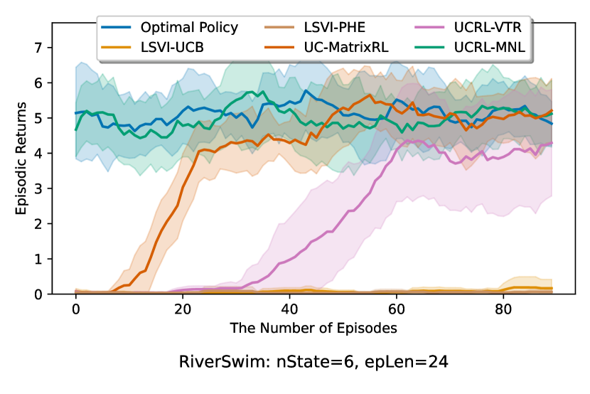
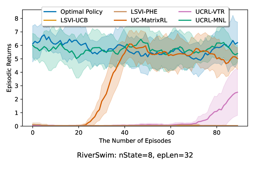
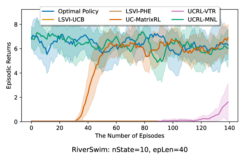
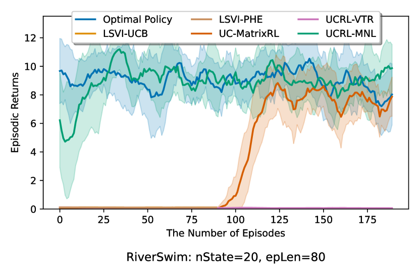
Figure 2: Episodic returns over 10 independent runs under the different RiverSwim environments

We perform a total of four experiments while increasing the number of states for RiverSwim. To set the hyper-parameters for each algorithm, we performed a grid search over certain ranges. In each experiment, we evaluated the algorithms on 10 independent instances to report the average performance. First, Figure 2 shows the episodic return of each algorithm over 10 independent runs. When the number of states is small (e.g., $|\mathcal{S}|=6$), it can be seen that not only our algorithm but also other model-based algorithms learn the optimal policy relatively well. However, our algorithm UCRL-MNL clearly outperforms the existing algorithms. As the number of states increases (e.g., $|\mathcal{S}|=20$), we observe that our algorithm reaches the optimal values remarkably quickly compared to the other algorithms, outperforming the existing algorithms by significant margins.

Table 1 shows the average cumulative reward over the episodes of each algorithm for 10 independent runs. The proposed algorithm has an average cumulative reward similar to that of the optimal policy across all problem settings. The results of these experiments provide the evidence for the practicality of our proposed model and proposed algorithm. For more detail, please refer to Appendix G.

	RiverSwim Environment
Methods	$|\mathcal{S}|=6,H=24$	$|\mathcal{S}|=8,H=32$	$|\mathcal{S}|=10,H=40$	$|\mathcal{S}|=20,H=80$
Optimal Policy	513.70 $\pm$ 39.67	576.50 $\pm$ 43.65	959.70 $\pm$ 57.97	1816.50 $\pm$ 79.89
UCRL-MNL	492.64 $\pm$ 32.23	562.83 $\pm$ 44.72	948.64 $\pm$ 74.47	1777.11 $\pm$ 99.23
UC-MatrixRL	372.47 $\pm$ 18.04	334.13 $\pm$ 21.74	632.62 $\pm$ 25.22	682.15 $\pm$ 64.41
UCRL-VTR	191.72 $\pm$ 68.47	41.50 $\pm$ 27.81	28.59 $\pm$ 19.61	15.76 $\pm$ 0.848
LSVI-UCB	7.52 $\pm$ 5.284	4.42 $\pm$ 2.053	5.54 $\pm$ 1.123	10.97 $\pm$ 1.813
LSVI-PHE	5.15 $\pm$ 1.506	5.41 $\pm$ 2.081	5.23 $\pm$ 0.097	10.17 $\pm$ 0.139

Table 1: Average returns over 10 independent runs in RiverSwim environments

5 Conclusion

In this work, we propose a new MNL transition model for RL with function approximation overcoming the limitation of the linear function approximation and a new algorithm, UCRL-MNL. We establish the theoretical performance bound on the proposed algorithm’s regret. To the best of our knowledge, this is not only the first model-based RL algorithm with multinomial logistic function approximation, but also our algorithm enjoys the provable efficiency as well as superior practical performances.

Appendix A Proof of Proposition 1 (The Limitation of Linear Transition Model)

We provide counter-examples as a proof of Proposition 1 both for the bilinear transition case and for the low-rank MDP case.

Case 1) Bilinear transition (Yang and Wang, 2020). In the bilinear transition model, the transition probability kernel is given by

$$\mathbb{P}(s^{\prime}\mid s,a)=\phi(s,a)^{\top}M^{*}\psi(s^{\prime})$$

where $\phi:{\mathcal{S}}\times\mathcal{A}\rightarrow\mathbb{R}^{d}$, $\psi:{\mathcal{S}}\rightarrow\mathbb{R}^{d^{\prime}}$ are known feature maps and $M^{*}$ is an unknown transition core matrix. Let an MDP with $|{\mathcal{S}}|=2$ and $|\mathcal{A}|=2$ be given. Also, let us given the features of state-action $\phi(s,a)\in\mathbb{R}^{2}$ and next state features $\psi(s^{\prime})\in\mathbb{R}$ as follows:

$$\Phi^{\top}:=[\phi(s_{1},a_{1})^{\top},\phi(s_{1},a_{2})^{\top},\phi(s_{2},a_{1})^{\top},\phi(s_{2},a_{2})^{\top}]^{\top}=\begin{bmatrix}1&1\\ 1&2\\ 3&1\\ 2&3\end{bmatrix}$$

$$\Psi:=[\psi(s_{1}),\psi(s_{2})]=[1,-2]\,.$$

Then for the true transition core matrix $M^{*}\in\mathbb{R}^{2\times 1}$, the element-wise sum across each row of $\Phi^{\top}M^{*}\Psi$ should be 1, because it is the transition matrix for the given MDP. On the other hand, if let $M^{*}=[x,y]^{\top}$, then, we have

$$\Phi^{\top}M^{*}\Psi=\begin{bmatrix}\mathbb{P}(s_{1}\mid s_{1},a_{1})&\mathbb{P}(s_{2}\mid s_{1},a_{1})\\ \mathbb{P}(s_{1}\mid s_{1},a_{2})&\mathbb{P}(s_{2}\mid s_{1},a_{2})\\ \mathbb{P}(s_{1}\mid s_{2},a_{1})&\mathbb{P}(s_{2}\mid s_{2},a_{1})\\ \mathbb{P}(s_{1}\mid s_{2},a_{2})&\mathbb{P}(s_{2}\mid s_{2},a_{2})\\ \end{bmatrix}=\begin{bmatrix}x+y&-2(x+y)\\ x+2y&-2(x+2y)\\ 3x+y&-2(3x+y)\\ 2x+3y&-2(2x+3y)\\ \end{bmatrix}\,.$$

Then by the property of the transition probability kernel, we have the following 4 equations:

$$-x-y=1\,,-x-2y=1\,,-3x-y=1\,,-2x-3y=1\,.$$

However, this system of linear equations is inconsistent since there are more equations to be satisfied than the number of unknown variables. Hence, in general, no bilinear transition model can induce a proper probability distribution over next states for an arbitrary set of state and action features.

Case 2) Low-rank MDP (Yang and Wang, 2019; Jin et al., 2020; Zanette et al., 2020) In the low-rank MDP, the transition probability is given by

$$\mathbb{P}(\cdot\mid s,a)=\langle\phi(s,a),\boldsymbol{\mu}^{*}\rangle$$

where $\phi:{\mathcal{S}}\times\mathcal{A}\rightarrow\mathbb{R}^{d}$ is a known feature map and $\boldsymbol{\mu}^{*}\in\mathbb{R}^{d\times|{\mathcal{S}}|}$ is an unknown (signed) measure over ${\mathcal{S}}$. Let a low-rank MDP with $|{\mathcal{S}}|=2$ and $|\mathcal{A}|=2$ be given. Suppose that the features of state-action $\phi(s,a)\in\mathbb{R}^{3}$ are given as follows:

$$\Phi^{\top}:=[\phi(s_{1},a_{1})^{\top},\phi(s_{1},a_{2})^{\top},\phi(s_{2},a_{1})^{\top},\phi(s_{2},a_{2})^{\top}]^{\top}=\begin{bmatrix}1&1&1\\ 1&2&0\\ 3&1&4\\ 2&3&7\end{bmatrix}$$

Then similarly with the Case 1, the element-wise sum across each row of $\Phi^{\top}\boldsymbol{\mu}^{*}$ should be 1. If we let $\boldsymbol{\mu}^{*}$ as follows:

$$\boldsymbol{\mu}^{*}=\begin{bmatrix}x_{11}&x_{12}\\ x_{21}&x_{22}\\ x_{31}&x_{32}\\ \end{bmatrix}\,,$$

then, we have

$$\Phi^{\top}\boldsymbol{\mu}^{*}=\begin{bmatrix}\mathbb{P}(s_{1}\mid s_{1},a_{1})&\mathbb{P}(s_{2}\mid s_{1},a_{1})\\ \mathbb{P}(s_{1}\mid s_{1},a_{2})&\mathbb{P}(s_{2}\mid s_{1},a_{2})\\ \mathbb{P}(s_{1}\mid s_{2},a_{1})&\mathbb{P}(s_{2}\mid s_{2},a_{1})\\ \mathbb{P}(s_{1}\mid s_{2},a_{2})&\mathbb{P}(s_{2}\mid s_{2},a_{2})\\ \end{bmatrix}=\begin{bmatrix}x_{11}+x_{21}+x_{31}&x_{12}+x_{22}+x_{32}\\ x_{11}+2x_{21}&x_{12}+2x_{22}\\ 3x_{11}+x_{21}+4x_{31}&3x_{12}+x_{22}+4x_{32}\\ 2x_{11}+3x_{21}+7x_{31}&2x_{12}+3x_{22}+7x_{32}\\ \end{bmatrix}\,.$$

Then by the property of the transition probability kernel, we have the following 4 equations:

$$x_{11}+x_{12}+x_{21}+x_{22}+x_{31}+x_{32}=1\,,$$

$$x_{11}+x_{12}+2x_{21}+2x_{22}=1\,,$$

$$3x_{11}+3x_{12}+x_{21}+x_{22}+4x_{31}+4x_{32}=1\,,$$

$$2x_{11}+2x_{12}+3x_{21}+3x_{22}+7x_{31}+7x_{32}=1\,.$$

On the other hand, if we put

$$Q=\begin{bmatrix}1&1&1&1&1&1\\ 1&1&2&2&0&0\\ 3&3&1&1&4&4\\ 2&2&3&3&7&7\\ \end{bmatrix}\text{ and }b=\begin{bmatrix}1\\ 1\\ 1\\ 1\\ \end{bmatrix}\,$$

then we have $\operatorname{rank}[Q\mid b]=4$ and $\operatorname{rank}Q=3$. Since the rank of the augmented matrix $[Q\mid b]$ is greater than the rank of the coefficient matrix $Q$, by the Rouché-Capelli theorem (Shafarevich and Remizov, 2012), the system of linear equations is inconsistent. Hence, in general, no transition model for a low-rank MDP can induce a proper probability distribution over next states for an arbitrary set of state and action features.

Appendix B Proof of Proposition 2

For the analysis of regret bound in (Yang and Wang, 2020), the authors impose regularity assumptions on features. In particular, they define $\Psi=[\psi(s_{1}),\ldots,\psi(s_{|\mathcal{S}|})]^{\top}\in\mathbb{R}^{|\mathcal{S}|\times d^{\prime}}$ as the matrix of all features $\psi$ of next states and assume $\Psi$ can satisfy $\|\Psi^{\top}v\|_{\infty}\leq C_{\psi}\|v\|_{\infty}$ for some universal constant $C_{\psi}>0$ and for any $v\in\mathbb{R}^{|\mathcal{S}|}$. However, each component of $\Psi^{\top}v$ consists of the sum of a total of $|\mathcal{S}|$ elements, thus the upper bound of $\|\Psi^{\top}v\|_{\infty}$ should depend on $|{\mathcal{S}}|$, i.e., $\|\Psi^{\top}v\|_{\infty}\leq C_{\psi}|\mathcal{S}|\|v\|_{\infty}$. Hence, the regret bound in (Yang and Wang, 2020) would increase by a factor of $|\mathcal{S}|$.

Appendix C Analyses and Proofs for Theorem 1

In this section, we establish all the necessary analyses of lemmas for proving Theorem 1. Also, we provide the proof of the Theorem 1 at the end of this section.

First, we define the high probability event for the concentration of the MLE.

Definition 2 (Good event)

Define the following event:

$$\mathcal{E}_{k}(\delta)=\left\{\|\hat{\theta}_{k^{\prime}}-\theta^{*}\|_{A_{k^{\prime}}}\leq\beta_{k^{\prime}}(\delta),\forall k^{\prime}\leq k\right\}\,.$$

Note that by Lemma 1, for any given $\delta\in(0,1)$, we can say that the event $\mathcal{E}_{K}(\delta^{\prime})$ happens with probability at least $1-\delta$, where $\delta^{\prime}=\delta/K$

Remark 1

Without loss of generality, we may assume that for a fixed $s^{\prime}\in{\mathcal{S}}$ we can have $\varphi(s,a,s^{\prime})={\bf 0}$. This is because suppose that a feature map $\phi(s,a,s^{\prime})\in\mathbb{R}^{d}$ is given and the transition probability is given by (1) using the feature map $\phi$, i.e., $P(s^{\prime}\mid s,a)=\frac{\exp(\phi(s,a,s^{\prime})^{\top}\theta^{*})}{\sum_{\widetilde{s}\in\mathcal{S}_{s,a}}\exp(\phi(s,a,\widetilde{s})^{\top}\theta^{*})}$. Then, for a fixed state $s^{\prime}\in\mathcal{S}_{s,a}$, by dividing the denominator and numerator by $\exp(\phi(s,a,s^{\prime})^{\top}\theta^{*})$, and by defining $\varphi(s,a,\widetilde{s}):=\phi(s,a,\widetilde{s})-\phi(s,a,s^{\prime})$ we have a well-defined feature map $\varphi$ which induces a consistent transition probability defined by $\phi$, but $\varphi(s,a,s^{\prime})={\bf 0}$.

C.1 Proof of Lemma 1

Proof [Proof of Lemma 1]

Let us define the function $G_{k}(\theta)$ as the difference in the gradients of the ridge penalized maximum likelihood in Eq.(3):

$$G_{k}(\theta):=\sum_{\begin{subarray}{c}k^{\prime}<k,\\ h\leq H\end{subarray}}\sum_{s^{\prime}\in\mathcal{S}_{k^{\prime},h}}[p_{k^{\prime},h}(s^{\prime},\theta)-p_{k^{\prime},h}(s^{\prime},\theta^{*})]\varphi_{k^{\prime},h,s^{\prime}}+\lambda(\theta-\theta^{*})\,.$$

Then, it follows that

$$G_{k}(\hat{\theta}_{k}) =\sum_{\begin{subarray}{c}k^{\prime}<k,\\ h\leq H\end{subarray}}\sum_{s^{\prime}\in\mathcal{S}_{k^{\prime},h}}[p_{k^{\prime},h}(s^{\prime},\hat{\theta}_{k})-p_{k^{\prime},h}(s^{\prime},\theta^{*})]\varphi_{k^{\prime},h,s^{\prime}}+\lambda(\hat{\theta}_{k}-\theta^{*})$$

$$=\sum_{\begin{subarray}{c}k^{\prime}<k,\\ h\leq H\end{subarray}}\!\sum_{s^{\prime}\in\mathcal{S}_{k^{\prime},h}}\!\!\![p_{k^{\prime},h}(s^{\prime},\hat{\theta}_{k})-y_{k^{\prime},h}^{s^{\prime}}]\varphi_{k^{\prime},h,s^{\prime}}+\lambda\hat{\theta}_{k}+\!\!\sum_{\begin{subarray}{c}k^{\prime}<k,\\ h\leq H\end{subarray}}\!\sum_{s^{\prime}\in\mathcal{S}_{k^{\prime},h}}\!\!\![y_{k^{\prime},h}^{s^{\prime}}-p_{k^{\prime},h}(s^{\prime},\theta^{*})]\varphi_{k^{\prime},h,s^{\prime}}-\lambda\theta^{*}$$

$$={\bf 0}+\sum_{\begin{subarray}{c}k^{\prime}<k,\\ h\leq H\end{subarray}}\sum_{s^{\prime}\in\mathcal{S}_{k^{\prime},h}}\epsilon_{k^{\prime},h}^{s^{\prime}}\varphi_{k^{\prime},h,s^{\prime}}-\lambda\theta^{*}$$

where $\epsilon_{k^{\prime},h}^{s^{\prime}}:=y_{k^{\prime},h}^{s^{\prime}}-p_{k^{\prime},h}(s^{\prime},\theta^{*})$ and the second equality holds since $\hat{\theta}_{k}$ is the maximizer of Eq.(3), which means $\hat{\theta}_{k}$ is the solution of the following equation:

$$\sum_{\begin{subarray}{c}k^{\prime}<k,\\ h\leq H\end{subarray}}\sum_{s^{\prime}\in\mathcal{S}_{k^{\prime},h}}[p_{k^{\prime},h}(s^{\prime},\hat{\theta}_{k})-y_{k^{\prime},h}^{s^{\prime}}]\varphi_{k^{\prime},h,s^{\prime}}+\lambda\hat{\theta}_{k}={\bf 0}$$

On the other hand, by Remark 1, if we denote a state in the set of reachable states $\mathcal{S}_{k^{\prime},h}$ satisfying $\varphi(s,a,s^{\prime})={\bf 0}$ as $\dot{s}_{k^{\prime},h}$, then we have

$$p_{k^{\prime},h}(s^{\prime},\theta) =\frac{\exp(\varphi_{k^{\prime},h,s^{\prime}}^{\top}\theta)}{\sum_{s^{\prime\prime}\in\mathcal{S}_{k^{\prime},h}}\exp(\varphi_{k^{\prime},h,s^{\prime\prime}}^{\top}\theta)}$$

$$=\frac{\exp(\varphi_{k^{\prime},h,s^{\prime}}^{\top}\theta)}{1+\sum_{s^{\prime\prime}\in\mathcal{S}_{k^{\prime},h}\backslash\{\dot{s}_{k^{\prime},h}\}}\exp(\varphi_{k^{\prime},h,s^{\prime\prime}}^{\top}\theta)}\,.$$

Notice that for $j\in[d]$, we have

$$\frac{\partial{p_{k^{\prime},h}(s^{\prime},\theta)}}{\partial{\theta_{j}}}$$

$$=\frac{\exp(\varphi_{k^{\prime},h,s^{\prime}}^{\top}\theta)\varphi_{k^{\prime},h,s^{\prime}}^{(j)}\left(1+\!\!\!\!\!\!\displaystyle\sum_{s^{\prime\prime}\in\mathcal{S}_{k^{\prime},h}\backslash\{\dot{s}_{k^{\prime},h}\}}\!\!\!\!\!\!\exp(\varphi_{k^{\prime},h,s^{\prime\prime}}^{\top}\theta)\right)-\exp(\varphi_{k^{\prime},h,s^{\prime}}^{\top}\theta)\left(\displaystyle\sum_{s^{\prime\prime}\in\mathcal{S}_{k^{\prime},h}\backslash\{\dot{s}_{k^{\prime},h}\}}\!\!\!\!\!\!\exp(\varphi_{k^{\prime},h,s^{\prime\prime}}^{\top}\theta)\varphi_{k^{\prime},h,s^{\prime\prime}}^{(j)}\right)}{\left(1+\!\!\!\!\!\!\displaystyle\sum_{s^{\prime\prime}\in\mathcal{S}_{k^{\prime},h}\backslash\{\dot{s}_{k^{\prime},h}\}}\exp(\varphi_{k^{\prime},h,s^{\prime\prime}}^{\top}\theta)\right)^{2}}$$

$$=p_{k^{\prime},h}(s^{\prime},\theta)\varphi_{k^{\prime},h,s^{\prime}}^{(j)}-p_{k^{\prime},h}(s^{\prime},\theta)\sum_{s^{\prime\prime}\in\mathcal{S}_{k^{\prime},h}\backslash\{\dot{s}_{k^{\prime},h}\}}p_{k^{\prime},h}(s^{\prime\prime},\theta)\varphi_{k^{\prime},h,s^{\prime\prime}}^{(j)}\,.$$

Then, we have

$$\nabla_{\theta}p_{k^{\prime},h}(s^{\prime},\theta)=p_{k^{\prime},h}(s^{\prime},\theta)\varphi_{k^{\prime},h,s^{\prime}}-p_{k^{\prime},h}(s^{\prime},\theta)\sum_{s^{\prime\prime}\in\mathcal{S}_{k^{\prime},h}\backslash\{\dot{s}_{k^{\prime},h}\}}p_{k^{\prime},h}(s^{\prime\prime},\theta)\varphi_{k^{\prime},h,s^{\prime\prime}}\,.$$

Then for any $\theta_{1},\theta_{2}\in\mathbb{R}^{d}$, the mean value theorem implies that there exists $\bar{\theta}=\nu\theta_{1}+(1-\nu)\theta_{2}$ with some $\nu\in(0,1)$ such that

$$G_{k}(\theta_{1})-G_{k}(\theta_{2}) =\sum_{\begin{subarray}{c}k^{\prime}<k,\\ h\leq H\end{subarray}}\sum_{s^{\prime}\in\mathcal{S}_{k^{\prime},h}}[p_{k^{\prime},h}(s^{\prime},\theta_{1})-p_{k^{\prime},h}(s^{\prime},\theta_{2})]\varphi_{k^{\prime},h,s^{\prime}}+\lambda(\theta_{1}-\theta_{2})$$

$$=\sum_{\begin{subarray}{c}k^{\prime}<k,\\ h\leq H\end{subarray}}\sum_{s^{\prime}\in\mathcal{S}_{k^{\prime},h}}\left(\nabla_{\theta}p_{k^{\prime},h}(s^{\prime},\bar{\theta})\right)^{\top}(\theta_{1}-\theta_{2})\varphi_{k^{\prime},h,s^{\prime}}+\lambda(\theta_{1}-\theta_{2})$$

$$=\sum_{\begin{subarray}{c}k^{\prime}<k,\\ h\leq H\end{subarray}}\left[H_{k^{\prime}}+\lambda I_{d}\right](\theta_{1}-\theta_{2})$$

where $H_{k^{\prime}}$ is defined as follows:

$$H_{k^{\prime}}:=\sum_{s^{\prime}\in\mathcal{S}_{k^{\prime},h}}p_{k^{\prime},h}(s^{\prime},\theta)\varphi_{k^{\prime},h,s^{\prime}}\varphi_{k^{\prime},h,s^{\prime}}^{\top}-\sum_{s^{\prime}\in\mathcal{S}_{k^{\prime},h}}\sum_{s^{\prime\prime}\in\mathcal{S}_{k^{\prime},h}}p_{k^{\prime},h}(s^{\prime},\theta)p_{k^{\prime},h}(s^{\prime\prime},\theta)\varphi_{k^{\prime},h,s^{\prime}}\varphi_{k^{\prime},h,s^{\prime\prime}}^{\top}\,.$$

Also, to identify that $H_{k^{\prime}}$ is positive semi-definite, note that

$$(x-y)(x-y)^{\top}=xx^{\top}+yy^{\top}-xy^{\top}-yx^{\top}\succcurlyeq{\bf 0}$$

which implies $xx^{\top}+yy^{\top}\succcurlyeq xy^{\top}+yx^{\top}$ for any $x,y\in\mathbb{R}^{d}$. Therefore, it follows that

$$H_{k^{\prime}} =\sum_{s^{\prime}\in\mathcal{S}_{k^{\prime},h}}p_{k^{\prime},h}(s^{\prime},\theta)\varphi_{k^{\prime},h,s^{\prime}}\varphi_{k^{\prime},h,s^{\prime}}^{\top}-\sum_{s^{\prime}\in\mathcal{S}_{k^{\prime},h}}\sum_{s^{\prime\prime}\in\mathcal{S}_{k^{\prime},h}}p_{k^{\prime},h}(s^{\prime},\theta)p_{k^{\prime},h}(s^{\prime\prime},\theta)\varphi_{k^{\prime},h,s^{\prime}}\varphi_{k^{\prime},h,s^{\prime\prime}}^{\top}$$

$$=\sum_{s^{\prime}\in\mathcal{S}_{k^{\prime},h}}p_{k^{\prime},h}(s^{\prime},\theta)\varphi_{k^{\prime},h,s^{\prime}}\varphi_{k^{\prime},h,s^{\prime}}^{\top}$$

$$\phantom{{}={}}-\frac{1}{2}\sum_{s^{\prime}\in\mathcal{S}_{k^{\prime},h}}\sum_{s^{\prime\prime}\in\mathcal{S}_{k^{\prime},h}}p_{k^{\prime},h}(s^{\prime},\theta)p_{k^{\prime},h}(s^{\prime\prime},\theta)(\varphi_{k^{\prime},h,s^{\prime}}\varphi_{k^{\prime},h,s^{\prime\prime}}^{\top}+\varphi_{k^{\prime},h,s^{\prime\prime}}\varphi_{k^{\prime},h,s^{\prime}}^{\top})$$

$$\succcurlyeq\sum_{s^{\prime}\in\mathcal{S}_{k^{\prime},h}}p_{k^{\prime},h}(s^{\prime},\theta)\varphi_{k^{\prime},h,s^{\prime}}\varphi_{k^{\prime},h,s^{\prime}}^{\top}$$

$$\phantom{{}={}}-\frac{1}{2}\sum_{s^{\prime}\in\mathcal{S}_{k^{\prime},h}}\sum_{s^{\prime\prime}\in\mathcal{S}_{k^{\prime},h}}p_{k^{\prime},h}(s^{\prime},\theta)p_{k^{\prime},h}(s^{\prime\prime},\theta)(\varphi_{k^{\prime},h,s^{\prime}}\varphi_{k^{\prime},h,s^{\prime}}^{\top}+\varphi_{k^{\prime},h,s^{\prime\prime}}\varphi_{k^{\prime},h,s^{\prime\prime}}^{\top})$$

$$=\sum_{s^{\prime}\in\mathcal{S}_{k^{\prime},h}}p_{k^{\prime},h}(s^{\prime},\theta)\varphi_{k^{\prime},h,s^{\prime}}\varphi_{k^{\prime},h,s^{\prime}}^{\top}-\sum_{s^{\prime}\in\mathcal{S}_{k^{\prime},h}}\!\sum_{s^{\prime\prime}\in\mathcal{S}_{k^{\prime},h}}p_{k^{\prime},h}(s^{\prime},\theta)p_{k^{\prime},h}(s^{\prime\prime},\theta)\varphi_{k^{\prime},h,s^{\prime}}\varphi_{k^{\prime},h,s^{\prime}}^{\top}$$

Therefore, we have

$$H_{k^{\prime}} \succcurlyeq\sum_{s^{\prime}\in\mathcal{S}_{k^{\prime},h}\backslash\{\dot{s}_{k^{\prime},h}\}}p_{k^{\prime},h}(s^{\prime},\theta)\varphi_{k^{\prime},h,s^{\prime}}\varphi_{k^{\prime},h,s^{\prime}}^{\top}$$

$$\phantom{{}={}}-\sum_{s^{\prime}\in\mathcal{S}_{k^{\prime},h}\backslash\{\dot{s}_{k^{\prime},h}\}}\sum_{s^{\prime\prime}\in\mathcal{S}_{k^{\prime},h}\backslash\{\dot{s}_{k^{\prime},h}\}}p_{k^{\prime},h}(s^{\prime},\theta)p_{k^{\prime},h}(s^{\prime\prime},\theta)\varphi_{k^{\prime},h,s^{\prime}}\varphi_{k^{\prime},h,s^{\prime}}^{\top}$$

$$=\sum_{s^{\prime}\in\mathcal{S}_{k^{\prime},h}\backslash\{\dot{s}_{k^{\prime},h}\}}p_{k^{\prime},h}(s^{\prime},\theta)\left(1-\sum_{s^{\prime\prime}\in\mathcal{S}_{k^{\prime},h}\backslash\{\dot{s}_{k^{\prime},h}\}}p_{k^{\prime},h}(s^{\prime\prime},\theta)\right)\varphi_{k^{\prime},h,s^{\prime}}\varphi_{k^{\prime},h,s^{\prime}}^{\top}$$

$$=\sum_{s^{\prime}\in\mathcal{S}_{k^{\prime},h}\backslash\{\dot{s}_{k^{\prime},h}\}}p_{k^{\prime},h}(s^{\prime},\theta)p_{k^{\prime},h}(\dot{s}_{k^{\prime},h},\theta)\varphi_{k^{\prime},h,s^{\prime}}\varphi_{k^{\prime},h,s^{\prime}}^{\top}$$

$$\succcurlyeq\sum_{s^{\prime}\in\mathcal{S}_{k^{\prime},h}\backslash\{\dot{s}_{k^{\prime},h}\}}\kappa\varphi_{k^{\prime},h,s^{\prime}}\varphi_{k^{\prime},h,s^{\prime}}^{\top}$$

where the last inequality comes from the Assumption 3. Then for any $\theta_{1}\neq\theta_{2}$, we have

$$(\theta_{1}-\theta_{2})^{\top}(G_{k}(\theta_{1})-G_{k}(\theta_{2}))$$

$$=(\theta_{1}-\theta_{2})^{\top}\left(\sum_{\begin{subarray}{c}k^{\prime}<k,\\ h\leq H\end{subarray}}H_{k^{\prime}}+\lambda I_{d}\right)(\theta_{1}-\theta_{2})$$

$$\geq(\theta_{1}-\theta_{2})^{\top}\left(\sum_{\begin{subarray}{c}k^{\prime}<k,\\ h\leq H\end{subarray}}\sum_{s^{\prime}\in\mathcal{S}_{k^{\prime},h}\backslash\{\dot{s}_{k^{\prime},h}\}}\kappa\varphi_{k^{\prime},h,s^{\prime}}\varphi_{k^{\prime},h,s^{\prime}}^{\top}+\lambda I_{d}\right)(\theta_{1}-\theta_{2})$$

$$=(\theta_{1}-\theta_{2})^{\top}\kappa\left(\sum_{\begin{subarray}{c}k^{\prime}<k,\\ h\leq H\end{subarray}}\sum_{s^{\prime}\in\mathcal{S}_{k^{\prime},h}\backslash\{\dot{s}_{k^{\prime},h}\}}\kappa\varphi_{k^{\prime},h,s^{\prime}}\varphi_{k^{\prime},h,s^{\prime}}^{\top}+\frac{\lambda}{\kappa}I_{d}\right)(\theta_{1}-\theta_{2})$$

$$\geq(\theta_{1}-\theta_{2})^{\top}(\kappa A_{k})(\theta_{1}-\theta_{2})$$

$$>0\,,$$

which means $G_{k}(\theta)$ is an injection from $\mathbb{R}^{d}$ to $\mathbb{R}^{d}$, and so $G^{-1}$ is well-defined. Hence, for any $\theta\in\mathbb{R}^{d}$, since $G_{k}(\theta^{*})={\bf 0}$, we have

$$\|G_{k}(\theta)\|_{A_{k}^{-1}}^{2} =\|G_{k}(\theta)-G_{k}(\theta^{*})\|_{A_{k}^{-1}}^{2}$$

$$=\left(G_{k}(\theta)-G_{k}(\theta^{*})\right)^{\top}A_{k}^{-1}\left(G_{k}(\theta)-G_{k}(\theta^{*})\right)$$

$$=(\theta-\theta^{*})^{\top}\left(\sum_{\begin{subarray}{c}k^{\prime}<k,\\ h\leq H\end{subarray}}H_{k^{\prime}}+\lambda I_{d}\right)A_{k}^{-1}\left(\sum_{\begin{subarray}{c}k^{\prime}<k,\\ h\leq H\end{subarray}}H_{k^{\prime}}+\lambda I_{d}\right)(\theta-\theta^{*})$$

$$\geq\kappa^{2}(\theta-\theta^{*})^{\top}A_{k}(\theta-\theta^{*})$$

$$=\kappa^{2}\|\theta-\theta^{*}\|_{A_{k}}^{2}$$

where the inequality follows from the fact:

$$\sum_{\begin{subarray}{c}k^{\prime}<k,\\ h\leq H\end{subarray}}H_{k^{\prime}}+\lambda I_{d}\succcurlyeq\kappa A_{k}\,.$$

Now, from the definition of $G_{k}(\hat{\theta}_{k})$, we have

$$\kappa\|\hat{\theta}_{k}-\theta^{*}\|_{A_{k}} \leq\|G_{k}(\hat{\theta}_{k})\|_{A_{k}^{-1}}$$

$$\leq\left\|\sum_{\begin{subarray}{c}k^{\prime}<k,\\ h\leq H\end{subarray}}\sum_{s^{\prime}\in\mathcal{S}_{k^{\prime},h}}\epsilon_{k^{\prime},h}^{s^{\prime}}\varphi_{k^{\prime},h,s^{\prime}}\right\|_{A_{k}^{-1}}+\lambda\|\theta^{*}\|_{A_{k}^{-1}}\,.$$

Then by Lemma 6, since the noise $\epsilon_{k^{\prime},h}^{s^{\prime}}$ is $1$-sub-Gaussian, we have

$$\left\|\sum_{\begin{subarray}{c}k^{\prime}<k,\\ h\leq H\end{subarray}}\sum_{s^{\prime}\in\mathcal{S}_{k^{\prime},h}}\epsilon_{k^{\prime},h}^{s^{\prime}}\varphi_{k^{\prime},h,s^{\prime}}\right\|^{2}_{A_{k}^{-1}}\leq 2\log\left(\frac{\det(A_{k})^{1/2}\det(\lambda I)^{-1/2}}{\delta}\right)$$

with probability at least $1-\delta$. Then by combining the result in Lemma 7, we have

$$\left\|\sum_{\begin{subarray}{c}k^{\prime}<k,\\ h\leq H\end{subarray}}\sum_{s^{\prime}\in\mathcal{S}_{k^{\prime},h}}\epsilon_{k^{\prime},h}^{s^{\prime}}\varphi_{k^{\prime},h,s^{\prime}}\right\|^{2}_{A_{k}^{-1}} \leq 2\left[\frac{d}{2}\log\left(\frac{\mathop{\mathrm{tr}}(\lambda I_{d})+kH\mathcal{U}}{d}\right)-\frac{1}{2}\log\det(\lambda I_{d})+\log\frac{1}{\delta}\right]$$

$$=2\left[\frac{d}{2}\log\left(\frac{d\lambda+kH\mathcal{U}}{d}\right)-\frac{1}{2}\log\lambda^{d}+\log\frac{1}{\delta}\right]$$

$$=d\log\left(1+\frac{kH\mathcal{U}}{d\lambda}\right)+2\log\frac{1}{\delta}\,.$$

On the other hand, for $\|\theta^{*}\|_{A_{k}^{-1}}$, we have

$$\|\theta^{*}\|_{A_{k}^{-1}}^{2}={\theta^{*}}^{\top}A_{k}^{-1}\theta^{*}\leq\frac{1}{\lambda}{\theta^{*}}^{\top}\theta^{*}=\frac{\|\theta^{*}\|_{2}^{2}}{\lambda}\,.$$

Hence, we have $\lambda\|\theta^{*}\|_{A_{k}^{-1}}\leq\sqrt{\lambda}L_{\theta}$. Then, by combining the results, we have that

$$\|\hat{\theta}_{k}-\theta^{*}\|_{A_{k}} \leq\underbrace{\frac{1}{\kappa}\sqrt{d\log\left(1+\frac{kH\mathcal{U}}{d\lambda}\right)+2\log\frac{1}{\delta}}+\frac{1}{\kappa}\sqrt{\lambda}L_{\theta}}_{\beta_{k}(\delta)}$$

with probability at least $1-\delta$.  

C.2 Proof of Lemma 2

Proof  We prove this by backwards induction on $h$. For the base case $h=H$, by definition of (4)

$$\hat{Q}_{k,H}(s,a)=r(s,a)=Q^{*}_{H}(s,a)$$

since $\hat{V}_{k,H+1}(s)=V^{*}_{H+1}(s)=0$ for all $s\in{\mathcal{S}}$. Suppose that the statement holds for step $h+1$ for some $1\leq h\leq H-1$. Then, for step $h$ and for all $(s,a)\in\mathcal{S}\times\mathcal{A}$,

$$\hat{Q}_{k,h}(s,a) =r(s,a)+\max_{\theta\in\mathcal{C}_{k}}\frac{\sum_{s^{\prime}\in\mathcal{S}_{s,a}}\exp(\varphi(s,a,s^{\prime})^{\top}\theta)\hat{V}_{k,h+1}(s^{\prime})}{\sum_{s^{\prime}\in\mathcal{S}_{s,a}}\exp(\varphi(s,a,s^{\prime})^{\top}\theta)}$$

$$\geq r(s,a)+\frac{\sum_{s^{\prime}\in\mathcal{S}_{s,a}}\exp(\varphi(s,a,s^{\prime})^{\top}\theta^{*})\hat{V}_{k,h+1}(s^{\prime})}{\sum_{s^{\prime}\in\mathcal{S}_{s,a}}\exp(\varphi(s,a,s^{\prime})^{\top}\theta^{*})}$$

$$=r(s,a)+P_{h}\hat{V}_{k,h+1}(s,a)$$

$$\geq r(s,a)+P_{h}V^{*}_{h+1}(s,a)$$

$$=Q^{*}_{h}(s,a)$$

where the first inequality holds by the construction of $\hat{Q}_{k,h}$, the second inequality follows from the induction hypothesis.  

C.3 Proof of Lemma 3

Proof  Let

$$\widetilde{\theta}:=\mathop{\mathrm{argmax}}_{\theta\in\mathcal{C}_{t}}\frac{\sum_{s^{\prime}\in\mathcal{S}_{k,h}}\exp(\varphi_{k,h,s^{\prime}}^{\top}\theta)\hat{V}_{k,h+1}(s^{\prime})}{\sum_{s^{\prime}\in\mathcal{S}_{k,h}}\exp(\varphi_{k,h,s^{\prime}}^{\top}\theta)}\,.$$

Then, we have

$$\hat{Q}_{k,h}(s_{k,h},a_{k,h})-\left[r(s_{k,h},a_{k,h})+P_{h}\hat{V}_{k,h+1}(s_{k,h},a_{k,h})\right]$$

$$=\frac{\sum_{s^{\prime}\in\mathcal{S}_{k,h}}\exp(\varphi_{k,h,s^{\prime}}^{\top}\widetilde{\theta})\hat{V}_{k,h+1}(s^{\prime})}{\sum_{s^{\prime}\in\mathcal{S}_{k,h}}\exp(\varphi_{k,h,s^{\prime}}^{\top}\widetilde{\theta})}-\frac{\sum_{s^{\prime}\in\mathcal{S}_{k,h}}\exp(\varphi_{k,h,s^{\prime}}^{\top}\theta^{*})\hat{V}_{k,h+1}(s^{\prime})}{\sum_{s^{\prime}\in\mathcal{S}_{k,h}}\exp(\varphi_{k,h,s^{\prime}}^{\top}\theta^{*})}\,.$$ (7)

Then by the mean value theorem, there exists $\bar{\theta}=\nu\widetilde{\theta}+(1-\nu)\theta^{*}$ for some $0\leq\nu\leq 1$ satisfying that

$$(\ref{eq:value f.t concen 1}) =\frac{\left(\sum_{s^{\prime}\in\mathcal{S}_{k,h}}\exp(\varphi_{k,h,s^{\prime}}^{\top}\bar{\theta})\hat{V}_{k,h+1}(s^{\prime})\varphi_{k,h,s^{\prime}}^{\top}(\widetilde{\theta}-\theta^{*})\right)\left(\sum_{s^{\prime}\in\mathcal{S}_{k,h}}\exp(\varphi_{k,h,s^{\prime}}^{\top}\bar{\theta})\right)}{\left(\sum_{s^{\prime}\in\mathcal{S}_{k,h}}\exp(\varphi_{k,h,s^{\prime}}^{\top}\bar{\theta})\right)^{2}}$$

$$\phantom{{}={}}-\frac{\left(\sum_{s^{\prime}\in\mathcal{S}_{k,h}}\exp(\varphi_{k,h,s^{\prime}}^{\top}\bar{\theta})\hat{V}_{k,h+1}(s^{\prime})\right)\left(\sum_{s^{\prime}\in\mathcal{S}_{k,h}}\exp(\varphi_{k,h,s^{\prime}}^{\top}\bar{\theta})\varphi_{k,h,s^{\prime}}^{\top}(\widetilde{\theta}-\theta^{*})\right)}{\left(\sum_{s^{\prime}\in\mathcal{S}_{k,h}}\exp(\varphi_{k,h,s^{\prime}}^{\top}\bar{\theta})\right)^{2}}$$

$$=\sum_{s^{\prime}\in\mathcal{S}_{k,h}}p_{k,h}(s^{\prime},\bar{\theta})\hat{V}_{k,h+1}(s^{\prime})\varphi_{k,h,s^{\prime}}^{\top}(\widetilde{\theta}-\theta^{*})$$

$$\phantom{{}={}}-\left(\frac{\sum_{s^{\prime}\in\mathcal{S}_{k,h}}\exp(\varphi_{k,h,s^{\prime}}^{\top}\bar{\theta})\hat{V}_{k,h+1}(s^{\prime})}{\sum_{s^{\prime}\in\mathcal{S}_{k,h}}\exp(\varphi_{k,h,s^{\prime}}^{\top}\bar{\theta})}\right)\sum_{s^{\prime}\in\mathcal{S}_{k,h}}p_{k,h}(s^{\prime},\bar{\theta})\varphi_{k,h,s^{\prime}}^{\top}(\widetilde{\theta}-\theta^{*})$$

$$=\sum_{s^{\prime}\in\mathcal{S}_{k,h}}\left(\hat{V}_{k,h+1}(s^{\prime})-\frac{\sum_{s^{\prime}\in\mathcal{S}_{k,h}}\exp(\varphi_{k,h,s^{\prime}}^{\top}\bar{\theta})\hat{V}_{k,h+1}(s^{\prime})}{\sum_{s^{\prime}\in\mathcal{S}_{k,h}}\exp(\varphi_{k,h,s^{\prime}}^{\top}\bar{\theta})}\right)p_{k,h}(s^{\prime},\bar{\theta})\varphi_{k,h,s^{\prime}}^{\top}(\widetilde{\theta}-\theta^{*})$$

$$\leq H\sum_{s^{\prime}\in\mathcal{S}_{k,h}}p_{k,h}(s^{\prime},\bar{\theta})\varphi_{k,h,s^{\prime}}^{\top}(\widetilde{\theta}-\theta^{*})$$

$$\leq H\max_{s^{\prime}\in\mathcal{S}_{k,h}}|\varphi_{k,h,s^{\prime}}^{\top}(\widetilde{\theta}-\theta^{*})|$$

$$\leq H\max_{s^{\prime}\in\mathcal{S}_{k,h}}\|\varphi_{k,h,s^{\prime}}\|_{A_{k}^{-1}}\|\widetilde{\theta}-\theta^{*}\|_{A_{k}}$$

$$\leq H\max_{s^{\prime}\in\mathcal{S}_{k,h}}\|\varphi_{k,h,s^{\prime}}\|_{A_{k}^{-1}}(\|\widetilde{\theta}-\hat{\theta}_{k}\|_{A_{k}}+\|\hat{\theta}_{k}-\theta^{*}\|_{A_{k}})$$

$$\leq 2H\beta_{k}(\delta)\max_{s^{\prime}\in\mathcal{S}_{k,h}}\|\varphi_{k,h,s^{\prime}}\|_{A_{k}^{-1}}\,.$$

where the second inequality holds due to the definition of $p_{k,h}(s^{\prime},\bar{\theta})$.  

C.4 Proof of Theorem 1

Now we are ready to provide the proof of Theorem 1.

Proof [Proof of Theorem 1] By the condition of $\lambda$, we can guarantee that $\|\varphi_{k,h,s^{\prime}}\|_{A_{k}^{-1}}$ is smaller than 1 for all $k\in[K],h\in[H]$ and $s^{\prime}\in\mathcal{S}_{k,h}$, which means,

$$\|\varphi_{k,h,s^{\prime}}\|^{2}_{A_{k}^{-1}}=\varphi_{k,h,s^{\prime}}^{\top}A_{k}^{-1}\varphi_{k,h,s^{\prime}}\leq\frac{1}{\lambda}\|\varphi_{k,h,s^{\prime}}\|_{2}^{2}\leq\frac{1}{\lambda}L_{\varphi}^{2}\leq 1\,.$$

Let $\delta^{\prime}=\delta/2$. Then by Lemma 4, with probability at least $1-\delta/2$, we have

$$\textbf{Regret}_{\pi}(T) \leq 2H\beta_{K}(\delta^{\prime})\sqrt{KH\sum_{k=1}^{K}\sum_{h=1}^{H}\max_{s^{\prime}\in\mathcal{S}_{k,h}}\|\varphi_{k,h,s^{\prime}}\|_{A_{k}^{-1}}^{2}}+\sum_{k=1}^{K}\sum_{h=1}^{H}\dot{\zeta}_{k,h}$$

$$\leq 2H\beta_{K}(\delta^{\prime})\sqrt{2THd\log\left(1+\frac{KH\mathcal{U}}{d\lambda}\right)}+\sum_{k=1}^{K}\sum_{h=1}^{H}\dot{\zeta}_{k,h}\,,$$

where the second inequality follows from the Lemma 5. On the other hand, note that $\dot{\zeta}_{k,h}$ is a martingale difference satisfying $|\dot{\zeta}_{k,h}|\leq 2H$ and $\mathbb{E}[\dot{\zeta}_{k,h}\mid\mathcal{F}_{k,h}]=0$ where $\mathcal{F}_{k,h}:=\{s_{k^{\prime},h},a_{k^{\prime},h},y_{k^{\prime},h}:k^{\prime}<k,h\leq H\}\cup\{s_{k,h^{\prime}},a_{k,h^{\prime}},y_{k,h^{\prime}-1}:h^{\prime}\leq h\}$. By applying Azuma-Hoeffiding inequality, with probability at least $1-\delta/2$, we have

$$\sum_{k=1}^{K}\sum_{h=1}^{H}\dot{\zeta}_{k,h}\leq H\sqrt{2T\log(2/\delta)}\,.$$

By taking union bound, with probability at least $1-\delta$, we get the desired result as follows:

$$\textbf{Regret}_{\pi}(T)=\widetilde{\mathcal{O}}\left(\kappa^{-1}d\sqrt{H^{3}T}+H\sqrt{T}\right)\,.$$

 

Appendix D Supporting lemmas

In this section, we provide some supporting lemmas to be used in Appendix C.

Lemma 4

Let $\delta\in(0,1)$ be given. Conditioned on the event $\mathcal{E}_{K}(\delta)$, we have

$$\textbf{Regret}_{\pi}(T)\leq 2H\beta_{K}(\delta)\sqrt{KH\sum_{k=1}^{K}\sum_{h=1}^{H}\max_{s^{\prime}\in\mathcal{S}_{k,h}}\|\varphi_{k,h,s^{\prime}}\|_{A_{k}^{-1}}^{2}}+\sum_{k=1}^{K}\sum_{h=1}^{H}\dot{\zeta}_{k,h}\,,$$

where $\dot{\zeta}_{k,h}=\mathbb{E}_{s^{\prime}|s_{k,h},a_{k,h}}\Big{[}\left(\hat{V}_{k,h+1}-V^{\pi_{k}}_{h+1}\right)(s^{\prime})\Big{]}-\left(\hat{V}_{k,h+1}-V^{\pi_{k}}_{h+1}\right)(s_{k,h+1})$.

Proof [Proof of Lemma 4] Recall that

$$\textbf{Regret}_{\pi}(K)=\sum_{k=1}^{K}(V^{*}_{1}-V^{\pi_{k}}_{1})(s_{k,1})\,.$$

Conditioned on the event $\mathcal{E}_{K}(\delta)$, by Lemma 2, we have

$$(V^{*}_{1}-V^{\pi_{k}}_{1})(s_{k,1}) =(Q^{*}_{1}(s_{k,1},\pi^{*}(s_{k,1}))-V^{\pi_{k}}_{1}(s_{k,1}))$$

$$\leq(\hat{Q}_{k,1}(s_{k,1},\pi^{*}(s_{k,1}))-V^{\pi_{k}}_{1}(s_{k,1}))$$

$$\leq(\hat{Q}_{k,1}(s_{k,1},a_{k,1})-V^{\pi_{k}}_{1}(s_{k,1}))\,.$$

On the other hand, by Lemma 3, we have

$$\hat{Q}_{k,h}(s_{k,h},a_{k,h})\leq 2H\beta_{k}(\delta)\max_{s^{\prime}\in\mathcal{S}_{k,h}}\|\varphi_{k,h,s^{\prime}}\|_{A_{k}^{-1}}+\left[r(s_{k,h},a_{k,h})+P_{h}\hat{V}_{k,h+1}(s_{k,h},a_{k,h})\right]\,.$$

Then we have

$$\hat{Q}_{k,1}(s_{k,1},a_{k,1})-V^{\pi_{k}}_{1}(s_{k,1}) =\hat{Q}_{k,1}(s_{k,1},a_{k,1})-Q^{\pi_{k}}_{1}(s_{k,1},a_{k,1})$$

$$\leq 2H\beta_{k}(\delta)\max_{s^{\prime}\in\mathcal{S}_{k,1}}\|\varphi_{k,1,s^{\prime}}\|_{A_{k}^{-1}}+P_{1}(\hat{V}_{k,2}-V^{\pi_{k}}_{2})(s_{k,1},a_{k,1})$$

$$=2H\beta_{k}(\delta)\max_{s^{\prime}\in\mathcal{S}_{k,1}}\|\varphi_{k,1,s^{\prime}}\|_{A_{k}^{-1}}+\underbrace{\mathbb{E}_{s^{\prime}|s_{k,1},a_{k,1}}\Big{[}\left(\hat{V}_{k,2}-V^{\pi_{k}}_{2}\right)(s^{\prime})\Big{]}}_{\dot{\zeta}_{k,1}+\left(\hat{V}_{k,2}-V^{\pi_{k}}_{2}\right)(s_{k,2})}$$

$$=2H\beta_{k}(\delta)\max_{s^{\prime}\in\mathcal{S}_{k,1}}\|\varphi_{k,1,s^{\prime}}\|_{A_{k}^{-1}}+\left(\hat{V}_{k,2}-V^{\pi_{k}}_{2}\right)(s_{k,2})+\dot{\zeta}_{k,1}$$

where the inequality comes from the Lemma 3. Applying this logic recursively, we have

$$\hat{Q}_{k,1}(s_{k,1},a_{k,1})-V^{\pi_{k}}_{1}(s_{k,1}) \leq\sum_{h=1}^{H}2H\beta_{k}(\delta)\max_{s^{\prime}\in\mathcal{S}_{k,h}}\|\varphi_{k,h,s^{\prime}}\|_{A_{k}^{-1}}+\sum_{h=1}^{H}\dot{\zeta}_{k,h}$$

where $\dot{\zeta}_{k,h}=\mathbb{E}_{s^{\prime}|s_{k,h},a_{k,h}}\Big{[}\left(\hat{V}_{k,h+1}-V^{\pi_{k}}_{h+1}\right)(s^{\prime})\Big{]}-\left(\hat{V}_{k,h+1}-V^{\pi_{k}}_{h+1}\right)(s_{k,h+1})$.

By summing up, we get the desired result.

$$\textbf{Regret}_{\pi}(K) =\sum_{k=1}^{K}(V^{*}_{1}-V^{\pi_{k}}_{1})(s_{k,1})$$

$$\leq 2H\beta_{K}(\delta)\sum_{k=1}^{K}\sum_{h=1}^{H}\max_{s^{\prime}\in\mathcal{S}_{k,h}}\|\varphi_{k,h,s^{\prime}}\|_{A_{k}^{-1}}+\sum_{k=1}^{K}\sum_{h=1}^{H}\dot{\zeta}_{k,h}$$

$$\leq 2H\beta_{K}(\delta)\sqrt{KH\sum_{k=1}^{K}\sum_{h=1}^{H}\max_{s^{\prime}\in\mathcal{S}_{k,h}}\|\varphi_{k,h,s^{\prime}}\|_{A_{k}^{-1}}^{2}}+\sum_{k=1}^{K}\sum_{h=1}^{H}\dot{\zeta}_{k,h}\,.$$

 

Lemma 5

Define $A_{k}=\lambda I_{d}+\sum_{\begin{subarray}{c}k^{\prime}<k\\ h\leq H\end{subarray}}\sum_{s^{\prime}\in\mathcal{S}_{k^{\prime},h}}\!\varphi_{k^{\prime},h,s^{\prime}}\varphi_{k^{\prime},h,s^{\prime}}^{\top}$. If $\lambda\geq L_{\varphi}^{2}$, then

$$\sum_{\begin{subarray}{c}k^{\prime}<k\\ h\leq H\end{subarray}}\max_{s^{\prime}\in\mathcal{S}_{k^{\prime},h}}\|\varphi_{k^{\prime},h,s^{\prime}}\|_{A_{k}^{-1}}^{2}\leq 2Hd\log\left(1+\frac{kH\mathcal{U}}{d\lambda}\right)\,.$$

Proof  Recall that

$$A_{k+1}=A_{k}+\sum_{h\leq H}\sum_{s^{\prime}\in\mathcal{S}_{k,h}}\varphi_{k,h,s^{\prime}}\varphi_{k,h,s^{\prime}}^{\top}\,.$$

Since we have $A_{k}\succ{\bf 0}$, then we have

$$\det A_{k+1}=\det(A_{k})\det\left(I_{d}+A_{k}^{-1/2}\sum_{h=1}^{H}\sum_{s^{\prime}\in\mathcal{S}_{k,h}}\varphi_{k,h,s^{\prime}}\varphi_{k,h,s^{\prime}}^{\top}A_{k}^{-1/2}\right)\,.$$

Let $\lambda_{i}$ be an eigenvalue of $I_{d}+A_{k}^{-1/2}\sum_{h=1}^{H}\sum_{s^{\prime}\in\mathcal{S}_{k,h}}\varphi_{k,h,s^{\prime}}\varphi_{k,h,s^{\prime}}^{\top}A_{k}^{-1/2}$, $1\leq i\leq d$. Then, for all $1\leq i\leq d$, we have $\lambda_{i}\geq 1$ and

$$\sum_{i=1}^{d}(\lambda_{i}-1)=\mathop{\mathrm{tr}}\left(I_{d}+A_{k}^{-1/2}\sum_{h=1}^{H}\sum_{s^{\prime}\in\mathcal{S}_{k,h}}\varphi_{k,h,s^{\prime}}\varphi_{k,h,s^{\prime}}^{\top}A_{k}^{-1/2}\right)-d=\sum_{h=1}^{H}\sum_{s^{\prime}\in\mathcal{S}_{k,h}}\|\varphi_{k,h,s^{\prime}}\|_{A_{k}^{-1}}^{2}$$

Therefore, we have

$$\det\left(I_{d}+A_{k}^{-1/2}\sum_{h=1}^{H}\sum_{s^{\prime}\in\mathcal{S}_{k,h}}\varphi_{k,h,s^{\prime}}\varphi_{k,h,s^{\prime}}^{\top}A_{k}^{-1/2}\right) =\prod_{i=1}^{d}\lambda_{i}$$

$$=\prod_{i=1}^{d}\left[1+(\lambda_{i}-1)\right]$$

$$\geq 1+\sum_{i=1}^{d}(\lambda_{i}-1)$$

$$=1+\sum_{h=1}^{H}\sum_{s^{\prime}\in\mathcal{S}_{k,h}}\|\varphi_{k,h,s^{\prime}}\|_{A_{k}^{-1}}^{2}$$

$$\geq 1+\sum_{h=1}^{H}\max_{s^{\prime}\in\mathcal{S}_{k,h}}\|\varphi_{k,h,s^{\prime}}\|_{A_{k}^{-1}}^{2}$$

where the first inequality comes from the fact that $\left[1+(a-1)\right]\left[1+(b-1)\right]=1+(a-1)+(b-1)+(a-1)(b-1)\geq 1+(a-1)+(b-1)$ for some $a,b\geq 1$. On the other hand,

$$1+\sum_{h=1}^{H}\max_{s^{\prime}\in\mathcal{S}_{k,h}}\|\varphi_{k,h,s^{\prime}}\|_{A_{k}^{-1}}^{2} =\frac{\sum_{h=1}^{H}(1+H\max_{s^{\prime}\in\mathcal{S}_{k,h}}\|\varphi_{k,h,s^{\prime}}\|_{A_{k}^{-1}}^{2})}{H}$$

$$\geq\prod_{h=1}^{H}(1+H\max_{s^{\prime}\in\mathcal{S}_{k,h}}\|\varphi_{k,h,s^{\prime}}\|_{A_{k}^{-1}}^{2})^{1/H}$$

$$\geq\prod_{h=1}^{H}(1+\max_{s^{\prime}\in\mathcal{S}_{k,h}}\|\varphi_{k,h,s^{\prime}}\|_{A_{k}^{-1}}^{2})^{1/H}\,,$$

where the first inequality comes from the AM–GM inequality. Then, it follows that

$$\det A_{k+1} \geq\det(A_{k})\prod_{h=1}^{H}(1+\max_{s^{\prime}\in\mathcal{S}_{k,h}}\|\varphi_{k,h,s^{\prime}}\|_{A_{k}^{-1}}^{2})^{1/H}$$

$$\geq\det(\lambda I_{d})\prod_{k^{\prime}=1}^{k}\prod_{h=1}^{H}(1+\max_{s^{\prime}\in\mathcal{S}_{k^{\prime},h}}\|\varphi_{k^{\prime},h,s^{\prime}}\|_{A_{k^{\prime}}^{-1}}^{2})^{1/H}\,.$$

Since $\lambda\geq L_{\varphi}^{2}$, we have for all $k\in[K],h\in[H]$ and $s^{\prime}\in\mathcal{S}_{k,h}$

$$\|\varphi_{k,h,s^{\prime}}\|^{2}_{A_{k}^{-1}}=\varphi_{k,h,s^{\prime}}^{\top}A_{k}^{-1}\varphi_{k,h,s^{\prime}}\leq\frac{1}{\lambda}\|\varphi_{k,h,s^{\prime}}\|_{2}^{2}\leq\frac{1}{\lambda}L_{\varphi}^{2}\leq 1\,.$$

Then, using the fact that $z\leq 2\log(1+z)$ for any $z\in[0,1]$, we have

$$\sum_{\begin{subarray}{c}k^{\prime}<k\\ h\leq H\end{subarray}}\max_{s^{\prime}\in\mathcal{S}_{k^{\prime},h}}\|\varphi_{k^{\prime},h,s^{\prime}}\|_{A_{k^{\prime}}^{-1}}^{2} \leq 2\sum_{\begin{subarray}{c}k^{\prime}<k\\ h\leq H\end{subarray}}\log\left(1+\max_{s^{\prime}\in\mathcal{S}_{k^{\prime},h}}\|\varphi_{k^{\prime},h,s^{\prime}}\|_{A_{k^{\prime}}^{-1}}^{2}\right)$$

$$=2\log\prod_{k^{\prime}=1}^{k}\prod_{h=1}^{H}\left(1+\max_{s^{\prime}\in\mathcal{S}_{k^{\prime},h}}\|\varphi_{k^{\prime},h,s^{\prime}}\|_{A_{k^{\prime}}^{-1}}^{2}\right)$$

$$\leq 2H\log\left(\frac{\det A_{k+1}}{\det\lambda I_{d}}\right)$$

$$\leq 2H\log\left[\left(\frac{\mathop{\mathrm{tr}}(\lambda I_{d})+kH\mathcal{U}}{d}\right)^{d}\frac{1}{\det\lambda I_{d}}\right]$$

$$=2Hd\log\left(1+\frac{kH\mathcal{U}}{d\lambda}\right)\,,$$

where the last inequality follows from the Lemma 7.  

Appendix E Limitations

We assume a particular parametric model, the MNL model for the transition model of MDPs. Hence, realizability is assumed. Note that such realizability assumption is also imposed in almost all previous literature on provable reinforcement learning with function approximation (Yang and Wang, 2020; Jin et al., 2020; Zanette et al., 2020; Modi et al., 2020; Du et al., 2020; Cai et al., 2020; Ayoub et al., 2020; Wang et al., 2020; Weisz et al., 2021; He et al., 2021; Zhou et al., 2021a, b; Ishfaq et al., 2021). However, we hope that this condition can be relaxed in the future work.

Appendix F Additional Lemmas

Lemma 6 (Self-Normalized Inequality (Abbasi-Yadkori et al., 2011))

Let $\{\mathcal{F}_{t}\}_{t=0}^{\infty}$ be a filtration and $\{\eta_{t}\}_{t=1}^{\infty}$ be a real-valued stochastic process such that $\eta_{t}$ is $\mathcal{F}_{t}$-measurable and $\eta_{t}$ is conditionally $R$-sub-Gaussian for some $R\geq 0$. Let $\{x_{t}\}_{t=1}^{\infty}$ be an $\mathbb{R}^{d}$-valued stochastic process such that $x_{t}$ is $\mathcal{F}_{t-1}$-measurable. Assume that $V$ is a $d\times d$ positive definite matrix. For any $t\geq 0$, define $V_{t}:=V+\sum_{s=1}^{t}x_{s}x_{s}^{\top}$ and $S_{t}=\sum_{s=1}^{t}\eta_{s}x_{s}$. Then for any $\delta>0$, with probability at least $1-\delta$, for all $t\geq 0$, we have

$$\|S_{t}\|_{V_{t}^{-1}}^{2}\leq 2R^{2}\log\left(\frac{\det(V_{t})^{1/2}\det(V)^{-1/2}}{\delta}\right)\,.$$

Lemma 7 (Determinant-Trace Inequality (Abbasi-Yadkori et al., 2011))

Suppose $\|\varphi_{k^{\prime},h,s^{\prime}}\|_{2}\leq 1$ for all $k^{\prime}\leq k,h\leq H$, and $s^{\prime}\in\mathcal{S}_{k^{\prime},h}$. Then $\det(A_{k})$ is increasing with respect to $k$ and

$$\det(A_{k})\leq\left(\frac{\mathop{\mathrm{tr}}(\lambda I_{d})+kH\mathcal{U}}{d}\right)^{d}\,.$$

Lemma 8 (Lemma 8 in (Oh and Iyengar, 2019))

Suppose $\|\varphi_{k^{\prime},h,s^{\prime}}\|_{2}\leq 1$ for all $k^{\prime}\leq k,h\leq H$, and $s^{\prime}\in\mathcal{S}_{k^{\prime},h}$. Define $A_{k}=\lambda I_{d}+\sum_{\begin{subarray}{c}k^{\prime}<k\\ h\leq H\end{subarray}}\sum_{s^{\prime}\in\mathcal{S}_{k^{\prime},h}}\!\varphi_{k^{\prime},h,s^{\prime}}\varphi_{k^{\prime},h,s^{\prime}}^{\top}$. If $\lambda\geq L_{\varphi}^{2}$, then

$$\sum_{\begin{subarray}{c}k^{\prime}<k\\ h\leq H\end{subarray}}\max_{s^{\prime}\in\mathcal{S}_{k^{\prime},h}}\|\varphi_{k^{\prime},h,s^{\prime}}\|_{A_{k^{\prime}}^{-1}}^{2}\leq 2\log\left(\frac{\det A_{k}}{\lambda^{d}}\right)\,.$$ (8)

Appendix G Experiment Details

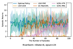
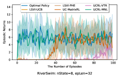
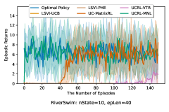
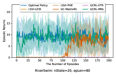
Figure 3: Episodic returns over 10 independent runs under the different RiverSwim environments (without smoothing effect)

In this section, we will explain the result for the RiverSwim in more detail. In Figure 2, the smoothing effect was applied for the sake of clear visualization of overall tendency. However, such smoothing may overshadow the performance of our algorithm in the early episodes — since it can make the results seem as if our proposed algorithm reached the optimal policy from the beginning. The episodic return without smoothing effect is presented in Figure 3. As can be seen in Figure 3, our proposed algorithm converges to the optimal policy within a few episodes. Compared to the benchmark algorithms, the reason why our proposed algorithm is able to converge quickly is that at every time step, other algorithms use only one feedback about the state where the actual transition occurred, whereas the proposed algorithm uses information of reachable states including the state in which no actual transition is occurred. This means that the proposed algorithm can get more information from one sample. Also, if the size of the set of reachable states is properly bounded (Note that $\mathcal{U}=3$ in this experiment) even when the size of the state space grows, we can see that our proposed algorithm has superior performance consistently, independent of the size of the state space.

References

- Abbasi-Yadkori et al. (2011) Y. Abbasi-Yadkori, D. Pál, and C. Szepesvári. Improved algorithms for linear stochastic bandits. Advances in neural information processing systems, 24:2312–2320, 2011.
- Abeille and Lazaric (2017) M. Abeille and A. Lazaric. Linear Thompson Sampling Revisited. In A. Singh and J. Zhu, editors, Proceedings of the 20th International Conference on Artificial Intelligence and Statistics, volume 54 of Proceedings of Machine Learning Research, pages 176–184. PMLR, 20–22 Apr 2017.
- Agrawal and Goyal (2013) S. Agrawal and N. Goyal. Thompson sampling for contextual bandits with linear payoffs. In International Conference on Machine Learning, pages 127–135. PMLR, 2013.
- Agrawal and Jia (2017) S. Agrawal and R. Jia. Posterior sampling for reinforcement learning: worst-case regret bounds. In Advances in Neural Information Processing Systems, pages 1184–1194, 2017.
- Auer (2002) P. Auer. Using confidence bounds for exploitation-exploration trade-offs. Journal of Machine Learning Research, 3(Nov):397–422, 2002.
- Auer et al. (2002) P. Auer, N. Cesa-Bianchi, and P. Fischer. Finite-time analysis of the multiarmed bandit problem. Machine learning, 47(2):235–256, 2002.
- Ayoub et al. (2020) A. Ayoub, Z. Jia, C. Szepesvari, M. Wang, and L. Yang. Model-based reinforcement learning with value-targeted regression. In International Conference on Machine Learning, pages 463–474. PMLR, 2020.
- Azar et al. (2017) M. G. Azar, I. Osband, and R. Munos. Minimax regret bounds for reinforcement learning. In International Conference on Machine Learning, pages 263–272. PMLR, 2017.
- Bradtke and Barto (1996) S. J. Bradtke and A. G. Barto. Linear least-squares algorithms for temporal difference learning. Machine learning, 22(1):33–57, 1996.
- Cai et al. (2020) Q. Cai, Z. Yang, C. Jin, and Z. Wang. Provably efficient exploration in policy optimization. In International Conference on Machine Learning, pages 1283–1294. PMLR, 2020.
- Chu et al. (2011) W. Chu, L. Li, L. Reyzin, and R. Schapire. Contextual bandits with linear payoff functions. In Proceedings of the Fourteenth International Conference on Artificial Intelligence and Statistics, pages 208–214. JMLR Workshop and Conference Proceedings, 2011.
- Dani et al. (2008) V. Dani, T. P. Hayes, and S. M. Kakade. Stochastic linear optimization under bandit feedback. 2008.
- Dann et al. (2017) C. Dann, T. Lattimore, and E. Brunskill. Unifying pac and regret: Uniform pac bounds for episodic reinforcement learning. In Advances in Neural Information Processing Systems, volume 30, pages 5713–5723, 2017.
- Dann et al. (2018) C. Dann, N. Jiang, A. Krishnamurthy, A. Agarwal, J. Langford, and R. E. Schapire. On oracle-efficient pac rl with rich observations. In Advances in Neural Information Processing Systems, volume 31, 2018.
- Désir et al. (2014) A. Désir, V. Goyal, and J. Zhang. Near-optimal algorithms for capacity constrained assortment optimization. Available at SSRN, 2543309, 2014.
- Du et al. (2019) S. Du, A. Krishnamurthy, N. Jiang, A. Agarwal, M. Dudik, and J. Langford. Provably efficient rl with rich observations via latent state decoding. In International Conference on Machine Learning, pages 1665–1674. PMLR, 2019.
- Du et al. (2020) S. S. Du, S. M. Kakade, R. Wang, and L. F. Yang. Is a good representation sufficient for sample efficient reinforcement learning? In 8th International Conference on Learning Representations, ICLR 2020, Addis Ababa, Ethiopia, April 26-30, 2020, 2020.
- Filippi et al. (2010) S. Filippi, O. Cappé, A. Garivier, and C. Szepesvári. Parametric bandits: The generalized linear case. In Proceedings of the 23rd International Conference on Neural Information Processing Systems - Volume 1, NIPS’10, page 586–594, Red Hook, NY, USA, 2010. Curran Associates Inc.
- He et al. (2021) J. He, D. Zhou, and Q. Gu. Logarithmic regret for reinforcement learning with linear function approximation. In International Conference on Machine Learning, pages 4171–4180. PMLR, 2021.
- Ishfaq et al. (2021) H. Ishfaq, Q. Cui, V. Nguyen, A. Ayoub, Z. Yang, Z. Wang, D. Precup, and L. Yang. Randomized exploration in reinforcement learning with general value function approximation. In International Conference on Machine Learning, volume 139, pages 4607–4616. PMLR, 2021.
- Jaksch et al. (2010) T. Jaksch, R. Ortner, and P. Auer. Near-optimal regret bounds for reinforcement learning. Journal of Machine Learning Research, 11(4), 2010.
- Jia et al. (2020) Z. Jia, L. Yang, C. Szepesvari, and M. Wang. Model-based reinforcement learning with value-targeted regression. In Learning for Dynamics and Control, pages 666–686. PMLR, 2020.
- Jiang et al. (2017) N. Jiang, A. Krishnamurthy, A. Agarwal, J. Langford, and R. E. Schapire. Contextual decision processes with low bellman rank are pac-learnable. In International Conference on Machine Learning, pages 1704–1713. PMLR, 2017.
- Jin et al. (2018) C. Jin, Z. Allen-Zhu, S. Bubeck, and M. I. Jordan. Is q-learning provably efficient? In Advances in Neural Information Processing Systems, volume 31, pages 4868–4878, 2018.
- Jin et al. (2020) C. Jin, Z. Yang, Z. Wang, and M. I. Jordan. Provably efficient reinforcement learning with linear function approximation. In Conference on Learning Theory, pages 2137–2143. PMLR, 2020.
- Jun et al. (2017) K.-S. Jun, A. Bhargava, R. Nowak, and R. Willett. Scalable generalized linear bandits: Online computation and hashing. In Advances in Neural Information Processing Systems, volume 30, 2017.
- Krishnamurthy et al. (2016) A. Krishnamurthy, A. Agarwal, and J. Langford. Pac reinforcement learning with rich observations. Advances in Neural Information Processing Systems, 29:1840–1848, 2016.
- Kveton et al. (2020a) B. Kveton, C. Szepesvári, M. Ghavamzadeh, and C. Boutilier. Perturbed-history exploration in stochastic linear bandits. In Uncertainty in Artificial Intelligence, pages 530–540. PMLR, 2020a.
- Kveton et al. (2020b) B. Kveton, M. Zaheer, C. Szepesvari, L. Li, M. Ghavamzadeh, and C. Boutilier. Randomized exploration in generalized linear bandits. In International Conference on Artificial Intelligence and Statistics, pages 2066–2076. PMLR, 2020b.
- Li et al. (2017) L. Li, Y. Lu, and D. Zhou. Provably optimal algorithms for generalized linear contextual bandits. In International Conference on Machine Learning, pages 2071–2080. PMLR, 2017.
- Mnih et al. (2015) V. Mnih, K. Kavukcuoglu, D. Silver, A. A. Rusu, J. Veness, M. G. Bellemare, A. Graves, M. Riedmiller, A. K. Fidjeland, G. Ostrovski, et al. Human-level control through deep reinforcement learning. nature, 518(7540):529–533, 2015.
- Modi et al. (2020) A. Modi, N. Jiang, A. Tewari, and S. Singh. Sample complexity of reinforcement learning using linearly combined model ensembles. In International Conference on Artificial Intelligence and Statistics, pages 2010–2020. PMLR, 2020.
- Oh and Iyengar (2019) M.-h. Oh and G. Iyengar. Thompson sampling for multinomial logit contextual bandits. Advances in Neural Information Processing Systems, 32, 2019.
- Oh and Iyengar (2021) M.-h. Oh and G. Iyengar. Multinomial logit contextual bandits: Provable optimality and practicality. In Proceedings of the AAAI Conference on Artificial Intelligence, volume 35, pages 9205–9213, 2021.
- Osband and Roy (2014) I. Osband and B. V. Roy. Model-based reinforcement learning and the eluder dimension. In Advances in Neural Information Processing Systems, pages 1466–1474, 2014.
- Osband et al. (2013) I. Osband, D. Russo, and B. Van Roy. (more) efficient reinforcement learning via posterior sampling. Advances in Neural Information Processing Systems, 26, 2013.
- Osband et al. (2016) I. Osband, B. Van Roy, and Z. Wen. Generalization and exploration via randomized value functions. In International Conference on Machine Learning, pages 2377–2386. PMLR, 2016.
- Osband et al. (2019) I. Osband, B. Van Roy, D. J. Russo, Z. Wen, et al. Deep exploration via randomized value functions. Journal of Machine Learning Research, 20(124):1–62, 2019.
- Ouyang et al. (2017) Y. Ouyang, M. Gagrani, A. Nayyar, and R. Jain. Learning unknown markov decision processes: A thompson sampling approach. In Advances in Neural Information Processing Systems, pages 1333–1342, 2017.
- Russac et al. (2020) Y. Russac, O. Cappé, and A. Garivier. Algorithms for non-stationary generalized linear bandits. arXiv preprint arXiv:2003.10113, 2020.
- Russo (2019) D. Russo. Worst-case regret bounds for exploration via randomized value functions. Advances in Neural Information Processing Systems, 32, 2019.
- Russo and Van Roy (2013) D. Russo and B. Van Roy. Eluder dimension and the sample complexity of optimistic exploration. In Advances in Neural Information Processing Systems, pages 2256–2264, 2013.
- Shafarevich and Remizov (2012) I. R. Shafarevich and A. O. Remizov. Linear algebra and geometry. Springer Science & Business Media, 2012.
- Silver et al. (2017) D. Silver, J. Schrittwieser, K. Simonyan, I. Antonoglou, A. Huang, A. Guez, T. Hubert, L. Baker, M. Lai, A. Bolton, et al. Mastering the game of go without human knowledge. nature, 550(7676):354–359, 2017.
- Silver et al. (2018) D. Silver, T. Hubert, J. Schrittwieser, I. Antonoglou, M. Lai, A. Guez, M. Lanctot, L. Sifre, D. Kumaran, T. Graepel, et al. A general reinforcement learning algorithm that masters chess, shogi, and go through self-play. Science, 362(6419):1140–1144, 2018.
- Wang et al. (2020) R. Wang, R. R. Salakhutdinov, and L. Yang. Reinforcement learning with general value function approximation: Provably efficient approach via bounded eluder dimension. Advances in Neural Information Processing Systems, 33, 2020.
- Wang et al. (2021) Y. Wang, R. Wang, S. S. Du, and A. Krishnamurthy. Optimism in reinforcement learning with generalized linear function approximation. In 9th International Conference on Learning Representations, ICLR 2021, Virtual Event, Austria, May 3-7, 2021, 2021.
- Weisz et al. (2021) G. Weisz, P. Amortila, and C. Szepesvári. Exponential lower bounds for planning in mdps with linearly-realizable optimal action-value functions. In Algorithmic Learning Theory, pages 1237–1264. PMLR, 2021.
- Yang and Wang (2019) L. Yang and M. Wang. Sample-optimal parametric q-learning using linearly additive features. In International Conference on Machine Learning, pages 6995–7004. PMLR, 2019.
- Yang and Wang (2020) L. Yang and M. Wang. Reinforcement learning in feature space: Matrix bandit, kernels, and regret bound. In International Conference on Machine Learning, pages 10746–10756. PMLR, 2020.
- Zanette et al. (2020) A. Zanette, D. Brandfonbrener, E. Brunskill, M. Pirotta, and A. Lazaric. Frequentist regret bounds for randomized least-squares value iteration. In International Conference on Artificial Intelligence and Statistics, pages 1954–1964. PMLR, 2020.
- Zhang et al. (2020) Z. Zhang, Y. Zhou, and X. Ji. Almost optimal model-free reinforcement learningvia reference-advantage decomposition. In Advances in Neural Information Processing Systems, volume 33, pages 15198–15207, 2020.
- Zhang et al. (2021) Z. Zhang, Y. Zhou, and X. Ji. Model-free reinforcement learning: from clipped pseudo-regret to sample complexity. In International Conference on Machine Learning, pages 12653–12662. PMLR, 2021.
- Zhou et al. (2020) D. Zhou, L. Li, and Q. Gu. Neural contextual bandits with ucb-based exploration. In International Conference on Machine Learning, pages 11492–11502. PMLR, 2020.
- Zhou et al. (2021a) D. Zhou, Q. Gu, and C. Szepesvari. Nearly minimax optimal reinforcement learning for linear mixture markov decision processes. In Conference on Learning Theory, pages 4532–4576. PMLR, 2021a.
- Zhou et al. (2021b) D. Zhou, J. He, and Q. Gu. Provably efficient reinforcement learning for discounted mdps with feature mapping. In International Conference on Machine Learning, pages 12793–12802. PMLR, 2021b.