Fast and fully-automated histograms for large-scale data sets

Abstract

G-Enum histograms are a new fast and fully automated method for irregular histogram construction. By framing histogram construction as a density estimation problem and its automation as a model selection task, these histograms leverage the Minimum Description Length principle (MDL) to derive two different model selection criteria. Several proven theoretical results about these criteria give insights about their asymptotic behavior and are used to speed up their optimisation. These insights, combined to a greedy search heuristic, are used to construct histograms in linearithmic time rather than the polynomial time incurred by previous works. The capabilities of the proposed MDL density estimation method are illustrated with reference to other fully automated methods in the literature, both on synthetic and large real-world data sets.

1 Introduction

Histograms are popular non-parametric density estimators available in all statistical computing packages. They are particularly adapted for univariate visualisation (see for instance Zubiaga and Mac Namee (2016)) and can serve as the starting point for more complex analyses. Histograms are also quite useful because they provide a compressed representation of the distribution of a random variable. This property has been used for instance in database query optimization, as illustrated in Oommen and Rueda (2002); Ioannidis (2003).

In theory, histograms require very few parameters and can adapt to any kind of distribution given enough bins. In practice however, the choice of the binning can have an unforeseeable effect on the accuracy of data estimation, on the readability of the visualisation and on the size of the representation.

Numerous strategies exist to automatically select the number of bins in a regular histogram with equal width bins (for instance the pioneering Sturges’ formula (Sturges, 1926) and the Freedman-Diaconis’ rule (Freedman and Diaconis, 1981)). A major problem with regular histograms is that regions with higher or lower densities are treated the same, which gives histograms their limited reputation. For complex distributions, irregular histograms with bins of different widths are more adapted (Rissanen et al., 1992), but fully automated construction methods are scarce or limited, as pointed out in Davies et al. (2009); Rozenholc et al. (2010): many methods rely on user adjustable parameters, while others have high computational loads that hinder their use on large scale data. Scalable and fully automated approaches that specify the location, number and widths of histogram bins, based only on the observed properties of the data, are still rare overall.

Although alternative methods of density estimation, such as kernel density estimators, are usually recommended as a fitting solution to this drawback, we argue that histograms can stay relevant for density estimation if the choice of binning is done properly, especially because of the ease with which they are interpreted (Zubiaga and Mac Namee, 2016). Most fully automated methods in the literature view histogram construction as a model selection task and implement it via some form of penalized quality criterion that balances the quality of the histogram as a representation of the data with its complexity. Among these, the Minimum Description Length principle (MDL (Rissanen, 1978; Grunwald, 2007)) provides a sound general framework to implement model selection. The key idea of MDL is that any regularity in the data can be used to “compress the data”, i.e. to describe it in a shorter manner. More formally, the best choice for a model and its parameters is the one that minimizes the coding length of the model parameters and of the data given the model.

MDL has been applied to histogram construction, using different derivations of the coding length. For instance, the Bayesian Mixture criterion and a uniform prior were used to construct irregular histograms in Rissanen et al. (1992). Another work formalized a MDL criterion via the Normalized Maximum likelihood (NML) distribution - which, unlike the Bayesian Mixture criterion, has several desirable optimality properties (Kontkanen and Myllymäki, 2007). Notice however that the NML criterion for histograms relies on a single user-defined parameter, the accuracy at which the data is to be approximated, $\epsilon$. In addition, while the experimental results reported on Gaussian distributions are very good, this approach has some scalability limitations. These issues are consequences of the computational complexities of the NML criteria evaluation and of the search for the optimal model in the space of all histograms.

We introduce a new MDL based histogram construction method that aims to reduce the computational burden of previous solutions and to enable automatic tuning of the accuracy parameter $\epsilon$. Our formulation is based on a Bayesian maximum a posteriori interpretation of MDL. The criterion derived from this formulation does not contain the NML parametric complexity term from Kontkanen and Myllymäki (2007) which enables both a simpler analysis and a faster evaluation. Leveraging the theoretical properties of the proposed criterion, we derive a simple search heuristic over the space of histograms with a linearithmic time complexity ($\mathcal{O}(n\log n)$) rather than a polynomial one. As previous MDL based criteria, our criterion uses an accuracy parameter. We study the effect of this parameter on the histograms obtained by optimising our criterion. Then we introduce a new granulated criterion, derived from the base one, that automates the choice of $\epsilon$.

The rest of this paper is organized as follows. Section 2 provide a short overview of other fully automated histogram construction methods. Section 3 specifies in details the histogram construction problem. Section 4 describes the NML approach from Kontkanen and Myllymäki (2007) and discusses its limitations. Section 5 introduces two enumerative criteria for histogram construction, while their theoretical properties and consistency are discussed in section 6. An efficient optimisation algorithm that benefits from these properties is then presented in section 7. In section 8, experiments demonstrate the performance of all three criteria and other state-of-the-art methods on synthetic and real large-scale datasets. Concluding remarks are given in section 9.

2 Related work

As pointed out in Birge and Rozenholc (2006) and Davies et al. (2009), among others, almost all non-heuristic automatic histogram construction is based on a notion of risk. The goal is to minimise

$$R_{n}(f,\hat{f}_{\theta},l)=\mathbb{E}_{f}\left[l\left(f,\hat{f}_{\theta}(x_{1},\ldots,x_{n})\right)\right],$$ (1)

where $f$ is the true unknown density of the data, $x_{1},\ldots,$ $x_{n}$ a sample from $f$, $l$ a loss function, and $\hat{f}_{\theta}$ the estimation procedure with its parameters $\theta$ (e.g. the number of bins in a regular histogram). An ideal choice of $\theta$ would minimise the risk.

Most statistical computing software still include simple methods, such as the Sturges rule (Sturges, 1926), which divides the data domain into $K^{*}=1+\log_{2}n$ intervals. Other more principled approaches derived from asymptotic analyses of the risk are also included. For instance, Scott’s rule (Scott, 1979) is derived from the asymptotic behaviour of the risk for the squared L2-loss $l(f,g)=\|f-g\|_{2}^{2}$. Notice that this type of analysis relies on smoothness assumptions on the true density $f$, which are used to derive the optimal bin width from characteristics of this unknown density. Those characteristics are in turn estimated from the data either using the Normal distribution as a reference as in Scott’s rule, using heuristic consideration as in Freedman-Diaconis’ rule (Freedman and Diaconis, 1981) or based on plug-in methods as in Wand (1997). See Sulewski (2020) and the references therein for other examples of such approaches. Notice however that none of these approaches can be used to build irregular histograms. As pointed out earlier, being able to have intervals of varying widths is advantageous to describe denser and narrower ranges of values.

An alternative to asymptotic analyses is to leverage the cross-validation (CV) principle to directly estimate the risk. For instance Rudemo (1982) proposes to use leave-one-out estimates of the risk. Those can be computed in closed-form for the squared L2-loss and the Kullback-Leibler loss (see Hall (1990) for the latter). Other versions of the CV principle have been applied to risk estimation and model selection, in particular the leave-p-out cross-validation which generalizes leave-one-out and the V-fold cross-validation. While leave-p-out CV is generally too computationally intensive as it needs evaluating $n\choose p$ models, Celisse and Robin provide in Celisse and Robin (2008) an efficient closed-form formula for the squared L2-loss of histograms, including irregular ones. The same paper shows that the V-fold CV has a larger variance than the equivalent leave-p-out CV (i.e. when $p=\frac{n}{V}$) and is therefore less reliable. Additional results on leave-p-out CV are proved in Celisse (2014). It is shown that the leave-one-out CV is optimal in terms of risk estimation (for the squared L2-loss) but not in terms of model selection, i.e. when the risk estimate is used to select $\theta$ in (1). In this latter task a leave-p-out CV is preferable and p should be adapted both to the size of the data and to the complexity of the model collection. Unfortunately, no rule for choosing an optimal value is currently known and experiments on simulated data confirm a strong link between $\frac{p}{n}$ and the quality of the associated histogram, see Celisse (2014).

Another way to address limitations of the simple techniques consists in using a penalized likelihood approach, a very common approach in model selection problems. The classical penalties are Akaike’s information criterion AIC (Akaike, 1998) (used by Taylor (1987) for histograms) and Schwarz’ Bayesian information criterion BIC (Schwarz, 1978). As shown in Rozenholc et al. (2010) AIC systematically underpenalises complex histograms (even regular ones) which makes it unsuitable for model section in this particular task (BIC does not suffer from this issue). Like simpler rules, AIC and BIC are based on asymptotic considerations only. This motivated Birgé and Rozenholc to use non asymptotic results on penalized maximum likelihood from Castellan (1999) to derive a modified AIC criterion for regular histograms (Birge and Rozenholc, 2006). An even stronger penalty is needed for irregular histograms, as shown in Rozenholc et al. (2010).

Penalized estimators can also be constructed using Rissanen’s approaches to minimal complexity. Hall and Hannan derive in Hall and Hannan (1988) two such criteria: one is based on Rissanen’s stochastic complexity ideas (Rissanen, 1986) and the other one on Rissanen’s minimum description length (MDL, Rissanen (1978)). An extension of the stochastic complexity based model to irregular histograms is proposed in (Rissanen et al., 1992). As pointed out in the introduction, another MDL approach is proposed (Kontkanen and Myllymäki, 2007), using Normalized Maximum Likelihood (NML). We will describe in more detail this approach in Section 4.

Penalized likelihood approaches can generally be seen from a Bayesian point of view as instances of the maximum a posteriori (MAP) principle. Several authors have argued the advantages of using a MAP approach for histogram construction. For instance, the Bayesian block method (Scargle et al., 2013) addresses optimal segmentation with a MAP approach and proposes to apply its general framework to irregular histogram construction. A similar solution that uses a different likelihood and a different prior on parameters is proposed in Knuth (2019) for regular histograms.

Most of other methods introduced are for regular histograms (see for instance references in Birge and Rozenholc (2006); Davies et al. (2009); Rozenholc et al. (2010)). Among methods adapted to irregular histograms, the taut string approach (Davies and Kovac, 2004; Davies et al., 2009) is interesting as it provides one of the few fully automated construction methods. It has been shown to give good results in extensive benchmarks, especially in terms of identifying the modes of a distribution (Davies et al., 2009; Rozenholc et al., 2010). The approach is based on constructing a piecewise linear spline of minimal length, the taut string, that lies in a tube around the empirical cumulative distribution function. A histogram is constructed from the derivative of the taut string, see Davies and Kovac (2004); Davies et al. (2009) for details. While the method is fully automated, it leverages the so-called $\kappa$-order Kuiper metrics whose parameters are set to some default values based on the data size via a heuristic. As stated by the authors, the performance of the taut string approach depends on those parameters. In addition, histograms built by this approach are not maximum likelihood histograms: densities associated to intervals are not directly derived from data frequencies in those intervals.

Another approach that does not fit directly into the penalized likelihood framework is the essential histogram proposed by Li et al. (2020). The main idea of the method is to build a set of histograms that are close enough to the empirical distribution with respect to a collection of statistical tests. The essential histogram is the simplest of the collection. While appealing, the method uses a user defined confidence region specified by a unique parameter whose influence on the result cannot be discarded. The method is therefore not fully automated.

In the present section, we focused on the criteria and heuristics proposed to automatically select a possibly irregular histogram from the data. We have deliberately postponed the discussion of the algorithmic considerations to the next section.

3 Irregular histograms and dynamic programming

A histogram on an interval $[a,b]$ is associated to a partition of $[a,b]$ into $K$ intervals $\{[a,c_{1}],]c_{1},c_{2}],...,]c_{K-1},b]\}$. Optimising a quality criterion for a histogram implies to optimise over a subset of such partitions. The case of regular histograms is very simple, as there is only one partition associated to a number of sub-intervals $K$. On the contrary, irregular histograms are associated to an infinite set of partitions, which is not tractable in general.

3.1 Restricted irregular histograms

There are essentially two ways to address this problem. The data driven approach consists in restricting the sub-interval endpoints $c_{k}$ to be observations, as in Davies et al. (2009); Rozenholc et al. (2010). Additional regularisation can be implemented by forbidding too short intervals but experiments in Rozenholc et al. (2010) show this has a limited and mostly negative impact on performance. The second approach consists in using a regular grid from which the endpoints are selected (Celisse and Robin, 2008; Kontkanen and Myllymäki, 2007; Rissanen et al., 1992). This can be seen as enforcing an approximation accuracy on the observations, as detailed below. In both cases, the optimisation problem is now restricted to a finite set of partitions.

In this paper we use the fixed grid approach. We assume (for now) a given approximation accuracy $\epsilon$. An observation $x$ in the interval $[x_{\min},x_{\max}]$ is approximated by the closest value $\widetilde{x}$ in $\mathcal{X}=\{x_{\min}+t\epsilon;t=0,...,E-1\}$, $E=1+\dfrac{L}{\epsilon}$ and $L=x_{\max}-x_{\min}$ is the ‘domain length’ of the data. We restrict the possible accuracies such that $E\in\mathbb{N}$. Following Kontkanen and Myllymäki (2007), we define the set of possible endpoints for sub-intervals as

$$\mathcal{C}=\left\{x_{\min}-\frac{\epsilon}{2}+t\epsilon;t=0,...,E\right\}.$$

These endpoints define $E$ elementary bins of length $\epsilon$, which we call $\epsilon$-bins (see figure 1).

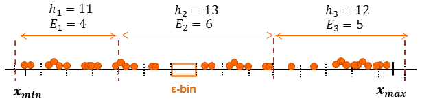
Figure 1: A possible choice of intervals, with their respective data-counts $(h_{k})_{1\leq k\leq K}$ and lengths expressed in number of $\epsilon$-bins $(E_{k})_{1\leq k\leq K}$.

They are the building blocks of histogram intervals: possible grouping of consecutive $\epsilon$-bins into $K$ intervals, with $K$ ranging from 1 to $E$, defines a histogram. A histogram $\mathcal{M}$ is fully specified by $\mathcal{M}=(K,C,(h_{k})_{1\leq k\leq K})$ where $K$ is the number of intervals, $C=(c_{k})_{0\leq k\leq K}\subset\mathcal{C}$ are the endpoints and $h_{k}$ are the counts in each bin (we have $c_{0}=x_{\min}-\epsilon/2$ and $c_{K}=x_{\max}+\epsilon/2$). Notice that such a histogram is not bound to any given data set, despite the use of the term “counts” for the $h_{k}$. Most of the methods studied in this paper, including our proposals, follow a maximum likelihood principle and therefore given $K$ and $\mathcal{C}$, the $h_{k}$ will be directly computed from the observations. Considering arbitrary histograms is nevertheless useful to include non maximum likelihood methods such as the taut string approach from Davies and Kovac (2004); Davies et al. (2009), and to define easily prior distributions on histograms (see Section 5.1.1).

The piecewise constant density associated to $\mathcal{M}=(K,C,(h_{k})_{1\leq k\leq K})$ is given by

$$f_{\mathcal{M}}(x)= \frac{1}{n}\sum_{k=1}^{K}\frac{h_{k}}{c_{k}-c_{k-1}}\mathbb{I}_{]c_{k-1},c_{k}]}(x),$$ (2)

$$= \frac{1}{n\epsilon}\sum_{k=1}^{K}\frac{h_{k}}{E_{k}}\mathbb{I}_{]c_{k-1},c_{k}]}(x),$$

where $E_{k}$ is the number of $\epsilon$-bins in interval $[c_{k-1},c_{k}]$, $n=\sum_{k=1}^{K}h_{k}$ and $\mathbb{I}_{A}$ is the indicator function of the set $A$. Notice that the intervals are exclusive of their lower bound, even for the first interval $]c_{0},c_{1}]$. This is by virtue of the definition of $c_{0}$ which is outside of the range of the data: no observation can be missed despite the exclusion of $c_{0}$ from the formal definition of the density. This enables us to keep a simple notation but it has no effect on the rest of the analysis.

3.2 Dynamic programming

While the two classical restrictions over the partitions we highlighted (data-driven grids and fixed grids) make the optimisation space finite, it remains large. There are $E\choose K-1$ different partitions of $E$ elementary bins in $K$ intervals, and $E$ may be big. However, most criteria used in the literature are additive and can therefore be optimised using the dynamic programming principle (Bellman, 1961). This was proposed originally in Kanazawa (1988) for irregular histograms with endpoints constrained to observations. Since then, dynamic programming has been used systematically for all irregular histogram estimation techniques we are aware of.

Provided the chosen criterion can be computed efficiently, dynamic programming has a computational complexity of $\mathcal{O}(E^{2}\cdot K_{max})$ when the histograms have at most $K_{max}$ bins (and thus a maximal complexity of $\mathcal{O}(E^{3})$).

3.3 Data driven grid versus fixed grid

Both finite grids have advantages and drawbacks. Data driven grids do not introduce an additional precision parameter but this comes with a potential large computational cost. Dynamic programming has a computational cost of $\mathcal{O}(n^{2}\cdot K_{max})$ for a data driven grid with $n$ observations and a limit of $K_{max}$ bins in the histograms. If one sets $K_{max}=n$ to avoid introducing yet another parameter, data driven grids lead to a cubic cost $\mathcal{O}(n^{3})$ and thus do not scale to large data sets. To circumvent this problem (Rozenholc et al., 2010) use a greedy clustering of the data driven grid into $\max(n^{\frac{1}{3}},100)$ bins prior to applying a dynamic programming approach. This blurs the distinction between data driven grids and fixed ones, and introduces a new parameter (the cut-off value of 100 used in Rozenholc et al. (2010)).

Another limitation of data driven grids is that they assume a perfect representation of real numbers. This is acceptable for small data sets but for large scale data sets, the probability of getting identical observations increases and the limits of real number representation start to play a role. This problem is discussed in Knuth (2019); Knuth et al. (2006) and in Section 6.2.

Finally in a Bayesian perspective, endpoints prior distributions have to be specified. With a data driven grid, continuous densities are needed while discrete distributions are needed when using a fixed grid. As a consequence, specifying priors that favor simple histograms is easier in the discrete case than in the continuous one.

Fixed grids bypass the above issues, at the cost of introducing a new accuracy parameter. We propose in Section 5.2 a way to automate the choice of this parameter. This mitigates the drawbacks of the fixed grid, while keeping all its advantages.

4 An NML criterion for histogram density estimation

Among minimum description length approaches, Kontkanen and Myllymäki’s solution (Kontkanen and Myllymäki, 2007) derived using the Normalized Maximum Likelihood (NML) is the closest to our proposal. This approach consists in minimising a criterion $c_{\leavevmode\nobreak\ \textnormal{NML}}$ over all possible histograms defined on a fixed grid as in Section 3.1. The criterion is evaluated for a data set $D=(x_{i})_{1\leq i\leq n}$ of $n$ observations.

To ease the comparison of this criterion to our own, we report the following simplified expression for $c_{\leavevmode\nobreak\ \textnormal{NML}}$, using notations of Section 3.1 (the derivation is provided in A):

$$c_{\leavevmode\nobreak\ \textnormal{NML}}(\mathcal{M}|D)= \log\binom{E}{K-1}+\log\leavevmode\nobreak\ {\mathcal{R}}^{n}_{\mathcal{M}}$$ (3)

$$+\log\frac{n^{n}}{{h_{1}}^{h_{1}}\dotsm{h_{K}}^{h_{K}}}+\sum^{K}_{k=1}h_{k}\log E_{k},$$

where $\log\leavevmode\nobreak\ {\mathcal{R}}^{n}_{\mathcal{M}}$ is called the NML parametric complexity. Notice that the $h_{k}$ are computed from the data set $D$ based on the histogram specification (see Section 5.1.2 for a discussion on this aspect).

The NML parametric complexity can be interpreted as the logarithm of the number of different distributions for a given model class (Grunwald, 2007). The term $\log\binom{E}{K-1}$ represents the code length of the choice of $K-1$ cut-points among the $E$ possible candidates. Notice that this term is not directly derived from the NML distribution but was added by the authors as a way to index the different model choices, as recommended in Grunwald (2007). The last two terms represent the log-likelihood of the partition of $n$ entries into $K$ parts of size $(h_{k})_{1\leq k\leq K}$ and the log-likelihood of data distribution within each interval respectively.

The NML density has several important theoretical optimality properties: it is the minimax optimal universal model (Shtarkov, 1987). Additionally, codes that are derived from it minimize the expected regret when choosing the worst-case generating density model for the data (Rissanen, 2001). In Kontkanen and Myllymäki (2007), the authors show how to find the NML-optimal cut points via a dynamic programming in a polynomial time with respect to $E$, the total number of cut-points available for selection. Furthermore, their experiments showed that the minimization of the NML criterion produced good quality histograms of several Normal distributions of $n=10,000$ samples, all for a fixed approximation accuracy ($\epsilon=0.1$).

We argue however that the NML approach has the following limitations.

NML computation:

the NML approach results in a criterion whose exact computation remains costly. The cost of computing the NML parametric complexity was reduced from $\mathcal{O}(n^{2})$ (Kontkanen et al., 2003) to $\mathcal{O}(n+K)$ algorithm in Kontkanen and Myllymäki (2007).

Approximations of the NML parametric complexity have been introduced to reduce its computation time. For instance a $\mathcal{O}(\sqrt{dn}+K)$ algorithm (where $d$ is the precision in digits) is given in Mononen and Myllymäki (2008). Szpankowski proposes in Szpankowski (1998) an approximate computation in $O(1)$ time but with an asymptotical error in $\mathcal{O}(n^{-3/2})$. The trade-off of using these faster methods is either a loss in precision or an error that is hard to evaluate non asymptotically w.r.t. n and K.

Notice that the main issue of the computational cost of the NML complexity is induced by the need to evaluate it at least $\mathcal{O}(n)$ times to build an optimal histogram, leading to minimal total cost of $\mathcal{O}(n^{2})$ for an exact calculation.

Choice of $\epsilon$:

Although the authors argue that the sole user-defined parameter $\epsilon$ does not play a role in the model selection process, we show on the contrary in Section 6.2 that its impact cannot be overlooked. An automated choice is therefore needed.

Notice also that (Kontkanen and Myllymäki, 2007) uses a dynamic programming approach to optimise $c_{\leavevmode\nobreak\ \textnormal{NML}}$ which has a $\mathcal{O}(E^{2}\cdot K_{max})$ or a $\mathcal{O}(E^{3})$ computational cost, as already explained in Section 3.2.

We improve over the NML approach on those three issues by introducing in Section 5 an enumerative criterion that avoids the NML computation cost, in Section 5.2 a granulated version of the our criterion that automates the choice of the precision parameter and finally in Section 7 greedy search heuristics that together reduce the global computational cost from $\mathcal{O}(E^{3})$ to $\mathcal{O}(n\log n)$.

5 G-Enum: a granulated enumerative criterion

This paper’s first contribution is the introduction of a granulated enumerative two-part code for histogram density estimation, which we call G-Enum. It builds on a simpler enumerative approach, for which we introduce granularity later.

5.1 Enumerative criterion

Our enumerative criterion for histogram model selection exploits a maximum a posteriori Bayesian interpretation of the MDL principle which has the same optimality properties as the NML distribution (Boullé et al., 2016). In this framework, the best model is the one that maximises the probability of the model given the data, $p(\mathcal{M}|D)$ where $D=(x_{i})_{1\leq i\leq n}$ is a data set of $n$ observations (we allow non unique values in $D$). This formulation is well known to be equivalent to a penalised likelihood approach. Indeed we have

$$\log p(\mathcal{M}|D)=\log p(\mathcal{M})+\log p(D|\mathcal{M})-\log p(D).$$

As $\log p(D)$ does not depend on $\mathcal{M}$, maximising $p(\mathcal{M}|D)$ is equivalent to maximising a compromise between a large likelihood $\log p(D|\mathcal{M})$ and a small prior probability $\log p(\mathcal{M})$ for a complex model and the reverse for a simple one. In practice, we minimise an enumerative criterion

$$c_{\leavevmode\nobreak\ \textnormal{Enum}}(\mathcal{M}|D)=-\log p(\mathcal{M})-\log p(D|\mathcal{M}).$$ (4)

5.1.1 Prior distribution

Using notations from Section 3.1, where $K$ is the number of intervals, $C$ is the set of endpoints of the histograms invertals and $\{h_{k}\}$ are the counts of values in each of these intervals, we factor $p(\mathcal{M})$ as

$$p(\mathcal{M})=p(K)\cdot\leavevmode\nobreak\ p(C|K)\cdot\leavevmode\nobreak\ p ((h_{k})_{1\leq k\leq K}|K,C),$$

without loss of generality. Then, we use a hierarchical prior on the parameters and we assume conditional independence of $C$ and $\{h_{k}\}_{1\leq k\leq K}$ given $K$. Thus, we have

$$p(\mathcal{M})=p(K)\cdot\leavevmode\nobreak\ p(C|K)\cdot\leavevmode\nobreak\ p ((h_{k})_{1\leq k\leq K}|K),$$

with the following components:

• Number of intervals

  For the number of intervals $K$, we could use a uniform prior distribution leading to $p(K)=\frac{1}{E}$, but Rissanen’s universal prior for integers (Rissanen, 1983) is more adapted as it favors small integers, i.e. simpler histograms. We have

  $$p(K)=\exp(-\log^{*}K),$$ (5)

  with $\log^{*}K=\log_{2}\left(\kappa_{0}\right)+\sum_{j>1}\max\left(\log_{2}^{(j)}(K),0\right)$, where $\kappa_{0}=\sum_{p>1}2^{-\log_{2}^{*}(p)}=2.865$ and $\log_{2}^{(j)}(K)$ is the $j$-th composition of $\log_{2}$, i.e. $\log_{2}^{(1)}(K)=\log_{2}(K)$ and $\log_{2}^{(j)}(K)=\log_{2}(\log_{2}^{(j-1)}(K))$.

  For the rest of the parameters, we use uniform priors.

• Interval composition

  Specifying interval endpoints $C$ is equivalent to specifying the number of elementary bins gathered into each interval. We use a uniform distribution over all the ordered partitions of the $E$ elementary bins into $K$ contiguous subsets of size $E_{1},E_{2},\dots E_{K}$ such that $E_{1}+E_{2}+\dots+E_{K}=E$. We allow empty subsets, which leads to

  $$p(C|K)=\frac{1}{\binom{E+K-1}{K-1}}.$$ (6)

  Notice that we could forbid empty subsets (i.e. identical endpoints) which would lead to $p(C)=\frac{1}{\binom{E}{K-1}}$ but this later solution is non monotone with respect to $K$ and favors values around $\frac{E}{2}$ which is not a desirable property.

• Prior on $(h_{k})_{1\leq k\leq K}$

  For a given number of intervals $K$, the $(h_{k})_{1\leq k\leq K}$ specify the number of observations in each interval. A value for $\{h_{k}\}_{1\leq k\leq K}$ is therefore a vector of $K$ non negative integers which sum to $n$. There are of $\binom{n+K-1}{K-1}$ such vectors and we use a uniform distribution over them, leading to

  $$p((h_{k})_{1\leq k\leq K}|K)=\frac{1}{\binom{n+K-1}{K-1}}$$ (7)

5.1.2 Likelihood

The likelihood $p(D|\mathcal{M})$ is obtained using a generative model for histograms specified by $\mathcal{M}$ which is also based on uniform distributions. Importantly, we do not assume the observations to be independent, contrarily to most of the histogram models.

Notice also that the $\{h_{k}\}_{1\leq k\leq K}$ in $\mathcal{M}$ are not computed from the data but parameters. This means that $p(D|\mathcal{M})$ is non zero if and only if $\mathcal{M}$ and $D$ are compatible.

Definition 1.

A data set $D=(x_{i})_{1\leq i\leq n}$ and a histogram $\mathcal{M}=(K,C,(h_{k})_{1\leq k\leq K})$ are compatible if and only if

$$\forall k\in\{1,\ldots,K\},\left|\left\{i\in\{1,\ldots,n\}\mid x_{i}\in]c_{k-1},c_{k}]\right\}\right|=h_{k},$$

where $|S|$ denotes the cardinal of set $S$.

Notice that in practice the data “set” $D$ can contain multiple times the same value and thus we take into account the index set when counting observations in this definition (see Section 6.2 for additional details on this aspect).

Given $\mathcal{M}$, a data set $D$ is generated by a hierarchical distribution based on uniform distributions.

1. Observations are generated by first choosing which interval is responsible for generating each individual observation. This corresponds to building a mapping $I_{map}$ from $1,\ldots,n$ to $1,\ldots,K$ specifying that $x_{i}$ will be generated in interval $I_{map}(i)$. $I_{map}$ is compatible with $\mathcal{M}$ if

   $$\forall k\in\{1,\ldots,K\},\left|\left\{i\in\{1,\ldots,n\}\mid I_{map}(i)=k\right\}\right|=h_{k}.$$

   There are $\frac{n!}{h_{1}!...h_{K}!}$ such mappings and we assume a uniform distribution on them, that is

   $$p(I_{map}|\mathcal{M})=\frac{h_{1}!...h_{K}!}{n!}$$ (8)

2. Then given $I_{map}$ we generate observations assigned independently to distinct intervals, i.e.

   $$p(D|I_{map},\mathcal{M})=\prod_{k=1}^{K}p((x_{i})_{I_{map}(i)=k}|\mathcal{M}).$$ (9)

3. In a given interval, observations are generated by choosing their elementary bins independently and uniformly. That is we assume

   $$p((x_{i})_{I_{map}(i)=k}|\mathcal{M})=\left(\frac{1}{E_{k}}\right)^{h_{k}},$$ (10)

   as there are $E_{k}$ elementary bins in interval $k$ and we have $h_{k}$ data points to generate. Notice than if $h_{k}=0$, then we can have $E_{k}=0$ as in this case $\forall i,\ I_{map(i)}\neq k$ by compatibility.

Then when $\mathcal{M}$ and $D$ are compatible, we have

$$p(D|\mathcal{M})=\frac{h_{1}!...h_{K}!}{n!}\cdot\prod^{K}_{k=1}\left(\frac{1}{E_{k}}\right)^{h_{k}}.$$ (11)

The simple enumerative criterion for histogram density estimation is thus given by

$$c_{\leavevmode\nobreak\ \textnormal{Enum}}(\mathcal{M}|D)= \log^{*}K+\log\binom{E+K-1}{K-1}$$

$$+\log\binom{n+K-1}{K-1}$$

$$+\log\frac{n!}{h_{1}!...h_{K}!}+\sum^{K}_{k=1}h_{k}\log E_{k}.$$ (12)

We use the convention that $0\times\log 0=0$ to avoid the case where $h_{k}=0$. Notice that equation (5.1.2) is valid only when $\mathcal{M}$ and $D$ are compatible. When $\mathcal{M}$ and $D$ are not compatible, $p(D|\mathcal{M})=0$ and we set accordingly $c_{\leavevmode\nobreak\ \textnormal{Enum}}(\mathcal{M}|D)=+\infty$. As a consequence, histograms that are not compatible with the data are excluded from the solution space of our approach. This ensure that histograms obtained by minimizing the proposed criterion use a classical maximum likelihood estimation of the density in each of their intervals.

5.1.3 Comparison to the NML criterion

A side by side comparison of the Enum and NML criteria terms is presented in table 1.

Table 1: Term comparison of the NML and enumerative criteria

Crit.	Indexing terms	Multinomial terms	Bin index terms
NML Kontkanen and Myllymäki (2007)	$\displaystyle\log\binom{E}{K-1}$	$\displaystyle\log\leavevmode\nobreak\ {\mathcal{R}}^{n}_{\mathcal{M}}+\log\frac{n^{n}}{{h_{1}}^{h_{1}}\dotsm{h_{K}}^{h_{K}}}$	$\displaystyle\sum^{K}_{k=1}h_{k}\log E_{k}$
Enum	$\displaystyle\log^{*}K+\log\binom{E+K-1}{K-1}$	$\displaystyle\log\binom{n+K-1}{K-1}+\log\frac{n!}{h_{1}!...h_{K}!}$	$\displaystyle\sum^{K}_{k=1}h_{k}\log E_{k}$

The terms that represent the indexing of $\epsilon$-bins within each interval are exactly the same for both criteria. The differences lie in model indexing and the encoding of the multinomial distributions.

Model indexing terms

As in the NML criterion, we too have a term that serves as an index for model families. In the Enum criterion, model indexing is done through a $\log\binom{E+K-1}{K-1}$ term. This term is monotone with $K$: it penalizes models with many intervals. The corresponding term in the NML criterion is not monotone and might thus favour choices with many cut-points (especially when $K\sim E$).

Multinomial terms

These terms encode the multinomial distributions of $n$ observations into $K$ intervals. Both versions are universal codes (Grunwald, 2007) and have been proved to have the same optimality properties (Boullé et al., 2016). What sets them apart is that the enumerative version is easier to compute and to analyze.

The classical NML parametric complexity ($\log\leavevmode\nobreak\ {\mathcal{R}}^{n}_{\mathcal{M}}$) is replaced by a simpler term in the Enum approach ($\log\binom{n+K-1}{K-1}$). As shown in Kontkanen and Myllymäki (2007), the NML complexity can be computed exactly in $\mathcal{O}(n+K)$ time. In stark contrast, the equivalent term in our enumerative criterion can be computed in $\mathcal{O}(1)$ time.

As we can see, both criteria are very similar, though the Enum criterion is clearly simpler to compute and to analyse theoretically, using its closed form expression (see Section 6).

5.2 G-Enum criterion

The Enum criterion solves the computational issues induced by the NML parametric complexity without introducing approximations, but we still have to choose the approximation accuracy $\epsilon$ associated to the fixed grid. We introduce granularity to mitigate this issue.

Granularity and $\epsilon$

The main issue with $\epsilon$ is that it plays two roles. It serves as a way to set a precision limit for the representation of real numbers, as discussed in Section 3.3. It also plays a crucial role in setting the resolution of the histograms themselves through $E$. The first role is more related to the data collection process and to the way the fixed grid is specified than to modelling, while the second appears directly in the model selection process via $E$.

We propose to explicitly separate those roles by introducing an intermediate parameter $G$, the granularity. For a given $E$, we assume that the numerical domain can be split into $G$ bins ($1\leq G\leq E$) of equal width. Each of these new elementary bins, that we call $g$-bins, is composed of $g=E/G$ $\epsilon$-bins. Each of the intervals of any constructed histogram has a length that is a multiple of these $g$-bins. In other words, each interval is no longer composed of a multiple of $\epsilon$-bins but rather composed of $G_{k}$ $g$-bins. To better grasp this new setting, Figure 2 shows the case where three intervals were made from $g$-bins. In this illustration, we have $E=20$ and $G=5$, so that each $g$-bin is composed of $4$ $\epsilon$-bins.

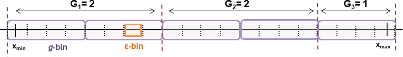
Figure 2: Replacing $\epsilon$-bins by $g$-bins in the model building

By keeping $\epsilon$, we still have a fixed grid and user defined resolution for both the data and the grid itself, while the introduction of $G$ enables to chose the overall maximal complexity of the histogram.

Granulated criterion

Each granulated bin can either contain a whole number or a fraction of $\epsilon$-bins. To simplify our reasoning and keep this paper self-contained, we assume that the number of elementary $\epsilon$-bins E is a multiple of G, i.e. $g=E/G\in\mathbb{N}^{*}$.

Using this new parameter, the criterion changes both in model indexing terms and in the bin indexing terms:

• change in model indexing terms  If we assume that $G$ is distributed according to the universal prior for integers, the prior term for choosing the length of the intervals turns from $\displaystyle\log\binom{E+K-1}{K-1}$ into $\displaystyle\log^{*}G+\log{{G+K-1}\choose{K-1}}$.

• change in bin indexing terms  Interval lengths are no longer described by $E_{k}$ $\epsilon$-bins but rather by $G_{k}$ $g$-bins. Given that each $g$-bin is actually an aggregation of $g=E/G$ $\epsilon$-bins, the likelihood term of the data distribution within an interval is now given by:

  $$\sum^{K}_{k=1}h_{k}\log\left(G_{k}\cdot\frac{E}{G}\right) =\sum^{K}_{k=1}h_{k}\log G_{k}+\sum^{K}_{k=1}h_{k}\log\frac{E}{G}$$

  $$=\sum^{K}_{k=1}h_{k}\log G_{k}+n\log\frac{E}{G}$$ (13)

This new criterion, which we call G-Enum is very similar to the original criterion introduced in this paper, as shown in table 2. The accuracy $\epsilon$ remains under the control of the user and can be fixed using standard considerations on real number computer representation (see Section 6.2), all the while $G$ is optimised as part of model selection.

Table 2: Term comparison of the Enum and G-Enum criteria

Crit.	Indexing terms	Multinomial terms	Bin indexing terms
Enum	$\displaystyle\log^{*}K+\log\binom{E+K-1}{K-1}$	$\displaystyle\log\binom{n+K-1}{K-1}+\log\frac{n!}{h_{1}!...h_{K}!}$	$\sum^{K}_{k=1}h_{k}\log E_{k}$
G-Enum	$\displaystyle\log^{*}K+\log^{*}G+\log{{G+K-1}\choose{K-1}}$	$\displaystyle\log\binom{n+K-1}{K-1}+\log\frac{n!}{h_{1}!...h_{K}!}$	$\sum^{K}_{k=1}h_{k}\log G_{k}+n\log\frac{E}{G}$

6 Theoretical properties

An analytical study of both the Enum and G-Enum criteria provides insights into how the enumerative MDL criterion works. Most of the propositions that follow cannot be extended to the NML criterion because of the non-monotone nature of some of its terms and because of the lack of closed-form expression for the parametric complexity. We focus solely on Enum and G-Enum histograms in what follows, as only these criteria are fit for analysis.

6.1 Compelling properties of enumerative histograms

We study the behaviour of the criterion in certain configurations in order to identify the most important factors that determine the overall shape of an optimal histogram (proofs of these properties are provided in B). Notice that although our analysis focuses on the encoding vision of the criterion, these properties can also be understood as statements of the most likely outcomes in terms of probability. This is due to the natural link between a coding length (the criterion value) and a posteriori probability at the basis of information theory: a more probable model will have a shorter coding length. Note also that in the properties, models are always assumed to be compatible with the data.

We show first an elementary property of optimal histograms.

Proposition 1.

Let $\mathcal{M}=(K,(c_{k})_{0\leq k\leq K},(h_{k})_{1\leq k\leq K})$ be an optimal histogram for the data set $D$. Then

$$\forall k,1\leq k\leq K\ c_{k-1}<c_{k}.$$

In other words, an optimal histogram cannot contain zero-length intervals.

Then we show that too complex histograms will not be selected by our criterion.

Proposition 2.

Let $D$ be a data set with $n$ observations. Let us denote $\mathcal{M}_{K=n}$ a histogram compatible with $D$ such that there is one observation per interval and $\mathcal{M}_{K=1}$ a histogram compatible with $D$ with only one interval. Then the coding length of $\mathcal{M}_{K=1}$ is shorter than the one of $\mathcal{M}_{K=n}$:

$$c_{\leavevmode\nobreak\ \textnormal{Enum}}(\mathcal{M}_{K=n}|D)>c_{\leavevmode\nobreak\ \textnormal{Enum}}(\mathcal{M}_{K=1}|D).$$

This can be extended to more complex solutions with empty intervals.

Proposition 3.

Let $D$ be a data set with $n$ observations. Let us denote $\mathcal{M}_{K>n}$ a histogram compatible with $D$ consisting of either singleton or empty intervals, one interval for each observation and empty intervals in-between, and let $\mathcal{M}_{K=1}$ be as in Proposition 2. Then the coding length of $\mathcal{M}_{K=1}$ is shorter than the one of $\mathcal{M}_{K>n}$:

$$c_{\leavevmode\nobreak\ \textnormal{Enum}}(\mathcal{M}_{K>n}|D)>c_{\leavevmode\nobreak\ \textnormal{Enum}}(\mathcal{M}_{K=1}|D).$$

In addition, optimal histograms will never exhibit two consecutive empty intervals.

Proposition 4.

For any data set $D$, the coding length of a histogram with two adjacent empty intervals is always longer than the coding length of a histogram with no consecutive empty intervals.

$$c_{\leavevmode\nobreak\ \textnormal{Enum}}(\mathcal{M}_{K,(h_{A},h_{B})=0}|D)>c_{\leavevmode\nobreak\ \textnormal{Enum}}(\mathcal{M}_{K-1,h_{A\cup B}=0}|D)$$

Despite those general rules, local optimisation remains possible in the sense that empty intervals or intervals with only a single observation can be present in optimal histograms.

Proposition 5.

There exist data sets such that the optimal histogram has at least one interval which contains only a single observation.

Proposition 6.

There exist data sets such that the optimal histogram has at least one interval that does not contain any observation.

We can also characterise the structure of optimal histograms in different ways.

Proposition 7.

An optimal histogram has at most $2n-2$ intervals ($K^{*}\leq 2n-2$).

Proposition 8.

In an optimal histogram, each interval endpoint is at most $\epsilon$ away from one of the values of the data set.

Propositions 4, 7 and 8 will serve as the basis for further improvements on the search of the best histogram. For instance, as Proposition 4 states that an optimal histogram will not have consecutive empty intervals, our search heuristic will systematically favour the merge of two consecutive empty bins. See Section 7 for additional details.

6.2 Role of the approximation accuracy $\epsilon$

The authors of the NML criterion argue that the effect of the approximation accuracy $\epsilon$ can be ignored during the model selection process (Kontkanen and Myllymäki, 2007) and set to the accuracy at which the data have been recorded. In their experiments, $\epsilon$ is fixed to a rather large value ($0.1$) which is inconsistent with current recording practices.

In this section, we conduct a theoretical investigation of the behaviour of the Enum criterion when $\epsilon\rightarrow 0$ (or equivalently, when $E\rightarrow\infty$). Experimental results illustrate this behaviour in Section F.

6.2.1 Behaviour when $\epsilon\rightarrow 0$

To study the behaviour of our enumerative criterion as $\epsilon$ tends to 0, we first introduce the definition of singular intervals.

Definition 2.

Let $\mathcal{M}=(K,C,(h_{k})_{1\leq k\leq K})$ be a histogram compatible with a data set $D$ and built on a $\epsilon$ grid. An interval $I_{k}=]c_{k-1},c_{k}]$ of $\mathcal{M}$ is singular if the following conditions are met

1. $c_{k}-c_{k-1}=\epsilon$;

2. $h_{k}>0$;

3. all values of $D$ that belong to $I_{k}$ are identical.

We denote by $S(\mathcal{M},D)$ the number of data points from $D$ that belong to singular intervals. In other words

$$S(\mathcal{M},D)=\sum_{I_{k}\text{ is singular}}h_{k}.$$

Then we have the following theorem (see C for the proof).

Theorem 1.

Let $D$ be a data set with $n$ observations. There exists two positive values $C(D)$ and $E(D)$ that depends only on $D$ such that for all $\epsilon\leq E(D)$ for any optimal histogram $\mathcal{M}^{\star}$ have

$$\begin{split}\left|c_{\leavevmode\nobreak\ \textnormal{Enum}}(\mathcal{M}^{\star}|D)-\left\{K-1+n-S(\mathcal{M}^{\star},D)\right\}\log\frac{1}{\epsilon}\right|\\ \leq C(D).\end{split}$$ (14)

As $c_{\leavevmode\nobreak\ \textnormal{Enum}}(\mathcal{M}^{\star}|D)$ is dominated by the $\log\frac{1}{\epsilon}$ term when $\epsilon\rightarrow 0$, equation (14) shows that there is an inherent trade off between $K$ and $S(\mathcal{M}^{\star},D)$. With a higher value of $K$, a histogram has more opportunities to have singular intervals and thus to have a larger value of $S(\mathcal{M}^{\star},D)$. If $D$ contains multiple instances of the same value (i.e. there are $i$ and $j$ such that $i\neq j$ and $x_{i}=x_{j}$), $S(\mathcal{M}^{\star},D)$ can grow fast enough to compensate the increase of $K$ and it is therefore not possible to characterise further the asymptotic behaviour of $c_{\leavevmode\nobreak\ \textnormal{Enum}}(\mathcal{M}^{\star}|D)$.

However in the particular case where all values are distinct in $D$, we have the following corollary (see C for the proof).

Corollary 1.

Let $D$ be a data set with $n$ distinct observations. Then for $\epsilon$ sufficiently small, the optimal histogram build on $\epsilon$ bins for the Enum criterion is the trivial one with a single interval

$$\mathcal{M}=(1,\{x_{\min}-\frac{\epsilon}{2},x_{\max}+\frac{\epsilon}{2}\},n).$$

Enumerative histograms have a detrimental asymptotic behaviour: if we strive to be more precise in terms of cut point positions, the quality of the model will be poorer.

6.2.2 Illustration of the asymptotic behaviour

To complement the asymptotic analysis provided by Theorem 1 and its corollary, we study a simple example in the present section. Experiments on synthetic data are provided in F.

Let $\mathcal{U}[a,b]$ denote the uniform distribution on the interval $[a,b]$. Let $\alpha$ and $\theta$ be two real numbers with $\alpha\in]0,\frac{1}{2}]$ and $\theta\in]\frac{1}{2},1]$. Let us consider a data set $D_{n}(\theta,\alpha)$ consisting of $n\theta$ independent observations generated by $\mathcal{U}[0,\alpha]$ and $n(1-\theta)$ independent observations generated by $\mathcal{U}[\alpha,1]$.

An optimal histogram should contain two intervals with a cut point close to $\alpha$, provided that the mixture density $\theta\mathcal{U}[0,\alpha]+(1-\theta)\mathcal{U}[\alpha,1]$, is distinct enough from $\mathcal{U}[0,1]$. However Corollary 1 applies and if the precision $\epsilon$ is small enough, a single interval will be preferred. We can study on this simple example the relationship between $\epsilon$, $n$ and the mixture density to get a better understanding of the limitations proved by our results.

We study the optimal histogram with a unique interval, $\mathcal{M}^{\star}_{1,\epsilon}$ as well as the ideal histogram with two intervals $\mathcal{M}^{\star}_{2,\epsilon}$ with a cut point in $\alpha$. Let $\Delta(n,\epsilon,\alpha,\theta)$ be

$$\Delta(n,\epsilon,\alpha,\theta)=c_{\leavevmode\nobreak\ \textnormal{Enum}}(\mathcal{M}^{\star}_{2,\epsilon}|D_{n}(\theta,\alpha))-c_{\leavevmode\nobreak\ \textnormal{Enum}}(\mathcal{M}^{\star}_{1,\epsilon}|D_{n}(\theta,\alpha)).$$

We show in D that

$$\Delta(n,\epsilon,\alpha,\theta)= \log\left(\frac{1}{\epsilon}+1\right)-nD_{KL}(\theta\|\alpha)+O(\log n),$$

where $D_{KL}(\theta\|\alpha)$ is Kullback-Leibler divergence between the Bernoulli distribution with parameter $\theta$ ($\mathcal{B}(\theta)$) and the one with parameter $\alpha$ ($\mathcal{B}(\alpha)$). The histogram with two intervals is the optimal one if $\Delta(n,\epsilon,\alpha,\theta)<0$.

For a fixed value of $\epsilon$, the histogram with two intervals is preferred for larger values of $n$. The value of $n$ needed to induce this preference is reduced by an increased $KL$ divergence between $\mathcal{B}(\theta)$ and $\mathcal{B}(\alpha)$. An important aspect is that $E=\frac{1}{\epsilon}$ influences the criterion in a logarithmic way while the influence of $n$ is linear. This means that, in this example, large values of $E$ can be compensated by relatively small values of $n$.

To illustrate further the behaviour, we computed exactly $\Delta(n,\epsilon,\alpha,\theta)$ for $\theta=1/2$ and $\alpha=1/10$, and for different values of $n$ and $E$. Table 3 summarizes those results by showing for several $n$ the minimum value of $E$ above which the single interval solution is preferred over the two interval ones.

Table 3: Transition from two intervals to one single interval.

$n$	$E$
10	$30$
12	$80$
16	$530$
20	$3700$
30	$5.05\times 10^{5}$
40	$7.28\times 10^{7}$
50	$1.08\times 10^{10}$

In this simple and extreme example, the transition appears only for very large values of $E$. However, as shown in F, in more realistic settings the effects of $E$ manifests in a more reasonable range of values justifying the need for selecting it (or equivalently $\epsilon$) carefully.

6.3 Behaviour of the G-Enum criterion

While the decoupling between the precision of the grid and the resolution of the histograms provided by the G-Enum enables us to optimise the latter, it does not change the properties of the criterion for a fixed value of $G$.

This can be seen by interpreting a histogram $\mathcal{M}$ computed on $G$ g-bins constructed from $\epsilon$-bins as if it was constructed directly on g-bins. In other words, we can compute its quality according to the G-Enum criterion, taking into account the underlying $\epsilon$-bins or according to the Enum criterion in which $E$ is set to $G$. Then we have

$$c_{\leavevmode\nobreak\ \textnormal{G-Enum}}(\mathcal{M},D)_{G,E}=c_{\leavevmode\nobreak\ \textnormal{Enum}}(\mathcal{M},D)_{G}+\log^{*}G+n\log{\frac{E}{G}},$$

where the dependency to $G$ and $E$ has been made explicit using subscripts.

This means that all propositions established for the Enum criterion still hold for the G-Enum criterion, for any fixed $G$ parameter. In addition, the best histogram for G-Enum when $G$ is fixed to a given value is exactly the best histogram for Enum with $E=G$. Thus, we can use any optimisation strategy designed to find the best Enum histogram to obtain the best G-Enum histogram for any fixed value of $G$.

Moreover, if we consider two different values of $G$, $G_{1}$ and $G_{2}$, both divisors of $E$, we have

$$c_{\leavevmode\nobreak\ \textnormal{G-Enum}}(\mathcal{M},D)_{G_{1},E}-c_{\leavevmode\nobreak\ \textnormal{G-Enum}}(\mathcal{M},D)_{G_{2},E}=c_{\leavevmode\nobreak\ \textnormal{Enum}}(\mathcal{M},D)_{G_{1}}-c_{\leavevmode\nobreak\ \textnormal{Enum}}(\mathcal{M},D)_{G_{2}}+\log^{*}G_{1}-\log^{*}G_{2}+n\log\frac{G_{2}}{G_{1}}.$$

This shows that the optimal model for G-Enum depends only in a limited way on $E$. The choice of $E$ simply constrains the possible values of $G$ to its divisors, which in turn constrains the space of possible histograms. Importantly, in this space, the choice of the optimal histogram does not depend on $E$.

Notice also that while the G-Enum criterion does no longer suffer from the increase of $E$, it will behave similarly as $G$ increases: for distinct data points, when $G$ is larger than a data dependent bound $G_{\max}(D)$ the optimal histogram for a fixed $G$ consists in a single interval.

As a counter measure, we propose to set $E$ to a very large value using the limits of numerical representation precision as a guideline. Given that integer values are encoded using four bytes and have their values between $\textnormal{INT}_{\min}\approx-2.10^{9}$ and $\textnormal{INT}_{\max}\approx 2.10^{9}$, one can set $E$ up to $E_{\max}=10^{9}\approx\textnormal{INT}_{\max}/2$.

Then we can select a set of values of $G$ among the divisors of $E$, compute the optimal histogram for each of those values according to Enum and select the best overall one using G-Enum. Details about this procedure are given in Section 7.3.

7 Efficient search for MDL-optimal histograms

As recalled in Section 3.2, most irregular histogram construction methods leverage the dynamic programming principle to obtain an optimal histogram (with respect to the chosen criterion). This is in particular the case of the NML approach which has as a consequence a $\mathcal{O}(E^{3})$ complexity (Kontkanen and Myllymäki, 2007).

We describe in this Section several techniques used to reduce this complexity. First, we introduce a greedy approach that can be applied to any additive criterion to obtain in $\mathcal{O}(E\log E)$ time a sub-optimal histogram of good quality. Then, we show how to reduce this complexity to $\mathcal{O}(n\log n)$ leveraging properties of enumerative histograms. Finally, we detail and discuss the particularities of the optimisation of granular models.

7.1 Greedy search

We propose a greedy search heuristic that combines a classic bottom-up approach and post-optimisations. It is based on a similar greedy algorithm to minimize additive criteria in the case of supervised discretisation (Boullé, 2006). It applies to any additive criterion, defined as follows.

Definition 3.

Let $\mathcal{M}=(K,C,(h_{k})_{1\leq k\leq K})$ be a histogram compatible with a data set $D$ of size $n$. The histogram is based on the intervals $]c_{k-1},c_{k}]$ defined by $C=(c_{k})_{0\leq k\leq K}$. A criterion that evaluate the quality of $\mathcal{M}$ with respect to $D$, $q(\mathcal{M}|D)$, is additive if it can be written

$$q(\mathcal{M}|D)=q_{1}(n,K)+\sum_{k=1}^{K}q_{2}(c_{k-1},c_{k},h_{k}).$$

The main consequence of using an additive criterion is it locality. For instance when two adjacent intervals are merged, the value of $q(\mathcal{M}|D)$ for the resulting histogram can be computed from the value of the criterion of the original model considering only the two merged intervals. We exploit this property in the greedy search approach described by Algorithm 1.

Algorithm 1 Optimisation with a greedy search

1:$\epsilon$, $D=(x_{i})_{1\leq i\leq n}$, additive criterion $q$

2:Histogram model $\mathcal{M}=(K,C,(h_{k})_{1\leq k\leq K})$

3:

4:Initialisation:

5:Sort($D$) $\triangleright$ in $\mathcal{O}(n\log n)$

6:$L_{\textnormal{bins}}$ = Create_grid($D$, $\epsilon$) $\triangleright$ with $E$ bins

7:

8:for consecutive bins $A$ and $B$ do $\triangleright$ in $\mathcal{O}(E)$

9:    $\Delta q\leftarrow q(\mathcal{M}_{K-1,h_{A}+h_{B}}|D)-q(\mathcal{M}_{K,(h_{A},h_{B})}|D)$

10:    $L_{\textnormal{merges}}\leftarrow\Delta q$

11:end for

12:Sort($L_{\textnormal{merges}}$) $\triangleright$ in $\mathcal{O}(E\log E)$

13:

14:Optimisation:

15:$\Delta\leftarrow$ Head($L_{\textnormal{merges}}$)

16:while $\Delta<0$ do

17:    $C$ = Merge($A$, $B$)

18:    Update($L_{\textnormal{bins}}$, $C$)

19:    for each bin adjacent to $C$ do

20:         Compute new cost variation $\Delta q$ $\triangleright$ in $\mathcal{O}(1)$

21:         Update($L_{\textnormal{merges}}$) $\triangleright$ in $\mathcal{O}(\log E)$

22:    end for

23:end while

The algorithm is rather simple: we start with the most refined histogram based of $E$ $\epsilon$-bins. A priority queue is used to store the effects on the quality criterion of merging two adjacent intervals (here $\epsilon$-bins). Then we coarsen the histogram by implementing the best merge until the criterion cannot be improved ($\Delta<0$). The key point is that the merge qualities can be updated efficiently as a consequence of the additivity of the criterion.

Like most regularized histogram quality criteria, the Enum and NML criteria are additive: the overall computation time of the search for the best model can thus go from $\mathcal{O}(E^{3})$ to $\mathcal{O}(E\log E)$.

Although the heuristic has the advantage of being time and memory efficient, it may fall into a local optimum. We use two heuristics suggested in Boullé (2006) in to improve the quality of the final model. Rather than stopping the merge process as soon as $\Delta<0$, we merge intervals up to the final histogram with a single interval. Then the best histogram is selected among all the histograms explored by this greedy merging approach. We post-optimise this histogram using local modifications of the intervals, as detailed in Boullé (2006). This consists in choosing a set of simple operation on contiguous intervals (split, merge, merge and split, etc.) and in applying those operations in a greedy way until no improvement is possible. These operations as chosen in a way that do not modify the overall complexity of the algorithm.

Both heuristics are an important addition: extensive experiments reported in Boullé (2006) show that the greedy search alone produces an optimal solution only in roughly 50 % of the test cases, while the success rate increases to 95 % when heuristics are included.

7.2 Optimisation gains for enumerative histograms

The reduction from $\mathcal{O}(E^{3})$ to $\mathcal{O}(E\log E)$ is very important but our recommendation for setting $E$ (see Section 6.2.2) would yield unacceptable running time even with the greedy algorithm. However theoretical properties of the Enum criterion can be leveraged to reduce further the complexity.

Proposition 8, in particular, shows that interval end points must be close to data points: regardless of the precision of the grid, i.e. of $E$, we need only to consider $2n-1$ candidate splits which are the $\epsilon$ approximations of the data points. Thus, regardless of $E$, the exact optimisation of the Enum criterion can be done in $\mathcal{O}(n^{3})$ while the greedy search has a complexity of $\mathcal{O}(n\log n)$.

7.3 Optimisation of granular models

To optimise the G-Enum criterion, we use a large precision parameter $E=2^{30}\approx 10^{9}$, as large as possible w.r.t. the limits of numerical accuracy on computers (see section 6.3). We then exploit a loop on power of two granularities $G=2^{i},0\leq i\leq 30$ to retrieve the best model per granularity. As $E$ is a multiple of $G$ for each optimised granularity, the exact criterion of Table 2 holds. We exploit only the power of two granularities as a trade-off to both keep the computation time tractable and to explore a wide set of granularities.
Assuming that $n\leq E$, each step has a O$(G_{i}\log{G_{i}})$ time complexity for $G_{i}\leq n$ and O$(n\log{n})$ otherwise, since at most $2n$ intervals need to be considered for the optimisation of Enum histograms. Overall, the total number of operations $t(n,E)$ is defined as follows.

$$t(n,E) = \sum_{i=1}^{\log_{2}n}{2^{i}\log{2^{i}}}+\sum_{i=1+\log_{2}n}^{\log_{2}E}{n\log{n}},$$

$$\leq \sum_{i=1}^{\log_{2}n}{2^{i}\log{n}}+(\log_{2}E-\log_{2}n)n\log n,$$

$$\leq 2n\log{n}+(\log_{2}E-\log_{2}n)n\log n,$$

$$\leq (2+\log_{2}E-\log_{2}n)n\log n.$$

As $E=10^{9}$ is a constant, the time complexity w.r.t. $n$ is O$(n\log n)$. For a given $G$ parameter, the optimisation of the G-Enum criterion can thus be performed in O$(n\log n)$.

7.4 Efficient search for other methods

As pointed out in Section 3.3, methods that use data driven grid are generally based on dynamic programming and have a $\mathcal{O}(n^{3})$ complexity. Thus, they do not face the computational issues associated to a very fine fixed grid with a cost of $\mathcal{O}(E^{3})$, contrarily to e.g. the NML criterion (Kontkanen and Myllymäki, 2007). An additional heuristic for fixed grid methods consists in restricting the cut points between intervals to $\epsilon$ approximations of the data points, i.e. to apply Proposition 8 even when its applicability has not been proved.

In the irregular histogram context, the applicability of dynamic programming is directly linked to the additivity of the criterion. Therefore, most of the methods reviewed earlier could benefit from the greedy search algorithm proposed above. Note however that its complexity is tied to the fact that the criterion can be updated in $\mathcal{O}(1)$. This is the case for instance for the penalized likelihood variants studied in Rozenholc et al. (2010) but not for the NML criterion (Kontkanen and Myllymäki, 2007). As recalled in Section 4, the parametric complexity term must be evaluated at least $n$ times with an overall $\mathcal{O}(n^{2})$ cost for an exact calculation, which would mitigate any advantage the heuristic could provide.

8 Experimental evaluation

The experimental evaluation is divided in three parts. First, we compare the performance of the three MDL criteria analysed in this paper. Secondly, we compare our MDL methods to the state-of-the-art algorithms identified as fully automated approaches to histogram building in the related work section. Both of these benchmarking comparisons are done on synthetic data sets of varying sizes, for which the performance of the different estimators can be objectively measured. Finally, we showcase the performance and practical relevance of our method for exploring real-world data of large scale.

A binary standalone implementation of the G-Enum based histogram construction is available here: http://marc-boulle.fr/genum/.

8.1 Experimental protocol

The methods are evaluated on a collection of data sets. For artificial data set, we use samples of increasing size from $n=10$ to $n=100,000$ or $n=1,000,000$ samples when possible.

For each evaluation metric, we report the mean and standard deviation of results obtained over $10$ independent samples (for each distribution and sample size).

8.1.1 Implementation

All experiments are carried out on a Windows 10 machine equipped with an AMD Ryzen 2-core processor and 6 GB of RAM memory.

The MDL criteria presented in this paper as well as the optimisation algorithms are implemented in C++. As proposed in Section 7.4, we restrict the search of the cut points of for NML criterion to $\epsilon$ approximations of the data points, even if Proposition 8 does not apply. This brings some computational efficiency to this method even when $E$ is large.

8.1.2 Metrics

The comparison between histograms models is based on the number of intervals each histogram has, as well as the time it took to compute it. Additionally, the relevance of each histogram is evaluated by computing the Hellinger distance to the original model density.

The Hellinger Distance (HD) $H(p,q)$ for $p,q$ being probability density functions, is defined as

$$H(p,q)=\frac{1}{\sqrt{2}}\sqrt{\int(\sqrt{p(x)}-\sqrt{q(x)})^{2}}dx$$

A HD close to 0 indicates a strong similarity between probability distributions. It is worth noting that most authors used the squared Hellinger distance, which may produce an impression of a better convergence of the estimations (Kontkanen and Myllymäki, 2007; Davies et al., 2009; Luosto et al., 2012). The Hellinger distances presented in this paper are not squared. HD measures reported are obtained via numerical integration to estimate the probability distributions of the model density and of the histogram that models it.

8.1.3 Reference distributions

For the benchmarking experiments, we compare all methods over the 6 distributions described in table 4.

Table 4: All the densities used for benchmarking

Normal	$\mathcal{N}(0,1)$
Cauchy	$\mathcal{N}(0,1)/\mathcal{N}(0,1)$
Uniform	$\mathcal{U}([0;1])$
Triangle as in Davies et al. (2009)	$\mathcal{T}(0.158)$
Triangle mixture	$0.1\leavevmode\nobreak\ \mathcal{T}(0.158)+0.3\leavevmode\nobreak\ \mathcal{T}(0.258)+0.4\leavevmode\nobreak\ \mathcal{T}(0.500)+0.2\leavevmode\nobreak\ \mathcal{T}(0.858)$
Claw as in Davies et al. (2009)	$0.5\leavevmode\nobreak\ \mathcal{N}(0.0,1.0)+0.1\leavevmode\nobreak\ \mathcal{N}(-1.0,0.1)+0.1\leavevmode\nobreak\ \mathcal{N}(-0.5,0.1)+0.1\leavevmode\nobreak\ \mathcal{N}(0.0,0.1)+0.1\leavevmode\nobreak\ \mathcal{N}(0.5,0.1)+0.1\leavevmode\nobreak\ \mathcal{N}(1.0,0.1)$

8.2 Comparison of MDL-based methods

In this subset of experiments, we focus on illustrating the similarities and differences between histograms produced by the NML, Enum and G-Enum criteria. The NML and Enum criteria were optimised either using the optimal dynamic programming algorithm presented in Kontkanen and Myllymäki (2007) or with the search heuristic presented in this paper.

We tested the NML, Enum and G-Enum criteria over the synthetic data sets described in table 4. We set the approximation accuracy to $\epsilon=0.01$ across all experiments on synthetic data for the NML and Enum methods. The accuracy of G-Enum is optimised as part of the estimation process.
Detailed results are provided in the appendix for each distribution (figures 7 to 12). Section F provides in addition a study of the impact of $\epsilon$ on the results on a synthetic data set. In this section, we provide only the main insights we could gather from this benchmark.

Table 5: Hellinger distance values over different distributions of sample size $n=10^{4}$, for MDL methods

Distribution	NML + optimal	NML + heuristic	Enum + optimal	Enum + heuristic	G-Enum
Normal	$0.046\pm 0.002$	$0.047\pm 0.002$	$0.046\pm 0.002$	$0.047\pm 0.002$	$0.045\pm 8\cdot 10^{-4}$
Cauchy	$0.074\pm 0.003$	$0.073\pm 0.003$	$0.075\pm 0.004$	$0.075\pm 0.004$	$0.060\pm 0.004$
Uniform	$0.051\pm 0.005$	$0.051\pm 0.005$	$0.052\pm 0.006$	$0.052\pm 0.006$	$0.024\pm 0.001$
Triangle	$0.038\pm 0.002$	$0.038\pm 0.002$	$0.038\pm 0.002$	$0.039\pm 0.002$	$0.039\pm 0.002$
Triangle mixture	$0.038\pm 0.003$	$0.038\pm 0.003$	$0.039\pm 0.003$	$0.038\pm 0.003$	$0.039\pm 0.002$
Gaussian mixture	$0.059\pm 0.002$	$0.059\pm 0.002$	$0.058\pm 0.002$	$0.058\pm 0.002$	$0.057\pm 0.002$

Intervals

Across all data sets and all sample sizes, NML, Enum and G-Enum histograms have the same number of intervals. This confirms that the criteria are very similar. Moreover, we can see that choosing either the dynamic programming algorithm or the search heuristic for the optimisation results in almost identical interval counts.

Hellinger distance

The same can be said for HD values: NML, Enum and G-Enum histograms are very similar estimators. A steady decrease in HD values can be observed for the 5 variants, which means that all methods produce better estimations as the sample size increases. We highlight however that across all data sets, the G-Enum method has slightly better HD values, especially for large sample sizes (see table 5 for an overview).

Computation time

The main difference between the methods lies in the computation time. The results obtained across the different distributions showcase the advantage of using the greedy search heuristic to optimise MDL criteria. A particularly striking difference is observed for the Cauchy distribution (figure 8), where NML histograms are computed up to 10 times faster with the heuristic than with the optimal algorithm for sample sizes from $n=100$ to $n=10^{4}$. From $n=10^{5}$, the optimal algorithm took over an hour long. Additionally, we observed that for the uniform, triangle and triangle mixture distributions, the same amount of time is needed to compute NML histograms with either algorithm as the sample sizes increase. This shows that, for some data sets, the cost of computing the NML criterion itself can outweigh the benefits of using the search heuristic.
For the Enum histograms the gap in computation time is not as easily closed. The Enum histograms computed with the optimal algorithm take slightly less time than the NML histograms for the Normal, Cauchy and Gaussian mixture distributions. For the uniform, triangle and triangle mixtures however, using the Enum even with the optimal algorithm can cut computation time by a factor of $100$ as sample sizes increase. Enumerative histograms produced with the heuristic remain the fastest of all MDL-based methods throughout all experiments.

It is worth noting that, although the G-Enum method takes slightly longer, it remains consistently at a mid-point between the methods.

Overall conclusion

NML and Enum histograms are interchangeable in terms of interval count and Hellinger distance, and this regardless of what algorithm is chosen to optimise the criteria. In terms of computation time however, there is a clear advantage in preferring the search heuristic and the simpler enumerative criteria. Finally, the use of G-Enum histograms increases slightly the computational time and improves also slightly the estimation quality in most cases in terms of Hellinger distance.

8.3 Comparison with other fully automated histogram methods

We compare in this section our MDL based methods with state-of-the-art fully automated methods. More precisely, the comparison includes:

• NML + heuristic, the NML criterion optimised with our search heuristic;

• G-Enum, our fully automated enumerative criterion;

• Taut string histograms (Davies and Kovac, 2004; Davies et al., 2009), as implemented in the ftnonpar R package (Davies and Kovac, 2012);

• RMG histograms (Rozenholc et al., 2010), as implemented in the histogram R package (Mildenberger et al., 2019);

• Sturges rule histograms, as implemented in Python’s numpy library (Harris et al., 2020);

• Freedman-Diaconis rule histograms (Freedman and Diaconis, 1981), as implemented in Python’s numpy library;

• Bayesian blocks (Scargle et al., 2013), as implemented in Python’s AstroPy library (Astropy Collaboration et al., 2022).

A very complete evaluation provided in Rozenholc et al. (2010) concluded that cross-validation based estimators were not among the best performing solutions and we excluded them from the comparison. In addition (Rozenholc et al., 2010) showed that RMG histograms tend to provide the best overall performances.

For each studied distribution, we provide a visual example of histograms produced by the 7 methods, as well as the variations in interval counts, computation times and HD values as sample sizes increase. Detailed results are provided in G.

Given the extensive nature of these experiments, we selected a subset of the results to provide an overview for a $n=10^{4}$ sample size in tables 6, 7 and 8.

Table 6: Hellinger distance values over different distributions of sample size $n=10^{4}$

Distribution	G-Enum	NML Kontkanen and Myllymäki (2007)	BB Scargle et al. (2013)	TS Davies et al. (2009)	RMG Rozenholc et al. (2010)	FD Freedman and Diaconis (1981)	Sturges
Normal	$0.045\pm 6{.}10^{-4}$	$0.046\pm 0.002$	$0.047\pm 0.002$	$0.040\pm 0.002$	$0.034\pm 0.002$	$0.033\pm 0.002$	$0.055\pm 0.002$
Cauchy	$0.061\pm 0.004$	$0.074\pm 0.003$	$0.064\pm 0.002$	$0.045\pm 0.005$	$0.064\pm 0.001$	$0.138\pm 0.002$	$0.862\pm 0.036$
Uniform	$0.024\pm 0.001$	$0.050\pm 0.005$	$0.025\pm 0.004$	$0.031\pm 0.015$	$0.029\pm 0.011$	$0.082\pm 0.011$	$0.028\pm 0.002$
Triangle	$0.039\pm 0.002$	$0.038\pm 0.0025$	$0.039\pm 0.001$	$0.084\pm 0.024$	$0.084\pm 0.029$	$0.032\pm 0.002$	$0.049\pm 9{.}10^{-4}$
Triangle mixture	$0.037\pm 0.002$	$0.038\pm 0.003$	$0.040\pm 0.003$	$0.078\pm 0.029$	$0.069\pm 0.026$	$0.032\pm 0.002$	$0.043\pm 4{.}10^{-4}$
Gaussian mixture	$0.057\pm 0.002$	$0.059\pm 0.002$	$0.060\pm 0.002$	$0.040\pm 0.001$	$0.052\pm 0.002$	$0.060\pm 0.001$	$0.142\pm 0.013$

Table 7: Computation times (in seconds) over different distributions of sample size $n=10^{4}$

Distribution	G-Enum	NML Kontkanen and Myllymäki (2007)	BB Scargle et al. (2013)	TS Davies et al. (2009)	RMG Rozenholc et al. (2010)	FD Freedman and Diaconis (1981)	Sturges
Normal	$0.014\pm 0.003$	$2.724\pm 0.283$	$5.785\pm 0.479$	$0.014\pm 0.002$	$1.239\pm 0.085$	$0.002\pm 2.10^{-4}$	$6.10^{-4}\pm 2.10^{-4}$
Cauchy	$0.028\pm 0.006$	$121.60\pm 4.99$	$3.250\pm 0.112$	$0.116\pm 0.205$	$0.906\pm 0.107$	$0.009\pm 0.014$	$0.001\pm 0.003$
Uniform	$0.015\pm 0.002$	$0.168\pm 0.012$	$5.989\pm 0.167$	$0.011\pm 0.002$	$1.387\pm 0.139$	$0.002\pm 3.10^{-4}$	$6.10^{-4}\pm 2.10^{-4}$
Triangle	$0.014\pm 0.005$	$0.169\pm 0.005$	$5.962\pm 0.113$	$0.015\pm 0.002$	$1.291\pm 0.091$	$0.002\pm 2.10^{-4}$	$6.10^{-4}\pm 2.10^{-4}$
Triangle mixture	$0.012\pm 0.006$	$0.103\pm 0.027$	$3.004\pm 0.245$	$0.013\pm 0.006$	$0.954\pm 0.138$	$0.002\pm 0.005$	$0.0\pm 0.0$
Gaussian mixture	$0.017\pm 0.002$	$1.91\pm 0.085$	$4.165\pm 0.369$	$0.048\pm 0.005$	$1.056\pm 0.077$	$0.006\pm 0.008$	$0.002\pm 0.005$

Table 8: Optimal bin counts over different distributions of sample size $n=10^{4}$

Distribution	G-Enum	NML Kontkanen and Myllymäki (2007)	BB Scargle et al. (2013)	TS Davies et al. (2009)	RMG Rozenholc et al. (2010)	FD Freedman and Diaconis (1981)	Sturges
Normal	$16.30\pm 0.46$	$15.60\pm 1.02$	$15.90\pm 1.04$	$72.50\pm 4.41$	$39.70\pm 7.34$	$62.40\pm 2.29$	$15.0\pm 0.0$
Cauchy	$30.90\pm 2.43$	$23.60\pm 1.02$	$29.40\pm 1.56$	$144.90\pm 9.26$	$29.50\pm 1.57$	$110711.90\pm 132580.43$	$15.0\pm 0.0$
Uniform	$1.0\pm 0.0$	$2.80\pm 0.60$	$1.30\pm 0.90$	$3.70\pm 5.44$	$1.70\pm 1.80$	$22.0\pm 0.0$	$15.0\pm 0.0$
Triangle	$12.50\pm 0.92$	$13.60\pm 0.66$	$12.60\pm 0.66$	$48.0\pm 5.85$	$33.70\pm 8.25$	$32.10\pm 0.30$	$15.0\pm 0.0$
Triangle mixture	$11.20\pm 0.75$	$12.00\pm 0.77$	$10.90\pm 0.70$	$42.30\pm 4.90$	$27.60\pm 8.0$	$30.80\pm 0.40$	$15.0\pm 0.0$
Gaussian mixture	$28.90\pm 1.22$	$27.30\pm 1.49$	$27.00\pm 2.00$	$134.90\pm 9.37$	$100.40\pm 11.60$	$66.40\pm 2.42$	$15.0\pm 0.0$

Both the tables and the more detailed plots show that the other fully automated methods compared here work their best in the specific cases they were designed for. Although rarely the best for each distribution type, G-Enum histograms are consistently among the best estimators, and this without the high variability of the other methods. Focusing on irregular histograms, G-Enum is certainly among the most parsimonious in number of intervals. For exploratory analysis, this is an important quality because it makes the interpretation of the results easier and more reliable. G-Enum is also by far the fastest of irregular methods, making it suitable to large data sets.

8.4 Illustration on a large-scale real-world data set

We focus now on the performance and practical relevance of the G-Enum method for modelling an unknown distribution from a real-world large scale data set.

The Lunar Crater Database contains 1.3 million entries on lunar impact craters larger than 1 to 2 km in diameter (Robbins, 2019). Craters were manually identified and measured from images of NASA’s Lunar Reconnaissance Orbiter (LRO), taken from 2011 until 2018. The run time and histogram sizes obtained on this data set are given in Table 9.

Table 9: Results for the Lunar data set

	G-Enum	NML Kontkanen and Myllymäki (2007)	BB Scargle et al. (2013)	TS Davies et al. (2009)	RMG Rozenholc et al. (2010)
Number of intervals	75	65	86	478	73
Computation time (seconds)	1.3	1025	4489.26	53.59	37.02

Although we ignore which law governs craters’ diameter distribution, the granulated criterion produces a smooth-looking histogram with only $K^{*}=75$ intervals for the 1.3 million entries (Figure 3, with both axis in log scale). This fairly compact representation is easy to interpret. We notice for example, that the first 10 intervals are the most dense ones; they account for about 40% of all entries. Intervals become less dense for higher crater diameters. The last interval spans over about 1500 km of crater diameters and only accounts for 3 data entries.

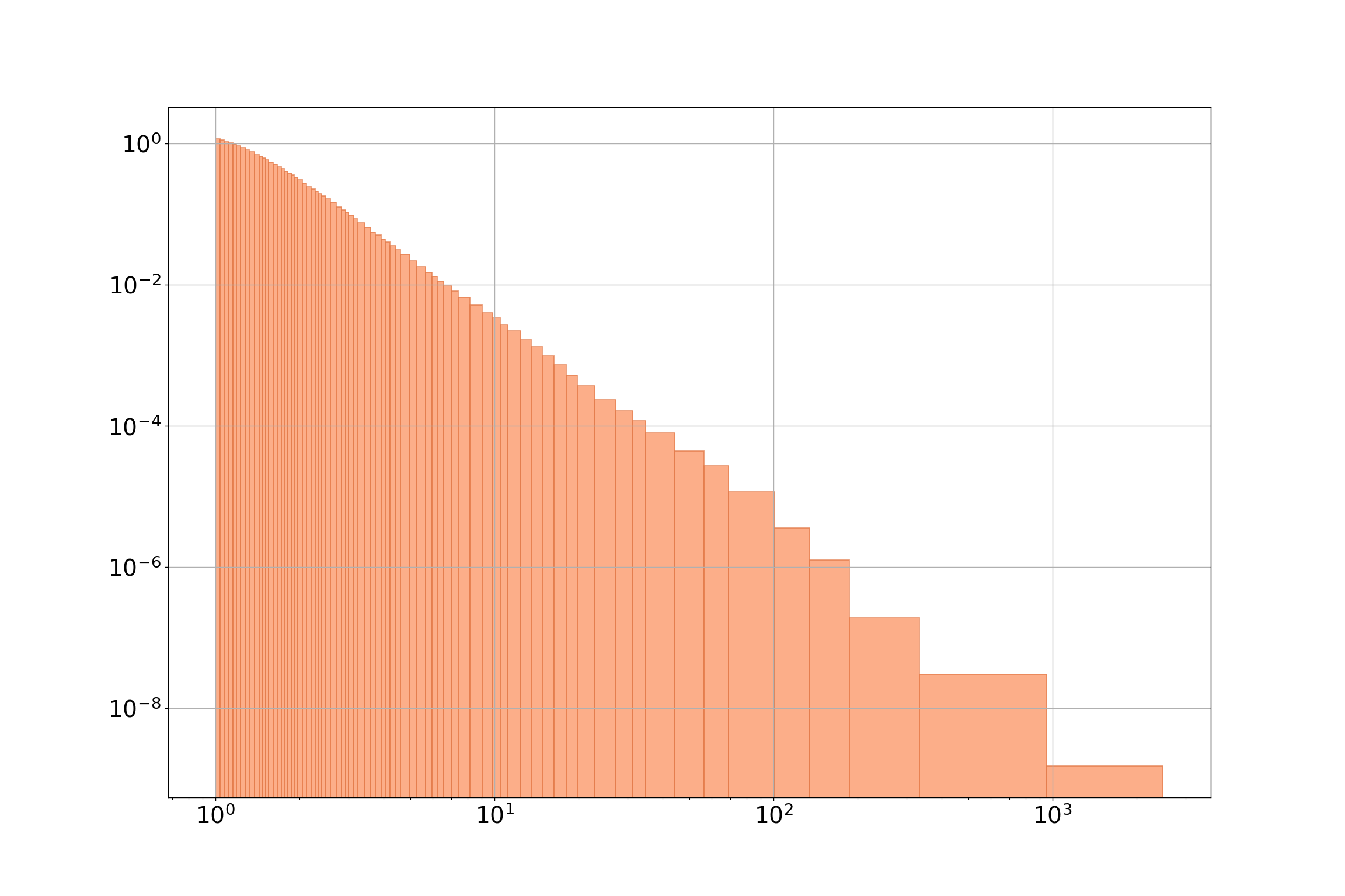
Figure 3: G-Enum histogram of the Lunar crater data set in a log scale ($K^{*}=75$)

Overall, the shape of our irregular histogram also shows that our approach can capture a power law decrease of the densities. This is in line with astrophysics literature: power or multiple power laws are often used to fit the crater size distribution (Wang and Zhou, 2016; Minton et al., 2019). The same information would be hard to convey with an equal-width histogram and an arbitrary number of bins. Our irregular histogram reveals interesting patterns and only requires a reasonable number of intervals to do so.

The density estimation experiment on this data set also shows the scalability of our method: the granular histogram was computed in about $1.3$ seconds. The taut-string method and the RMG approach remain usable with respectively about 54 seconds and 37 seconds, but both NML histogram ($\approx 17$ minutes of calculation) and the Bayesian Blocks method (almost 1 hour and 15 minutes of run time) use an unreasonable quantity of computational resources.

Figure 4: Different histograms obtained for the Lunar data set

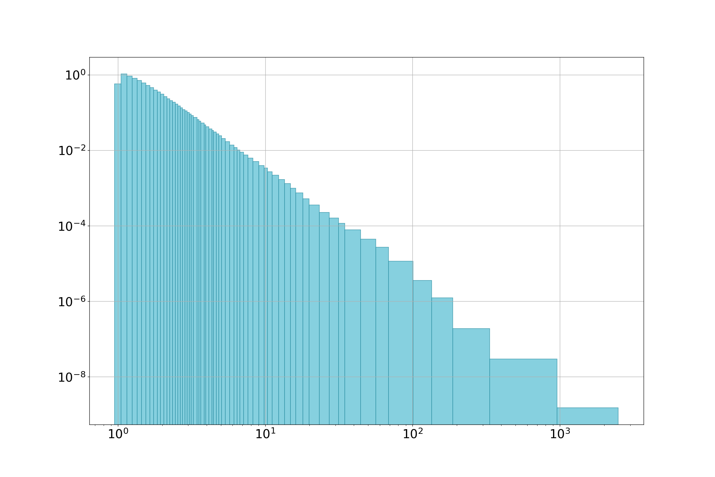
(a) NML + heuristic ($K^{*}=65$)

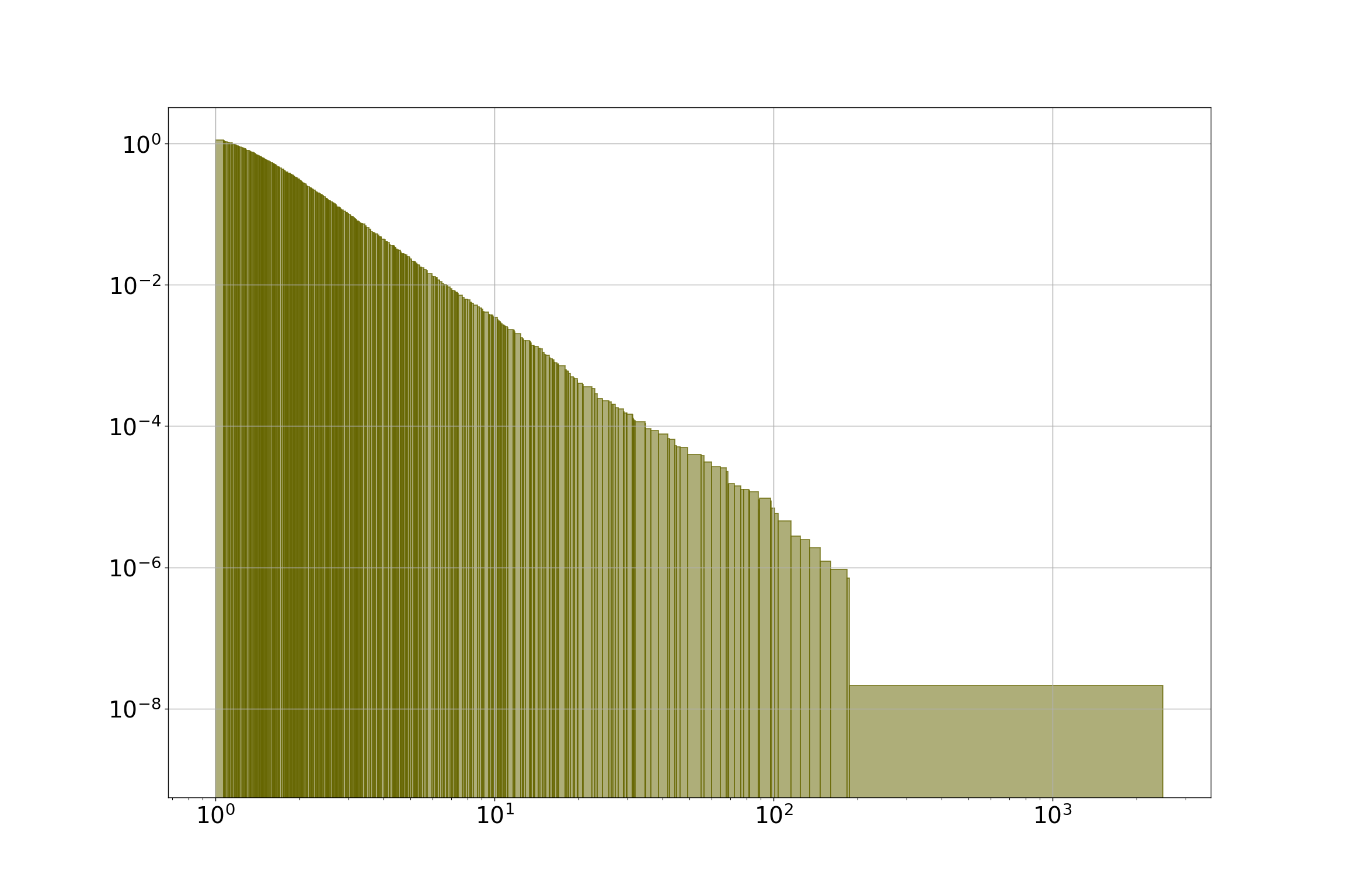
(b) Taut string ($K^{*}=478$)

(c) RMG ($K^{*}=73$)

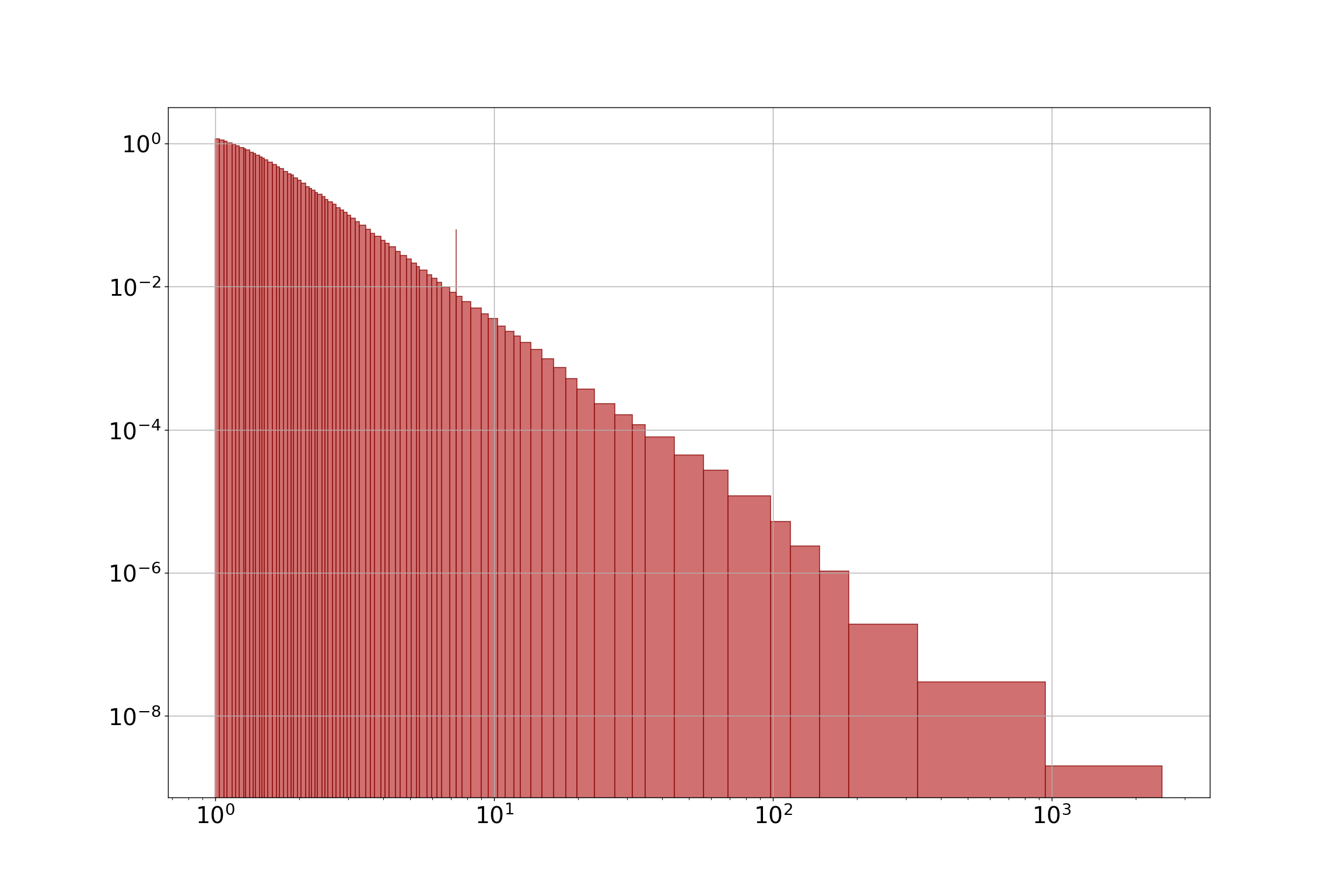
(d) Bayesian Blocks ($K^{*}=86$)

Figure 4 displays the histograms obtained by those methods while Table 10 gives the Hellinger distances between the densities estimated by the different methods. The NML histogram is the most unique one. The log log display used on the figures hides to some extent the main source of disagreement between the histograms which is the shorter first interval used by the NML histogram compared to the others. All other histograms are fairly close to one another. This emphasizes the non-parsimonious nature of the Taut string method which uses 478 intervals to produce an histogram that is fairly close to the one obtained by the Bayesian Blocks method with only 86 intervals. In addition, while this does not play a major role in the Hellinger distance because of its quite low support, the estimation of the tail of the distribution by the Taut string histogram seems to be more crude than other solutions.

Method	G-Enum	NML	RMG	TS	BB
G-Enum	-	0.131	0.0118	0.0103	0.0112
NML	-	-	0.131	0.123	0.130
RMG	-	-	-	0.0106	0.0114
TS	-	-	-	-	0.00846

Table 10: Hellinger distances between the densities estimated by the methods on the Lunar Crater data set.

Overall, this experiment confirms the computational efficiency of G-Enum and its ability to produce compact representations of complex and unknown distributions. Importantly, the resulting models are better or comparable to the ones obtained by less efficient solutions. G-Enum histograms provide interesting insights on the previously unknown distribution laws of large data sets without needing much computation time.

9 Conclusion

We presented a simple yet robust and very efficient enumerative criterion for histogram model selection that produces indistinguishable results to those obtained with much more compute-costly NML approach presented in a previous work.

By pairing our criterion with a search heuristic rather than the optimal but costly original optimisation algorithm, we achieve substantial gains in computation time. By introducing granularity to alleviate our dependency to the sole user parameter of this problem, the approximation accuracy $\epsilon$, we achieve substantial gains in robustness.

With our theoretical and experimental evaluation of these criteria we show that our granulated MDL criterion fills a gap in the current histogram model selection landscape : it’s a resilient, efficient and fully automated approach to histogram density estimation that can scale to explore known or unknown distribution laws in large data sets.

Appendix A Rewrite of K&M’s NML criterion

The final form of K&M’s NML criterion in their paper is as follows.

$$B(x^{n}|E,K,C) =\mathcal{SC}(x^{n}|\mathcal{M})+\log\binom{E}{K-1}$$

$$=\sum^{K}_{k=1}-h_{k}(\log(\epsilon\cdot h_{k})-\log(L_{k}\cdot n))$$

$$+\log\leavevmode\nobreak\ {\mathcal{R}}^{n}_{\mathcal{M}}+\log\binom{E}{K-1}$$

To ease the comparison of both criteria, we simplified the likelihood term as described heareafter.

$$\sum^{K}_{k=1}-h_{k}(\log(\epsilon\cdot h_{k})-\log(L_{k}\cdot n)) =\sum^{K}_{k=1}-h_{k}\left[\log\epsilon-\log L_{k}\right]$$

$$+\sum^{K}_{k=1}-h_{k}\left[\log h_{k}-\log n\right]$$

Then, we have

$$\sum^{K}_{k=1}-h_{k}\left[\log h_{k}-\log n\right] =-\log\left(\prod^{K}_{k=1}{h_{k}}^{h_{k}}\right)+\log n^{n}$$

$$=\log\frac{n^{n}}{{h_{1}}^{h_{1}}\dotsm{h_{K}}^{h_{K}}}$$

And

$$\sum^{K}_{k=1}-h_{k}\left[\log\epsilon-\log L_{k}\right]=\sum^{K}_{k=1}h_{k}\log\frac{L_{k}}{\epsilon}=\sum^{K}_{k=1}h_{k}\log E_{k}$$

Appendix B Proofs

Proofs are not given in the same order as in the main text. Indeed proofs of propositions 5 and 6 are based on proposition 8 but for the clarity of exposure, we preferred to present this latter proposition before the former ones. Of course, the proof of proposition 8 uses neither proposition 5 nor proposition 6, which is emphasized by the natural mathematical order used in the present section.

B.1 Proof of proposition 1

Proposition 1.

Let $\mathcal{M}=(K,(c_{k})_{0\leq k\leq K},(h_{k})_{1\leq k\leq K})$ be an optimal histogram for the data set $D$. Then

$$\forall k,1\leq k\leq K\ c_{k-1}<c_{k}.$$

In other words, an optimal histogram cannot contain zero-length intervals.

Proof.

Let $\mathcal{M}=(K,(c_{k})_{0\leq k\leq K},(h_{k})_{1\leq k\leq K})$ be a histogram compatible with $D$. Let us assume that $c_{l-1}=c_{l}$ for some $l>0$ and let $\mathcal{M^{\prime}}=(K-1,(c^{\prime}_{k})_{0\leq k\leq K-1},(h_{k}^{\prime})_{1\leq k>K})$ be the histogram derived from $\mathcal{M}$ by removing the zero-length interval. It is defined formally by

$$c^{\prime}_{k}=\begin{cases}c_{k}&\text{when }k<l\\ c_{k+1}&\text{when }k\geq l,\end{cases}$$

and

$$h^{\prime}_{k}=\begin{cases}h_{k}&\text{when }k<l\\ h_{k+1}&\text{when }k\geq l.\end{cases}$$

Obviously, $\mathcal{M^{\prime}}$ defines the same density as $\mathcal{M}$. In addition, as $h_{l}=0$

$$\sum^{K}_{k=1}h_{k}\log E_{k} =\sum^{K}_{k=1,k\neq l}h_{k}\log E_{k},$$

$$=\sum^{K}_{k=1,k\neq l}h_{k}\log\frac{c_{k}-c_{k-1}}{\epsilon},$$

$$=\sum^{K-1}_{k=1}h^{\prime}_{k}\log\frac{c^{\prime}_{k}-c^{\prime}_{k-1}}{\epsilon}, =\sum^{K-1}_{k=1}h^{\prime}_{k}\log E^{\prime}_{k}.,$$

and

$$\log\frac{n!}{\prod_{k=1}^{K}h_{k}!} =\log\frac{n!}{\prod_{k=1,k\neq l}^{K}h_{k}!},$$

$$=\log\frac{n!}{\prod_{k=1}^{K-1}h^{\prime}_{k}!}.$$

Therefore $\Delta=c_{\leavevmode\nobreak\ \textnormal{Enum}}(\mathcal{M}|D)-c_{\leavevmode\nobreak\ \textnormal{Enum}}(\mathcal{M^{\prime}}|D)$ is given by

$$\Delta= \log^{*}K-\log^{*}(K-1)$$

$$+\log\binom{E+K-1}{K-1}-\log\binom{E+K-2}{K-2}$$

$$+\log\binom{n+K-1}{K-1}-\log\binom{n+K-2}{K-2},$$

which shows that $\Delta>0$ and thus that $\mathcal{M}$ cannot be optimal. ∎

B.2 Proof of proposition 2

Proposition 2.

Let $D$ be a data set with $n$ observations. Let us denote $\mathcal{M}_{K=n}$ a histogram compatible with $D$ such that there is one observation per interval and $\mathcal{M}_{K=1}$ a histogram compatible with $D$ with only one interval. Then the coding length of $\mathcal{M}_{K=1}$ is shorter than the one of $\mathcal{M}_{K=n}$:

$$c_{\leavevmode\nobreak\ \textnormal{Enum}}(\mathcal{M}_{K=n}|D)>c_{\leavevmode\nobreak\ \textnormal{Enum}}(\mathcal{M}_{K=1}|D).$$

Proof.

If $\mathcal{M}_{K=n}$ is compatible with $D$ and there is one observation per interval, then $\forall k,h_{k}=1$ and obviously, $E>n$. Also $\forall k,E_{k}>0$.

Let us define

$$\delta c_{\leavevmode\nobreak\ \textnormal{Enum}}(n,1)=c_{\leavevmode\nobreak\ \textnormal{Enum}}(\mathcal{M}_{K=n})-c_{\leavevmode\nobreak\ \textnormal{Enum}}(\mathcal{M}_{K=1}).$$

Then we have

$$\delta c_{\leavevmode\nobreak\ \textnormal{Enum}}(n,1) = \log\binom{E+n-1}{n-1}+\log\binom{2n-1}{n-1}$$

$$+\log n!+\sum^{n}_{k=1}\log E_{k}$$

$$+\log^{*}n-\log^{*}1-n\log E.$$

Since $\log\binom{E+n-1}{n-1}=\sum^{n-1}_{k=1}{\log(E+k)}-\log(n-1)!$, we get

$$\delta c_{\leavevmode\nobreak\ \textnormal{Enum}}(n,1) = \sum^{n-1}_{k=1}{\log(E+k)}+\log\binom{2n-1}{n-1}$$

$$+\log n+\sum^{n}_{k=1}\log E_{k}$$

$$+\log^{*}n-\log^{*}1-n\log E.$$

As function $f(x)=\log(1+x)$ is strictly concave and $f(0)=0$, it is sub-additive on $[0,+\infty[$. We obtain

$$\sum^{n}_{k=1}\log E_{k} = \sum^{n}_{k=1}f(E_{k}-1)$$

$$\geq f\left(\sum^{n}_{k=1}(E_{k}-1)\right)$$

$$\geq \log(E-n+1).$$

Back to $\delta c_{\leavevmode\nobreak\ \textnormal{Enum}}(n,1)$, we get

$$\delta c_{\leavevmode\nobreak\ \textnormal{Enum}}(n,1) \geq \sum^{n-1}_{k=1}{\log E(1+\frac{k}{E})}+\log\binom{2n-1}{n-1}$$

$$\log n+\log E(1-\frac{n-1}{E})$$

$$+\log^{*}n-\log^{*}1-n\log E$$

$$\geq \log^{*}n-\log^{*}1+\log n+\log\binom{2n-1}{n-1}$$

$$+\sum^{n-1}_{k=1}{\log(1+\frac{k}{E})}+\log(1-\frac{n-1}{E}).$$

As $n\leq E$, we get

$$\log(1-\frac{n-1}{E})+\log n = \log(n-\frac{n}{E}(n-1))$$

$$\geq \log(n-(n-1))$$

$$\geq 0.$$

Finally, $\delta c_{\leavevmode\nobreak\ \textnormal{Enum}}(n,1)>0$, which proves the claim that the histogram with one single interval is always more probable than the one with $n$ singleton intervals. ∎

B.3 Proof of proposition 3

Proposition 3.

Let $D$ be a data set with $n$ observations. Let us denote $\mathcal{M}_{K>n}$ a histogram compatible with $D$ consisting of either singleton or empty intervals, one interval for each observation and empty intervals in-between, and let $\mathcal{M}_{K=1}$ be as in Proposition 2. Then the coding length of $\mathcal{M}_{K=1}$ is shorter than the one of $\mathcal{M}_{K>n}$:

$$c_{\leavevmode\nobreak\ \textnormal{Enum}}(\mathcal{M}_{K>n}|D)>c_{\leavevmode\nobreak\ \textnormal{Enum}}(\mathcal{M}_{K=1}|D).$$

Proof.

Let us consider a histogram consists with $K>n$ intervals composed of $E_{k}$ $\epsilon$-bins, with either $h_{k}=1$ for the singleton intervals and $h_{k}=0$ for the empty intervals.

$$\delta c_{\leavevmode\nobreak\ \textnormal{Enum}}(K,1) = \log\binom{E+K-1}{K-1}+\log\binom{n+K-1}{K-1}$$

$$+\log^{*}K-\log^{*}1+\log n!$$

$$+\sum^{n}_{k=1}\log E_{k}-n\log E.$$

We have

$$\log\binom{E+K-1}{K-1} = \sum^{K-1}_{k=1}{\frac{\log(E+k)}{\log k}}$$

$$= \sum^{n}_{k=1}{\frac{\log(E+k)}{\log k}}$$

$$+\sum^{K-1}_{k=n+1}{\frac{\log(E+k)}{\log k}}$$

Given that $\log(E+k)>\log E$, we have $\sum^{n}_{k=1}{\frac{\log(E+k)}{\log k}}>n\log E-\log n!$. Likewise, we know that $\log(E+k)>\log k$, so the sum $\sum^{K-1}_{k=n+1}{\frac{\log(E+k)}{\log k}}$ is greater than $\sum^{K-1}_{k=n+1}{1}=K-n-1$. Given these two lower bounds, we can write that

$$\log\binom{E+K-1}{K-1}>n\log E-\log n!+(K-n-1)$$

We then obtain

$$\delta c_{\leavevmode\nobreak\ \textnormal{Enum}}(K,1) > (K-n-1)$$

$$+\log\binom{n+K-1}{K-1}$$

$$+\log^{*}K-\log^{*}1+\sum^{n}_{k=1}\log E_{k}.$$

Finally, $\delta c_{\leavevmode\nobreak\ \textnormal{Enum}}(K,1)>0$, which proves the claim that the histogram with one single interval is more probable that any histogram where entries are in singleton intervals.

∎

Note 1.

Similar results to Proposition 2 and Proposition 3 could not be obtained for the NML criterion given by equation (3) for two reasons. First, the analysis of the criterion for histograms with $K$ singleton intervals ($n\leq K\leq E$) is complex, since the prior term $\log\binom{E}{K-1}$ is not monotonous and decreases for $K>E/2$. Second, the parametric complexity $\log\mathcal{R}^{n}_{\mathcal{M}_{K}}$ term has no closed-form formula and its best known approximations (Kontkanen, 2009; Szpankowski, 1998) are given for fixed $K$ as $n$ goes to infinity. These approximations cannot be used when $n\leq K\leq E$.

B.4 Proof of proposition 4

We begin by evaluating the expression of the cost variation $\Delta c$ after the merge of two intervals. Let A and B be two adjacent intervals composed of $E_{A}$, $E_{B}$ $\epsilon$-length elementary bins and of data counts $h_{A}$, $h_{B}$ in a $K$-bin histogram. They are merged into a single interval composed of $E_{A\cup B}=E_{A}+E_{B}$ $\epsilon$-length elementary bins with $h_{A\cup B}=h_{A}+h_{B}$ elements, creating a histogram with $K-1$ bins (we consider only histograms compatible with the data).

For this fusion, the variation for the Enum criterion, $\Delta c$, is given by

$${\Delta c_{\leavevmode\nobreak\ \textnormal{Enum}}}= c_{\leavevmode\nobreak\ \textnormal{Enum}}(\mathcal{M}_{K-1})-c_{\leavevmode\nobreak\ \textnormal{Enum}}(\mathcal{M}_{K})$$ (15)

$$= \log\frac{K-1}{E+K}+\log\frac{K-1}{n+K-1}$$

$$+\log^{*}(K-1)-\log^{*}K$$

$$+\log\frac{h_{A}!h_{B}!}{(h_{A}+h_{B})!}+\log\frac{(E_{A}+E_{B})^{(h_{A}+h_{B})}}{{E_{A}}^{h_{A}}\cdot{E_{B}}^{h_{B}}}$$

The fusion of two intervals is advantageous if the code length for the histogram with $K-1$ intervals is smaller than the code length for the histogram with $K$ intervals, that is if $\Delta c_{\leavevmode\nobreak\ \textnormal{Enum}}<0$. Proposition 4 corresponds to an interesting particular case.

Proposition 4.

The coding length of a histogram with two adjacent empty intervals is always longer than the coding length of a histogram with no consecutive empty intervals.

Proof.

We analyse the cost variation when two adjacent intervals are empty for the Enum criterion ($h_{A}=0$, $h_{B}=0$, so $h_{A}+h_{B}=0$). From equation 15 we have

$${\Delta c_{\leavevmode\nobreak\ \textnormal{Enum}}} {}_{(h_{A}=0,h_{B}=0)}=$$

$$\log\frac{K-1}{E+K-1}+\log\frac{K-1}{n+K-1}$$

$$+\log^{*}(K-1)-\log^{*}K$$

Given that $n+K-1>K-1$, we have  $\log\frac{K-1}{n+K-1}<0$. Similarly, $E+K-1>K-1$, so  $\log\frac{K-1}{E+K-1}<0$. Rissanen’s universal code for integers ($\log^{*}K$) is a monotone function, so $\log^{*}K-1-\log^{*}K<0$.

We have thus shown that, for the Enum criterion, the cost variation is always strictly negative after the merge of two adjacent empty intervals. This means that keeping a model with two adjacent empty bins is always more costly in terms of code length, so our search algorithm will systematically favor the merge of two consecutive empty bins. ∎

B.5 Proof of proposition 7

Proposition 5.

An optimal histogram has at most $2n-2$ intervals ($K^{*}\leq 2n-2$).

Proof.

The maximal number of non empty intervals is obviously bounded by the number of observations $n$. Provided the data set has $n$ distinct observations and that $\epsilon$ is small enough, we can consider a histogram with $n$ intervals containing each a single observation, separated by empty intervals. According to proposition 6 an optimal histogram cannot have consecutive empty intervals and thus the maximal number of separating intervals is $n-1$. Therefore an optimal histogram cannot have more than $2n-1$ intervals.

But proposition 3 shows that a histogram with a single interval is preferred by the criterion over a histogram consisting only of empty intervals and intervals containing each a single observation. Therefore the maximal model with $2n-1$ intervals cannot be optimal. Then the optimal number of intervals $K^{*}$ is bounded by $2n-2$. ∎

B.6 Proof of proposition 8

Proposition 8.

In an optimal histogram, each endpoint is at most $\epsilon$ away from one of the values of the data set.

Proof.

Let $\mathcal{M}^{\star}=(K,\{c_{k}\}_{0\leq k\leq K},\{h_{k}\}_{1\leq k\leq K})$ be an optimal histogram built from a data set $D$.

As by definition, $c_{0}=x_{min}-\epsilon/2$ and $c_{K}=x_{max}+\epsilon/2$, the property is valid for $c_{0}$ and $c_{K}$.

Let us now assume that $K>1$ and focus on endpoints $c_{k},0<k<K$, that is on cut-points between adjacent intervals.

Let $i,j=i+1$ be the index of two such adjacent intervals. We study the location of the cut-point between intervals $i$ and $j$, $c_{i}$, while considering the exterior boundaries of intervals $i$ and $j$ ($c_{i-1}$ and $c_{j}$) to be fixed. We denote $L_{i,j}=c_{j}-c_{i-1}$. We consider also the data counts of the intervals $h_{i}$ and $h_{j}$ to be fixed. In other words, we study to what extent the cut-point between intervals $i$ and $j$ can be freely set at grid positions in the empty space between the last data point in $i$ and the first data point in $j$, as illustrated by Figure 5.

Let $D_{i}$ (resp $D_{j}$) be the data point in interval $i$ (resp. $j$). We define

$$L_{i}=\min\{t\epsilon\mid\max D_{i}\leq c_{i-1}+t\epsilon\},$$

and

$$L_{j}=\min\{t\epsilon\mid\min D_{j}>c_{j}-t\epsilon\},$$

i.e. $L_{i}$ and $L_{j}$ are the minimum lengths of intervals that contain respectively $D_{i}$ and $D_{j}$.

In terms of elementary $\epsilon$-length bins, let $E_{i}=L_{i}/\epsilon,E_{j}=L_{j}/\epsilon,\widehat{E}=L_{i,j}/\epsilon$. We note $x=l/\epsilon\in[0,\widehat{E}-E_{i}-E_{j}]$ the number of $\epsilon$-length bins at which the cut-point $c_{i}$ is placed.

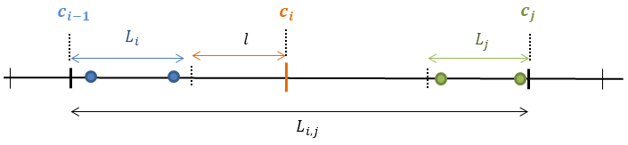
Figure 5: Illustration and notations of the optimal cut-point between two values problem

In this setting, each different value of $x$ defines a different $K$-bin histogram, $\mathcal{M}_{K}(x)$. Using the Enum criterion, each model has the following cost :

$$c_{\leavevmode\nobreak\ \textnormal{Enum}}(\mathcal{M}_{K}(x)|D)= \log\binom{E+K-1}{K-1}+\log\binom{n+K-1}{K-1}$$

$$+\log^{*}K+\log\frac{n!}{h_{1}!\ldots h_{i}!h_{j}!\ldots h_{K}!}$$

$$+\sum_{k<i}{h_{k}\log E_{k}}+h_{i}\log(E_{i}+x)$$

$$+h_{j}\log(\widehat{E}-(E_{i}+x))+\sum_{k>j}{h_{k}\log E_{k}}$$

Seeing as we focus on the frontier between just two intervals, the model index term does not change. Since the data counts of each interval are preserved regardless of the position of the interval’s endpoints, the corresponding part of the likelihood term will not change. In this setting, the sole term responsible for the cost variation between models is:

$$f_{h_{i},h_{j}}(x)=h_{i}\log(E_{i}+x)+h_{j}\log(\widehat{E}-(E_{i}+x))$$

From Proposition 4, an optimal histogram cannot contain two consecutive empty intervals, therefore at least one of the two intervals is non empty. We study the three possible cases.

1. Let us first consider the case where both intervals are non empty ($h_{i}>0$ and $h_{j}>0$). As $f_{h_{i},h_{j}}$ is a concave function on the closed interval $[0,\widehat{E}-E_{i}-E_{j}]$, its minimum values are only reached at its extremities, that is for $x=0$ and $x=\widehat{E}-E_{i}-E_{j}$.

   We have thus shown that the best cut-point between the two intervals is placed at at most $\epsilon$, either from last value of the first interval or from the first value of the second interval.

2. Let us now consider the case where the first interval is non empty, that is $h_{i}>0$ and $h_{j}=0$. Then $f_{h_{i},h_{j}}(x)=h_{i}\log(E_{i}+x)$. In this case, the minimum value of $f_{h_{i},h_{j}}(x)$ is obtained for $x=0$, that is with a cut-point placed at at most $\epsilon$ from last value of the first interval.

3. Similarly, if the second interval is non empty, the cut-point is placed at at most $\epsilon$ from the first value of the second interval. Let us notice that in both cases, the empty interval is of maximal length.

Overall, the endpoints of the optimal histogram are always at at most $\epsilon$ from one value of the data set. ∎

Note 2.

Intuitively, the choice of which one of these two placements is best will also depend on the data count of each interval. As we have highlighted before, a part of the likelihood term will favour shorter dense intervals over large ones. See the proof of proposition 5 for an illustration in a simple case.

Note 3.

Notice that for any value $x(c_{k})$ of the data set that is the closest one from an endpoint $c_{k}$, $c_{k}$ is as close as possible from $x(c_{k})$. In particular, if $x(c_{k})$ is the last point in the interval $]c_{k-1},c_{k}]$, we have $c_{k}-x(c_{k})<\epsilon$ with a strict inequality. Otherwise, the interval $]c_{k-1},c_{k}-\epsilon]$ still contains $x(c_{k})$, with an endpoint closer from $x(c_{k})$.

Note 4.

Empty intervals are always as long as possible, with their two endpoints close to values of the data set.

B.7 Proof of proposition 5

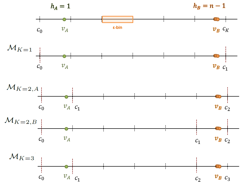
Figure 6: Graphical representation of the different cases involved in proposition 5.

Proposition 5.

There exist data sets such that the optimal histogram has at least one interval which contains only a single observation.

Proof.

Let us consider a data set with $n$ observations and only two distinct values $v_{A},v_{B}$ of frequencies $h_{A}=1,h_{B}=n-1$. We choose $v_{A}$ and $v_{B}$ such that $v_{B}-v_{A}\geq 3\epsilon$. According to proposition 4 an optimal histogram cannot contain successive empty intervals and thus we need only to consider three cases: histograms with one, two or three intervals. Those cases are illustrated on Figure 6.

For $K=1$, we have

$$c_{\leavevmode\nobreak\ \textnormal{Enum}}(\mathcal{M}_{K=1}) = n\log E+\log^{*}1.$$

For $K=2$, the optimal split is necessarily within $\epsilon$ of $v_{A}$ or $v_{B}$ according to proposition 8. If the split is close to $v_{A}$, we have $E_{A}=1,E_{B}=E-1$ and

$$c_{\leavevmode\nobreak\ \textnormal{Enum}}(\mathcal{M}_{K=2,A}) = \log^{*}2+\log(E+1)+\log(n+1)$$

$$+\log n+(n-1)\log(E-1)$$

$$= n\log E+o(n).$$

If the split is close to $v_{B}$, we have $E_{A}=E-1,E_{B}=1$ and

$$c_{\leavevmode\nobreak\ \textnormal{Enum}}(\mathcal{M}_{K=2,B}) = \log^{*}2+\log(E+1)+\log(n+1)$$

$$+\log n+\log(E-1)$$

$$= 2\log E+2\log n+O(1).$$

For $K=3$, the optimal split is necessarily right next to each value and we thus have two non-empty intervals composed $E_{A}=1,E_{B}=1$ $\epsilon$-bins, surrounding an empty interval of $E-2$ $\epsilon$-bins (this is again a consequence of proposition 8). We get

$$c_{\leavevmode\nobreak\ \textnormal{Enum}}(\mathcal{M}_{K=3}) = \log^{*}3+\log\frac{(E+1)(E+2)}{2}$$

$$+\log\frac{(n+1)(n+2)}{2}+\log n$$

$$= 2\log E+3\log n+O(1).$$

Therefore, even for rather small $n$ and $E$, the model cost is minimal for $K=2$ with the split within $\epsilon$ from $v_{B}$, i.e. for the histogram where the first interval contains the singleton value $v_{A}$. ∎

B.8 Proof of proposition 6

Proposition 6.

There exist data sets such that the optimal histogram has at least one interval that does not contain any observation.

Proof.

Let us consider a data set with $n$ observations and only two values $v_{A},v_{B}$ of frequencies $h_{A}=h_{B}=\frac{n}{2}$. We choose $v_{A}$ and $v_{B}$ such that $v_{B}-v_{A}\geq 3\epsilon$. For the same reasons as in the proof of proposition 5 we need only to consider three cases: histograms with one, two or three intervals.

For $K=1$, we have

$$c_{\leavevmode\nobreak\ \textnormal{Enum}}(\mathcal{M}_{K=1}) = n\log E+\log^{*}1.$$

For $K=2$, the optimal split is necessarily within $\epsilon$ of $v_{A}$ or $v_{B}$ according to proposition 8. Because of the symmetry of the setting, we can set the split to be near $v_{B}$. Thus we have two intervals composed of $E_{A}=E-1,E_{B}=1$ $\epsilon$-bins.

We get

$$c_{\leavevmode\nobreak\ \textnormal{Enum}}(\mathcal{M}_{K=2}) = \log^{*}2+\log(E+1)+\log(n+1)$$

$$+\log\frac{n!}{h_{A}!h_{B}!}+h_{A}\log(E-1)$$

To analyse this quantity, we use the approximation given in Grunwald (2007) (formula 4.36) which states that for $\theta\in]0,1[$

$$\log{{n}\choose{\theta n}}=nH(\theta)-\frac{1}{2}\log(2\pi n\mathrm{var}(\theta))+O\left(\frac{1}{n}\right),$$

with $H(\theta)=-\theta\log\theta-(1-\theta)\log(1-\theta)$ and $\mathrm{var}(\theta)=\theta(1-\theta)$.

Using $h_{A}=h_{B}=\frac{1}{2}$, we obtain

$$\log\frac{n!}{h_{A}!h_{B}!}=n\log 2-\frac{1}{2}\log\left(\pi\frac{n}{2}\right)+O\left(\frac{1}{n}\right),$$

and thus

$$c_{\leavevmode\nobreak\ \textnormal{Enum}}(\mathcal{M}_{K=2})=n\log(2\sqrt{E})+\log E+\frac{1}{2}\log n+O(1).$$

Finally, as in the proof of proposition 5, the optimal histogram with $K=3$ intervals consists in two non-empty intervals, each with $E_{A}=1,E_{B}=1$ $\epsilon$-bins, surrounding an empty interval composed of $E-2$ $\epsilon$-bins. Therefore

$$c_{\leavevmode\nobreak\ \textnormal{Enum}}(\mathcal{M}_{K=3}) = \log^{*}3+\log\frac{(E+1)(E+2)}{2}$$

$$+\log\frac{(n+1)(n+2)}{2}$$

$$+\log\frac{n!}{h_{A}!h_{B}!}$$

$$= n\log 2+2\log E+\frac{3}{2}\log n+O(1).$$

Therefore, even for rather small $n$ and $E$, the model cost is minimal for $K=3$, for the histogram where the second interval is empty and has $(E-2)\cdot\epsilon$. ∎

Appendix C Asymptotic behaviour of the MODL criterion when $\epsilon\rightarrow 0$

C.1 proof of Theorem 1

Theorem 1.

Let $D$ be a data set with $n$ observations. There exists two positive values $C(D)$ and $E(D)$ that depends only on $D$ such that for all $\epsilon\leq E(D)$ for any optimal histogram $\mathcal{M}^{\star}$ have

$$\begin{split}\left|c_{\leavevmode\nobreak\ \textnormal{Enum}}(\mathcal{M}^{\star}|D)-\left\{K-1+n-S(\mathcal{M}^{\star},D)\right\}\log\frac{1}{\epsilon}\right|\\ \leq C(D).\end{split}$$ (16)

Proof.

Let $D$ be a fixed data set with $n$ observations. For any $\epsilon$ such that $\dfrac{L}{\epsilon}$ is an integer, $\mathcal{M}_{\epsilon}^{\star}=(K,(c_{k})_{0\leq k\leq K},(h_{k})_{1\leq k\leq K})$ be a optimal histogram constructed on the $E=\dfrac{L}{\epsilon}+1$ regular grid of $\epsilon$-bins. The Enum criterion for $\mathcal{M}_{\epsilon}^{\star}$ is given by:

$$c_{\leavevmode\nobreak\ \textnormal{Enum}}(\mathcal{M}_{\epsilon}^{\star}|D) = \log^{*}K+\log\binom{n+K-1}{K-1}$$

$$+\log\binom{E+K-1}{K-1}$$

$$+\log\frac{n!}{h_{1}!...h_{K}!}+\sum^{K}_{k=1}h_{k}\log E_{k,\epsilon},$$

where the $E_{k,\epsilon}$ are the sizes of the intervals expressed in terms of $\epsilon$-bins.

More precisely, let $c_{0,\epsilon},c_{1,\epsilon},\ldots,c_{K,\epsilon}$ be the end points of the $K$ intervals of $\mathcal{M}_{\epsilon}^{\star}$. By definition of the grid, we have

$$L_{k,\epsilon}=c_{k,\epsilon}-c_{k-1,\epsilon}=E_{k,\epsilon}\times\epsilon,1\leq k\leq K$$

and

$$L+\epsilon=c_{K_{\epsilon},\epsilon}-c_{0,\epsilon}=E\times\epsilon.$$

Using

$$\log\binom{E+K-1}{K-1}=\sum_{k=1}^{K-1}\log(E+k)-\log(K-1)!,$$

and the notations above, we have

$$c_{\leavevmode\nobreak\ \textnormal{Enum}}(\mathcal{M}_{\epsilon}^{\star}|D) = \log^{*}K+\log\binom{n+K-1}{K-1}$$

$$+\log\frac{n!}{h_{1}!...h_{K}!}-\log(K-1)!$$

$$+\sum_{k=1}^{K-1}\log\left(\frac{L}{\epsilon}+k+1\right)$$

$$+\sum^{K}_{k=1}{h_{k}\log\frac{L_{k,\epsilon}}{\epsilon}}.$$

Obviously, the main influence of $\epsilon$ on the criterion is through the last two terms. Let us first notice that $\forall k,\ 1\leq k\leq K-1$

$$\log\left(\frac{L}{\epsilon}+k+1\right)=\log\frac{1}{\epsilon}+\log(L+(k+1)\epsilon).$$

and thus

$$\sum_{k=1}^{K-1}\log\left(\frac{L}{\epsilon}+k+1\right)=\\ (K-1)\log\frac{1}{\epsilon}+\sum_{k=2}^{K}\log(L+k\epsilon).$$ (17)

To analyse the last term $\sum^{K}_{k=1}{h_{k}\log\frac{L_{k,\epsilon}}{\epsilon}}$, let us define $D_{k,\epsilon}$ by

$$D_{k,\epsilon}=\arg\min_{x\in D}|c_{k,\epsilon}-x|-\arg\min_{x\in D}|c_{k-1,\epsilon}-x|,$$

that is the distance between the data points that are the closest to the boundaries of interval $]c_{k-1,\epsilon},c_{k,\epsilon}]$. By definition, we have

$$|L_{k,\epsilon}-D_{k,\epsilon}|\leq\min_{x\in D}|c_{k,\epsilon}-x|+\min_{x\in D}|c_{k-1,\epsilon}-x|.$$

By proposition 8 we know that

$$\forall 0\leq k\leq K,\ \min_{x\in D}|c_{k,\epsilon}-x|\leq\epsilon,$$

as $\mathcal{M}_{\epsilon}^{\star}$ is optimal. This shows that

$$|L_{k,\epsilon}-D_{k,\epsilon}|\leq 2\epsilon.$$

Using $D_{k,\epsilon}$, we have

$$\sum^{K}_{k=1}h_{k}\log\frac{L_{k,\epsilon}}{\epsilon}=$$ (18)

$$\sum_{D_{k,\epsilon}=0}h_{k}\log\frac{L_{k,\epsilon}}{\epsilon}+\sum_{D_{k,\epsilon}>0}h_{k}\left(\log\frac{1}{\epsilon}+\log\frac{L_{k,\epsilon}}{D_{k,\epsilon}}+\log D_{k,\epsilon}\right).$$

Using equations (17) and (18), we can decompose the Enum criterion $c_{\leavevmode\nobreak\ \textnormal{Enum}}(\mathcal{M}_{\epsilon}^{\star}|D)$ into the sum of the following three terms:

$$c_{1}(\mathcal{M}_{\epsilon}^{\star}|D) = \log^{*}K+\log\binom{n+K-1}{K-1}$$

$$+\log\frac{n!}{h_{1}!...h_{K}!}-\log(K-1)!$$

$$+\sum_{D_{k,\epsilon}=0}h_{k}\log\frac{L_{k,\epsilon}}{\epsilon}$$

$$+\sum_{D_{k,\epsilon}>0}{h_{k}\log D_{k,\epsilon}},$$

$$c_{2}(\mathcal{M}_{\epsilon}^{\star}|D) = \sum_{k=2}^{K}{\log(L+k\epsilon)}+\sum_{D_{k,\epsilon}>0}{\log\frac{L_{k,\epsilon}}{D_{k,\epsilon}}}.$$

$$c_{3}(\mathcal{M}_{\epsilon}^{\star}|D) = (K-1)\log\frac{1}{\epsilon}+\sum_{D_{k,\epsilon}>0}{h_{k}\log\frac{1}{\epsilon}},$$

As $\mathcal{M}_{\epsilon}^{\star}$ is optimal, $K\leq 2n-2$ (proposition 7) and as a consequence $c_{1}(\mathcal{M}_{\epsilon}^{\star}|D)$ is upper and lower bounded by constants that depend only on the data set.

This is obviously the case of the terms $\log^{\star}K$, $\log\binom{n+K-1}{K-1}$ and $-\log(K-1)!$. The term $\log\frac{n!}{h_{1}!...h_{K}!}$ can take only a finite number of positive values for a fixed $n$ and any $K\leq 2n-2$ and is therefore bounded by the largest of those values. Moreover, when $D_{k,\epsilon}=0$, $\epsilon\leq L_{k,\epsilon}\leq 2\epsilon$ and thus

$$0\leq\sum_{D_{k,\epsilon}=0}h_{k}\log\frac{L_{k,\epsilon}}{\epsilon}\leq n\log 2.$$

It is also obvious that $D_{k,\epsilon}\leq L$ and thus

$$\sum_{D_{k,\epsilon}>0}{h_{k}\log D_{k,\epsilon}}\leq n\log L.$$

To lower bound this quantity, we introduce

$$D_{\min}=\min\{|x_{i}-x_{j}|\mid x_{i}\in D,x_{j}\in D,x_{i}\neq x_{j}\},$$ (19)

which depends only on the data set $D$ and is strictly positive (by hypothesis on $D$). By definition for all $k$ such that $D_{k,\epsilon}>0$, $D_{k,\epsilon}\geq D_{\min}$, and therefore

$$\sum_{D_{k,\epsilon}>0}{h_{k}\log D_{k,\epsilon}}\geq\min(\log D_{\min},0).$$

Thus there exists $C_{1}(D)\geq 0$ such that for all $\epsilon>0$, $-C_{1}(D)\leq c_{1}(\mathcal{M}_{\epsilon}^{\star}|D)\leq C_{1}(D)$.

The second term $c_{2}(\mathcal{M}_{\epsilon}^{\star}|D)$ can also be upper and lower bounded with a minimal condition on $\epsilon$. Indeed we have

$$(K-1)\log L\leq\sum_{k=2}^{K}{\log(L+k\epsilon)}\leq(K-1)\log(L+K\epsilon).$$

Assuming that $\epsilon\leq L$ and with $K\leq 2n-2$, we have

$$(2n-3)\log L\leq\sum_{k=2}^{K}{\log(L+k\epsilon)}\leq(2n-3)\left(\log L+\log(2n-1)\right).$$

We also have for $D_{k,\epsilon}>0$

$$\begin{array}[]{rcccl}-2\epsilon&\leq&L_{k,\epsilon}-D_{k,\epsilon}&\leq&2\epsilon\\ -2\dfrac{\epsilon}{D_{k,\epsilon}}&\leq&\dfrac{L_{k,\epsilon}}{D_{k,\epsilon}}-1&\leq&2\dfrac{\epsilon}{D_{k,\epsilon}}\\ 1-2\dfrac{\epsilon}{D_{k,\epsilon}}&\leq&\dfrac{L_{k,\epsilon}}{D_{k,\epsilon}}&\leq&1+2\dfrac{\epsilon}{D_{k,\epsilon}}\\ 1-2\dfrac{\epsilon}{D_{\min}}&\leq&\dfrac{L_{k,\epsilon}}{D_{k,\epsilon}}&\leq&1+2\dfrac{\epsilon}{D_{\min}}\end{array}$$

Thus if we assume $\epsilon\leq\frac{D_{\min}}{4}<L$, we have

$$-\log 2\leq\log\left(\dfrac{L_{k,\epsilon}}{D_{k,\epsilon}}\right)\leq\log\frac{3}{2}.$$

Thus if $\epsilon\leq\frac{D_{\min}}{4}$, we have

$$\begin{array}[]{rcccl}-K\log 2&\leq&\displaystyle\sum_{D_{k,\epsilon}>0}{\log\frac{L_{k,\epsilon}}{D_{k,\epsilon}}}&\leq&K\log\frac{3}{2}\\ -(2n-2)\log 2&\leq&\displaystyle\sum_{D_{k,\epsilon}>0}{\log\frac{L_{k,\epsilon}}{D_{k,\epsilon}}}&\leq&(2n-2)\log\frac{3}{2}\end{array}$$

Thus there exists $C_{2}(D)\geq 0$ such that for all $K\leq 2|D|-2$ and for all $0<\epsilon\leq\frac{D_{\min}}{4}$, $-C_{2}(D)\leq c_{2}(\mathcal{M}_{\epsilon}^{\star}|D)\leq C_{2}(D)$.

The last term $c_{3}$ is the only one that depends on $\epsilon$ in a non bounded way. It can be interpreted in a more direct way using

$$\sum_{D_{k,\epsilon}>0}h_{k}=n-\sum_{D_{k,\epsilon}=0}h_{k},$$

and characterising intervals such that $h_{k}>0$ and $D_{k,\epsilon}=0$. Let $I_{k}$ be such an interval and let $x$ be a point from $D$ in $I_{k}$. When $D_{k,\epsilon}=0$, $L_{k,\epsilon}=\epsilon$ or $L_{k,\epsilon}=2\epsilon$. Combined with the assumption that $\epsilon\leq\frac{D_{\min}}{4}$, all data points in $I_{k}$ take the same value $x$.

Using proposition 8, we can then rule out the case $L_{k,\epsilon}=2\epsilon$. Indeed we have $I_{k}=]c_{k-1},c_{k}]$. According to proposition 8 both $c_{k-1}$ and $c_{k}$ must be at most distant of $\epsilon$ from a data point. Considering $D_{k,\epsilon}=0$ this must be the same value $x^{\prime}$. If $c_{k}-c_{k-1}=2\epsilon$, then the only possibility is that $c_{k}=x^{\prime}+\epsilon$ and $c_{k-1}=x^{\prime}-\epsilon$, and thus $x^{\prime}=x$, the only value taken by data points in $I_{k}$. However based on Remark 3 above, we should then have $c_{k}=x$. Thus, $L_{k,\epsilon}=\epsilon$ and $I_{k}$ is a singular interval as per definition 2. Therefore $\sum_{D_{k,\epsilon}=0}h_{k}=S(\mathcal{M}_{\epsilon}^{*},D)$, which concludes the proof. ∎

C.2 proof of Corollary 1

Corollary 1.

Let $D$ be a data set with $n$ distinct observations. Then for $\epsilon$ sufficiently small, the optimal histogram build on $\epsilon$ bins for the Enum criterion is the trivial one with a single interval

$$\mathcal{M}=(1,\{x_{\min}-\frac{\epsilon}{2},x_{\max}+\frac{\epsilon}{2}\},n).$$

Proof.

Let us consider two optimal histograms $\mathcal{M}_{K,\epsilon}^{\star}$ and $\mathcal{M}_{K^{\prime},\epsilon}^{\star}$ with $K\neq K^{\prime}$. We have

$$\bigl{|}c_{\leavevmode\nobreak\ \textnormal{Enum}}(\mathcal{M}_{K,\epsilon}^{\star}|D)-c_{\leavevmode\nobreak\ \textnormal{Enum}}(\mathcal{M}_{K^{\prime},\epsilon}^{\star}|D)-\\ \log\frac{1}{\epsilon}(K-K^{\prime}+S(\mathcal{M}_{K^{\prime},\epsilon}^{*},D)-S(\mathcal{M}_{K,\epsilon}^{*},D))\bigr{|}\leq 2C(D).$$

As $K$ (resp. $K^{\prime}$) and $S(\mathcal{M}_{K,\epsilon}^{*},D)$ (resp. $S(\mathcal{M}_{K^{\prime},\epsilon}^{*},D)$) are integers, the minimum non zero value of

$$|K-K^{\prime}+S(\mathcal{M}_{K^{\prime},\epsilon}^{*},D)-S(\mathcal{M}_{K,\epsilon}^{*},D)|$$

is 1. Therefore when $\epsilon<e^{-2C(D)}$, the sign of

$$c_{\leavevmode\nobreak\ \textnormal{Enum}}(\mathcal{M}_{K,\epsilon}^{\star}|D)-c_{\leavevmode\nobreak\ \textnormal{Enum}}(\mathcal{M}_{K^{\prime},\epsilon}^{\star}|D),$$

is the one of $K-K^{\prime}+S(\mathcal{M}_{K^{\prime},\epsilon}^{*},D)-S(\mathcal{M}_{K,\epsilon}^{*},D)$ as long as this quantity is not zero. In other words, histograms can be compared based on this difference as long as $\epsilon$ is small enough. Our goal is to show that $\mathcal{M}_{1,\epsilon}^{\star}$ is optimal. This histogram is preferred over $\mathcal{M}_{K,\epsilon}^{*}$ when

$$1-K+S(\mathcal{M}_{K,\epsilon}^{*},D)-S(\mathcal{M}_{1,\epsilon}^{*},D) <0,$$

$$S(\mathcal{M}_{K,\epsilon}^{*},D) <K-1,$$

as $\mathcal{M}_{1,\epsilon}^{\star}$ does not contain singular intervals.

Let us now focus on the assumption that the $n$ values in the data set are distinct. This implies that a singular interval $I_{k}$ is associated to $h_{k}=1$ and thus $S(\mathcal{M}_{K,\epsilon}^{*},D)$ is exactly the number of singular intervals. This number is controlled by the fact that when $\epsilon$ is small enough, a histogram cannot have adjacent singular intervals. Indeed singular intervals have a maximal width of $\epsilon$. Let $I_{k}$ and $I_{k+1}$ be two such adjacent intervals, with the associated values $x_{i}\in I_{k}$ and $x_{j}\in I_{j}$. Then

$$D_{\min}\leq|x_{j}-x_{i}|\leq 2\epsilon,$$

with $D_{\min}$ has defined in equation (19). The lower bound is induced by the fact that $I_{k}$ and $I_{k+1}$ contain only a single value each (by definition) and are adjacent: there is no value from the data set in $]x_{i},x_{j}[$. The inequalities can be fulfilled simultaneously only if $\epsilon\geq\frac{D_{\min}}{2}$ and thus when $\epsilon<\frac{D_{\min}}{2}$, singular intervals cannot be adjacent. We assume in the rest of the proof that $\epsilon<\min\left(\frac{D_{\min}}{2},e^{-2C(D)}\right)$. Then

$$K\geq 2S(\mathcal{M}_{K,\epsilon}^{*},D)-1,$$

as we need “in between” non singular intervals to separate singular ones. Therefore we have

$$K-S(\mathcal{M}_{K,\epsilon}^{*},D)\geq S(\mathcal{M}_{K,\epsilon}^{*},D)-1,$$

and if $S(\mathcal{M}_{K,\epsilon}^{*},D)\geq 3$,

$$S(\mathcal{M}_{K,\epsilon}^{*},D)\leq K-2.$$

This shows that $\mathcal{M}_{1,\epsilon}^{*}$ is always preferred to by the Enum criterion to histograms with $S(\mathcal{M}_{K,\epsilon}^{*},D)\geq 3$.

We need now to discuss the remaining cases, i.e., situations when $S(\mathcal{M}_{K,\epsilon}^{*},D)\leq 2$. If $K\geq S(\mathcal{M}_{K,\epsilon}^{*},D)+2$, $\mathcal{M}_{1,\epsilon}^{*}$ is preferred and thus we have two interesting particular cases to handle:

1. $K=2$ and $S(\mathcal{M}_{2,\epsilon}^{*},D)=1$: this is a particular case with a single singular interval completed by a single large non singular one;

2. $K=3$ and $S(\mathcal{M}_{3,\epsilon}^{*},D)=2$: this is again a particular case where we have two singular intervals separated by a single large non singular interval.

In both cases, the dominating term of the Enum criterion is $n\log\frac{1}{\epsilon}$, exactly as for $\mathcal{M}_{1,\epsilon}^{*}$ and we need to compare with more precision the values of the criterion to choose the optimal histogram.

For a single interval, we have

$$c_{\leavevmode\nobreak\ \textnormal{Enum}}(\mathcal{M}_{1,\epsilon}^{\star}|D)=\log^{*}1+n\log\left(\frac{L}{\epsilon}+1\right).$$ (20)

We use the fact that if $\lambda>0$, $\rho>0$ and $\kappa$ do not depend on $\epsilon$, for $\epsilon$ large enough such that $\frac{\rho}{\epsilon}+\kappa>0$,

$$\lambda\log\left(\frac{\rho}{\epsilon}+\kappa\right)=\lambda\log\rho+\lambda\log\frac{1}{\epsilon}+o(\epsilon).$$ (21)

Thus we have

$$c_{\leavevmode\nobreak\ \textnormal{Enum}}(\mathcal{M}_{1,\epsilon}^{\star}|D)=n\log\frac{1}{\epsilon}+\log^{*}1+n\log L+o(\epsilon).$$

For $K=2$ and $S(\mathcal{M}_{2,\epsilon}^{*},D)=1$, we have

$$c_{\leavevmode\nobreak\ \textnormal{Enum}}(\mathcal{M}_{2,\epsilon}^{\star})= \log^{*}2+\log(n+1)+\log n+\log\left(\frac{L}{\epsilon}+2\right)$$

$$+(n-1)\log\frac{L}{\epsilon}.$$

Using equation (21) to handle the two logarithmic terms with $\epsilon$, we have

$$c_{\leavevmode\nobreak\ \textnormal{Enum}}(\mathcal{M}_{2,\epsilon}^{\star}|D)= n\log\frac{1}{\epsilon}$$

$$+\log^{*}2+n\log L$$

$$+\log(n(n+1))+o(\epsilon).$$

Finally we have for $K=3$ and $S(\mathcal{M}_{2,\epsilon}^{*},D)=2$

$$c_{\leavevmode\nobreak\ \textnormal{Enum}}(\mathcal{M}_{3,\epsilon}^{\star}|D)= \log^{*}3+\log\frac{(n+1)(n+2)}{2}+$$

$$+\log\left(\frac{L}{\epsilon}+2\right)+\log\left(\frac{L}{\epsilon}+3\right)-\log 2$$

$$+(n-2)\log\left(\frac{L}{\epsilon}-1\right)$$

$$+\log n(n-1),$$

Using again equation (21), we have

$$c_{\leavevmode\nobreak\ \textnormal{Enum}}(\mathcal{M}_{3,\epsilon}^{\star}|D)= n\log\frac{1}{\epsilon}$$

$$+\log^{*}3+n\log L$$

$$+\log\frac{(n-1)n(n+1)(n+2)}{4}+o(\epsilon).$$

When $\epsilon$ converges to 0, $c_{\leavevmode\nobreak\ \textnormal{Enum}}(\mathcal{M}_{k,\epsilon}^{\star}|D)-n\log\frac{1}{\epsilon}-n\log L$ reduces to $\log^{\star}k$ plus some positive terms when $k>1$. As $\log^{\star}$ is an increasing function, when $\epsilon$ is mall enough, $c_{\leavevmode\nobreak\ \textnormal{Enum}}(\mathcal{M}_{1,\epsilon}^{\star}|D)$ becomes smaller than $c_{\leavevmode\nobreak\ \textnormal{Enum}}(\mathcal{M}_{k,\epsilon}^{\star}|D)$ for $k>1$ and thus $\mathcal{M}_{1,\epsilon}^{\star}$ is the optimal histogram. ∎

Appendix D Illustration of the asymptotic behaviour

We have:

$$c_{\leavevmode\nobreak\ \textnormal{Enum}}(\mathcal{M}_{2,\epsilon}|D_{n}(\alpha,\theta)) = \log^{*}2+\log(n+1)+\log(E+1)$$

$$+\log\frac{n!}{(n\theta)!(n(1-\theta))!}+n\theta\log\alpha E$$

$$+n(1-\theta)\log(1-\alpha)E,$$

$$= \log^{*}2+\log(n+1)+\log(E+1)$$

$$+nH(\theta)-\frac{1}{2}\log(2\pi n\mathrm{var}(\theta))+O(1/n)$$

$$+n\log E+n\theta\log\alpha$$

$$+n(1-\theta)\log(1-\alpha),$$

where we used the same approximation from Grunwald (2007) as in Section B.8. Using equation (20), we obtain

$$\Delta(n,\epsilon,\alpha,\theta)= c_{\leavevmode\nobreak\ \textnormal{Enum}}(\mathcal{M}^{\star}_{2,\epsilon}|D_{n}(\theta,\alpha))-c_{\leavevmode\nobreak\ \textnormal{Enum}}(\mathcal{M}^{\star}_{1,\epsilon}|D_{n}(\theta,\alpha))$$

$$= \log^{*}2-\log^{*}1+\log(n+1)+\log(E+1)$$

$$+nH(\theta)-\frac{1}{2}\log(2\pi n\mathrm{var}(\theta))+O(1/n)$$

$$+n\theta\log\alpha+n(1-\theta)\log(1-\alpha).$$

This can be simplified into

$$\Delta(n,\epsilon,\alpha,\theta)= \log\left(E+1\right)$$

$$+n\left(H(\theta)+\theta\log\alpha+(1-\theta)\log(1-\alpha)\right)$$

$$+O(\log n).$$

Finally we conclude using

$$D_{KL}(\theta\|\alpha) =\theta\log\frac{\theta}{\alpha}+(1-\theta)\log\frac{1-\theta}{1-\alpha},$$

$$=-H(\theta)-\theta\log\alpha-(1-\theta)\log(1-\alpha).$$

Appendix E Benchmarking and comparison of MDL methods

The first series of figures of the appendix compares the NML, Enum and G-Enum criteria. The three methods are evaluated on different sample sizes of a Normal (figure 7, Cauchy (figure 8), uniform (figure 9), triangle (figure 10), triangle mixture (figure 11) and Gaussia mixture (figure 12) distributions.

We highlight that all results are means over 10 experiments for each sample size. All results are shown in log scale. The standard deviations of the metrics are represented asymmetrically in the graphs to because of the log scale.

Figure 7: Comparison between MDL methods over a Normal distribution of different sample sizes

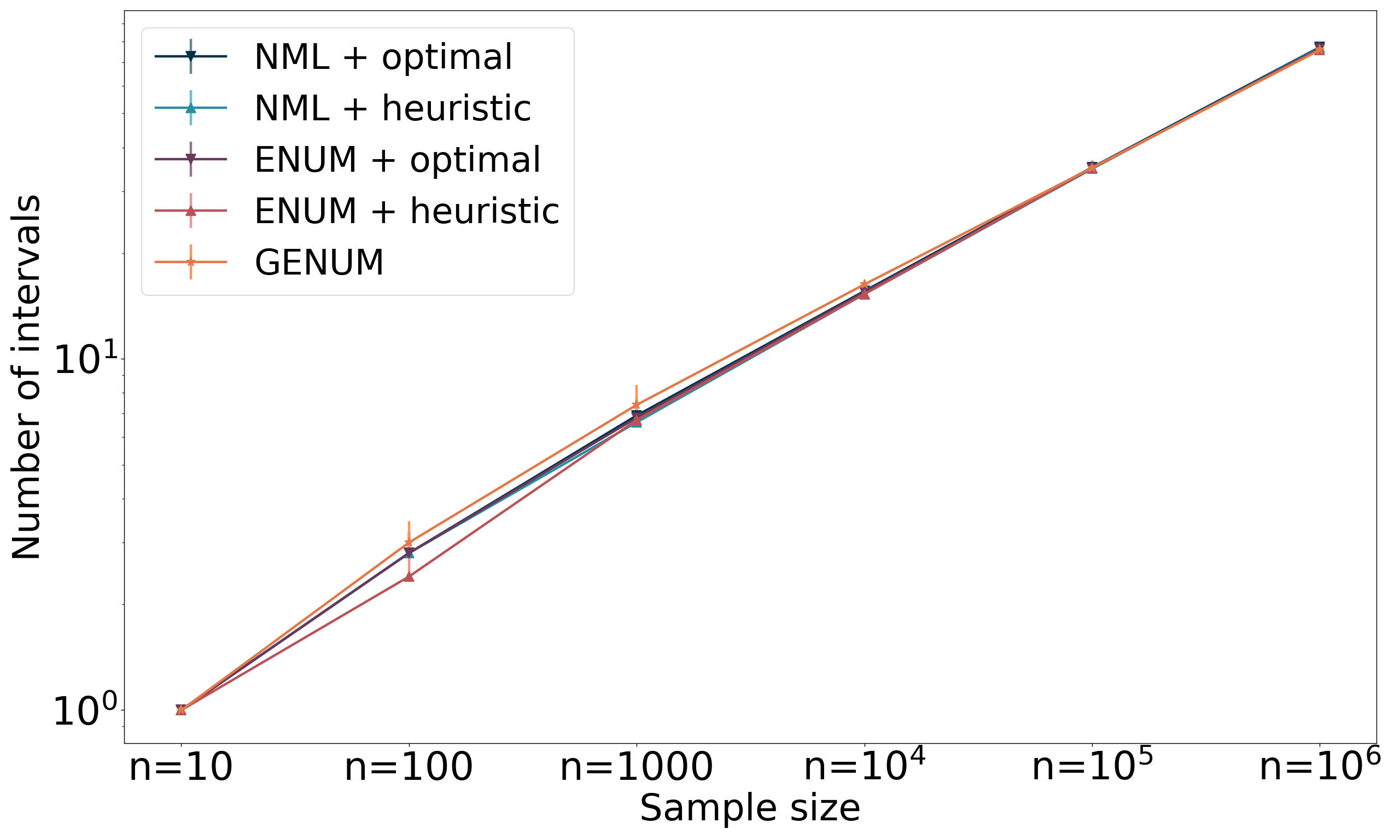
(a) Number of intervals,

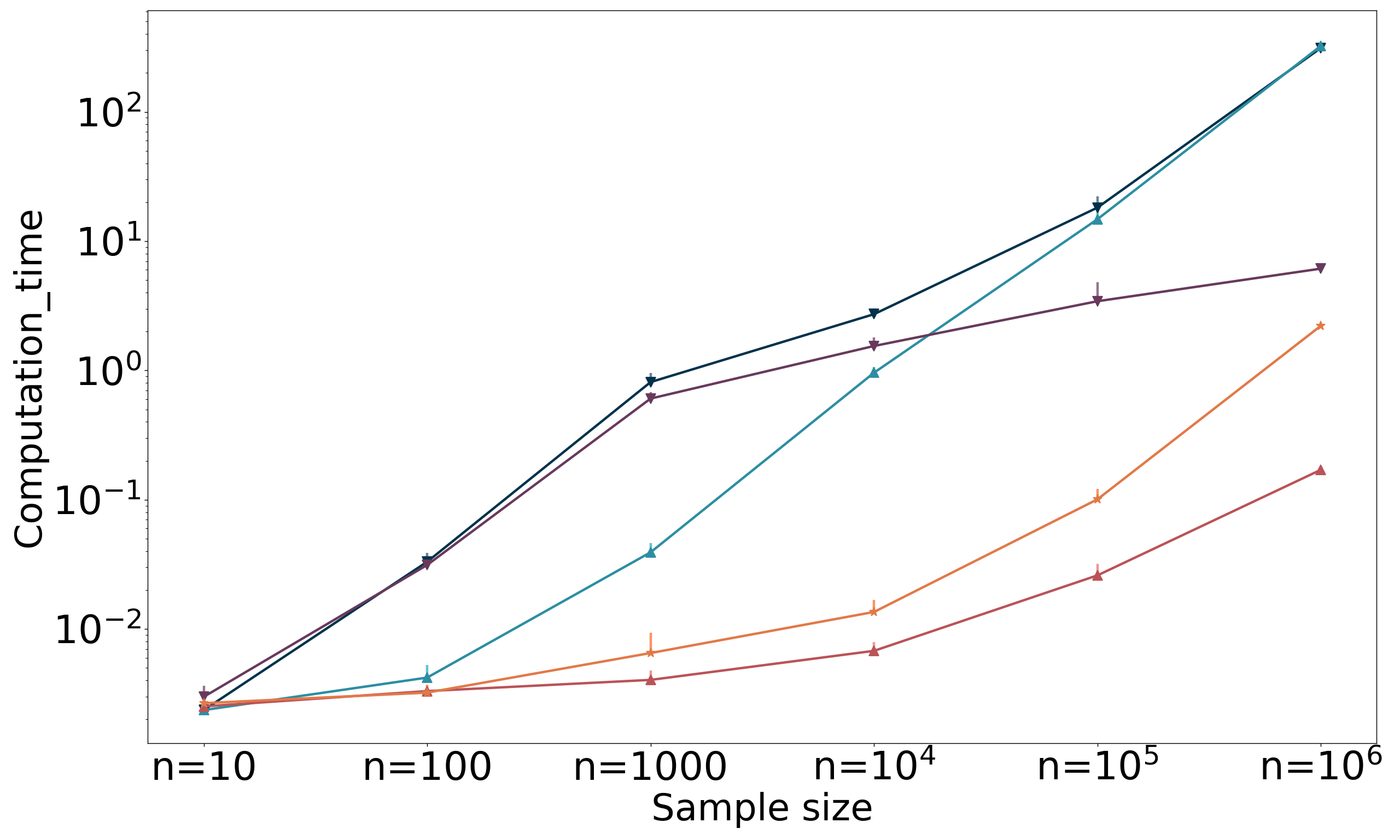
(b) Computation time,

(c) Hellinger distance,

Figure 8: Comparison between MDL methods over a Cauchy distribution of different sample size

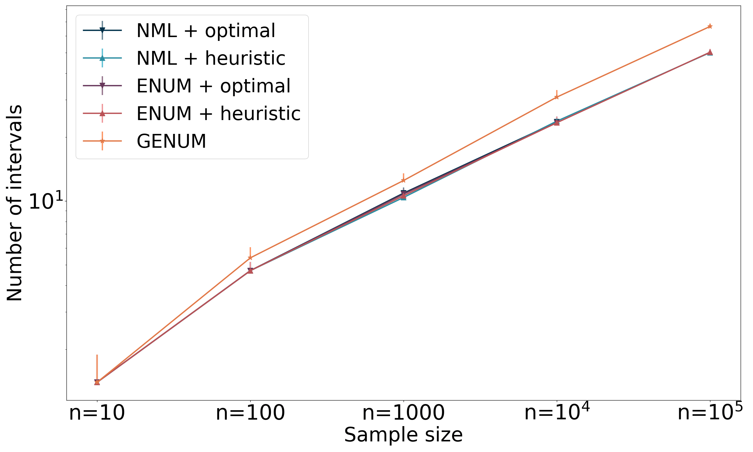
(a) Number of intervals,

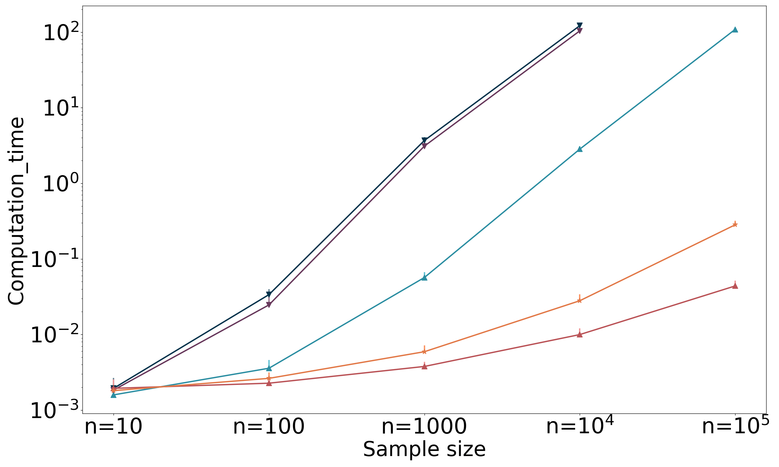
(b) Computation time,

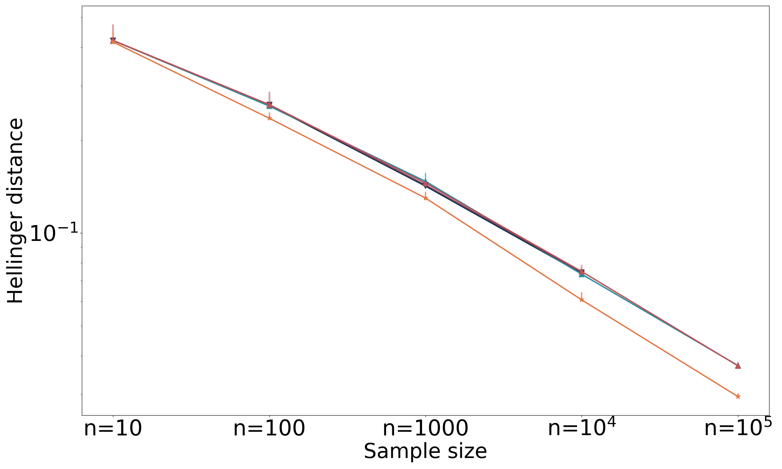
(c) Hellinger distance,

Figure 9: Comparison between MDL methods over a uniform distribution of different sample size

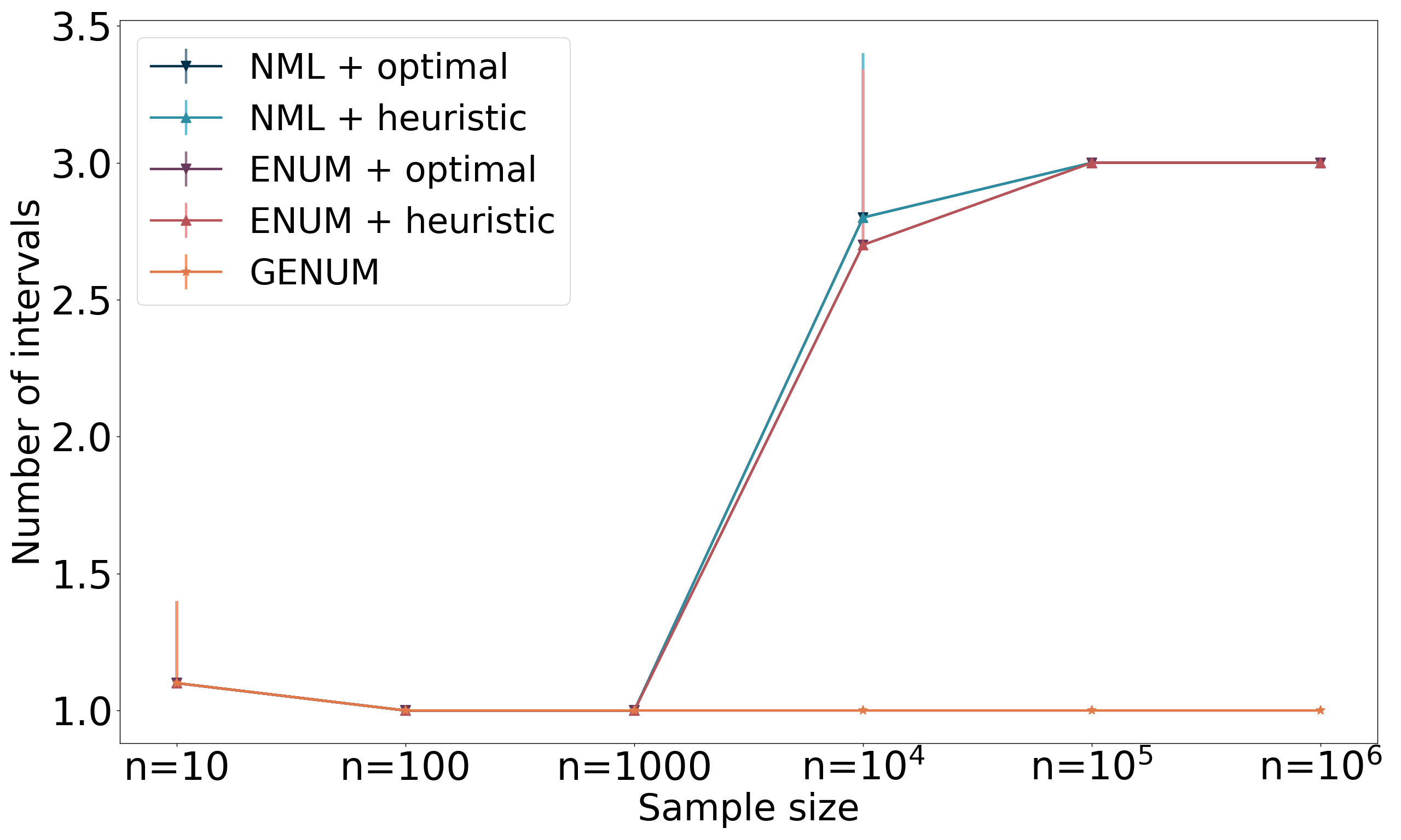
(a) Number of intervals,

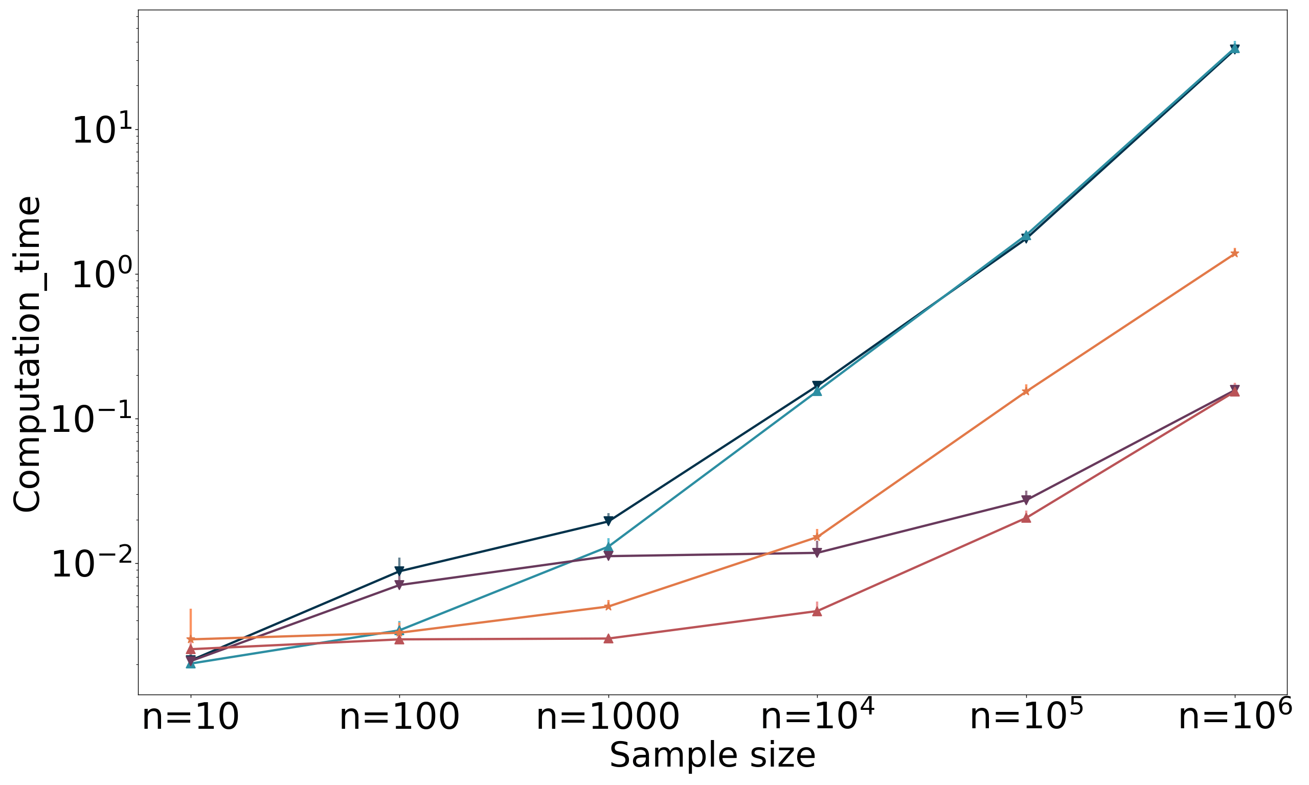
(b) Computation time,

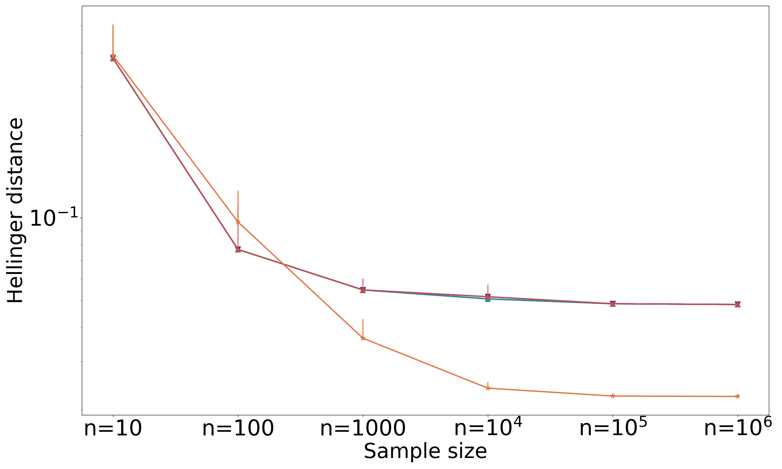
(c) Hellinger distance,

Figure 10: Comparison between MDL methods over a Triangle distribution of different sample sizes

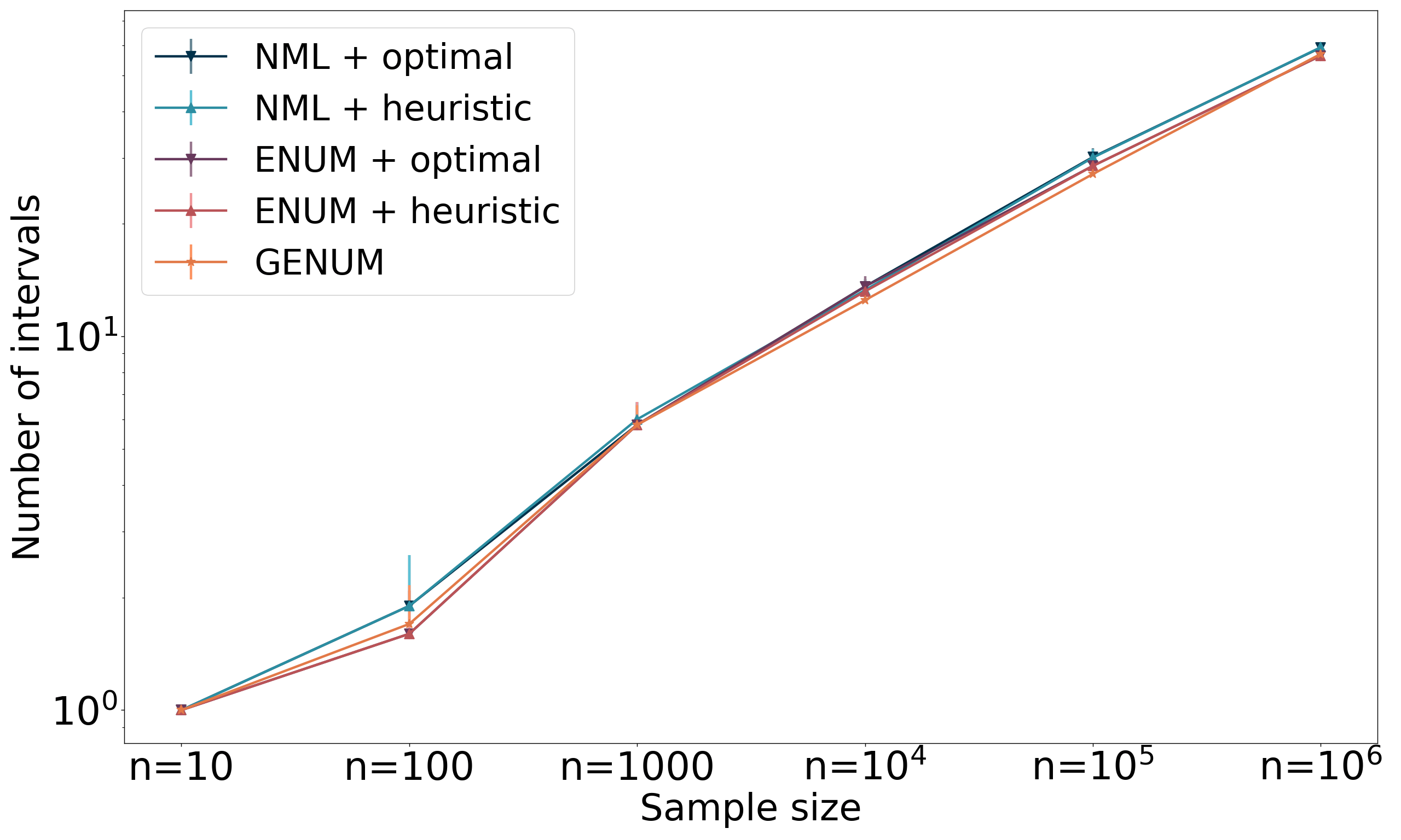
(a) Number of intervals,

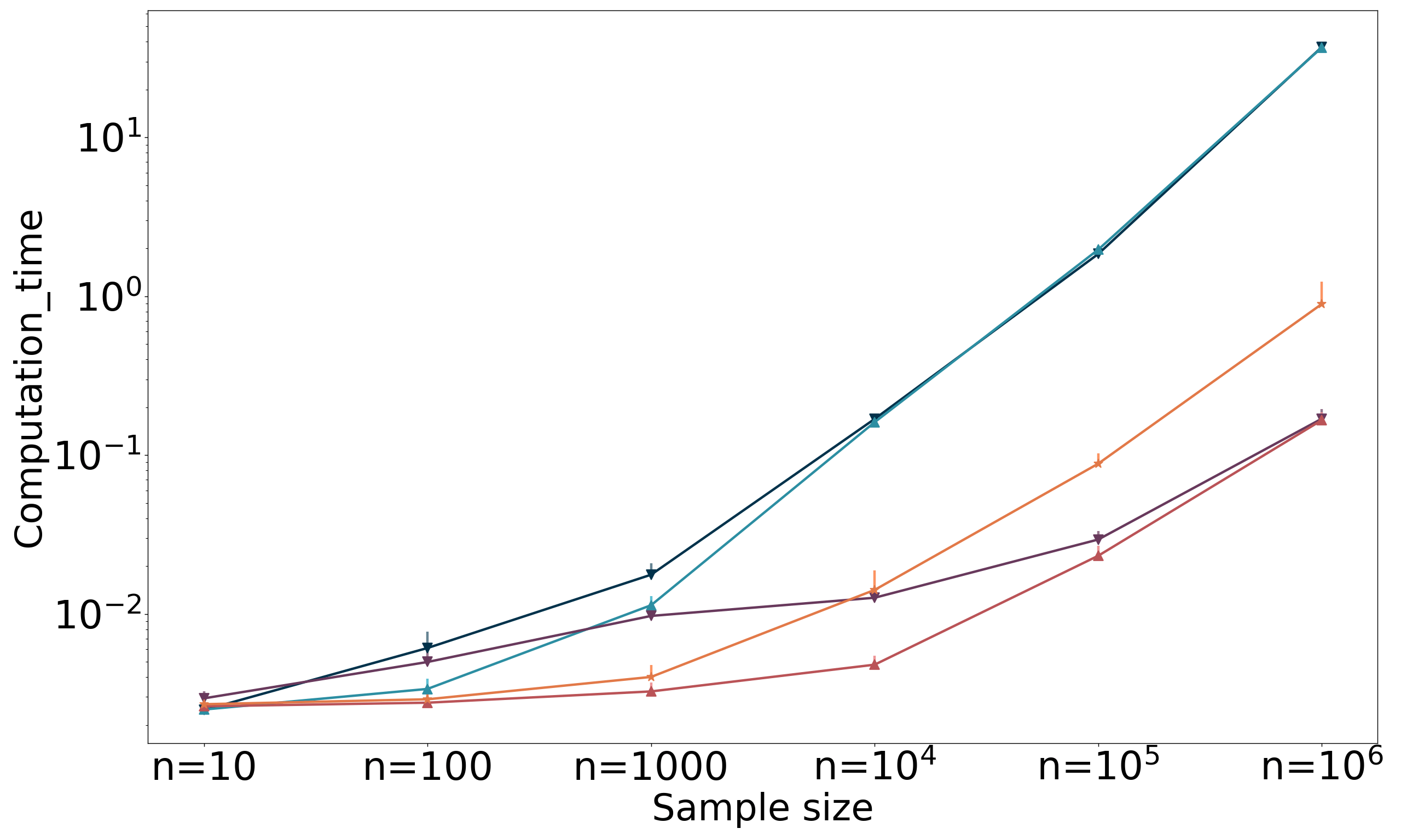
(b) Computation time,

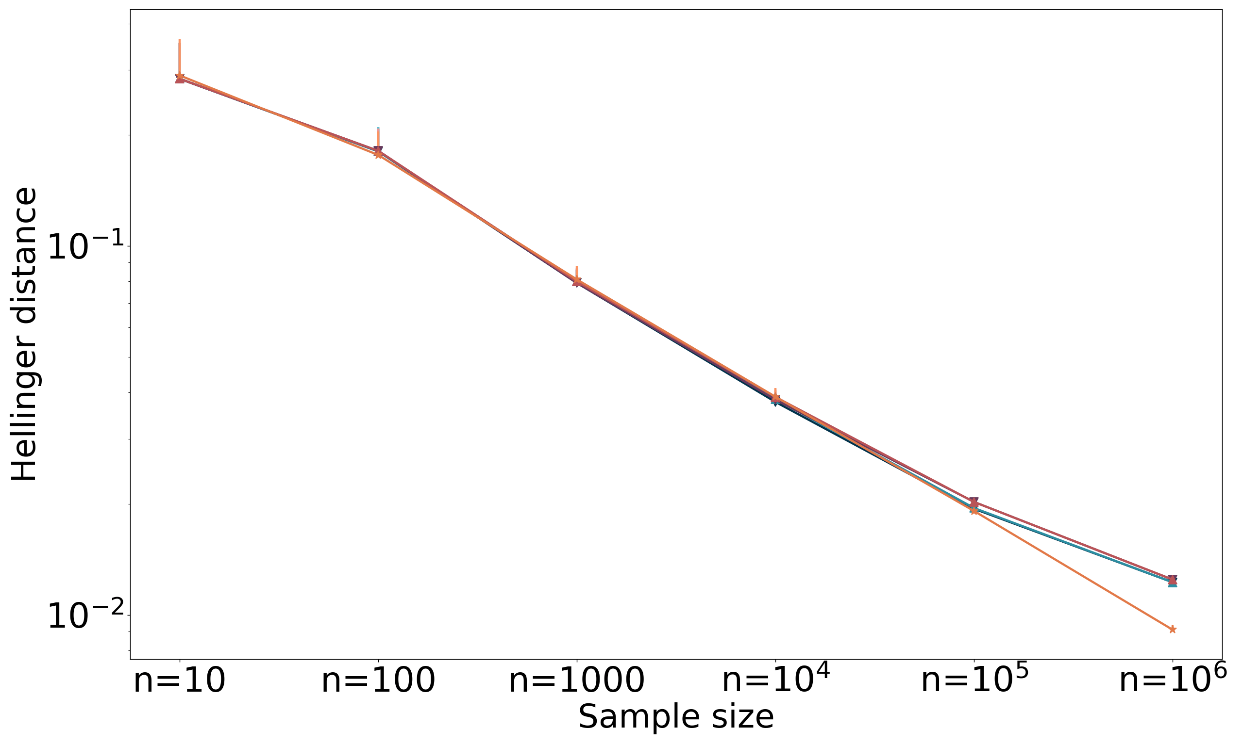
(c) Hellinger distance,

Figure 11: Comparison between MDL methods over a mixture of 4 Triangle distributions, of different sample sizes

(a) Number of intervals,

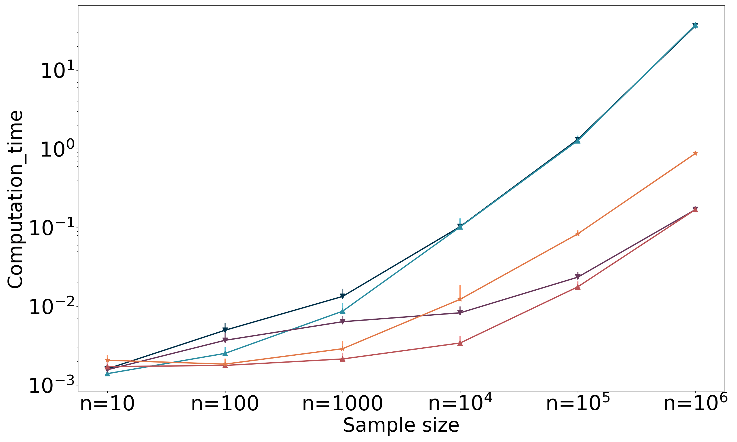
(b) Computation time,

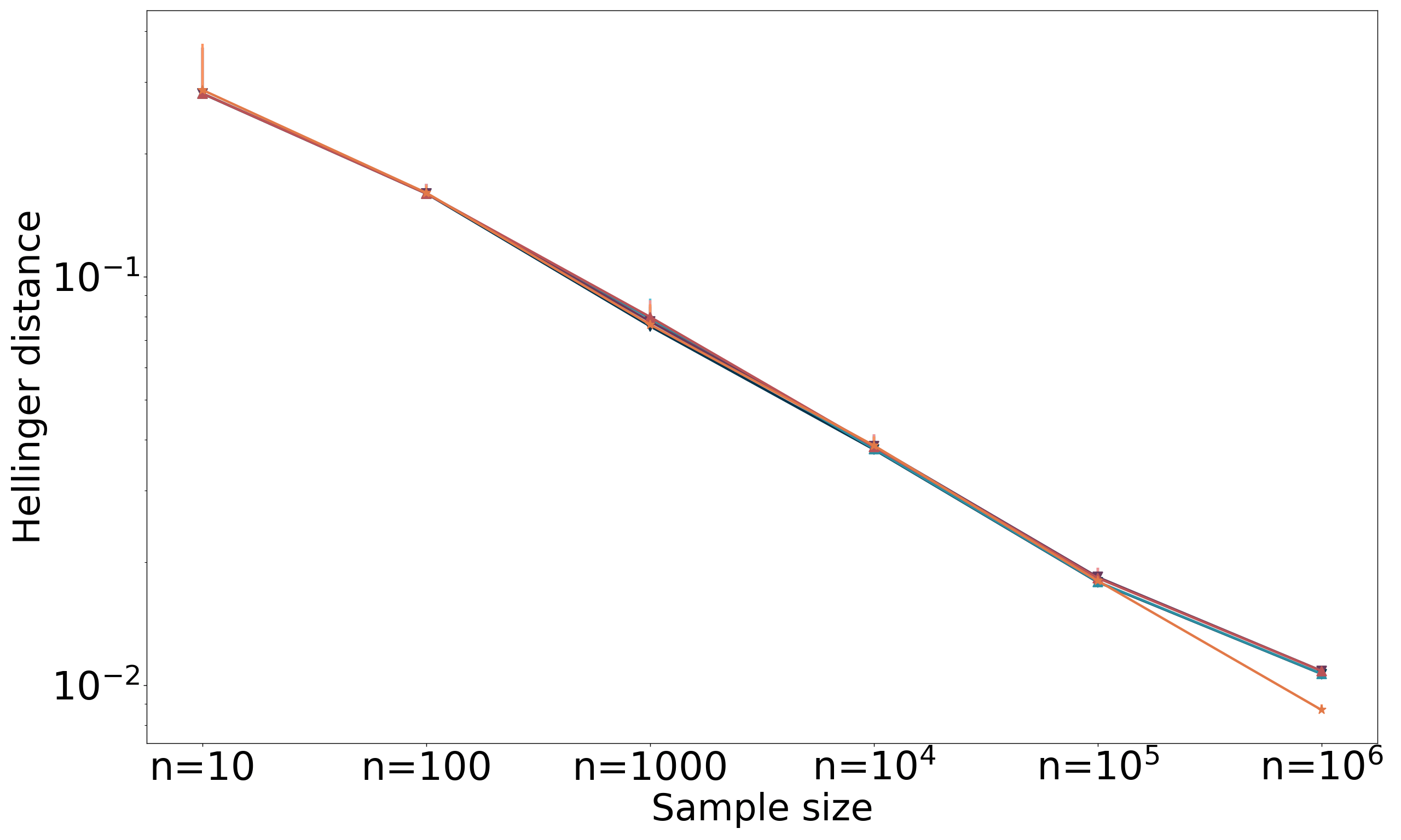
(c) Hellinger distance,

Figure 12: Comparison between MDL methods over the Claw Gaussian mixture of different sample sizes

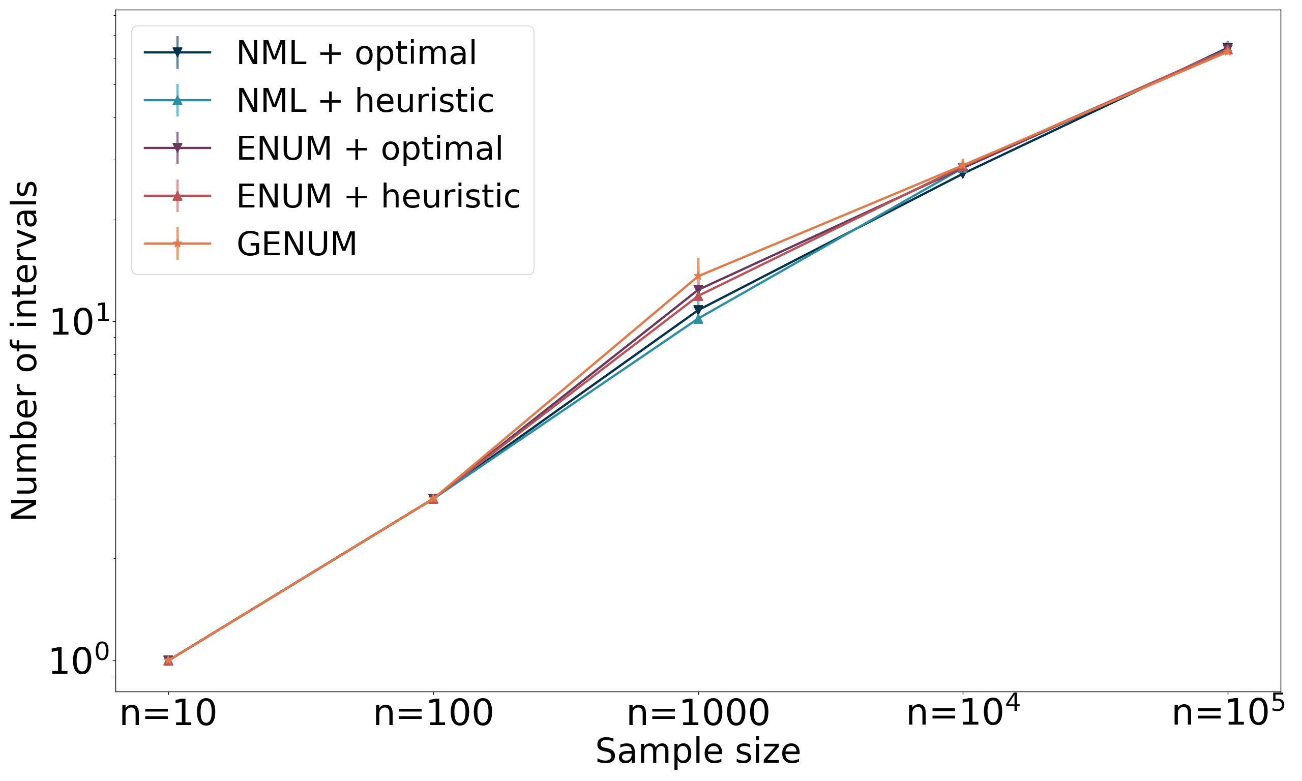
(a) Number of intervals,

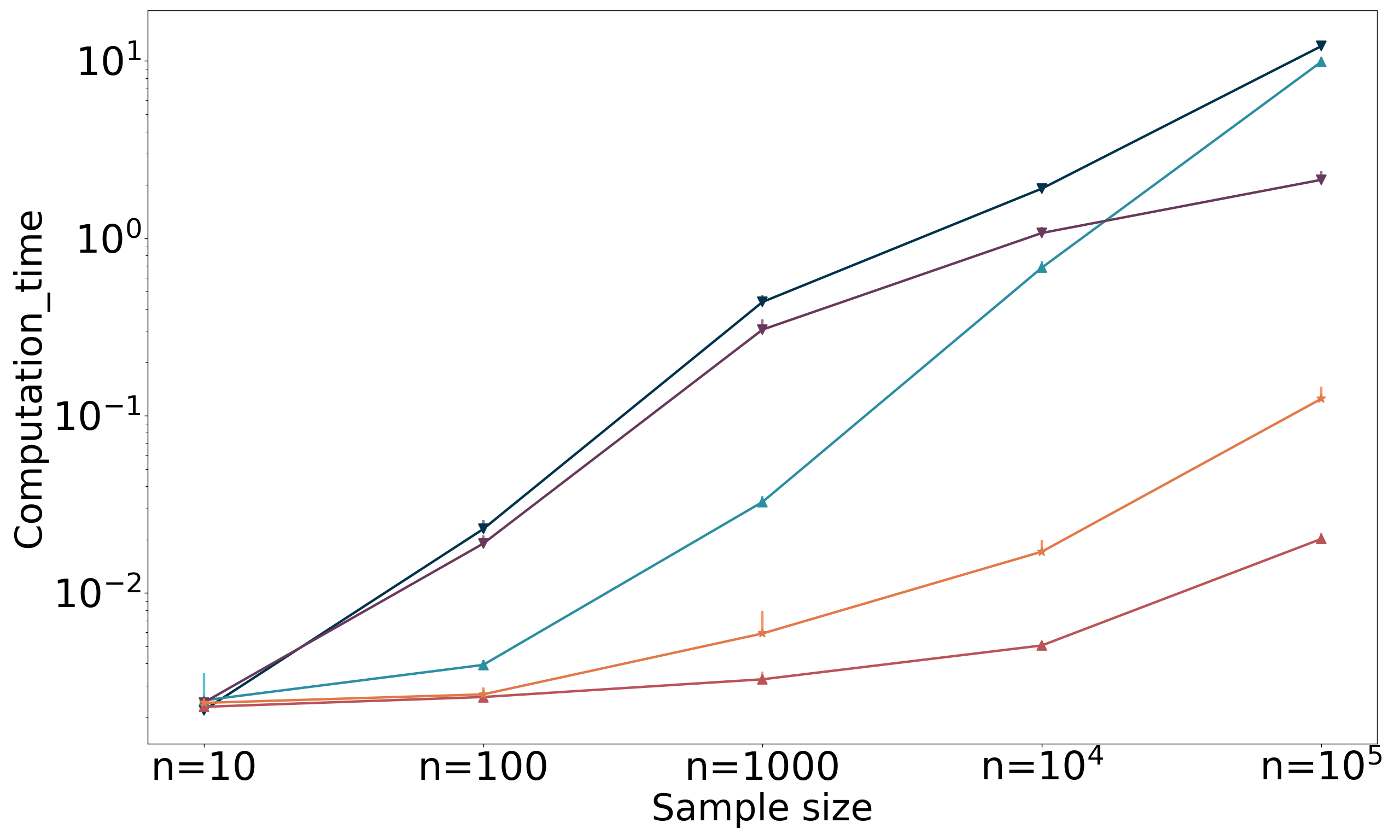
(b) Computation time,

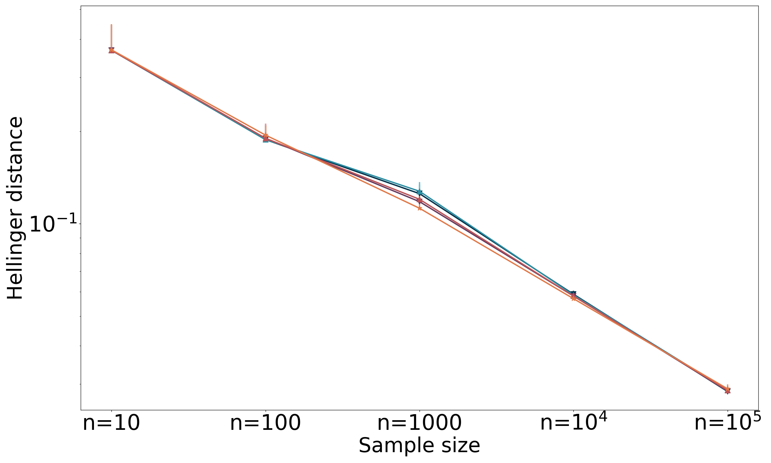
(c) Hellinger distance,

Appendix F Role of the approximation accuracy, $\epsilon$

As a complement to the theoretical analysis conducted in Section 6.2, we conducted a series of experiments to show the effect in practice of using a too small value for $\epsilon$. We compare all MDL methods over a Normal distribution of small size ($n=100$ and $n=1000$), for $\epsilon$ ranging from $2.0$ to $10^{-8}$.

Figures 13 and 14 summarise the results. For both sample sizes we can observe that, as $\epsilon\rightarrow 0$, the number of intervals in NML and Enum histograms decreases. Particularly, for the $n=100$ distribution, the estimations models start at 3 intervals and NML and Enum histograms slowly decrease to having a single one. This observation is in line with Corollary 1.

In stark contrast, G-Enum remains at 3 intervals throughout. The same consistency can be observed in regards to computation times and Hellinger distance. While the NML and Enum methods take more time and produce lower quality results as the approximation accuracy increases, the G-Enum steadily produces quality results in less time.

Note also that the best value for $\epsilon$ is different for both sample sizes. For a distribution of $n=100$ samples, having $\epsilon=0.1$ guarantees the lowest Hellinger distance for the NML and Enum methods. For $n=1000$ samples, it is preferable to set $\epsilon=0.5$. When we do not know anything about the nature of the data, there is no guarantee we will make the right choice for NML and Enum. On the other hand, our granularised approach automatically selects $\epsilon^{*}\approx 1.324$ and $\epsilon^{*}\approx 0.178$ for samples sizes $n=100$ and $n=1000$ respectively. While these choices certainly do not achieve the lowest HD technically possible, they have the merit of not being too far off. G-Enum histograms seem to select fair enough accuracy values for a fully automated estimation.

These sensitivity experiments have shown that the value of $\epsilon$ cannot be overlooked as easily as thought: for some distributions and middle-range sample sizes, the approximation accuracy can play an important role in computation time and estimation quality. In an exploratory analysis context, where little is known about the data, a truly fully automated approach such as G-Enum is preferable than the other MDL methods.

Figure 13: Comparison of MDL methods over a Normal distribution of size $n=100$ for different values of $\epsilon$

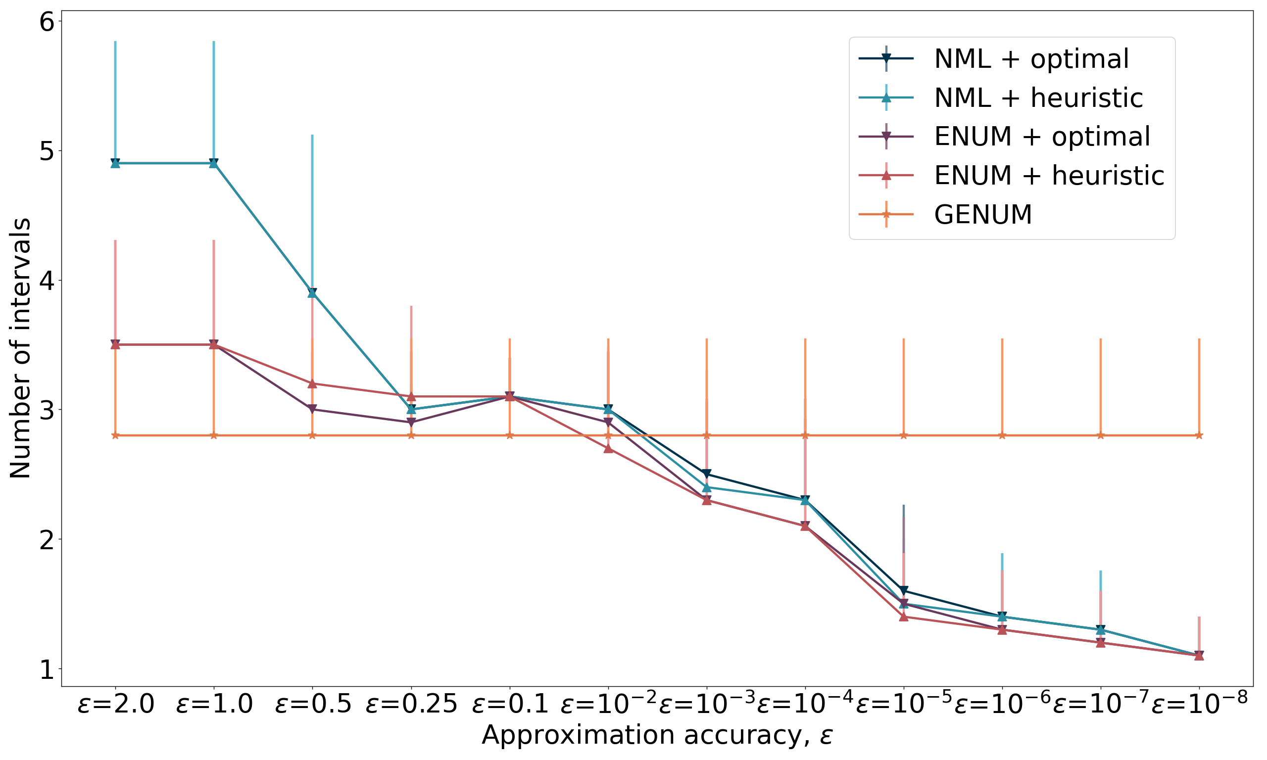
(a) Number of intervals,

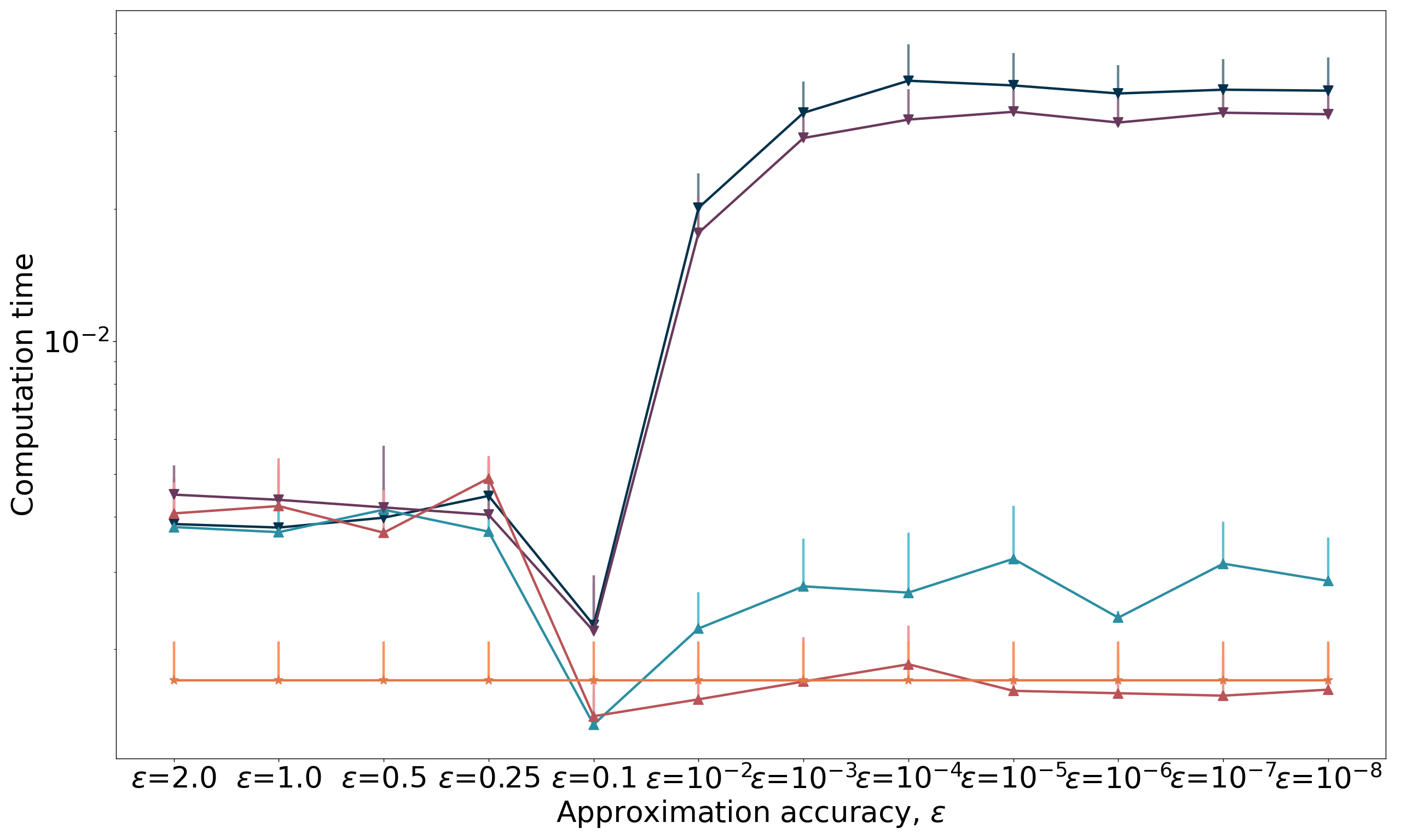
(b) Computation time,

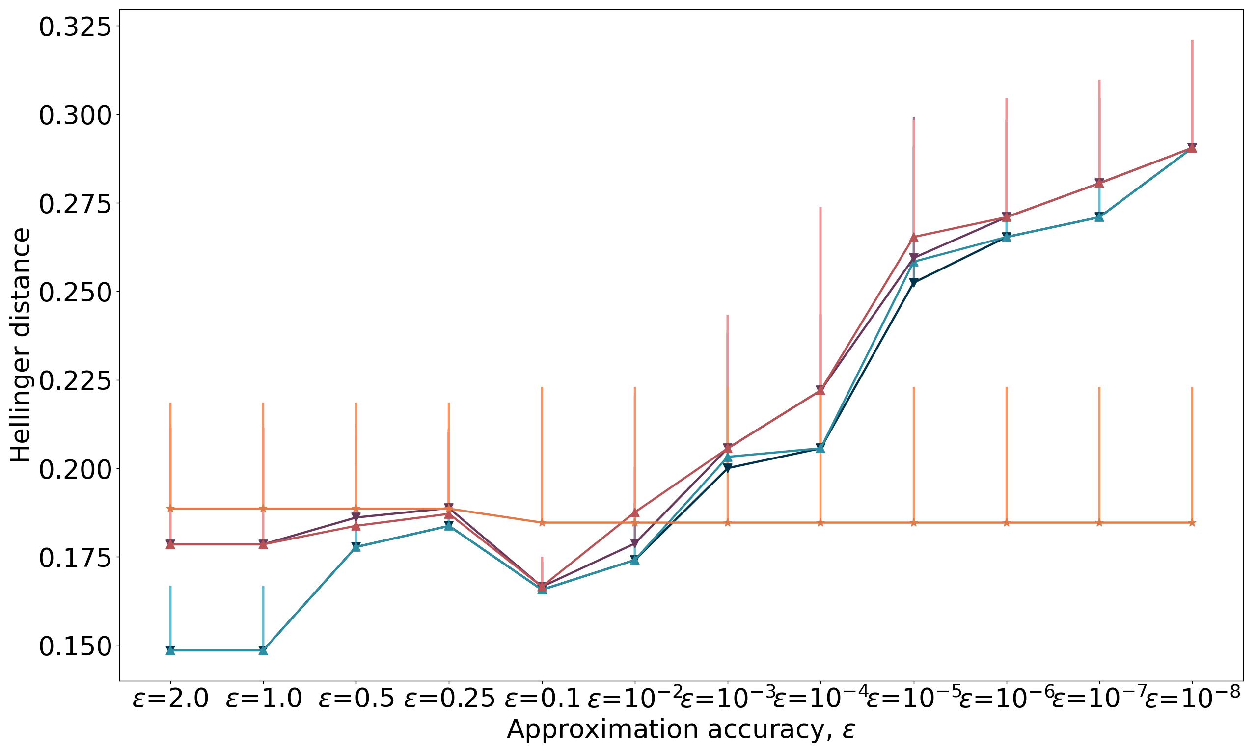
(c) Hellinger distance,

Figure 14: Comparison of MDL methods over a Normal distribution of size $n=1000$ for different values of $\epsilon$

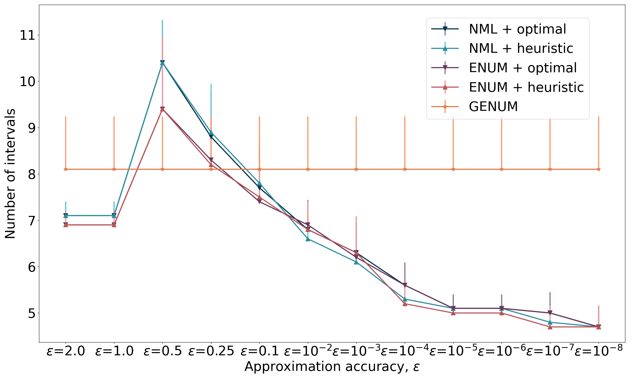
(a) Number of intervals,

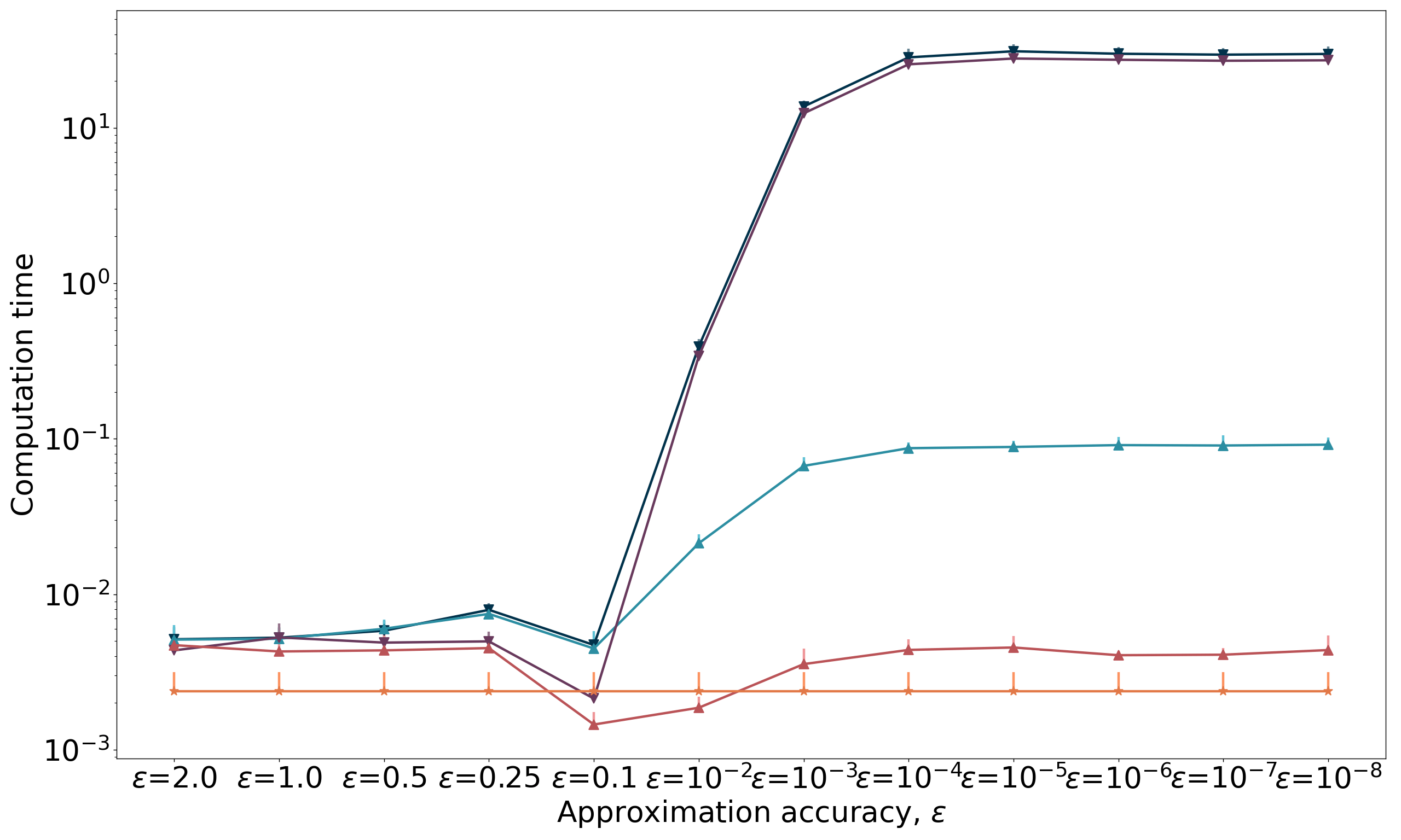
(b) Computation time,

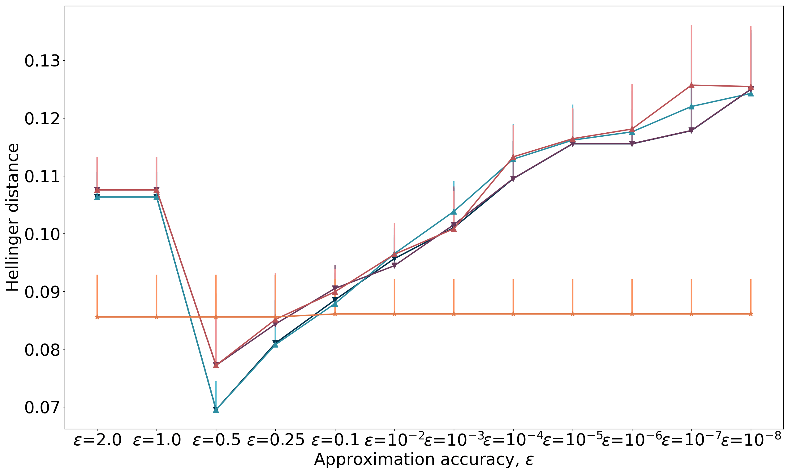
(c) Hellinger distance,

Appendix G Benchmarking and comparison with other methods

The last series of figures compare the NML and G-Enum criteria to other 5 state-of-the-art methods for building histograms.

All 7 methods are evaluated on different sample sizes of a Normal (figures 15 and 16, Cauchy (figures 17 and 18), uniform (figures 19 and 20), triangle (figures 21 and 22), triangle mixture (figures 23 and 24) and Gaussian mixture (figures 25 and 26) distributions.

We highlight that all results are means over 10 experiments for each sample size. All results are shown in log scale. The standard deviations of the metrics are represented asymmetrically in the graphs to because of the log scale.

Figure 15: Different histograms obtained for a single Normal distribution of size $n=10^{4}$

(a) A Normal distribution

(b) NML + heuristic ($K^{*}=16$)

(c) G-Enum ($K^{*}=17$)

(d) Bayesian blocks ($K^{*}=16$)

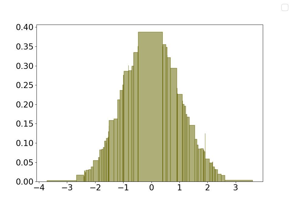
(e) Taut string ($K^{*}=68$)

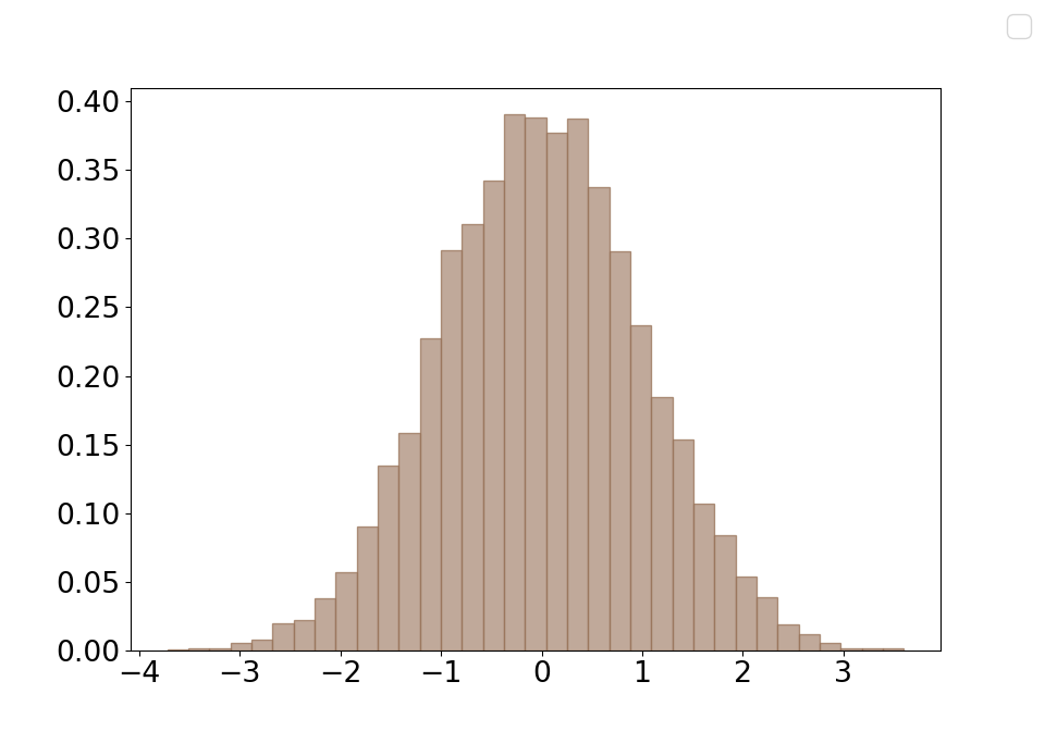
(f) RMG ($K^{*}=35$)

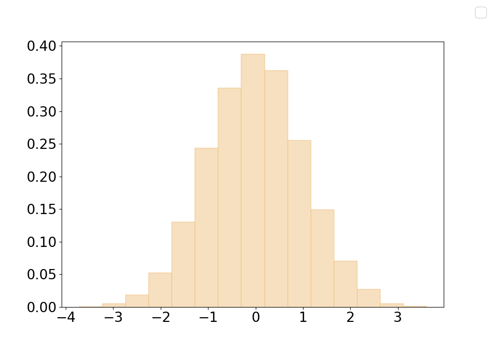
(g) Sturges ($K^{*}=15$)

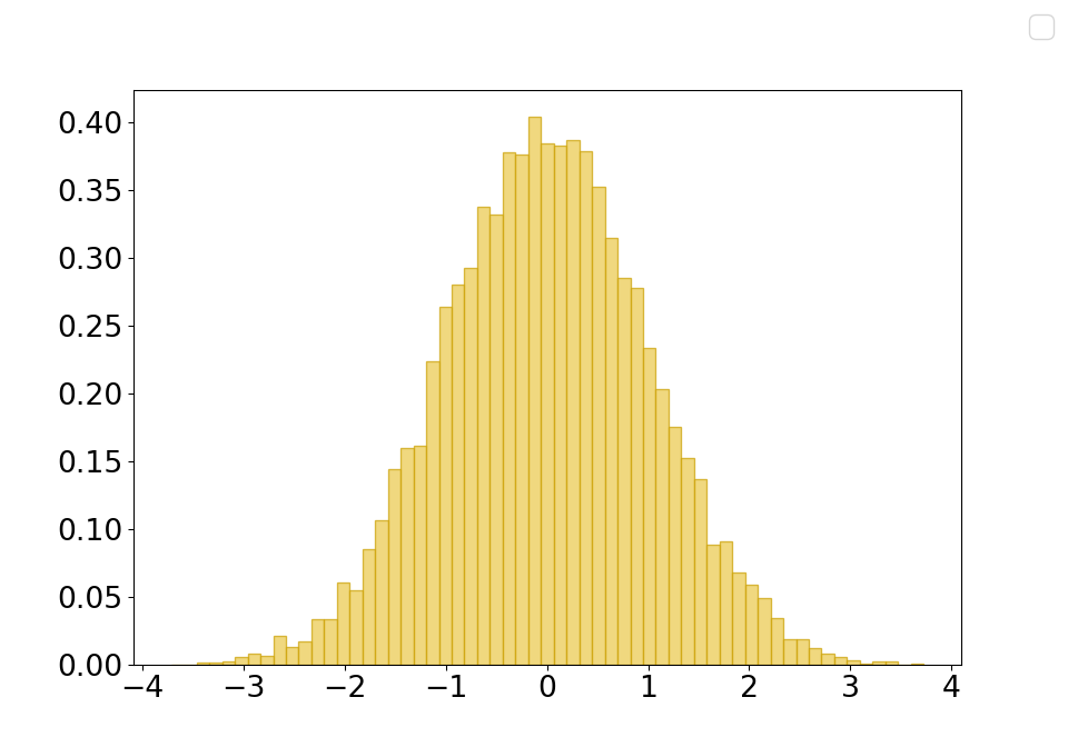
(h) Freedman-Diaconis ($K^{*}=59$)

Figure 16: Comparison with state-of-the-art methods over a Normal distribution of different sample sizes

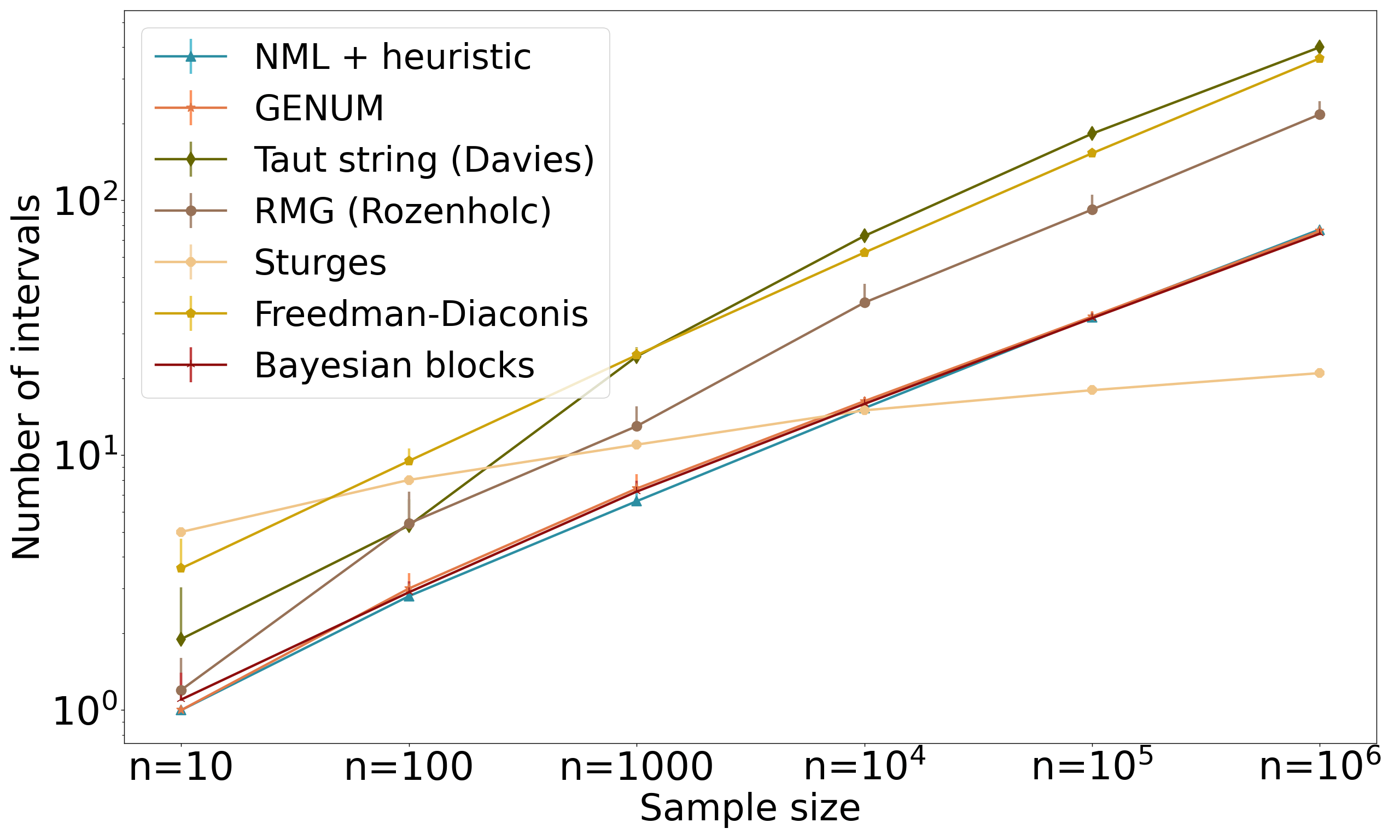
(a) Number of intervals,

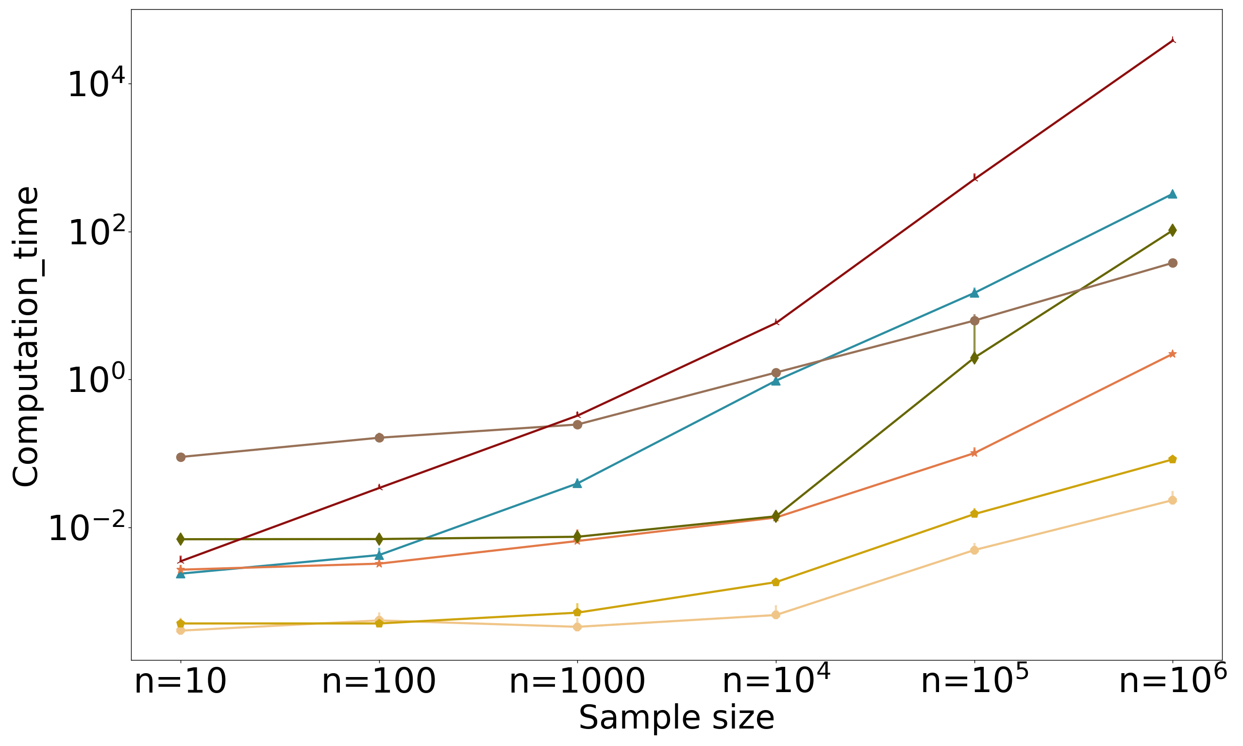
(b) Computation time,

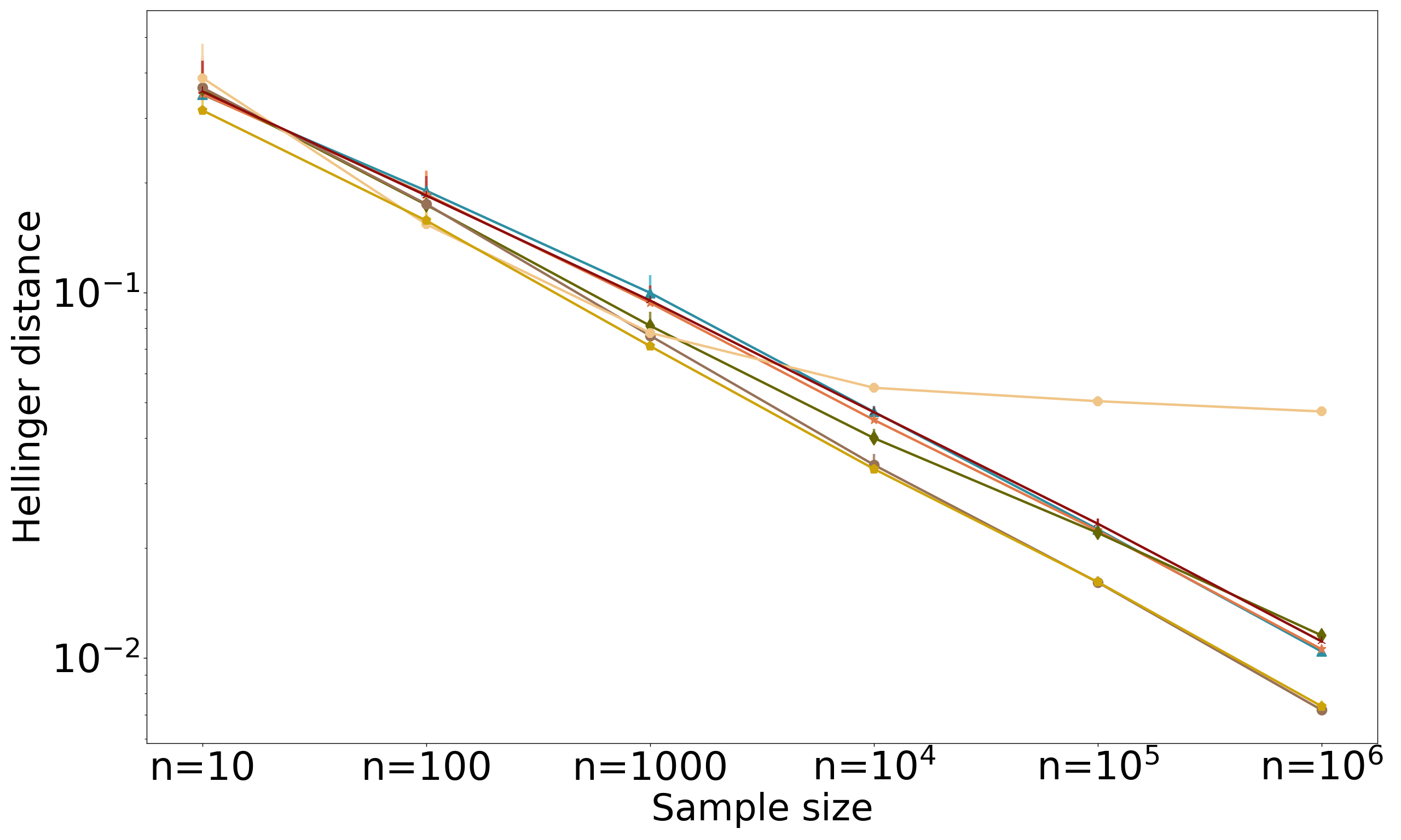
(c) Hellinger distance,

Figure 17: Different histograms obtained for a single Cauchy distribution of size $n=10^{4}$

(a) A Cauchy distribution in $\log$ scale

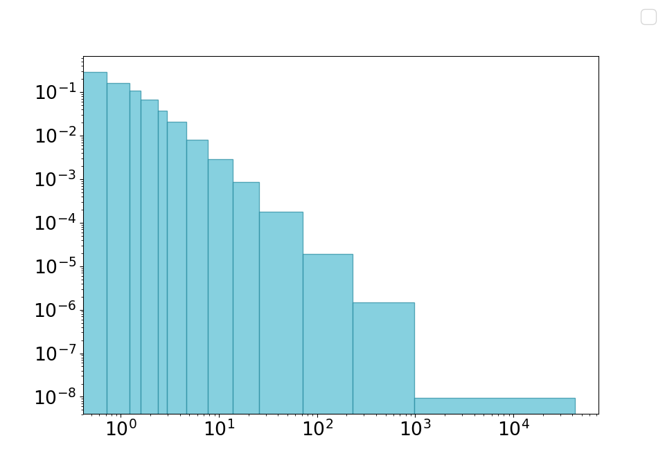
(b) NML + heuristic ($K^{*}=24$)

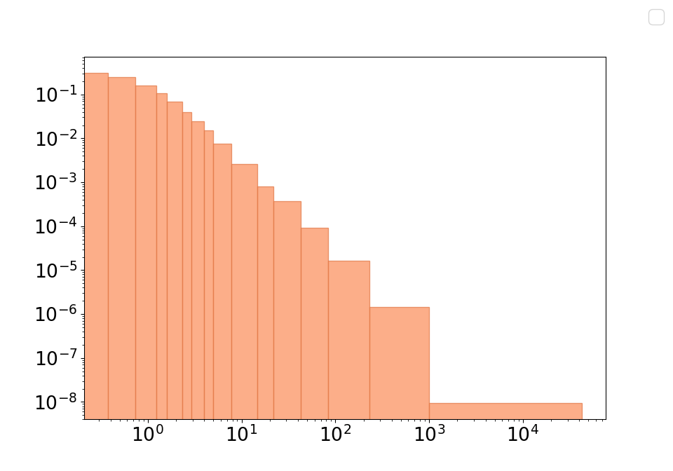
(c) G-Enum ($K^{*}=30$)

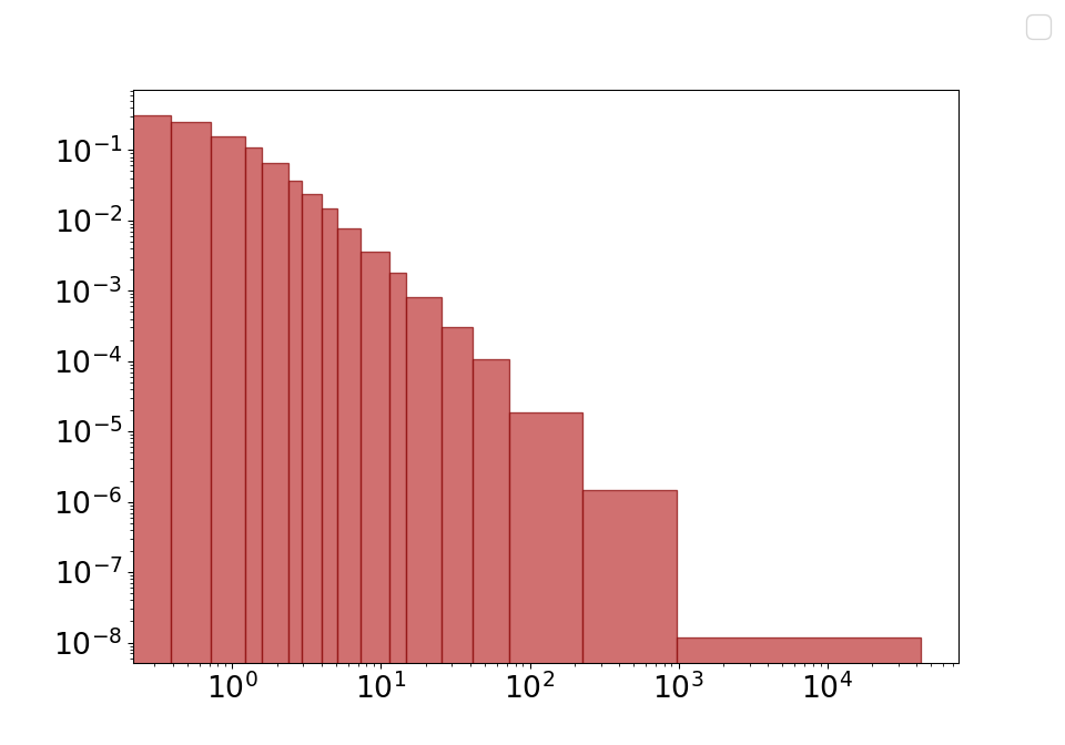
(d) Bayesian blocks ($K^{*}=32$)

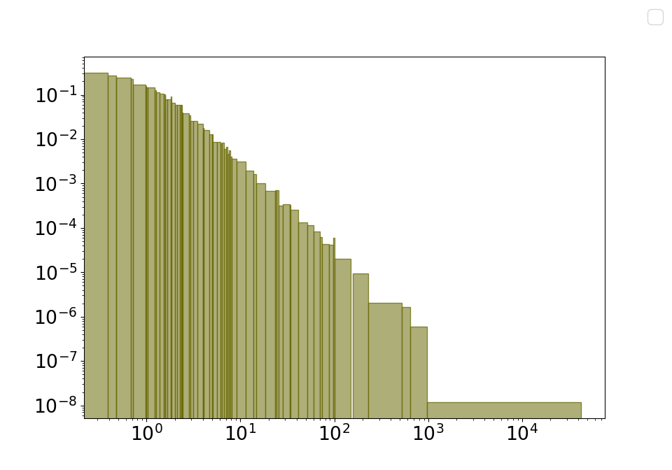
(e) Taut string ($K^{*}=141$)

(f) RMG ($K^{*}=31$)

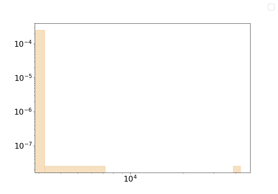
(g) Sturges ($K^{*}=15$)

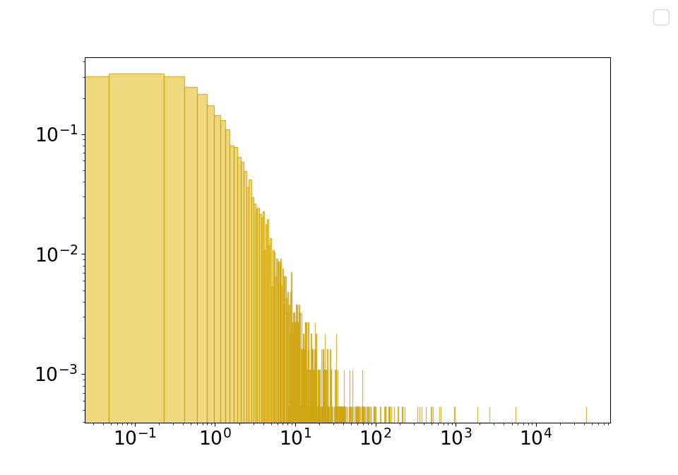
(h) Freedman-Diaconis ($K^{*}=319399$)

Figure 18: Comparison with state-of-the-art methods over a Cauchy distribution of different sample size

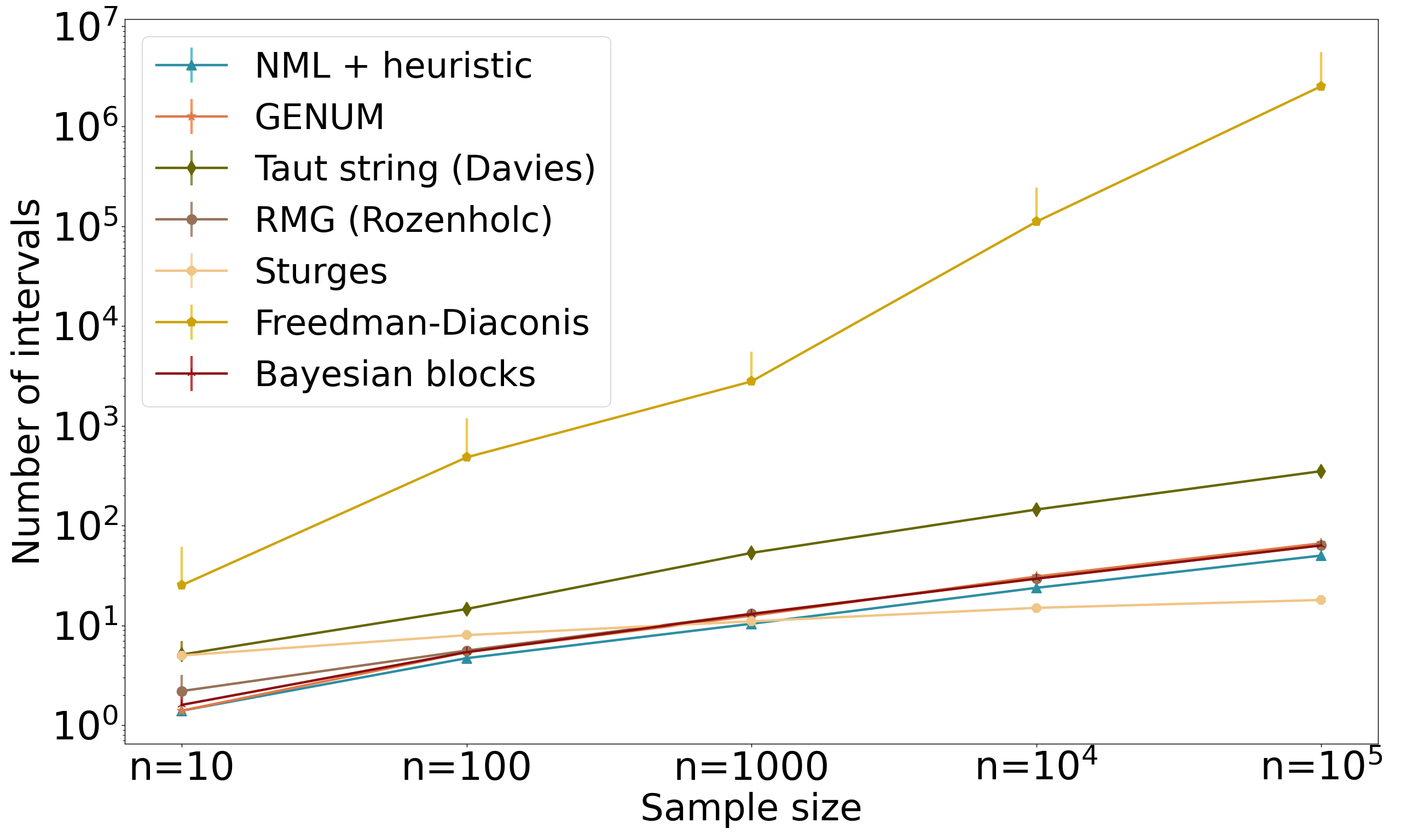
(a) Number of intervals,

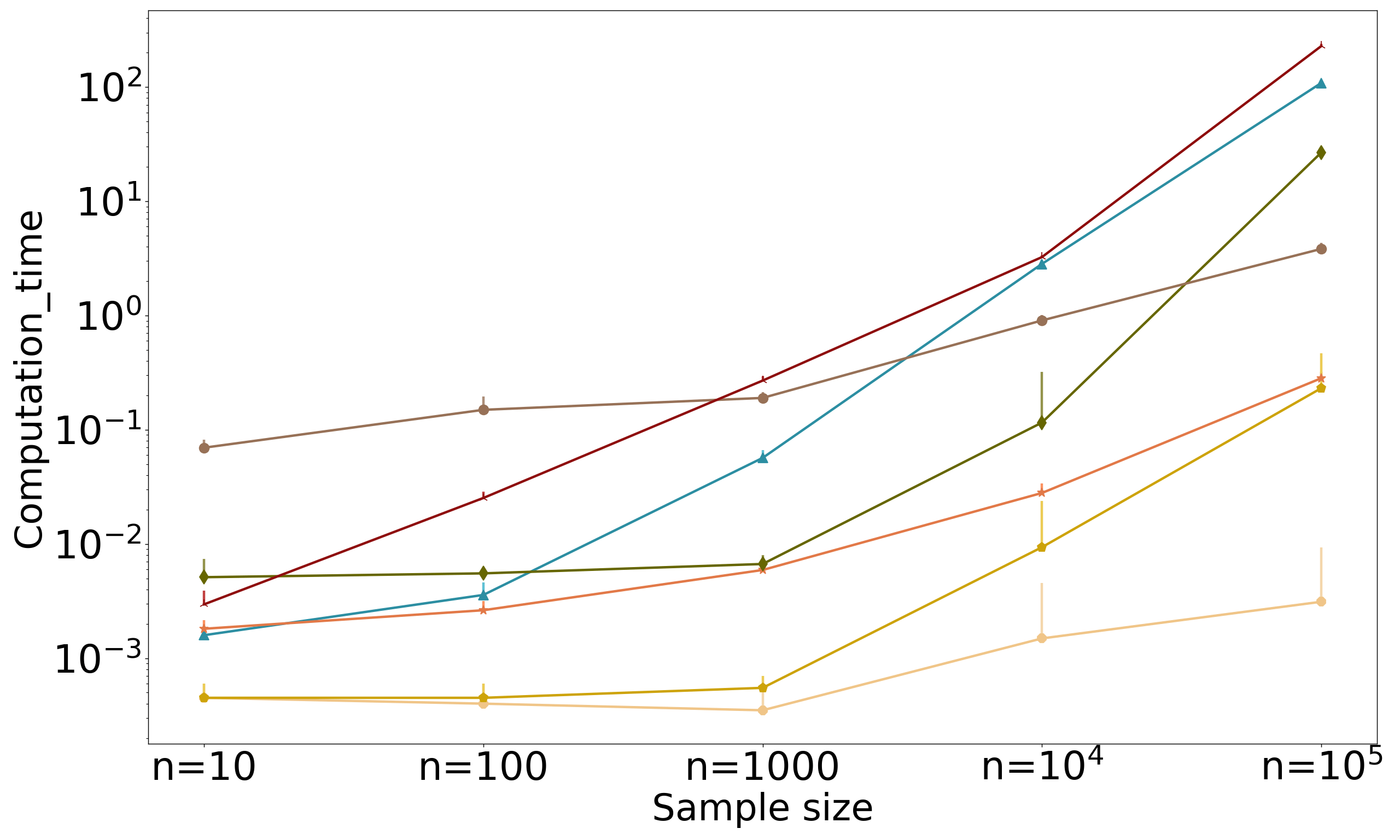
(b) Computation time,

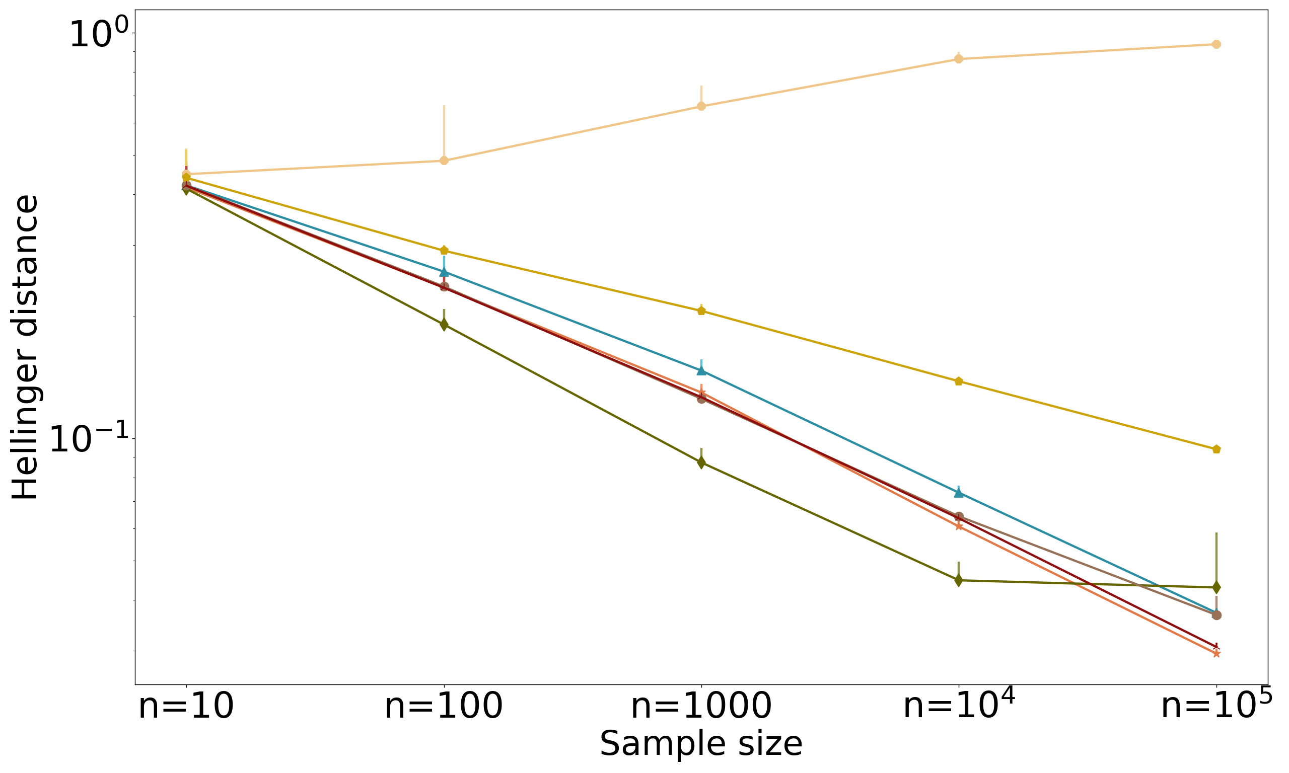
(c) Hellinger distance,

Figure 19: Different histograms obtained for a single uniform distribution of size $n=10^{4}$

(a) A uniform distribution

(b) NML + heuristic ($K^{*}=3$)

(c) G-Enum ($K^{*}=1$)

(d) Bayesian blocks ($K^{*}=1$)

(e) Taut string ($K^{*}=1$)

(f) RMG ($K^{*}=1$)

(g) Sturges ($K^{*}=15$)

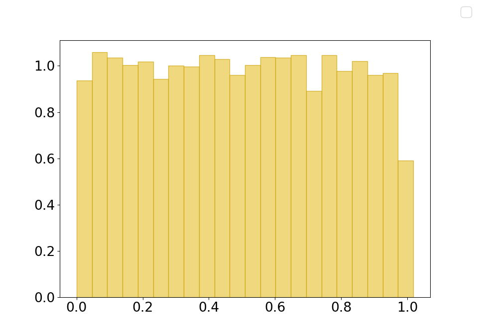
(h) Freedman-Diaconis ($K^{*}=22$)

Figure 20: Comparison with other methods over a uniform distribution of different sample size

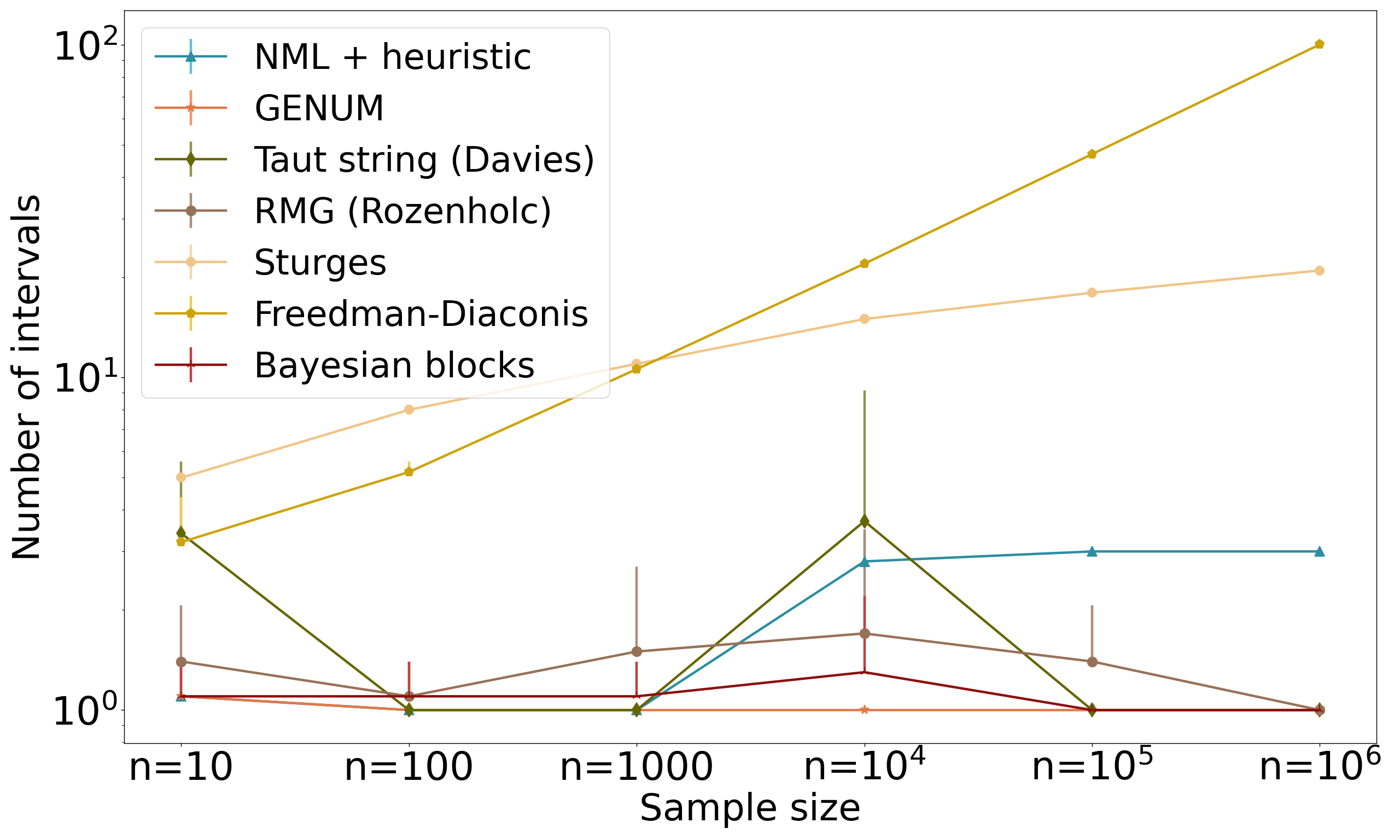
(a) Number of intervals,

(b) Computation time,

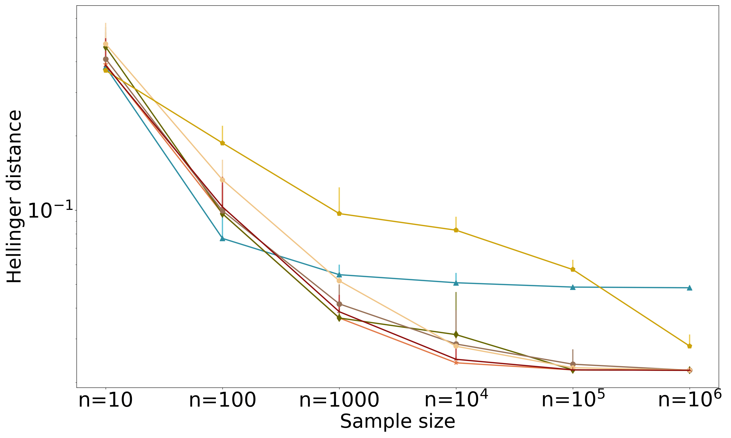
(c) Hellinger distance,

Figure 21: Different histograms obtained for a single Triangle distribution of size $n=10^{4}$

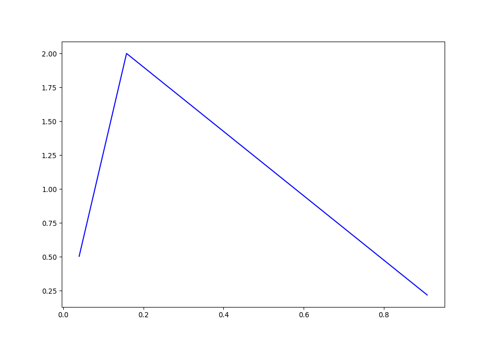
(a) A triangle distribution

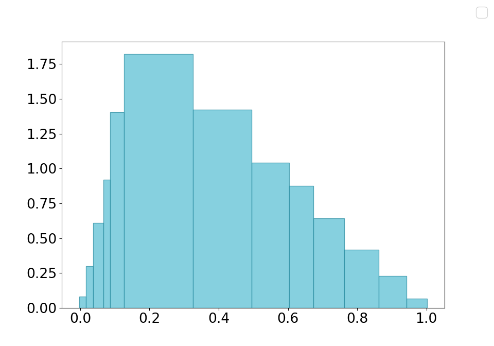
(b) NML + heuristic ($K^{*}=13$)

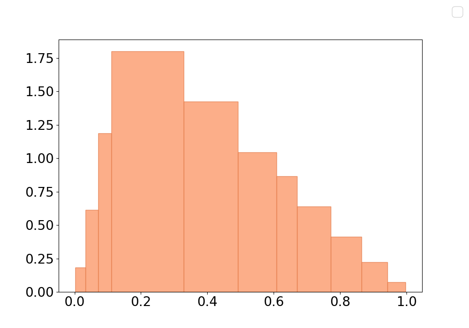
(c) G-Enum ($K^{*}=11$)

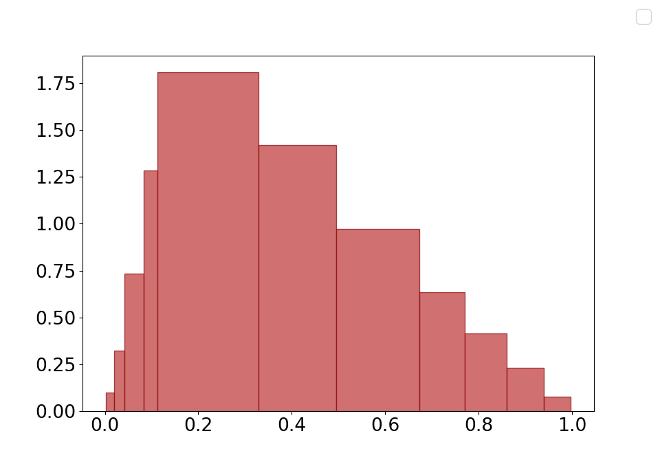
(d) Bayesian blocks ($K^{*}=11$)

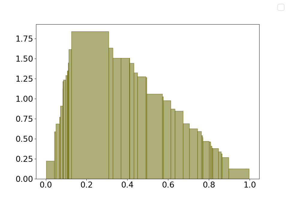
(e) Taut string ($K^{*}=43$)

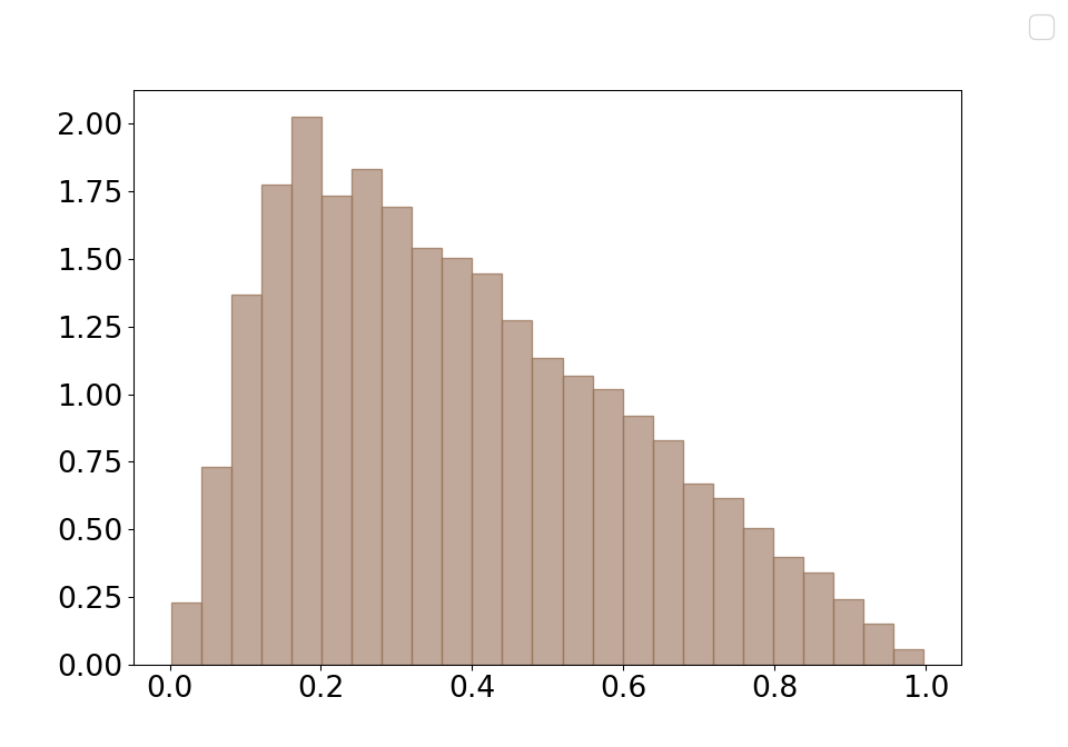
(f) RMG ($K^{*}=25$)

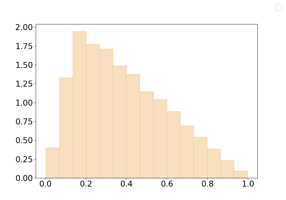
(g) Sturges ($K^{*}=15$)

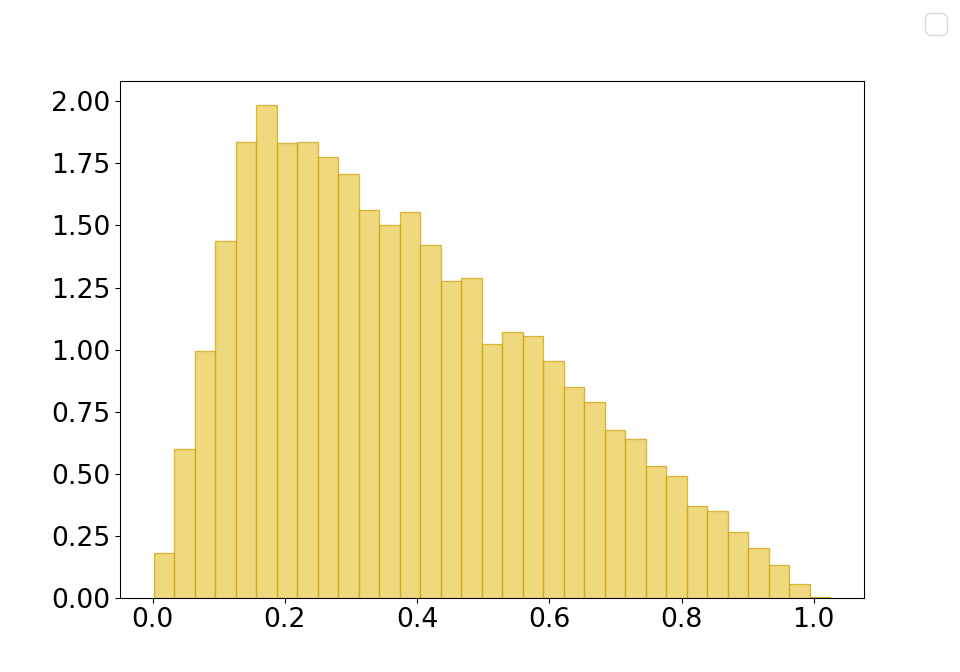
(h) Freedman-Diaconis ($K^{*}=33$)

Figure 22: Comparison with state-of-the-art methods over a Triangle distribution of different sample sizes

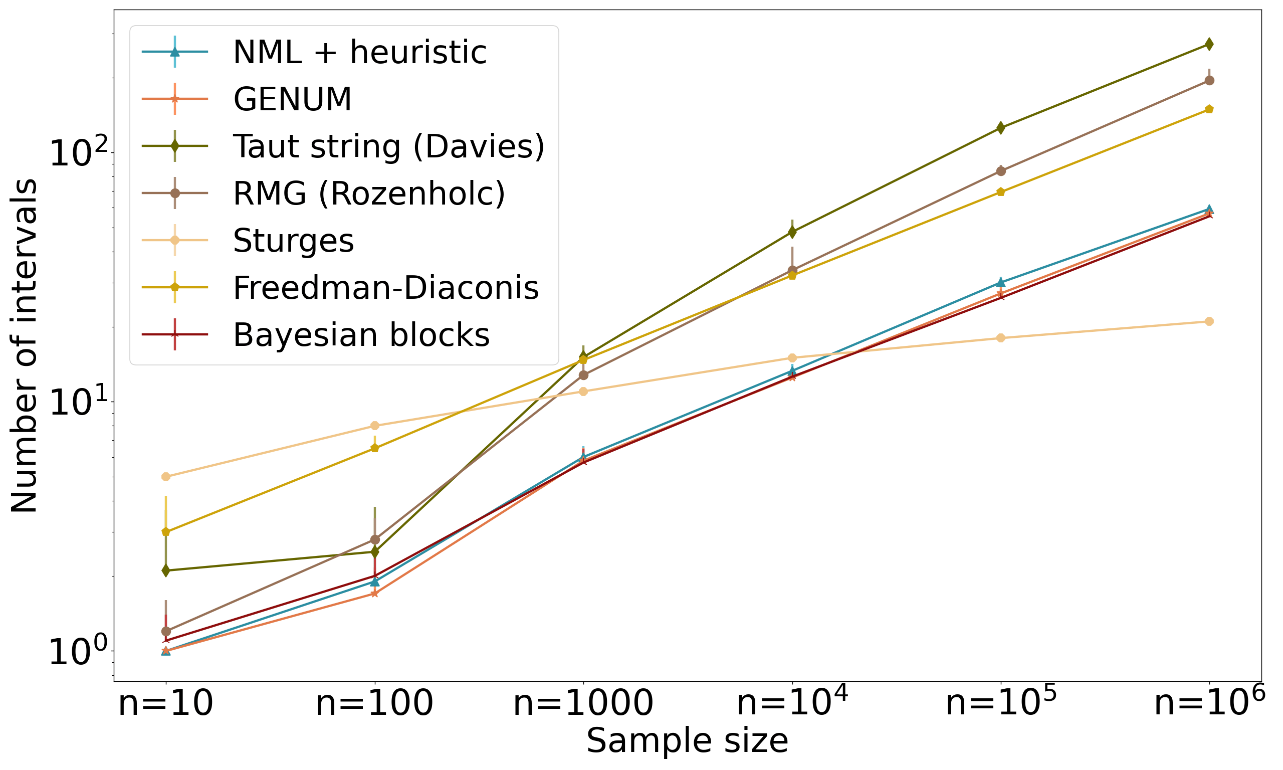
(a) Number of intervals,

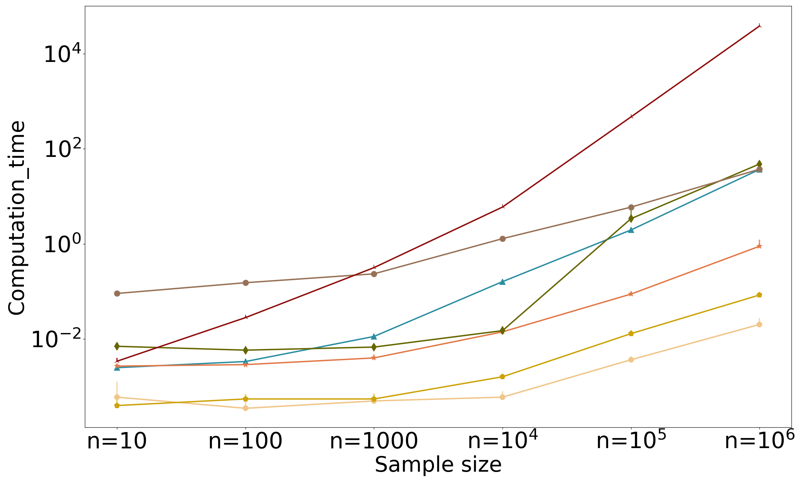
(b) Computation time,

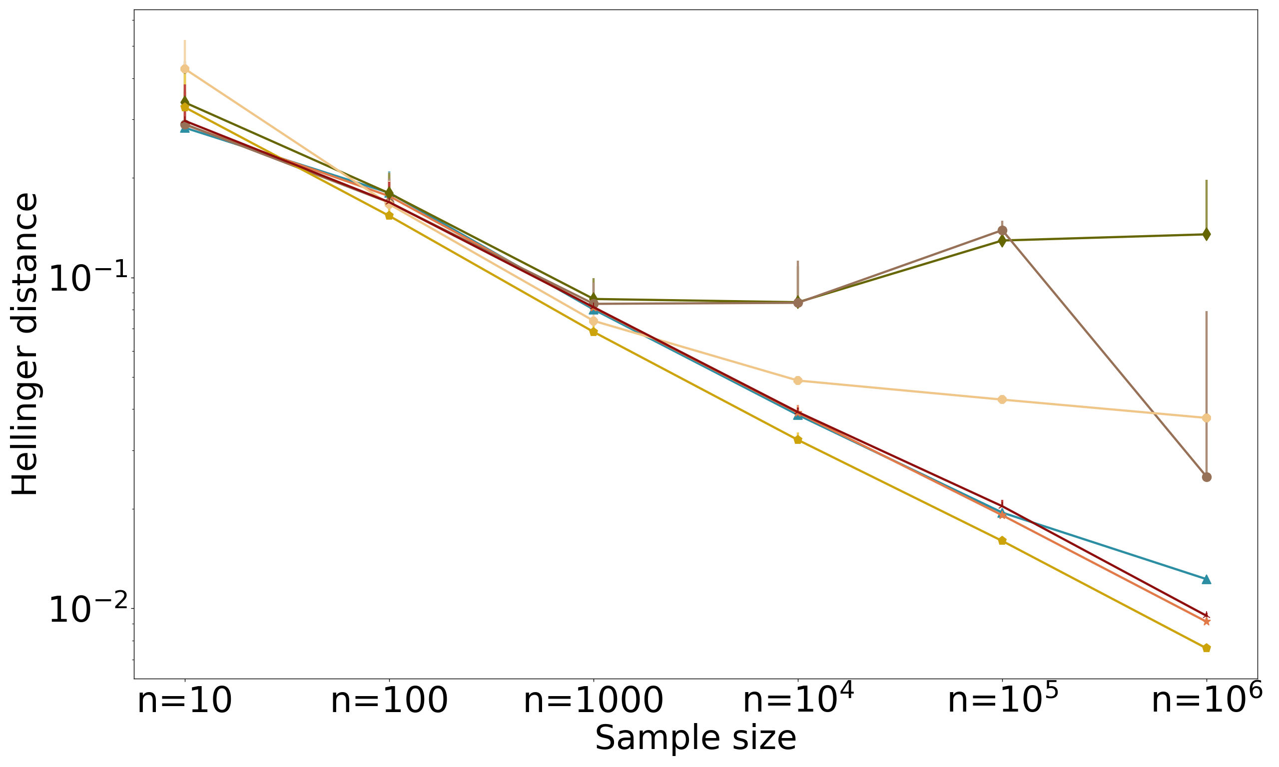
(c) Hellinger distance,

Figure 23: Different histograms obtained for a single mixture of 4 triangle distributions, of size $n=10^{4}$

(a) A triangle mixture

(b) NML + heuristic ($K^{*}=12$)

(c) G-Enum ($K^{*}=12$)

(d) Bayesian blocks ($K^{*}=11$)

(e) Taut string ($K^{*}=53$)

(f) RMG ($K^{*}=38$)

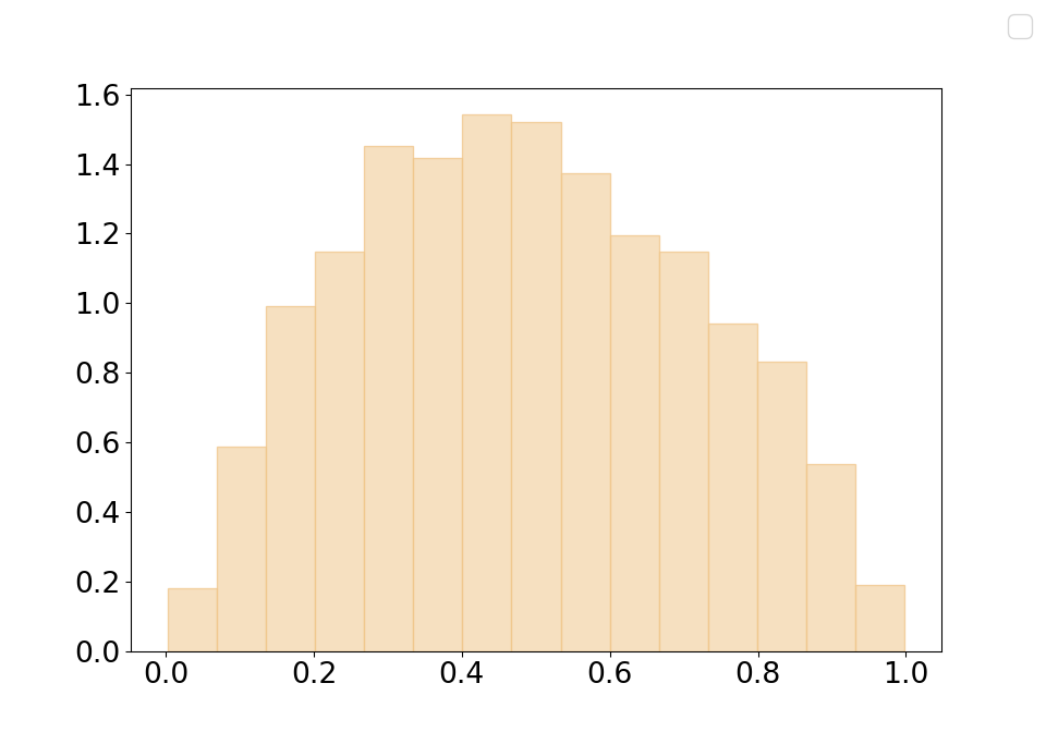
(g) Sturges ($K^{*}=15$)

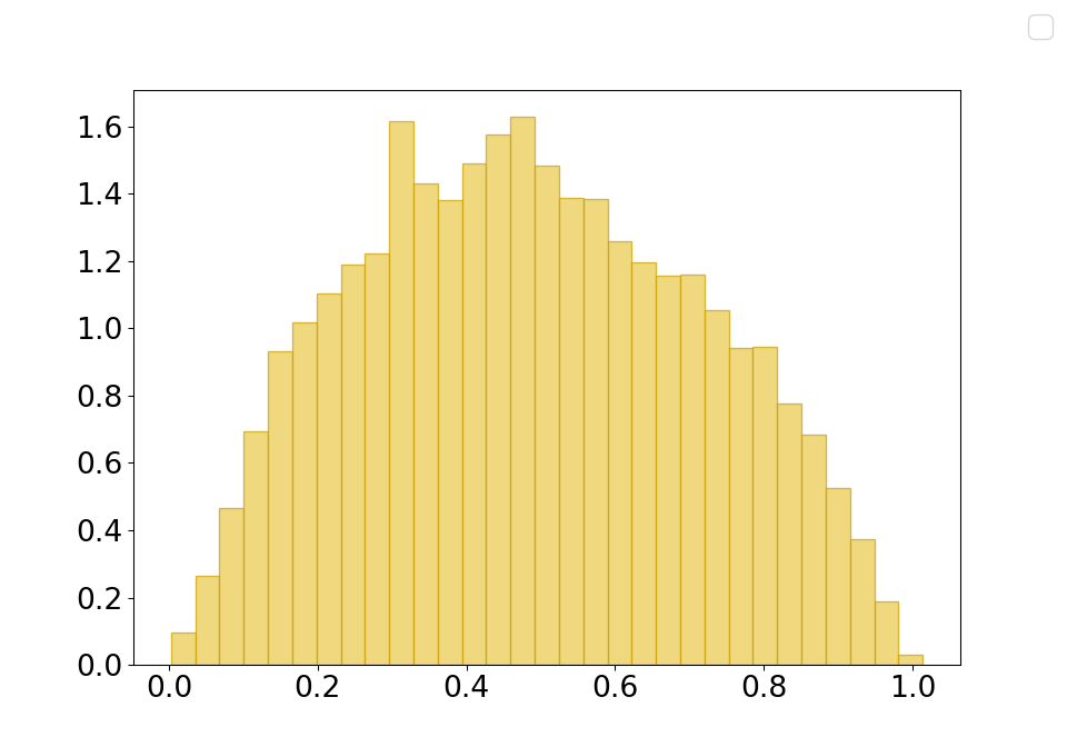
(h) Freedman-Diaconis ($K^{*}=31$)

Figure 24: Comparison with state-of-the-art methods over a mixture of 4 Triangle distributions, of different sample sizes

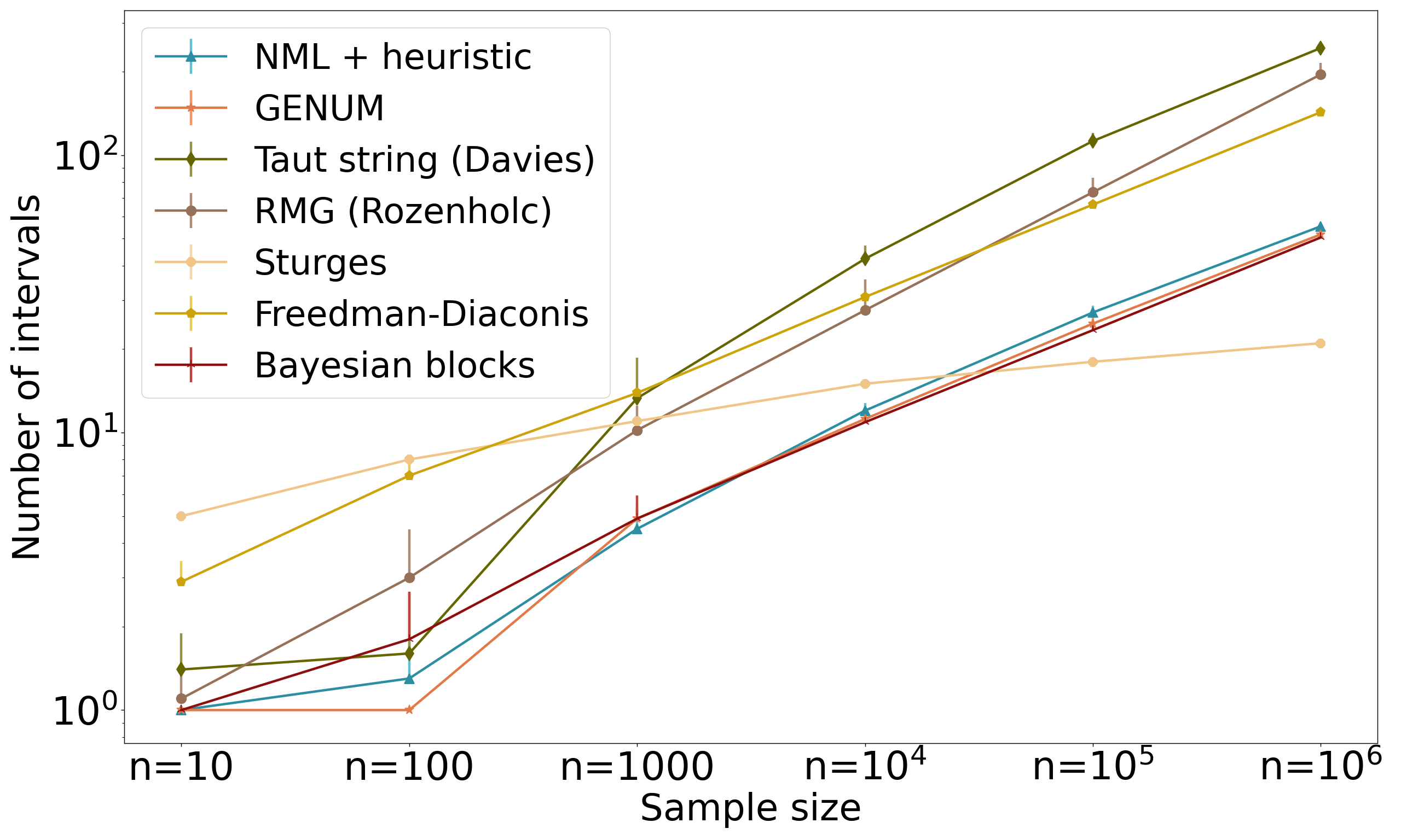
(a) Number of intervals,

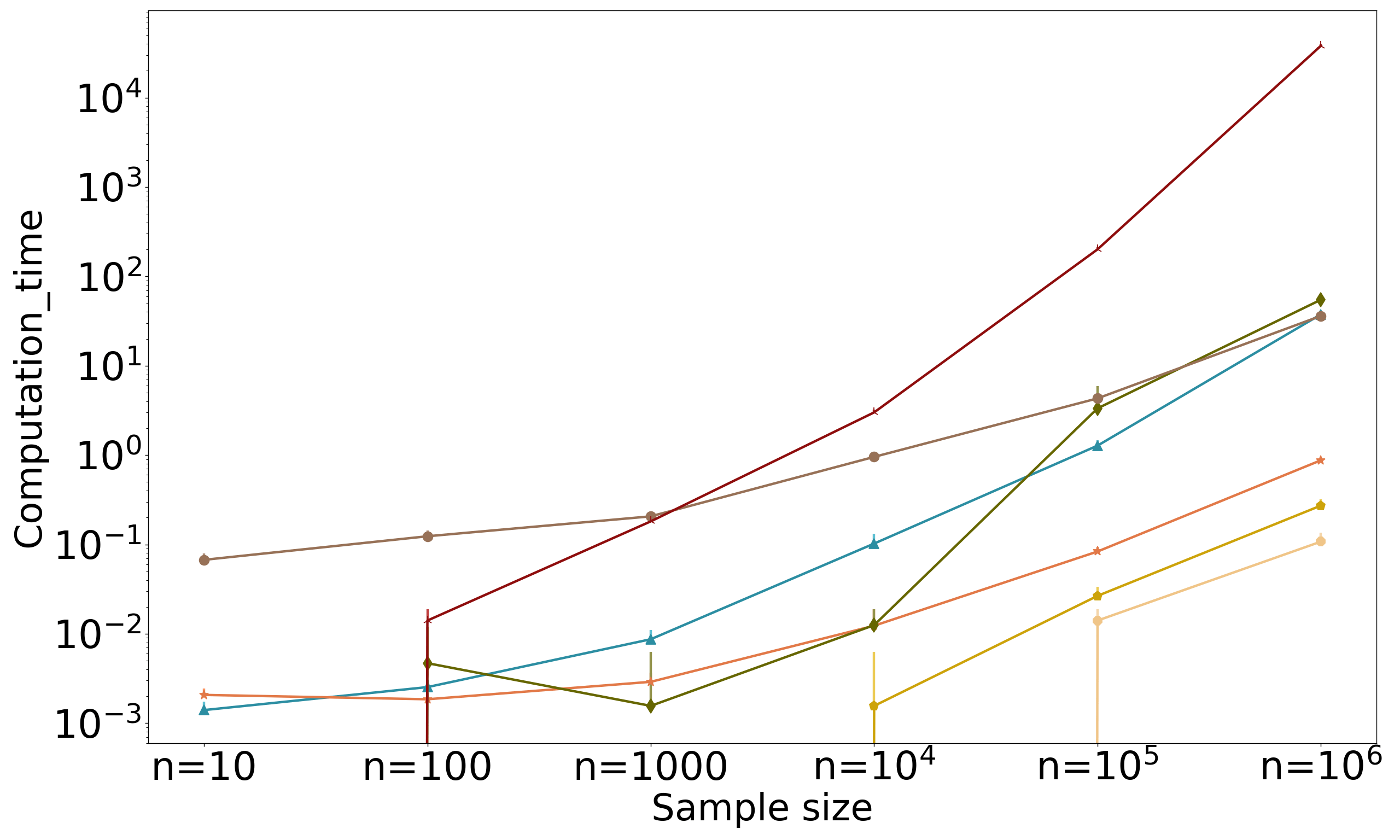
(b) Computation time,

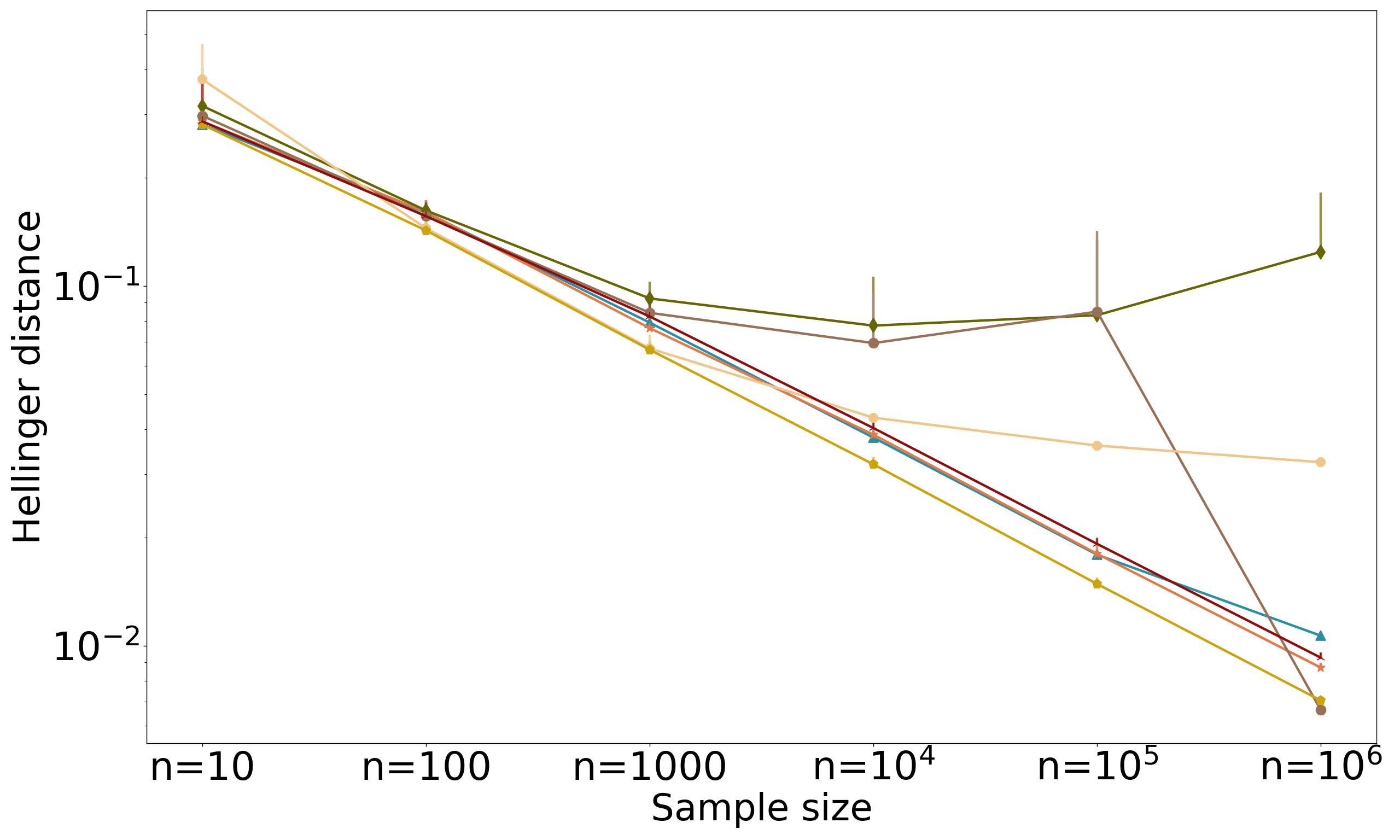
(c) Hellinger distance,

Figure 25: Different histograms obtained for a single mixture of 4 triangle distributions, of size $n=10^{4}$

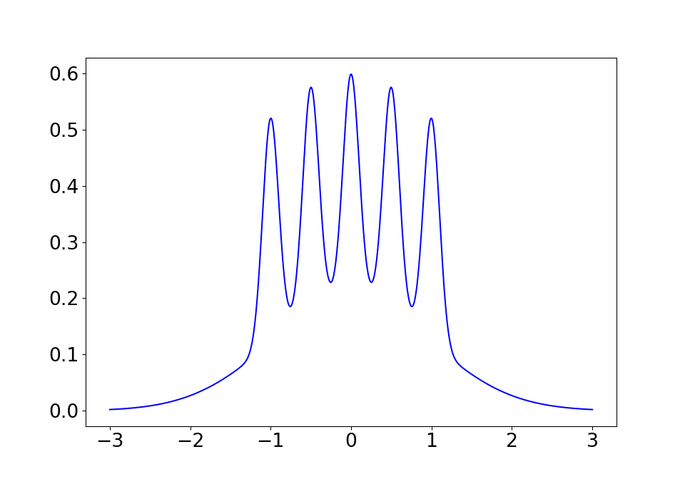
(a) Claw: a Gaussian mixture

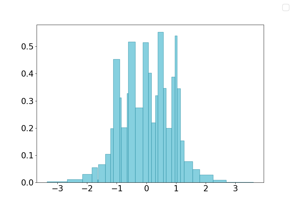
(b) NML + heuristic ($K^{*}=44$)

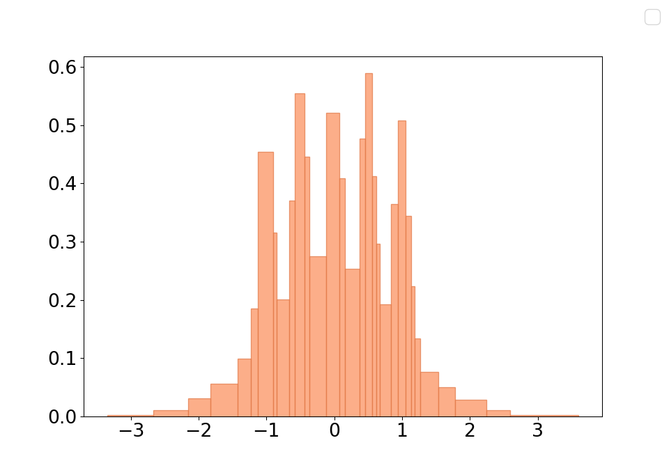
(c) G-Enum ($K^{*}=43$)

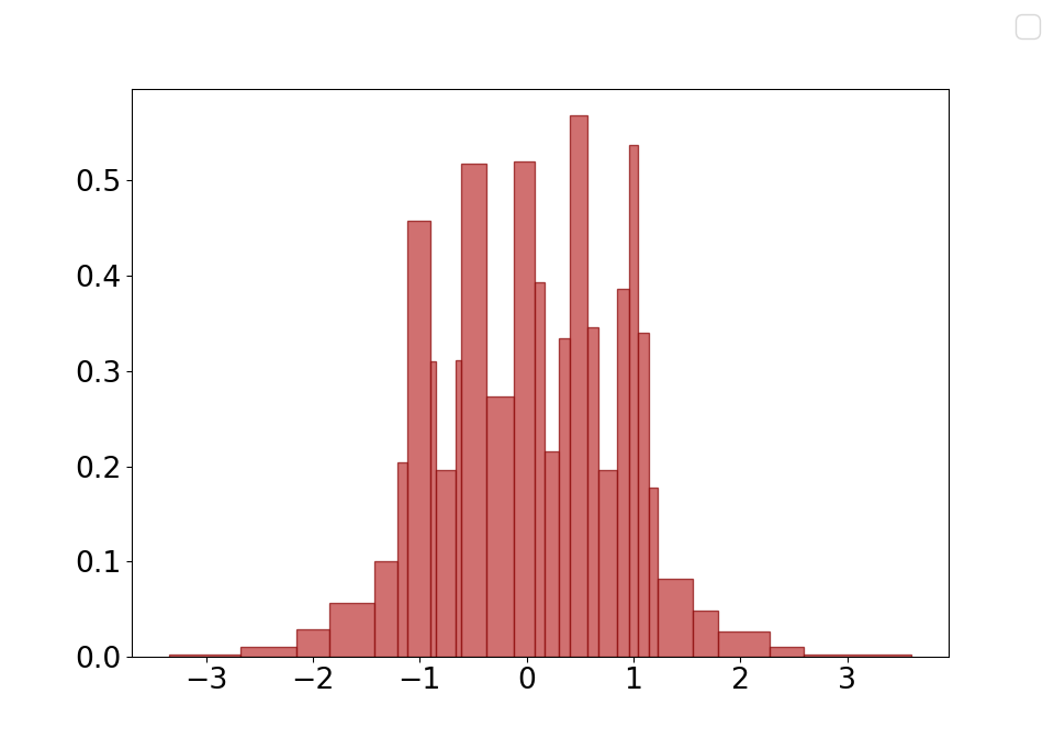
(d) Bayesian blocks ($K^{*}=46$)

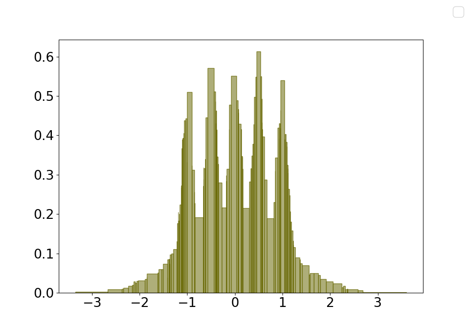
(e) Taut string ($K^{*}=205$)

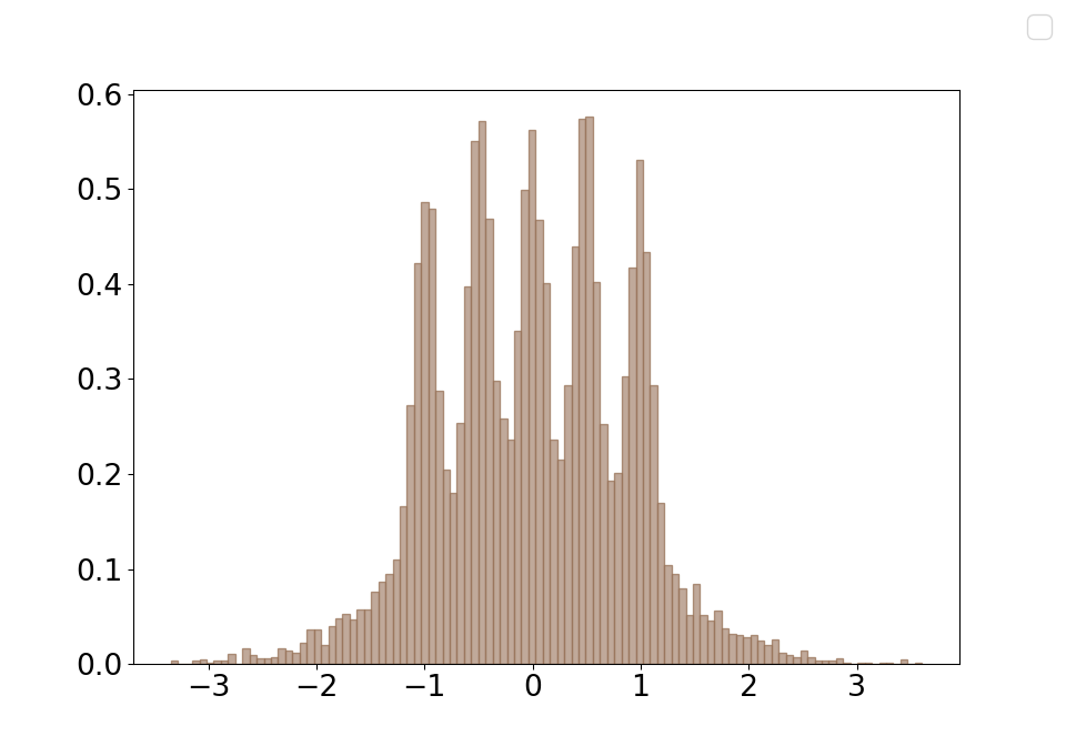
(f) RMG ($K^{*}=50$)

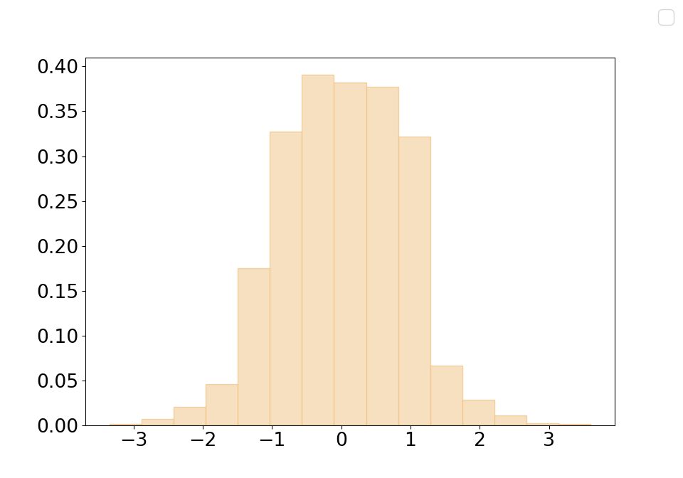
(g) Sturges ($K^{*}=15$)

(h) Freedman-Diaconis ($K^{*}=24$)

Figure 26: Comparison with state-of-the-art methods over the Claw Gaussian mixture of different sample sizes

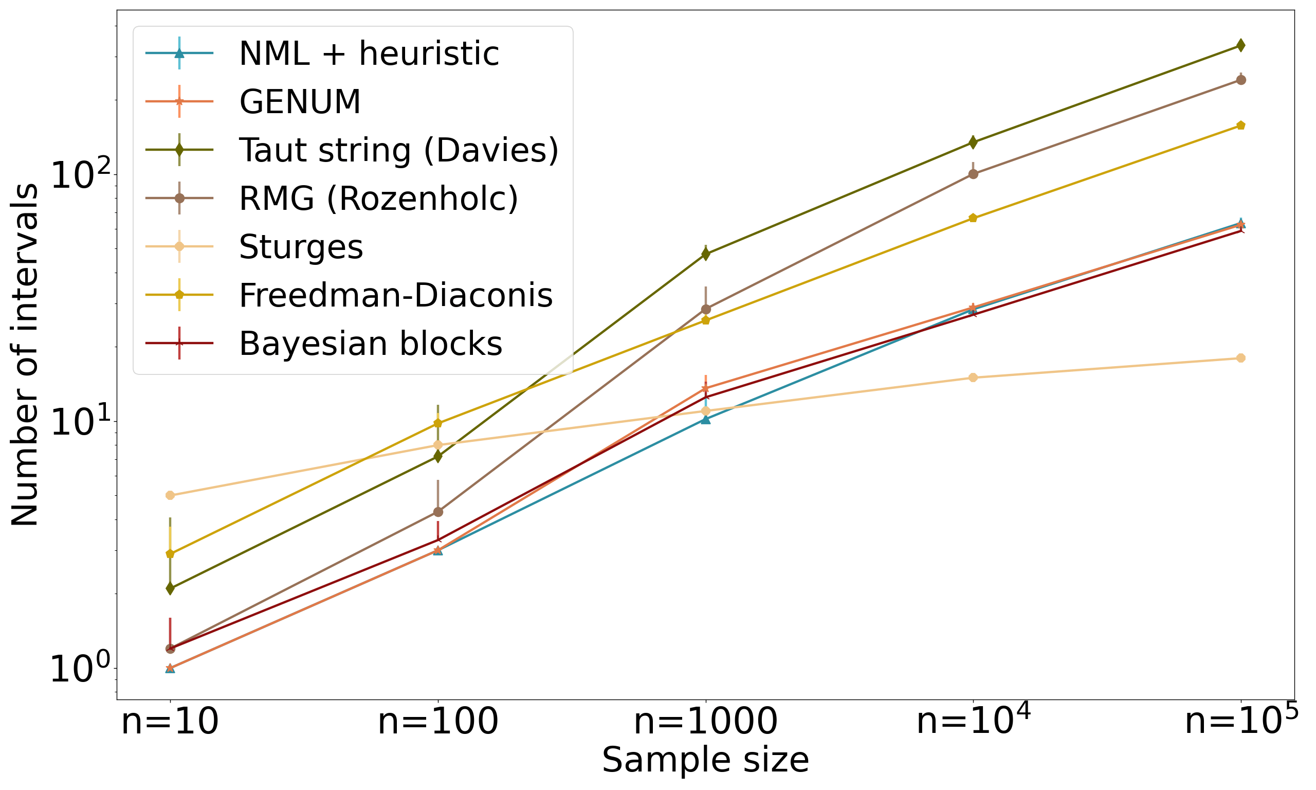
(a) Number of intervals,

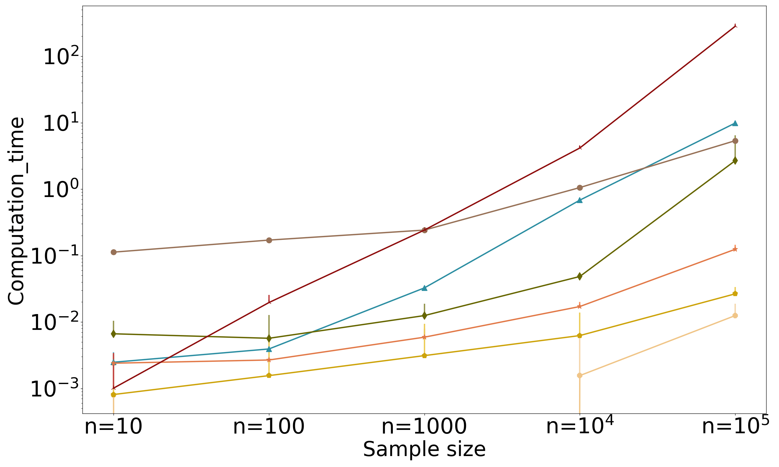
(b) Computation time,

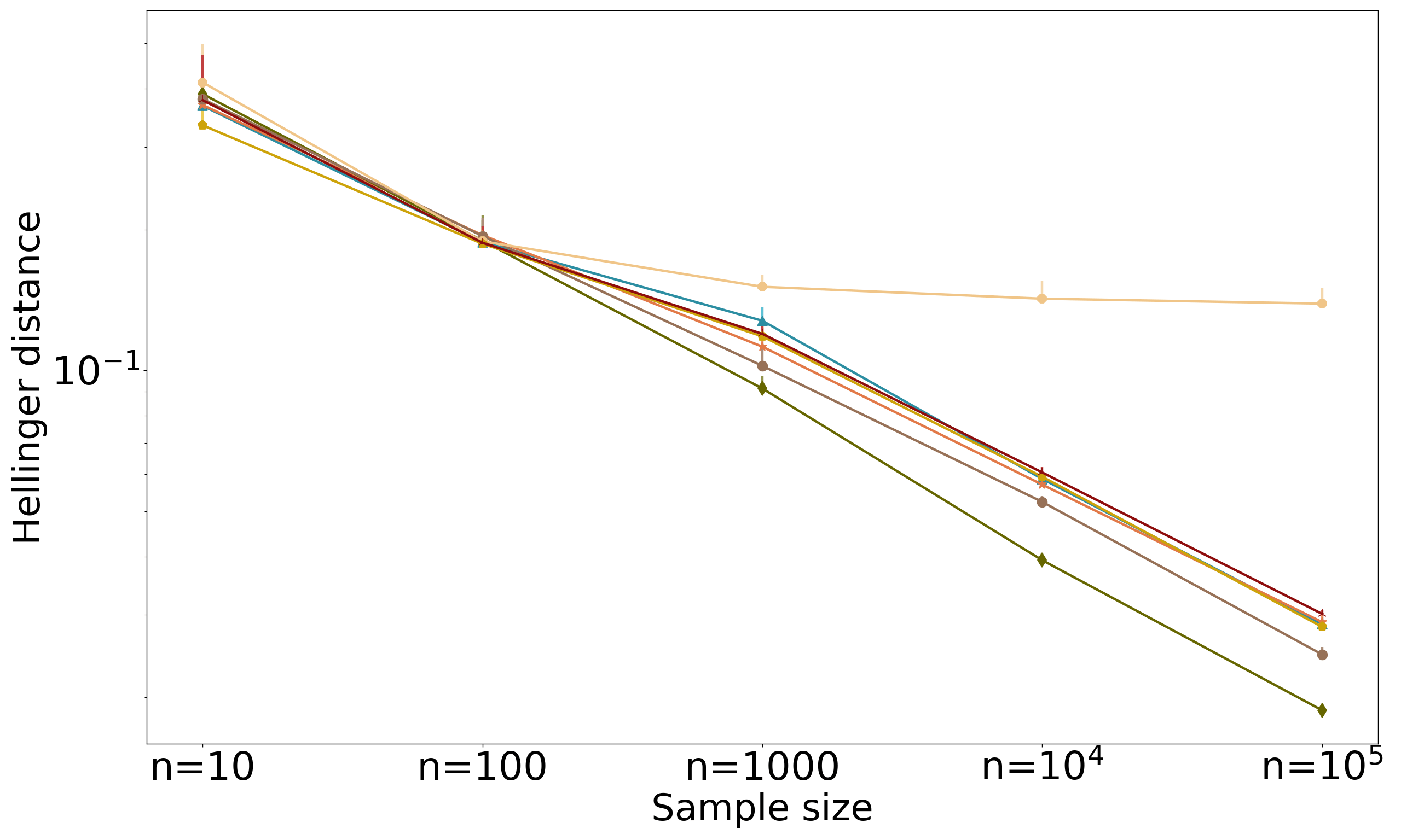
(c) Hellinger distance,

References

- Akaike (1998) Akaike, H., 1998. Information theory and an extension of the maximum likelihood principle, in: Parzen, E., Tanabe, K., Kitagawa, G. (Eds.), Selected Papers of Hirotugu Akaike. Springer New York, New York, NY, pp. 199–213. URL: https://doi.org/10.1007/978-1-4612-1694-0_15, doi:10.1007/978-1-4612-1694-0\_15.
- Astropy Collaboration et al. (2022) Astropy Collaboration, Price-Whelan, A.M., Lim, P.L., Earl, N., Starkman, N., Bradley, L., Shupe, D.L., Patil, A.A., Corrales, L., Brasseur, C.E., Nöthe, M., Donath, A., Tollerud, E., Morris, B.M., Ginsburg, A., Vaher, E., Weaver, B.A., Tocknell, J., Jamieson, W., van Kerkwijk, M.H., Robitaille, T.P., Merry, B., Bachetti, M., Günther, H.M., Aldcroft, T.L., Alvarado-Montes, J.A., Archibald, A.M., Bódi, A., Bapat, S., Barentsen, G., Bazán, J., Biswas, M., Boquien, M., Burke, D.J., Cara, D., Cara, M., Conroy, K.E., Conseil, S., Craig, M.W., Cross, R.M., Cruz, K.L., D’Eugenio, F., Dencheva, N., Devillepoix, H.A.R., Dietrich, J.P., Eigenbrot, A.D., Erben, T., Ferreira, L., Foreman-Mackey, D., Fox, R., Freij, N., Garg, S., Geda, R., Glattly, L., Gondhalekar, Y., Gordon, K.D., Grant, D., Greenfield, P., Groener, A.M., Guest, S., Gurovich, S., Handberg, R., Hart, A., Hatfield-Dodds, Z., Homeier, D., Hosseinzadeh, G., Jenness, T., Jones, C.K., Joseph, P., Kalmbach, J.B., Karamehmetoglu, E., Kałuszyński, M., Kelley, M.S.P., Kern, N., Kerzendorf, W.E., Koch, E.W., Kulumani, S., Lee, A., Ly, C., Ma, Z., MacBride, C., Maljaars, J.M., Muna, D., Murphy, N.A., Norman, H., O’Steen, R., Oman, K.A., Pacifici, C., Pascual, S., Pascual-Granado, J., Patil, R.R., Perren, G.I., Pickering, T.E., Rastogi, T., Roulston, B.R., Ryan, D.F., Rykoff, E.S., Sabater, J., Sakurikar, P., Salgado, J., Sanghi, A., Saunders, N., Savchenko, V., Schwardt, L., Seifert-Eckert, M., Shih, A.Y., Jain, A.S., Shukla, G., Sick, J., Simpson, C., Singanamalla, S., Singer, L.P., Singhal, J., Sinha, M., Sipőcz, B.M., Spitler, L.R., Stansby, D., Streicher, O., Šumak, J., Swinbank, J.D., Taranu, D.S., Tewary, N., Tremblay, G.R., Val-Borro, M.d., Van Kooten, S.J., Vasović, Z., Verma, S., de Miranda Cardoso, J.V., Williams, P.K.G., Wilson, T.J., Winkel, B., Wood-Vasey, W.M., Xue, R., Yoachim, P., Zhang, C., Zonca, A., Astropy Project Contributors, 2022. The Astropy Project: Sustaining and Growing a Community-oriented Open-source Project and the Latest Major Release (v5.0) of the Core Package. The Astrophysical Journal 935, 167. doi:10.3847/1538-4357/ac7c74, arXiv:2206.14220.
- Bellman (1961) Bellman, R., 1961. On the approximation of curves by line segments using dynamic programming. Communication of the ACM 4, 284.
- Birge and Rozenholc (2006) Birge, L., Rozenholc, Y., 2006. How many bins should be put in a regular histogram. ESAIM: Probability and Statistics 10, 24–45. URL: http://www.numdam.org/item/PS_2006__10__24_0, doi:10.1051/ps:2006001.
- Boullé (2006) Boullé, M., 2006. MODL: a Bayes optimal discretization method for continuous attributes. Machine Learning 65, 131–165.
- Boullé et al. (2016) Boullé, M., Clérot, F., Hue, C., 2016. Revisiting enumerative two-part crude MDL for Bernoulli and multinomial distributions (Extended version). Technical Report. arXiv, abs/1608.05522.
- Castellan (1999) Castellan, G., 1999. Modified Akaike’s criterion for histogram density estimation. Technical Report 61. Université Paris-Sud. Orsay. URL: https://www.imo.universite-paris-saclay.fr/~biblio/pub/1999/abs/ppo1999_61.html.
- Celisse (2014) Celisse, A., 2014. Optimal cross-validation in density estimation with the -loss. The Annals of Statistics 42, 1879 – 1910. URL: https://doi.org/10.1214/14-AOS1240, doi:10.1214/14-AOS1240.
- Celisse and Robin (2008) Celisse, A., Robin, S., 2008. Nonparametric density estimation by exact leave-p-out cross-validation. Computational Statistics & Data Analysis 52, 2350–2368. URL: https://www.sciencedirect.com/science/article/pii/S0167947307003842, doi:https://doi.org/10.1016/j.csda.2007.10.002.
- Davies et al. (2009) Davies, L.P., Gather, U., Nordman, D., Weinert, H., 2009. A comparison of automatic histogram constructions. ESAIM: PS 13, 181–196. URL: https://doi.org/10.1051/ps:2008005, doi:10.1051/ps:2008005.
- Davies and Kovac (2004) Davies, L.P., Kovac, A., 2004. Densities, spectral densities and modality. Ann. Statist. 32, 1093–1136. URL: https://doi.org/10.1214/009053604000000364, doi:10.1214/009053604000000364.
- Davies and Kovac (2012) Davies, L.P., Kovac, A., 2012. ftnonpar: Features and Strings for Nonparametric Regression. URL: https://CRAN.R-project.org/package=ftnonpar. R package version 0.1-88.
- Freedman and Diaconis (1981) Freedman, D., Diaconis, P., 1981. On the histogram as a density estimator:l2 theory. Zeitschrift für Wahrscheinlichkeitstheorie und Verwandte Gebiete 57, 453–476. URL: https://doi.org/10.1007/BF01025868, doi:10.1007/BF01025868.
- Grunwald (2007) Grunwald, P., 2007. The minimum description length principle. Adaptive computation and machine learning, MIT Press.
- Hall (1990) Hall, P., 1990. Akaike’s information criterion and Kullback-Leibler loss for histogram density estimation. Probability Theory and Related Fields 85, 449–467.
- Hall and Hannan (1988) Hall, P., Hannan, E.J., 1988. On stochastic complexity and nonparametric density estimation. Biometrika 75, 705–714. URL: http://www.jstor.org/stable/2336311.
- Harris et al. (2020) Harris, C.R., Millman, K.J., van der Walt, S.J., Gommers, R., Virtanen, P., Cournapeau, D., Wieser, E., Taylor, J., Berg, S., Smith, N.J., Kern, R., Picus, M., Hoyer, S., van Kerkwijk, M.H., Brett, M., Haldane, A., del Río, J.F., Wiebe, M., Peterson, P., Gérard-Marchant, P., Sheppard, K., Reddy, T., Weckesser, W., Abbasi, H., Gohlke, C., Oliphant, T.E., 2020. Array programming with NumPy. Nature 585, 357–362. URL: https://doi.org/10.1038/s41586-020-2649-2, doi:10.1038/s41586-020-2649-2.
- Ioannidis (2003) Ioannidis, Y., 2003. The history of histograms (abridged), in: Freytag, J.C., Lockemann, P., Abiteboul, S., Carey, M., Selinger, P., Heuer, A. (Eds.), Proceedings 2003 VLDB Conference. Morgan Kaufmann, San Francisco, pp. 19–30. URL: https://www.sciencedirect.com/science/article/pii/B9780127224428500112, doi:https://doi.org/10.1016/B978-012722442-8/50011-2.
- Kanazawa (1988) Kanazawa, Y., 1988. An optimal variable cell histogram. Communications in Statistics - Theory and Methods 17, 1401–1422. URL: https://doi.org/10.1080/03610928808829688, doi:10.1080/03610928808829688, arXiv:https://doi.org/10.1080/03610928808829688.
- Knuth (2019) Knuth, K.H., 2019. Optimal data-based binning for histograms and histogram-based probability density models. Digital Signal Processing 95, 102581. URL: https://www.sciencedirect.com/science/article/pii/S1051200419301277, doi:https://doi.org/10.1016/j.dsp.2019.102581.
- Knuth et al. (2006) Knuth, K.H., Castle, J.P., Wheeler, K.R., 2006. Identifying excessively rounded or truncated data, in: Rizzi, A., Vichi, M. (Eds.), Compstat 2006 - Proceedings in Computational Statistics, Physica-Verlag HD, Heidelberg. pp. 313–323.
- Kontkanen (2009) Kontkanen, P., 2009. Computationally efficient methods for MDL-optimal density estimation and data clustering. Department of Computer Science, series of publications A, report, 2009-11, University of Helsinki.
- Kontkanen et al. (2003) Kontkanen, P., Buntine, W.L., Myllymäki, P., Rissanen, J., Tirri, H., 2003. Efficient computing of stochastic complexity, in: Bishop, C.M., Frey, B.J. (Eds.), Proceedings of the Ninth International Workshop on Artificial Intelligence and Statistics, PMLR. pp. 171–178. URL: https://proceedings.mlr.press/r4/kontkanen03a.html. reissued by PMLR on 01 April 2021.
- Kontkanen and Myllymäki (2007) Kontkanen, P., Myllymäki, P., 2007. A linear-time algorithm for computing the multinomial stochastic complexity. Inf. Process. Lett. 103, 227–233. URL: https://doi.org/10.1016/j.ipl.2007.04.003, doi:10.1016/j.ipl.2007.04.003.
- Kontkanen and Myllymäki (2007) Kontkanen, P., Myllymäki, P., 2007. Mdl histogram density estimation, in: Meila, M., Shen, X. (Eds.), Proceedings of the Eleventh International Conference on Artificial Intelligence and Statistics, PMLR, San Juan, Puerto Rico. pp. 219–226.
- Li et al. (2020) Li, H., Munk, A., Sieling, H., Walther, G., 2020. The essential histogram. Biometrika 107, 347–364. URL: https://doi.org/10.1093/biomet/asz081, doi:10.1093/biomet/asz081, arXiv:https://academic.oup.com/biomet/article-pdf/107/2/347/33218017/asz081.pdf.
- Luosto et al. (2012) Luosto, P., Giurcaneanu, C., Kontkanen, P., 2012. Construction of irregular histograms by penalized maximum likelihood: a comparative study, in: Information Theory Workshop (ITW), IEEE Computer Society, United States. pp. 297–301. doi:10.1109/ITW.2012.6404679. volume: Proceeding volume:.
- Mildenberger et al. (2019) Mildenberger, T., Rozenholc, Y., Zasada, D., 2019. histogram: Construction of Regular and Irregular Histograms with Different Options for Automatic Choice of Bins. URL: https://CRAN.R-project.org/package=histogram. R package version 0.0-25.
- Minton et al. (2019) Minton, D.A., Fassett, C.I., Hirabayashi, M., Howl, B.A., Richardson, J.E., 2019. The equilibrium size-frequency distribution of small craters reveals the effects of distal ejecta on lunar landscape morphology. Icarus 326, 63 – 87. doi:https://doi.org/10.1016/j.icarus.2019.02.021.
- Mononen and Myllymäki (2008) Mononen, T., Myllymäki, P., 2008. Computing the multinomial stochastic complexity in sub-linear time, in: Proceedings of the 4th European Workshop on Probabilistic Graphical Models (PGM-08), September 17-19, 2008, Hirtshals, Denmark, pp. 209–216. Volume: Proceeding volume:.
- Oommen and Rueda (2002) Oommen, B.J., Rueda, L.G., 2002. The Efficiency of Histogram-like Techniques for Database Query Optimization. The Computer Journal 45, 494–510. URL: https://doi.org/10.1093/comjnl/45.5.494, doi:10.1093/comjnl/45.5.494, arXiv:https://academic.oup.com/comjnl/article-pdf/45/5/494/1198482/450494.pdf.
- Rissanen (1978) Rissanen, J., 1978. Modeling by shortest data description. Automatica 14, 465–471. doi:10.1016/0005-1098(78)90005-5.
- Rissanen (1983) Rissanen, J., 1983. A universal prior for integers and estimation by minimum description length. Ann. Statist. 11, 416–431. doi:10.1214/aos/1176346150.
- Rissanen (1986) Rissanen, J., 1986. Stochastic complexity and modeling. The Annals of Statistics 14, 1080–1100. URL: http://www.jstor.org/stable/3035559.
- Rissanen (2001) Rissanen, J., 2001. Strong optimality of the normalized ml models as universal codes and information in data. IEEE Transactions on Information Theory 47, 1712–1717.
- Rissanen et al. (1992) Rissanen, J., Speed, T.P., Yu, B., 1992. Density estimation by stochastic complexity. IEEE Transactions on Information Theory 38, 315–323. doi:10.1109/18.119689.
- Robbins (2019) Robbins, S.J., 2019. A new global database of lunar impact craters 1–2 km: 1. crater locations and sizes, comparisons with published databases, and global analysis. Journal of Geophysical Research: Planets 124, 871–892. doi:10.1029/2018JE005592.
- Rozenholc et al. (2010) Rozenholc, Y., Mildenberger, T., Gather, U., 2010. Combining regular and irregular histograms by penalized likelihood. Computational Statistics and Data Analysis 54, 3313 – 3323. URL: http://www.sciencedirect.com/science/article/pii/S0167947310001660, doi:https://doi.org/10.1016/j.csda.2010.04.021.
- Rudemo (1982) Rudemo, M., 1982. Empirical choice of histograms and kernel density estimators. Scandinavian Journal of Statistics 9, 65–78. URL: http://www.jstor.org/stable/4615859.
- Scargle et al. (2013) Scargle, J.D., Norris, J.P., Jackson, B., Chiang, J., 2013. Studies in Astronomical Time Series Analysis. VI. Bayesian Block Representations. Astrophysical Journal 764, 167. doi:10.1088/0004-637X/764/2/167, arXiv:1207.5578.
- Schwarz (1978) Schwarz, G., 1978. Estimating the Dimension of a Model. The Annals of Statistics 6, 461 – 464. URL: https://doi.org/10.1214/aos/1176344136, doi:10.1214/aos/1176344136.
- Scott (1979) Scott, D.W., 1979. On optimal and data based histograms. Biometrika 66, 605–610.
- Shtarkov (1987) Shtarkov, Y.M., 1987. Universal sequential coding of individual messages. Problems of Information Transmission 23, 3–17.
- Sturges (1926) Sturges, H.A., 1926. The choice of a class interval. Journal of the American Statistical Association 21, 65–66. URL: https://doi.org/10.1080/01621459.1926.10502161, doi:10.1080/01621459.1926.10502161, arXiv:https://doi.org/10.1080/01621459.1926.10502161.
- Sulewski (2020) Sulewski, P., 2020. Equal-bin-width histogram versus equal-bin-count histogram. Journal of Applied Statistics 0, 1–20. URL: https://doi.org/10.1080/02664763.2020.1784853, doi:10.1080/02664763.2020.1784853, arXiv:https://doi.org/10.1080/02664763.2020.1784853.
- Szpankowski (1998) Szpankowski, W., 1998. On asymptotics of certain recurrences arising in universal coding. Problems of Information Transmission 34, 142–146.
- Taylor (1987) Taylor, C.C., 1987. Akaike’s information criterion and the histogram. Biometrika 74, 636–639. URL: http://www.jstor.org/stable/2336704.
- Wand (1997) Wand, M.P., 1997. Data-based choice of histogram bin width. The American Statistician 51, 59–64. URL: http://www.jstor.org/stable/2684697.
- Wang and Zhou (2016) Wang, N., Zhou, J.L., 2016. Determining proportions of lunar crater populations by fitting crater size distribution. Research in Astronomy and Astrophysics 16, 185. doi:10.1088/1674-4527/16/12/185.
- Zubiaga and Mac Namee (2016) Zubiaga, A., Mac Namee, B., 2016. Graphical perception of value distributions: An evaluation of non-expert viewers’ data literacy. Journal of Community Informatics 12. doi:10.15353/joci.v12i3.3282. special Issue on Data Literacy.