On the asymptotics of extremal $\ell^{p}$-blocks cluster inference

Abstract.

Extremes occur in stationary regularly varying time series as short periods with several large observations, known as extremal blocks. We study cluster statistics summarizing the behavior of functions acting on these extremal blocks. Examples of cluster statistics are the extremal index, cluster size probabilities, and other cluster indices. The purpose of our work is twofold. First, we state the asymptotic normality of block estimators for cluster inference based on consecutive observations with large $\ell^{p}$-norms, for $p>0$. The case $p={\alpha}$, where ${\alpha}>0$ is the tail index of the time series, has specific nice properties thus we analyze the asymptotic of blocks estimators when approximating ${\alpha}$ using the Hill estimator. Second, we verify the conditions we require on classical models such as linear models and solutions of stochastic recurrence equations. Regarding linear models, we prove that the asymptotic variance of classical index cluster-based estimators is null as first conjectured in [28]. We illustrate our findings on simulations.

1. Introduction

We study stationary heavy-tailed time series $(\mathbf{X}_{t})$ in $(\mathbb{R}^{d},|\cdot|)$, with regularly varying distributions, and tail index $\alpha>0$; cf. [5], a formal definition is conferred to Section 2.2. In this framework, extremal observations cluster: an extreme value triggers a short period with numerous large observations. This behavior is known to perturb classical inference procedures tailored for independent observations like high quantile inference; see [22]. This clustering effect can be summarized with the extremal index, initially introduced in [38] and [39]. We can interpret it as the inverse of the mean number of consecutive exceedances above a high threshold in a short period of time. In this article, we aim to infer statistics of the clustering effect by letting functionals act on consecutive observations with extremal behavior. For example, we can recover the extremal index from this setting and also other important indices of the extremes of the series.

For extremal cluster inference, we consider a sample $\mathbf{X}_{[1,n]}$ together with a sequence $(b_{n})$, and we define the sample of disjoint blocks $(\mathcal{B}_{j})_{j=1,\dots,m_{n}}$ as blocks of consecutive observations:

(1.1) $$\mathcal{B}_{j} := (\mathbf{X}_{(j-1)b_{n}+1},\dots,\mathbf{X}_{jb_{n}})\;=\;\mathbf{X}_{(j-1)b_{n}+[1,b_{n}]},$$

such that $b_{n}\to\infty$, $m_{n}=n/b_{n}\to\infty$, as $n\to\infty$. Following the $p$-clusters theory developed in [12], the extremal behavior of the series is modeled by the $p$-clusters which we can recover form the conditional behavior of a block $\mathcal{B}_{j}$ given that its ${\ell}^{p}-$norm is large:

$${\mathbb{P}}(\mathcal{B}_{1}/x_{b_{n}}\in A\,|\,\|\mathcal{B}_{1}\|_{p}>x_{b_{n}}) \xrightarrow[]{w} {\mathbb{P}}(Y{\bf Q}^{(p)}\in A\,),\qquad n\to\infty,$$

such that $Y$ is independent of ${\bf Q}^{(p)}\in{\ell}^{p}$, ${\mathbb{P}}(Y>y)=y^{-\alpha},$ for $y>1$, and $\|{\bf Q}^{(p)}\|_{p}=1$ a.s., for $p\in(0,\infty]$. The weak convergence holds for a family of shift-invariant continuity sets $A\subset\ell^{p}$, and $(x_{n})$ is a suitable sequence satisfying ${\mathbb{P}}(\|\mathcal{B}_{1}\|_{p}>x_{b_{n}})\to 0$, as $n\to\infty$.

In this article we study inference of $p$-cluster statistics of the form

(1.2) $$\quad f^{{\bf Q}}(p) = {\mathbb{E}}[f(Y{\bf Q}^{(p)})]\,,$$

for suitable $\ell^{p}$-continuity functions $f:\ell^{p}\to\mathbb{R}$ which are invariant to the shift operator of sequences. To infer the cluster statistic (1.2), we use the disjoint blocks estimators proposed in [12], and defined as

(1.3) $$\widehat{f^{\bf Q}}(p) := \frac{1}{k}\sum_{t=1}^{m_{n}}f({\mathcal{B}}_{t}/\|{\mathcal{B}}\|_{p,(k+1)})\mathrm{1}\mathrm{1}(\|{\mathcal{B}}_{t}\|_{p}>\|{\mathcal{B}}\|_{p,(k+1)}),$$

where $\|{\mathcal{B}}\|_{p,(1)}\geqslant\|{\mathcal{B}}\|_{p,(2)}\geqslant\dots\geqslant\|{\mathcal{B}}\|_{p,(m_{n})},$ denotes the sequence of order statistics of the $\ell^{p}-$norms of blocks defined in (1.1). Examples of cluster statistics are the extremal index, and other important cluster indices.

The case $p={\alpha}$ is particularly relevant for two reasons. First, the $\ell^{\alpha}$-norm’s tail ${\mathbb{P}}(\|\mathcal{B}_{1}\|_{\alpha}>x_{b_{n}})$ is equivalent to $b_{n}{\mathbb{P}}(|\mathbf{X}_{1}|>x_{b_{n}})$, which is the tail of any $\ell^{p}-$norm of blocks in the iid case. Thus the choice $p=\alpha$ is ideal for tuning the parameters in the blocks estimator as it is less susceptible to local serial dependencies; see [12] for a discussion on that topic. Second, under mixing and anti-clustering conditions, choosing $(a_{n})$ satisfying $n\,{\mathbb{P}}(|\mathbf{X}_{1}|>a_{n})\to 1$ as $n\to\infty$, [13] prove that

(1.4) $$\sum_{t=1}^{n}\varepsilon_{a_{n}^{-1}\mathbf{X}_{t}} \stackrel{{\scriptstyle d}}{{\rightarrow}} \sum_{i=1}^{\infty}\sum_{j=-\infty}^{\infty}\varepsilon_{\Gamma_{i}^{-1/{\alpha}}{\bf Q}_{ij}}\,,\qquad n\to\infty\,,$$

where $(\Gamma_{i})$ are the points of an homogeneous Poisson process, $({\bf Q}_{ij})_{j}$ are independent copies of the ${\alpha}-$cluster process ${\bf Q}:={\bf Q}^{({\alpha})}$ independent of $(\Gamma_{i})$. Thus the extremal cluster dependencies of the series are fully modeled using the spectral cluster process ${\bf Q}$, and from it one can recover the distribution of ${\bf Q}^{(p)}$, for every $p\in(0,\infty]$ using the change-of-norms equation given by [12] and recalled in (2.12). This means in general we can estimate $p$-cluster statistics using $\ell^{\alpha}-$blocks estimators.

The main goal of this article is to establish the asymptotic normality of the blocks estimators from Equation (1.3), tailored for cluster inference. We state moment, mixing and bias assumptions yielding the existence of a sequence $(k_{n})$, satisfying $k=k_{n}\to\infty$, $m_{n}/k_{n}\to\infty$ such that

(1.5) $$\sqrt{k}\big{(}\,\widehat{f^{\bf Q}}(p)-f^{\bf Q}(p)\,\big{)} \xrightarrow[]{d} \mathcal{N}\big{(}0,{\rm Var}(f(Y{\bf Q}^{(p)}))\,\big{)}\,,\quad n\to\infty,$$

and the limit is a centered Gaussian distribution. Our inference methodology can be viewed as a Peak Over Threshold over order statistics of blocks. Moreover, for $p={\alpha}$, fixing $k$ and letting first $n\to\infty$ in (1.3), we see from (1.4)

$$\widehat{f^{\bf Q}}({\alpha}) \approx \frac{1}{k}\sum_{i=1}^{k}f((\Gamma_{i}/\Gamma_{k+1})^{-1/{\alpha}}({{\bf Q}}_{it})_{t})\,.$$

Then, the simple expression of the asymptotic variance follows as $(\Gamma_{i}/\Gamma_{k+1})\stackrel{{\scriptstyle d}}{{=}}(U_{k,i})$ where $U_{k,1}<\cdots<U_{k,k}$ are the ordered statistics of iid uniformly distributed $U_{j}$, $1\leqslant j\leqslant k$, and $U^{-1/{\alpha}}\stackrel{{\scriptstyle d}}{{=}}Y$. This heuristic is extended to any $p-$cluster ${{\bf Q}}^{(p)}$, $p\in(0,\infty]$, via the change-of-norms in (2.12).

In general for $p$-cluster inference, the function $f(p)$ can involve the tail-index $\alpha$ in its expression, meaning $f(p)=f_{\alpha}(p)$. Furthermore, we already mentioned that the choice of $p=\alpha$ has some advantages, thus to implement these procedures we need to replace $\alpha$ with an estimate $\widehat{\alpha}$. We then show the asymptotic normality of $p$–cluster estimators of $f_{\widehat{\alpha}}(p)$ when we let $1/\widehat{\alpha}$ equal the classical Hill estimator, and we extend the analysis to cover ${\widehat{\alpha}}$–cluster inference. Furthermore, we conduct simulations to illustrate that $\ell^{\widehat{\alpha}}$–block estimators are competitive both in terms of bias and variance for finite sample sizes.

Our asymptotic results highlight how introducing $\ell^{p}-$norm block order statistics in (1.3), instead of order statistics of the sample $(|\mathbf{X}_{t}|)$ as in [20, 14], can lead to a better asymptotic variance for cluster inference. We give examples of variance reduction in the case of linear models with short-range dependence, for inference of classical indices. In our examples, the asymptotic variance of linear models ${\rm Var}(f(Y{\bf Q}^{(p)}))$ is null because of the deterministic properties of the spectral $p$-cluster process of linear models. For linear models, the advantage of replacing thresholds with block maxima records was previously investigated in [28]. Existing works [18, 20, 14, 37] following [28] focus on cluster of exceedances inference such that $p=\infty$. Our asymptotic result comforts and extends the heuristics presented in [28] for $p=\infty$ and linear models to the case $p<\infty$ and general models. To prove the asymptotic normality of block estimators, we rely on the theory of empirical processes [53], but adapted to block estimators. For this purpose, we build on the previous work of [18], and the modern overview in [37]. To handle the asymptotics of extremal $\ell^{p}$-blocks, we build on the large deviation principles studied in [12], and appeal to the $p$-cluster processes theory therein.

The article is organized as follows. Preliminaries on mixing coefficients, regular variation, and the $p$-cluster theory of stationary time series are compiled in Section 2. In Section 3 we present our main result in Theorem 3.1, stating the asymptotic normality of the block estimators introduced in Equation (1.3). We work under mixing, moment, and bias conditions on the series that we also present in Section 3. Section 4 studies examples of extremal cluster inference such as estimation of the extremal index, the cluster size probabilities, and the cluster index for sums. We conclude by verifying our conditions on classical models such as linear processes and stochastic recurrence equations in Section 5. In the case of linear models with short-range dependence, Theorem 5.6 states that the $\ell^{p}$-block estimators of all the aforementioned quantities have null-asymptotic variance. Thereby, they are super-efficient for cluster inference of important indices as conjectured by [28] for $p=\infty$. We illustrate the finite-sample performances of our estimators in Section 6. All proofs are deferred to Apendices A, B, C.

1.1. Notation

We consider stationary time series $(\mathbf{X}_{t})$ taking values in $\mathbb{R}^{d}$, that we endow with a norm $|\cdot|$. Let $p>0$, and $({\bf x}_{t})\in(\mathbb{R}^{d})^{\mathbb{Z}}$. Define the $p$-modulus function $\|\cdot\|_{p}:(\mathbb{R}^{d})^{\mathbb{Z}}\to[0,\infty]$ as

$$\|({\bf x}_{t})\|^{p}_{p} := \sum_{t\in\mathbb{Z}}|{\bf x}_{t}|^{p}\,,$$

and define the sequential space $\ell^{p}$ as $\ell^{p}:=\{({\bf x}_{t})\in(\mathbb{R}^{d})^{\mathbb{Z}}:\|({\bf x}_{t})\|_{p}^{p}<\infty\}\,,$ with the convention that, for $p=\infty$, the space $\ell^{\infty}$ refers to sequences with finite supremum norm. For any $p\in(0,\infty]$, the $p$-modulus functions induce a distance $d_{p}$ in $\ell^{p}$, and for $p\in[1,\infty)$, it defines a norm. Abusing notation, we call them all $\ell^{p}$-norms. Let $\tilde{\ell}^{p}=\ell^{p}/\sim$ be the shift-invariant quotient space where: $({\bf x}_{t})\sim({\bf y}_{t})$ if and only if there exists $k\in\mathbb{Z}$ such that ${\bf x}_{t-k}={\bf y}_{t}$, $t\in\mathbb{Z}$. We also consider the metric space $(\tilde{\ell}^{p},\tilde{d}_{p})$ such that for $[{\bf x}],[{\bf y}]\in\tilde{\ell}^{p}$,

$$\tilde{d}_{p}([{\bf x}],[{\bf y}]) := \inf_{k\in\mathbb{Z}}\{d_{p}({\bf x}_{t-k},{\bf y}_{t}),({\bf x}_{t})\in[{\bf x}],({\bf y}_{t})\in[{\bf y}]\},$$

and without loss of generality, we write an element $[{\bf x}]$ in $\tilde{\ell}^{p}$ also as $({\bf x}_{t})$. Further details on the shift-invariant spaces are deferred to [12, 4].

The operator norm for $d\times d$ matrices, ${{\bf A}}\in\mathbb{R}^{d\times d}$, is defined as $|{{\bf A}}|_{op}:=\sup_{|{\bf x}|=1}|{\bf A}{\bf x}|.$ The truncation operations of $({\bf x}_{t})$ at the level $\epsilon$, for $\epsilon>0$, are defined by

$$(\overline{{\bf x}}_{t}^{\varepsilon}) := ({\bf x}_{t}\mathrm{1}\mathrm{1}_{|{\bf x}_{t}|\leqslant\varepsilon})\,,\qquad\qquad(\underline{{\bf x}_{t}}_{\epsilon})\;:=\;({\bf x}_{t}\mathrm{1}\mathrm{1}_{|{\bf x}_{t}|>\varepsilon})\,.$$

The notation $a\land b$ denotes the minimum between two constants $a,b\in\mathbb{Z}$, and $a\lor b$ denotes its maximum. We write $\log^{+}(x):=\log(x)\lor 0$, for $x\in(0,\infty)$. We sometimes write ${\bf x}$ for the sequence ${\bf x}:=({\bf x}_{t})\in(\mathbb{R}^{d})^{\mathbb{Z}}$. Furthermore, for $a,b,\in\mathbb{R}$, and $a\leqslant b$, we write as ${\bf x}_{[a,b]}$ the vector $({\bf x}_{t})_{t=a,\dots,b}$ taking values in $(\mathbb{R}^{d})^{b-a+1}$. We write ${\bf x}_{[a,b]}\in\tilde{\ell}^{p}$, which means we take the natural embedding of ${\bf x}_{[a,b]}$ in $\tilde{\ell}^{p}$ defined by assigning zeros to undefined coefficients. It will be convenient to write $\mathcal{G}_{+}(\tilde{\ell}^{p})$ for the continuous non-negative functions on $(\tilde{\ell}^{p},\tilde{d}_{p})$ which vanish in a neighborhood of the origin.

2. Preliminaries

2.1. Mixing coefficients

Let $(\mathbf{X}_{t})$ be an $\mathbb{R}^{d}$-valued strictly stationary time series defined over a probability space $((\mathbb{R}^{d})^{\mathbb{Z}},\mathcal{A},{\mathbb{P}})$. The properties of stationary sequences are usually studied through mixing coefficients. Denote the past and future $\sigma-$algebras by

$$\mathcal{F}_{t\leqslant 0}\quad:=\quad\sigma((\mathbf{X}_{t})_{t\leqslant 0}),\qquad\mathcal{F}_{t\geqslant h}\quad:=\quad\sigma((\mathbf{X}_{t})_{t\geqslant h}),\qquad h\geqslant 1\,,$$

respectively. We recall the definition of the mixing coefficients $(\beta_{h})$ below

$$\beta_{h} := d_{TV}\big{(}\,{\mathbb{P}}_{\mathcal{F}_{t\leqslant 0}\otimes\mathcal{F}_{t\geqslant h}}\,,\,{\mathbb{P}}_{\mathcal{F}_{t\leqslant 0}}\otimes{\mathbb{P}}_{\mathcal{F}_{t\geqslant h}}\,\big{)},$$

where $d_{TV}(\cdot,\cdot)$ is the total variation distance between two probability measures: $((\mathbb{R}^{d})^{\mathbb{Z}},\mathcal{A},{\mathbb{P}}_{1})$, $((\mathbb{R}^{d})^{\mathbb{Z}},\mathcal{A},{\mathbb{P}}_{2})$, and ${\mathbb{P}}_{1}\otimes{\mathbb{P}}_{2}(A\times B):={\mathbb{P}}_{1}(A){\mathbb{P}}_{2}(B),$ for $A,B\in\mathcal{A}$. For a summary on mixing conditions see [8, 17, 46].

Remark 2.1.

A detailed interpretation of the $\beta-$mixing coefficients $(\beta_{h})$ in terms of the total variation distance can be found in Chapter 1.2 in [17]. These mixing coefficients are well adapted while working with Markov processes. Indeed, a strictly stationary Harris recurrent Markov chain $(\mathbf{X}_{t})$, satisfies $\beta_{t}\to 0$ exponentially fast as $t\to\infty$; see Theorem 3.5 in [8].

2.2. Regular variation

We consider stationary time series $(\mathbf{X}_{t})$ taking values in $(\mathbb{R}^{d},|\cdot|)$ and regularly varying with tail index $\alpha>0$: all its finite-dimensional vectors are multivariate regularly varying of the same index. In this case we write $(\mathbf{X}_{t})$ satisfies $\bf RV_{\alpha}$. Borrowing the ideas in [5], $(\mathbf{X}_{t})$ satisfies $\bf RV_{\alpha}$ if and only if, for all $h\geqslant 0$, there exists a vector $(\mbox{$\boldsymbol{\Theta}$}_{t})_{|t|\leqslant h}$, taking values in $(\mathbb{R}^{d})^{2h+1}$ such that

(2.6) $${\mathbb{P}}(x^{-1}(\mathbf{X}_{t})_{|t|\leqslant h}\in\cdot\,|\,|\mathbf{X}_{0}|>x) \xrightarrow[]{d} {\mathbb{P}}(Y(\mbox{$\boldsymbol{\Theta}$}_{t})_{|t|\leqslant h}\in\cdot),\quad x\to\infty,$$

where $Y$ is independent of $(\mbox{$\boldsymbol{\Theta}$}_{t})_{|t|\leqslant h}$ and ${\mathbb{P}}(Y>y)=y^{-\alpha},y>1$. We call the sequence $(\mbox{$\boldsymbol{\Theta}$}_{t})$, taking values in $(\mathbb{R}^{d})^{\mathbb{Z}}$, the spectral tail process.

The time series $(\mbox{$\boldsymbol{\Theta}$}_{t})$ does not inherit the stationarity property of the series. Instead, the time-change formula of [5] holds: for any $s,t\in\mathbb{Z},s\leqslant 0\leqslant t$ and for any measurable bounded function $f:(\mathbb{R}^{d})^{t-s+1}\to\mathbb{R}$,

(2.7) $${\mathbb{E}}[f(\mbox{$\boldsymbol{\Theta}$}_{s-i},\dots,\mbox{$\boldsymbol{\Theta}$}_{t-i})\mathrm{1}\mathrm{1}(|\mbox{$\boldsymbol{\Theta}$}_{-i}|\not=0)]\,=\,{\mathbb{E}}[|\mbox{$\boldsymbol{\Theta}$}_{i}|^{\alpha}\,f(\mbox{$\boldsymbol{\Theta}$}_{s}/|\mbox{$\boldsymbol{\Theta}$}_{i}|,\dots,\mbox{$\boldsymbol{\Theta}$}_{t}/|\mbox{$\boldsymbol{\Theta}$}_{i}|)].$$

2.3. $\ell^{p}$-cluster processes

Let $(\mathbf{X}_{t})$ be a stationary time series satisfying $\bf RV_{\alpha}$. For $p>0$, we say the series admits a $p$-cluster process ${\bf Q}^{(p)}\in\tilde{\ell}^{p}$ if there exists a sequence $(x_{n})$, satisfying

(2.8) $${\mathbb{P}}(\|\mathbf{X}_{[1,n]}\|_{p}>x_{n}) \sim n\,c(p){\mathbb{P}}(|\mathbf{X}_{1}|>x_{n}),\quad n\to\infty,$$

with $c(p)\in(0,\infty)$, $n{\mathbb{P}}(|\mathbf{X}_{1}|>x_{n})\to 0$, and

(2.9) $${\mathbb{P}}(\mathbf{X}_{[1,n]}/x_{n}\,\in\cdot\,|\,\|\mathbf{X}_{[1,n]}\|_{p}>x_{n}) \xrightarrow[]{w} {\mathbb{P}}(Y{\bf Q}^{(p)}\in\cdot\,),\quad n\to\infty,$$

where $Y$ is independent of ${\bf Q}^{(p)}\in\tilde{\ell}^{p}$, ${\mathbb{P}}(Y>y)=y^{-\alpha},$ for $y>1$, $\|{\bf Q}^{(p)}\|_{p}=1$ a.s., and the limit in (2.9) holds in $(\tilde{\ell}^{p},\tilde{d}_{p})$. We study below the anti-clustering and vanishing-small values conditions denoted AC, ${\bf CS}_{p}$, respectively, which guarantee the existence of $\ell^{p}-$clusters. We rephrase next the Theorem 2.1. of [12].

Proposition 2.2.

Let $(\mathbf{X}_{t})$ be a stationary time series satisfying $\bf RV_{\alpha}$. Let $(x_{n})$ be a sequence such that $n\,{\mathbb{P}}(|\mathbf{X}_{1}|>x_{n})\to 0$, as $n\to\infty$, and $p>0$. For all $\delta>0$, assume

$\lim_{s\to\infty}\limsup_{n\to\infty}{\mathbb{P}}(\|\mathbf{X}_{[s,n]}\|_{\infty}>\epsilon\,x_{n}\,|\,|\mathbf{X}_{1}|>\epsilon\,x_{n}\,)=0,\qquad\epsilon>0$,

$\lim_{\epsilon\downarrow 0}\limsup_{n\to\infty}\frac{{\mathbb{P}}(\|\overline{\mathbf{X}_{[1,n]}/x_{n}}^{\epsilon}\|^{p}_{p}>\delta)}{n{\mathbb{P}}(|\mathbf{X}_{1}|>x_{n})}\;=\;0$
Then, if $p\geqslant\alpha$, Equation $\eqref{eq:cp:7}$ holds with $c(\infty)\leqslant c(p)\leqslant c(\alpha)=1$, and $(\mathbf{X}_{t})$ admits a $p-$cluster process ${\bf Q}^{(p)}$ in the sense of (2.9). If $p<\alpha$, existence of the $p-$cluster process holds if ${\mathbb{E}}[\|{\bf Q}^{(\alpha)}\|_{p}^{\alpha}]<\infty$. In this case, Equation $\eqref{eq:cp:7}$ holds with $c(p)={\mathbb{E}}[\|{\bf Q}^{(\alpha)}\|_{p}^{\alpha}]$.

We see from Proposition 2.2 assuming AC and ${\bf CS}_{\alpha}$ implies the time series $(\mathbf{X}_{t})$ admits an $\alpha$-cluster ${\bf Q}^{(\alpha)}$, where $\alpha>0$, denotes the tail index. In this case, appealing to Proposition 3.1. in [12], we have

(2.10) $${\bf Q}\quad:=\quad{\bf Q}^{(\alpha)} \stackrel{{\scriptstyle d}}{{=}} \mbox{$\boldsymbol{\Theta}$}/\|\mbox{$\boldsymbol{\Theta}$}\|_{\alpha},\quad\in\tilde{\ell}^{\alpha}\,,$$

where $(\mbox{$\boldsymbol{\Theta}$}_{t})$ is the spectral tail process from Equation (2.6). Moreover, if ${\bf CS}_{p}$, ${\bf CS}_{p^{\prime}}$, and ${\mathbb{E}}[\|{\bf Q}\|_{p}^{\alpha}]+{\mathbb{E}}[\|{\bf Q}\|_{p^{\prime}}^{\alpha}]<\infty$ also hold, then the $p,p^{\prime}$-clusters exist and are related by the change-of-norms formula below

(2.11) $${\mathbb{P}}({\bf Q}^{(p)}\in\cdot)$$

$$= c(p)^{-1}{\mathbb{E}}[\|{\bf Q}\|_{p}^{\alpha}\mathrm{1}\mathrm{1}({\bf Q}/\|{\bf Q}\|_{p}\in\cdot)]$$

(2.12) $$= \dfrac{c(p^{\prime})}{c(p)}{\mathbb{E}}[\|{\bf Q}^{(p^{\prime})}\|_{p}^{\alpha}\mathrm{1}\mathrm{1}({\bf Q}^{(p^{\prime})}/\|{\bf Q}^{(p^{\prime})}\|_{p}\in\cdot)].$$

Since $\|{\bf Q}^{(p)}\|_{p}=1$ a.s. for any $p>0$, then $c(\alpha)=1$, and ${\mathbb{E}}[\|{\bf Q}^{(p^{\prime})}\|_{p}^{\alpha}]=c(p)/c(p^{\prime})$, where $c(p),c(p^{\prime})$, are as in Equation (2.8). In the following we denote by ${\bf Q}$ the $\alpha$-cluster as in (2.10).

Remark 2.3.

Using the monotonicty of norms, we see ${\bf CS}_{p}$ implies ${\bf CS}_{p^{\prime}}$, for $p^{\prime}>p>0$. If $p>\alpha$, condition ${\bf CS}_{p}$ is always satisfied for sequences $(x_{n})$ such that $n{\mathbb{P}}(|\mathbf{X}_{1}|>x_{n})\to 0$, as $n\to\infty$. If $\alpha/2<p\leqslant\alpha$, ${\bf CS}_{p}$ still holds for short-range dependence models and sequences $(x_{n})$ such that there exists $\kappa>0$, satisfying $n/x_{n}^{p\land(\alpha-\kappa)}\to 0$, as $n\to\infty$ (see remarks 5.1. and 5.2. in [12]). We verify this condition for classical models in Section 5.

2.4. Tail-index estimation

To estimate the tail-index $\alpha$ of the series, we use the Hill estimator:

(2.13) $$\frac{1}{\widehat{\alpha}^{n}}\;:=\;\frac{1}{\widehat{\alpha}^{n}(k^{\prime})} := \frac{1}{k^{\prime}}\,\sum_{t=1}^{n}\log(|\mathbf{X}_{t}|/|\mathbf{X}|_{(k^{\prime}+1)}),$$

where $|\mathbf{X}|_{(1)}\geqslant|\mathbf{X}|_{(2)}\geqslant\cdots\geqslant|\mathbf{X}|_{(n)}$, and $k^{\prime}=k^{\prime}(n)$ is a tuning sequence for (2.13) satisfying $k^{\prime}\to\infty$, $n/k^{\prime}\to\infty$, as $n\to\infty$. To study the asymptotic properties of the Hill estimator, we write it as a cluster statistic and consider the functional $h:\tilde{\ell}^{p}\to\mathbb{R}_{\geqslant 0}$ given by

(2.14) $$h({\bf x}_{t}) = \sum_{t\in\mathbb{Z}}\log(|{\bf x}_{t}|)\mathrm{1}\mathrm{1}(|{\bf x}_{t}|>1).$$

It is easy to see $h({\bf x}_{t})=h({\bf x}_{t})\mathrm{1}\mathrm{1}(\|{\bf x}_{t}\|_{p}>1)$ for every $p>0$, and

$$h^{{\bf Q}}(p) := \int_{0}^{\infty}{\mathbb{E}}\big{[}\mbox{$\sum_{t\in\mathbb{Z}}$}\log(y|{\bf Q}_{t}|)\mathrm{1}\mathrm{1}(y|{\bf Q}_{t}|>1)\big{]}d(-y^{-{\alpha}})\;=\;\frac{1}{\alpha}.$$

With this interpretation $p>0$ is arbitrary and can be chosen as $p={\alpha}$ for convenience. We also introduce the counts of exceedances functional $e:\tilde{\ell}^{p}\to(0,\infty)$ given by

(2.15) $$e({\bf x}_{t}) := \sum_{j\in\mathbb{Z}}\mathrm{1}\mathrm{1}(|{\bf x}_{t}|>1),$$

which also satisfies $e({\bf x}_{t})=e({\bf x}_{t})\mathrm{1}\mathrm{1}(\|{\bf x}_{t}\|_{p}>1)$ and

$$e^{{\bf Q}}({\alpha}) = \int_{0}^{\infty}{\mathbb{E}}\big{[}\mbox{$\sum_{t\in\mathbb{Z}}$}\mathrm{1}\mathrm{1}(y|{\bf Q}_{t}|>1)\big{]}d(-y^{-{\alpha}})\;=\;1.$$

3. Asymptotic normality

3.1. Blocks estimation

Let $(\mathbf{X}_{t})$ be an $\mathbb{R}^{d}$-valued stationary time series satisfying $\bf RV_{\alpha}$. We fix $p\in(0,\infty]$, and assume the conditions of Proposition 2.2 hold for $p$, thus the series admits a $p$-cluster process ${\bf Q}^{(p)}\in\tilde{\ell}^{p}$, and (2.9) holds for a sequence of high levels $(x_{n})$ satisfying ${\mathbb{P}}(\|\mathbf{X}_{[1,n]}\|_{p}>x_{n})\to 0$, as $n\to\infty$. Given a functional $f(p):\tilde{\ell}^{p}\to\mathbb{R}$, recall the block estimator in (1.3) is tuned with the block lengths $(b_{n})$, and the number $(k_{n})$ of extremal blocks. The total number of disjoint blocks in a sample is denoted $(m_{n})$ with $m_{n}=\lfloor n/b_{n}\rfloor$. We assume the relation between $(k_{n})$, $(x_{n})$ and $(b_{n})$:

(3.16) $$k\quad:=\quad k_{n}(p) = \;\big{\lfloor}m_{n}{\mathbb{P}}(\|\mathcal{B}_{1}\|_{p}>x_{b_{n}})\big{\rfloor}$$

$$\sim n\,c(p){\mathbb{P}}(|\mathbf{X}_{1}|>x_{b_{n}}),\quad n\to\infty,$$

holds, where $c(p)\in(0,\infty)$ are as in (2.8), and $c(\alpha)=1$. The relation (3.16) is key to derive the asymptotics of the blocks estimator.

In what follows, if the sequences $(x_{n})$, $(b_{n})$, $(k_{n})$, $(m_{n})$, appear then they coincide with the ones mentioned here.

It will be useful to consider the functional $1(p):\tilde{\ell}^{p}\to\mathbb{R}$ defined by

(3.17) $$1(p)({\bf x}_{t}) := \mathrm{1}\mathrm{1}(\|{\bf x}_{t}\|_{p}>1),$$

which satisfies $1^{\bf Q}(p)={\mathbb{P}}(Y\|{\bf Q}^{(p)}\|_{p}>1)=1$. In numerous examples, the function $f(p)$ might depend on ${\alpha}$ on its expression, meaning $f(p)=f_{\alpha}(p)$. Hence, it will also be useful to consider the family of functions $f_{q}(p):\tilde{\ell}^{p}\to\mathbb{R}$, indexed by $q$, and we take $q$ in a neighbourhood of ${\alpha}$.

3.2. Main result

Our main result is presented in Theorem 3.1 stating the asymptotic normality of the $\ell^{p}$-blocks estimator in (1.3) under the Lindeberg, bias and mixing assumptions below. We cover the implementation of $\ell^{p}$-blocks estimators for functionals $f_{\alpha}(p)$ where we replace $\alpha$ with an estimate $\widehat{{\alpha}}$. We extend the result to ${\widehat{\alpha}}$-cluster inference and choose extremal blocks as those with the largest $\ell^{\widehat{\alpha}}-$norm where $1/\widehat{\alpha}$ is the Hill estimator. We consider below additional moment and smoothness assumptions for studying the asymptotics of these inference procedures.

L: Fix $\epsilon>0$, and let $f=f(p)\in\mathcal{G}_{+}(\tilde{\ell}^{p})$, such that $u\mapsto f(({\bf x}_{t})/u)$ is a non-increasing, and there exists $\delta>0$ such that, for all $u>0$, the following Lindeberg-type condition holds

(3.18) $$\lim_{n\to\infty}\frac{{\mathbb{E}}[\big{(}f(\mathbf{X}_{[1,n]}/(u\,x_{n}))\big{)}^{2+\delta}\mathrm{1}\mathrm{1}(\|\mathbf{X}_{[1,n]}/x_{n}\|_{p}>u)]}{{\mathbb{P}}(\|\mathbf{X}_{[1,n]}\|_{\alpha}>x_{n})} < \infty,$$

and $\sup_{q\in[{\alpha}-\epsilon,{\alpha}+\epsilon]}{\mathbb{E}}[\big{(}f(Y{\bf Q}^{(q)})\big{)}^{2}]<\infty$.
${\bf B}(k_{n}):$ Fix $\epsilon>0$, consider $f$ satisfying $\bf L$, and assume the bias condition:

$$\lim_{n\to\infty}\sqrt{k_{n}}\sup_{\begin{subarray}{c}u\in[1-\varepsilon,1+\varepsilon]\end{subarray}}\big{|}\,\frac{{\mathbb{E}}[f(\mathcal{B}_{1}/(u\,x_{b_{n}}))\mathrm{1}\mathrm{1}(\|\mathcal{B}_{1}/x_{b_{n}}\|_{p}>u)]}{{\mathbb{P}}(\|\mathcal{B}_{1}\|_{p}>x_{b_{n}})} -u^{-{\alpha}}\,f^{{\bf Q}}(p)\,\big{|}$$

(3.19) $$\quad=\quad 0,$$

holds where $f^{\bf Q}(p)$ is as in (1.2).
B${}_{\alpha}(k_{n})$: Fix $\epsilon>0$, consider $f$ satisfying $\bf L$, and assume the bias condition:

$$\lim_{n\to\infty}\sqrt{k_{n}}\sup_{\begin{subarray}{c}u\in[1-\varepsilon,1+\varepsilon],\\ q\in[\alpha-\varepsilon,\alpha+\varepsilon]\end{subarray}}\big{|}\,\frac{{\mathbb{E}}[f(\mathcal{B}_{1}/(u\,x_{b_{n}}))\mathrm{1}\mathrm{1}(\|\mathcal{B}_{1}/x_{b_{n}}\|_{q}>u)]}{{\mathbb{P}}(\|\mathcal{B}_{1}\|_{q}>x_{b_{n}})} -u^{-{\alpha}}\,f^{{\bf Q}}(q)\,\big{|}\,$$

(3.20) $$\quad=\quad 0.$$

${\bf MX_{\beta}}$: Consider $f$ satisfying $\bf L$, and let $\delta$ be such that (3.18) hold. Assume that the mixing coefficients $(\beta_{t})$ satisfy for some sequence $(\ell_{n})$ satisfying $\ell_{n}\to\infty$, and $\ell_{n}/b_{n}\to 0$, $m_{n}\beta_{\ell_{n}}/k_{n}\to 0$, $\ell_{n}/b_{n}\to 0,$ as $n\to\infty$,

(3.21) $$\lim_{n\to\infty}\sum_{t=2}^{m_{n}}(m_{n}\beta_{tb_{n}}/k_{n})^{\tfrac{\delta}{2+\delta}}\;=\;0.$$

If $f$ is bounded, assume $\sum_{t=2}^{m_{n}}m_{n}\beta_{tb_{n}}/k_{n}\to 0$ instead of (3.21).
M: Fix $\epsilon>0$, and assume that the moment condition below holds

$${\mathbb{E}}\big{[}\|{\bf Q}\|_{{\alpha}-\varepsilon}^{{\alpha}+\varepsilon}\big{]}<\infty\,,$$

which implies $q\mapsto c(q)$ is a continuous function at ${\alpha}$.
S: Consider $f$ satisfying $\bf L$. If $f$ has ${\alpha}$ on its expression, i.e., $f=f_{\alpha}$, then the function obtained by substituting ${\alpha}$ by $q$, denoted $f_{q}$, admits the Taylor development:

(3.22) $$f_{q}({\bf x}) = f_{\alpha}({\bf x})+(q-\alpha)\tfrac{\partial f_{q}}{\partial q}|_{q={\alpha}}({\bf x})+(q-{\alpha})^{2}\tfrac{\partial^{2}f_{q}}{\partial q^{2}}|_{q=\xi}({\bf x}),$$

where $\xi=\xi({\bf x})$ is a real value in $[\alpha-\epsilon,\alpha+\epsilon]$. Moreover, assume ${\partial f_{q}}/{\partial q}|_{q=q^{\prime}}$ and ${\partial^{2}f_{q}}/{\partial q^{2}}|_{q=q^{\prime}}$ are $\tilde{\ell}^{\alpha}-$continuous, and there exists $\delta>0$ such that

$$\frac{{\mathbb{E}}\big{[}\sup_{q^{\prime}\in[\alpha-\epsilon,\alpha+\epsilon]}\big{(}\frac{\partial f_{q}}{\partial q}|_{q=q^{\prime}}+\frac{\partial^{2}f_{q}}{\partial q^{2}}|_{q=q^{\prime}}\big{)}^{1+\delta}(\mathbf{X}_{[1,n]}/x_{n})\mathrm{1}\mathrm{1}(\|\mathbf{X}_{[1,n]}\|_{q^{\prime}}>x_{n})\big{]}}{{\mathbb{P}}(\|\mathbf{X}_{[1,n]}\|_{\alpha}>x_{n})}<\infty.$$

We state in Theorem 3.1 below our main result on the asymptotic normality of the blocks estimator following the notation from equations (1.2) and (1.3). We defer its proof to Section A.

Theorem 3.1.

Let $(\mathbf{X}_{t})$ be a stationary time series satisfying $\bf RV_{\alpha}$. Assume the conditions of Proposition 2.2 hold and the series admits a $p$-cluster process ${\bf Q}^{(p)}\in\tilde{\ell}^{p}$. Consider $f=f(p):\tilde{\ell}^{p}\to\mathbb{R}$, and assume $f(p)$ and $1(p)$ satisfy ${\bf B}(k_{n})$, and $h,e$, in (2.14), (2.15) satisfy ${\bf B}(k_{n}^{\prime})$. Assume ${\bf MX_{\beta}}$ holds. If $f(p)=f_{\alpha}(p)$, assume M and S hold. Then,

(3.23) $$\sqrt{k_{n}}\,\Big{(}\widehat{f_{\widehat{\alpha}}^{{\bf Q}}}(p)-f^{\bf Q}_{{\alpha}}(p)\Big{)}$$

$$\xrightarrow[]{d} \mathcal{N}\Big{(}0,{\rm Var}\big{(}f_{{\alpha}}(Y{\bf Q}^{(p)})\big{)}+\kappa^{2}\big{(}{\partial f_{q}}/{\partial q}|^{\bf Q}_{{\alpha}}\big{)}^{2}\alpha^{2}\sigma_{\alpha}^{2}\,\Big{)}\,,\quad n\to\infty,$$

with $\sigma_{\alpha}^{2}:={\mathbb{E}}[({\alpha}h(Y{\bf Q})-e(Y{\bf Q}))^{2}]$, and $k_{n}/k_{n}^{\prime}\to\kappa$, with $\kappa\geqslant 0$, $Y$ independent of ${\bf Q}^{(p)}$, and ${\mathbb{P}}(Y>y)=y^{-\alpha}$, for $y>1$. Moreover, for $p={\alpha}$, assume $f(\alpha)$ and $1(\alpha)$ satisfy ${\bf B}_{\alpha}(k_{n})$, and assume ${\bf M}$ holds. Then, (3.23) continues to hold replacing $p$ by $\widehat{\alpha}$ in the estimator.

The choice of $k_{n},k_{n}^{\prime}$ are subject to the bias conditions ${\bf B}(k_{n})$ and ${\bf B}(k^{\prime}_{n})$. Actually, it is common practice to choose $k_{n}^{\prime}$ larger than $k_{n}$, and the numerical results from Section 6 support this practice. When we use fewer blocks $k_{n}$ for $p$-cluster inference, compared to the number of records $k_{n}^{\prime}$ we use to tune the Hill estimator, precisely if $k_{n}/k_{n}^{\prime}\to 0$, as $n\to\infty$, the variance term simplifies to

$$\sqrt{k}\Big{(}\widehat{f_{\widehat{\alpha}}^{{\bf Q}}}(p)-f_{\alpha}^{\bf Q}(p)\Big{)} \xrightarrow[]{d} \mathcal{N}\big{(}0,{\rm Var}\big{(}f_{\alpha}(Y{\bf Q}^{(p)})\big{)}\,\big{)}\,,\quad n\to\infty.$$

This expression also holds when the functional $f$ doesn’t include ${\alpha}$ on its expression.

Remark 3.2.

To plug-in $\widehat{\alpha}$ in the place of ${\alpha}$ for $p$-cluster inference we require the bias condition ${\bf B}(k_{n}^{\prime})$ for $h,e$. To do so, the Hill estimator is seen as a block estimator as in (1.3) that evaluates the block functional $h$ on $(\mathcal{B}_{t}/x^{\prime}_{b_{n}})$, $t=1,\dots,m_{n}$, replacing the high threshold level $(x^{\prime}_{b_{n}})$ by $k^{\prime}$-order statistic from the sample $(|\mathbf{X}_{t}|)$ where

$$k^{\prime}_{n}({\alpha}) \sim n\,{\mathbb{P}}(|\mathbf{X}_{1}|>x_{b_{n}}^{\prime}),\quad n\to\infty.$$

Then the bias condition ${\bf B}(k_{n}^{\prime})$ can be rewritten as

$$\lim_{n\to\infty}\sqrt{k^{\prime}_{n}}\sup_{u\in[1-\epsilon,1+\epsilon]}\Big{|}\frac{{\mathbb{E}}[\log(|\mathbf{X}_{1}|/(u\,x^{\prime}_{b_{n}}))\mathrm{1}\mathrm{1}(|\mathbf{X}_{1}|>(u\,x^{\prime}_{b_{n}}))]}{{\mathbb{P}}(|\mathbf{X}_{1}|>x^{\prime}_{b_{n}})}-u^{-{\alpha}}\frac{1}{{\alpha}}\Big{|} = 0,$$

which is no longer a condition on blocks, but on $|\mathbf{X}_{1}|$. This type of condition was considered in [19, 15]. Notice that the dependence of the threshold $x^{\prime}_{b_{n}}$ with $b_{n}$ is an artifact of our notation for ${\bf B}$ which is common for $(k_{n})$ extremal blocks or $(k_{n}^{\prime})$ extremal components.

Remark 3.3.

The mixing condition MX_β is comparable to the classical mixing conditions for central limit theory for block estimators, notably, $(B1)$ and $(B2)$ in [18]. In our notation we can write $k_{n}=nv_{n}$, $b_{n}=r_{n}/k_{n}$, and in both cases we can take $\ell_{n}=o(b_{n})$. Then, their assumption reads as $n\beta_{\ell_{n}}/(k_{n}b_{n})\to 0$, as $n\to\infty$, which is the first part of ${\bf MX}_{\beta}$. Actually, in the models we consider in Section 5, this is the leading term of our mixing assumption. Instead, our gain comes from the way we deal with the entropy of the cluster functionals, which is novel here. In [18], the authors require additionally (D2) or (D2${}^{\prime})$. In this case, for example, to deal with the extremal index (see e.g. [20]), the authors also require $b_{n}\sqrt{k_{n}}\to 0$, as $n\to\infty$, which is no longer an assumption in our theory. Instead, we show in Section 5 that in the classical model, we can take $k_{n}$ as in (5.36), provided that the bias assumptions are met.

4. Cluster statistics

In view of Theorem 3.1, we derive asymptotic normality of the classical cluster index estimators in extreme value theory.

4.1. The extremal index

Let $(\mathbf{X}_{t})$ be a stationary time series in $(\mathbb{R}^{d},|\cdot|)$ satisfying $\bf RV_{\alpha}$. The extremal index $\theta_{|\mathbf{X}|}$ of the series $(|\mathbf{X}_{t}|)$ is a measure of serial clustering introduced in [38] and [39]. We recall the extremal index estimator proposed in [13], based on extremal $\ell^{\alpha}-$blocks.

Corollary 4.1.

Consider $f_{\alpha}:\tilde{\ell}^{\alpha}\to\mathbb{R}$ to be the function ${\bf x}\mapsto\|{\bf x}\|_{\infty}^{\alpha}/\|{\bf x}\|_{\alpha}^{\alpha}$. Assume the conditions of Theorem 3.1 hold for $p=\alpha$, and $k/k^{\prime}\to 0$, as $n\to\infty$. Let $\theta_{|\mathbf{X}|}={\mathbb{E}}[\|\bf{\bf Q}\|_{\infty}^{\alpha}]$, hence we deduce an estimator

(4.24) $$\widehat{\theta}_{|\mathbf{X}|} := \dfrac{1}{k}\sum_{t=1}^{m}\dfrac{\|\mathcal{B}_{t}\|^{\widehat{\alpha}}_{\infty}}{\|\mathcal{B}_{t}\|^{\widehat{\alpha}}_{\widehat{\alpha}}}\mathrm{1}\mathrm{1}(\|\mathcal{B}_{t}\|_{\widehat{\alpha}}>\|\mathcal{B}\|_{\widehat{\alpha},(k+1)}),$$

such that

$$\sqrt{k}\big{(}\,\widehat{\theta}_{|\mathbf{X}|}-\theta_{|\mathbf{X}|}\,\big{)} \xrightarrow[]{d} \,\mathcal{N}(0,{\rm Var}(\|{\bf Q}\|_{\infty}^{{\alpha}})),\quad n\to\infty\,.$$

Proof.

The proof of Corollary 4.1 follows directly as $f_{\alpha}\in\mathcal{G}_{+}(\tilde{\ell}^{\alpha})$ is a bounded continuous function satisfying $\bf L$. ∎

For comparison, we also review the blocks estimator based on extremal $\ell^{\infty}-$blocks proposed in [27]:

(4.25) $$\widehat{\theta}_{|\mathbf{X}|}^{B}\;:=\;\frac{1}{k}\sum_{t=1}^{m_{n}}\mathrm{1}\mathrm{1}(\|\mathcal{B}_{t}\|_{\infty}>|\mathbf{X}|_{(k+1)})\,.$$

Direct computations from Example 10.4.2 in [37] yield

$$\sqrt{k}(\widehat{\theta}_{|\mathbf{X}|}^{B}-\theta_{|\mathbf{X}|}) \xrightarrow[]{d} \mathcal{N}(0,\sigma^{2}_{\theta}),\quad n\to\infty,$$

where $\sigma^{2}_{\theta}\in[0,\infty)$, and

(4.26) $$\sigma^{2}_{\theta} := \theta^{2}_{|\mathbf{X}|}\sum_{j\in\mathbb{Z}}{\mathbb{E}}[|\mbox{$\boldsymbol{\Theta}$}_{j}|^{\alpha}\land 1]-\theta_{|\mathbf{X}|}$$

$$:= \theta^{2}_{|\mathbf{X}|}\sum_{j\in\mathbb{Z}}\sum_{t\in\mathbb{Z}}{\mathbb{E}}[|{\bf Q}_{j+t}|^{\alpha}\land|{\bf Q}_{t}|^{\alpha}]-\theta_{|\mathbf{X}|}.$$

The last equality follows appealing to the time-change formula in (2.7) and Equation (2.10). As a result, we can compare the asymptotic variances of $\widehat{\theta}_{|\mathbf{X}|}$ and $\widehat{\theta}^{B}_{|\mathbf{X}|}$ in the cases where ${\bf Q}$ is known. This is the topic of Section 5.

Remark 4.2.

An alternative $\alpha$-cluster estimator of the extremal index corresponds to the block functional $f^{\prime}({\bf x})=\mathrm{1}\mathrm{1}(\|{\bf x}\|_{\infty}>1)$. A similar asymptotic normality result applies but with an asymptotic variance ${\rm Var}(f^{\prime}(Y{\bf Q}))$ larger than ${\rm Var}(f_{\alpha}(Y{\bf Q}))$. It motivates the use of $\hat{\theta}_{|\mathbf{X}|}$ although it requires the estimation of ${\alpha}$. The latter using Hill’s estimator is harmless choosing $k^{\prime}$ sufficiently large with respect to $k$, which is always the case in practice.

Remark 4.3.

To check condition $\bf S$ for the functional $f_{\alpha}({\bf x})=\|{\bf x}\|_{\infty}^{\alpha}/\|{\bf x}\|_{\alpha}^{\alpha}$, note the Taylor expansions:

$$\|{\bf x}\|_{q}^{q}-\|{\bf x}\|_{\alpha}^{\alpha}$$

$$= (q-{\alpha})\sum_{t\in\mathbb{Z}}|{\bf x}_{t}|^{\alpha}\log(|{\bf x}_{t}|)+(q-{\alpha})^{2}\sum_{t\in\mathbb{Z}}|{\bf x}_{t}|^{q^{\prime}}\log^{2}(|{\bf x}_{t}|),$$

$$\|{\bf x}\|_{\infty}^{q}-\|{\bf x}\|_{\infty}^{\alpha}$$

$$= (q-{\alpha})\,\|{\bf x}\|_{\infty}^{\alpha}\log(\|{\bf x}\|_{\infty})+(q-{\alpha})^{2}\,\|{\bf x}\|_{\infty}^{q^{\prime\prime}}\log^{2}(\|{\bf x}\|_{\infty}),$$

hold for some $q^{\prime},q^{\prime\prime}\in[\alpha\land q,\alpha\lor q]$. Hence, $f_{q}$ satisfies

$$f_{q}({\bf x})-f_{\alpha}({\bf x})$$

$$= (q-{\alpha})\underbrace{\frac{\|{\bf x}\|_{\infty}^{\alpha}}{\|{\bf x}\|_{\alpha}^{\alpha}}\sum_{t\in\mathbb{Z}}\frac{|{\bf x}_{t}|^{\alpha}}{\|{\bf x}\|_{\alpha}^{\alpha}}\log(\|{\bf x}\|_{\infty}/|{\bf x}_{t}|)}_{:=\partial f_{q}/\partial q|_{q={\alpha}}}$$

$$+(q-\alpha)^{2}\frac{1}{2}\underbrace{\frac{\|{\bf x}\|_{\infty}^{q^{\prime}}}{\|{\bf x}\|_{q^{\prime}}^{q^{\prime}}}\sum_{t\in\mathbb{Z}}\sum_{j\in\mathbb{Z}}\frac{|{\bf x}_{t}|^{q^{\prime}}}{\|{\bf x}\|_{q^{\prime}}^{q^{\prime}}}\frac{|{\bf x}_{j}|^{q^{\prime}}}{\|{\bf x}\|_{q^{\prime}}^{q^{\prime}}}\log(\|{\bf x}\|_{\infty}/|{\bf x}_{j}|)\log(|{\bf x}_{j}|/|{\bf x}_{t}|).}_{:=\partial^{2}f_{q}/\partial q^{2}|_{q=q^{\prime}}}$$

As mentioned, this expansion is helpful to verify condition S on the models from Section 5.

4.2. The cluster index for sums

Let $(\mathbf{X}_{t})$ be a stationary time series with values in $(\mathbb{R}^{d},|\cdot|)$ satisfying $\bf RV_{\alpha}$. We recall [43] coined the constant $c(1)$ in (2.8) as the cluster index for sums. We review a cluster-based estimator of it, introduced in [12], based on extremal $\ell^{\alpha}$-blocks.

Corollary 4.4.

Consider $f_{\alpha}:\tilde{\ell}^{\alpha}\to\mathbb{R}$ to be the function ${\bf x}\mapsto\|{\bf x}\|_{1}^{\alpha}/\|{\bf x}\|_{\alpha}^{\alpha}$. Assume the conditions of Theorem 3.1 hold for $p=\alpha\land 1$, and $\alpha<2$, and $k/k^{\prime}\to 0$, as $n\to\infty$. Let $c(1)={\mathbb{E}}[\|{\bf Q}\|_{1}^{\alpha}]<\infty$, hence one deduces an estimator

(4.27) $$\widehat{c}(1) := \dfrac{1}{k}\sum_{t=1}^{m}\dfrac{\|\mathcal{B}_{t}\|_{1}^{\widehat{\alpha}}}{\|\mathcal{B}_{t}\|_{{\widehat{\alpha}}}^{\widehat{\alpha}}}\mathrm{1}\mathrm{1}(\|\mathcal{B}_{t}\|_{{\widehat{\alpha}}}>\|\mathcal{B}\|_{{\widehat{\alpha}},(k+1)}),$$

such that

$$\sqrt{k}\big{(}\,\widehat{c}(1)-c(1)\,\big{)} \xrightarrow[]{d} \,\mathcal{N}(0,{\rm Var}(\|{\bf Q}\|^{\alpha}_{1}))\,,\quad n\to\infty,$$

and $c(1)$ is as in (2.8) with $p=1$.

Proof.

The proof of Corollary 4.4 follows directly from Theorem 3.1 as $f_{\alpha}\in\mathcal{G}_{+}(\tilde{\ell}^{\alpha})$ is a bounded continuous function satisfying $\bf L$. ∎

Another sums index cluster-based estimator we can consider is the one proposed in [37] based on extremal $\ell^{\infty}$-blocks:

(4.28) $$\widehat{c}^{B}(1)\;=\;\frac{1}{kb_{n}}\sum_{t=1}^{m_{n}}\mathrm{1}\mathrm{1}(\|\mathcal{B}_{t}\|_{1}>|\mathbf{X}|_{(k+1)}).$$

Then, relying on Example 10.4.2 in [37],

$$\sqrt{k}(\widehat{c}^{B}-c(1)) \xrightarrow[]{d} \mathcal{N}(0,\sigma^{2}_{c(1)}),\quad n\to\infty,$$

for a constant $\sigma^{2}_{c(1)}\in[0,\infty)$ defined by

(4.29) $$\sigma^{2}_{c(1)} = c(1)^{2}\sum_{j\in\mathbb{Z}}\sum_{t\in\mathbb{Z}}{\mathbb{E}}[|{\bf Q}_{j+t}|^{\alpha}\land|{\bf Q}_{t}|^{\alpha}]-c(1).$$

Similarly as in Example 4.1, whenever ${\bf Q}$ is known, we can directly compare the asymptotic variances relative to the estimators $\widehat{c}(1)$ and $\widehat{c}^{B}(1)$. Section 5 covers this topic for classical models where the cluster process is known.

Moreover, we can use the computations in Remark 4.3 to verify condition S holds. In this case it suffices to replace $\|{\bf x}\|_{\infty}$ by $\|{\bf x}\|_{1}$ in all its appearances.

4.3. The cluster sizes

In general, a classical approach to model serial exceedances is using point processes as in [39] and [28]. For the levels $(a_{n})$, satisfying $n{\mathbb{P}}(|\mathbf{X}_{1}|>a_{n})\to 1$, as $n\to\infty$, and for every fixed $x>0$ consider the point process of exceedances with state space $(0,1]$:

$$\eta_{n,x}(\cdot) := \overline{N}_{n}\big{(}\{{\bf y}:|{\bf y}|>x\}\times\cdot\big{)}\;=\;\sum_{i=1}^{n}\varepsilon_{i/n}(\cdot)\,\mathrm{1}\mathrm{1}(|\mathbf{X}_{i}|>x\,a_{n})\,.$$

Under mixing and anti-clustering conditions, for fixed $x>0$, we can express the limiting point process in [28] such as

$$\eta_{n,x}(\cdot)\;\stackrel{{\scriptstyle d}}{{\rightarrow}}\;\eta_{x}(\cdot) := \overline{N}\big{(}\{{\bf y}:|{\bf y}|>x\}\times\cdot\big{)}$$

$$= \sum_{i=1}^{\infty}\sum_{j\in\mathbb{Z}}\mathrm{1}\mathrm{1}\big{(}\Gamma_{i}^{-1/{\alpha}}|{\bf Q}_{ji}|>x\big{)}\,\varepsilon_{U_{i}}(\cdot)\,,$$

where the points $(U_{i})$ are iid uniformly distributed on $(0,1)$, $(\Gamma_{i})$ are the points of a standard homogeneous Poisson process, and $({\bf Q}_{\cdot i})$ are iid copies of the cluster process ${\bf Q}$. Using the independence among these three processes, one can easily rewrite the limit as

(4.30) $$\eta_{x}((0,t]) := \sum_{i=1}^{N_{x}(t)}\xi_{i}\,,\qquad 0<t\leqslant 1\,,$$

where

• $N_{x}$ is a homogeneous Poisson process on $(0,1]$ with intensity $x^{-{\alpha}}$,

• for an iid sequence $(Y_{i})$ of Pareto$({\alpha})$-distributed random variables which is also independent of $({\bf Q}_{i})$,

  $$\xi_{i} := \sum_{j\in\mathbb{Z}}\mathrm{1}\mathrm{1}(Y_{i}\,|{\bf Q}_{ij}|>1)\,,$$

• $N_{x}$, $(\xi_{i})$ are independent.

Relying on the point process of exceedances representation in (4.30), the random variables $(\xi_{i})$ can be interpreted as counts of serial exceedances from one cluster. Furthermore, we deduce the relation ${\mathbb{P}}(\xi_{1}>0)={\mathbb{E}}[\|\bf{\bf Q}\|_{\infty}^{\alpha}]=\theta_{|\mathbf{X}|}$, and also get an expression for the cluster size probabilities

(4.31) $${\mathbb{P}}(\xi_{1}=j) = {{\mathbb{E}}[|{\bf Q}|_{(j)}^{\alpha}-|{\bf Q}|_{(j+1)}^{\alpha}]}=\quad\pi_{j}\,,\qquad j\geqslant 1\,.$$

The statistic $\pi_{j}$ can be understood as the probability of recording a cluster of length $j$. The blocks estimators provide natural estimators of these quantities

(4.32) $$\widehat{\pi}_{j} := \frac{1}{k}\sum_{t=1}^{m}\frac{|\mathcal{B}_{t}|_{(j)}^{\widehat{\alpha}}-|\mathcal{B}_{t}|_{(j+1)}^{\widehat{\alpha}}}{\|\mathcal{B}_{t}\|_{\widehat{\alpha}}^{\widehat{\alpha}}}\mathrm{1}\mathrm{1}(\|\mathcal{B}_{t}\|_{\widehat{\alpha}}>\|\mathcal{B}\|_{{\widehat{\alpha}},(k+1)}),$$

$|\mathcal{B}_{t}|_{(1)}\geqslant|\mathcal{B}_{t}|_{(2)}\geqslant\dots\geqslant|\mathcal{B}_{t}|_{(m)}$ are the order statistics of $\mathcal{B}_{t}$, the $t$-th block.

Corollary 4.5.

Consider the function $\pi_{j}:\tilde{\ell}^{\alpha}\to\mathbb{R}$ defined by $\pi_{j}({\bf x}):=(|{\bf x}|^{\alpha}_{(j)}-|{\bf x}|^{\alpha}_{(j+1)})/\|{\bf x}\|_{\alpha}^{\alpha}$, where $|{\bf x}|_{(1)}\geqslant|{\bf x}|_{(2)}\geqslant\dots$. Assume the conditions of Theorem 3.1 hold for $p=\alpha$ and $k/k^{\prime}\to 0$, as $n\to\infty$. Then, for all $j\geqslant 1$ we have

(4.33) $$\sqrt{k}\big{(}\,\widehat{\pi}_{j}-\pi_{j}\,\big{)} \xrightarrow[]{d} \,\mathcal{N}(0,{\rm Var}(\pi_{j}^{{\bf Q}}({\bf Q})))\,,\quad n\to\infty\,.$$

Corollary 4.5 provides a novel procedure for estimating cluster size probabilities based on extremal $\ell^{\alpha}-$blocks. As in the previous examples, the asymptotic variance can be computed as long as ${\bf Q}$ is known. This allows for comparison with the other cluster-based inference procedures provided in [27, 23, 49]. One advantage of our methodology is that we can straightforwardly infer the asymptotic variances of cluster sizes since we express them as cluster statistics in (4.33). Moreover, inference through extremal $\ell^{\alpha}$-blocks has already proven to be useful in [12] for fine-tuning the hyperparameters of the estimators, see also the discussion in Section 6.

As before, we can use the computations in Remark 4.3 to very Condition S, it suffices to replace $\|{\bf x}\|_{\infty}$ by $(\|{\bf x}\|_{(j)}-\|{\bf x}\|_{(j+1)})$ in the equations therein.

5. Models

5.1. Linear $m_{0}$–dependent sequences.

We consider $(\mathbf{X}_{t})$ to be a $m_{0}$–dependent time series with values in $(\mathbb{R}^{d},|\cdot|)$ satisfying $\bf RV_{\alpha}$.

Example 5.1.

The time series $(\mathbf{X}_{t})$ is a linear moving average of order $m_{0}\geqslant 1$ if it satisfies

(5.34) $$\mathbf{X}_{t} := {\bf Z}_{t}+\varphi_{1}{\bf Z}_{t-1}+\dots+\varphi_{m_{0}}{\bf Z}_{t-m_{0}},\quad t\in\mathbb{Z},$$

with $\mathbb{R}^{d}$-variate iid innovations $({\bf Z}_{t})$ satisfying $\bf RV_{\alpha}$, and $(\varphi_{j})\in\mathbb{R}^{m_{0}}$.

Alternatively, the max-moving average of order $m_{0}\geqslant 1$ satisfies

(5.35) $$X_{t} := \max\{Z_{t},\varphi_{1}Z_{t-1},\ldots,\varphi_{m_{0}}Z_{t-m_{0}}\},\quad t\in\mathbb{Z},$$

with $\mathbb{R}_{+}$-variate iid innovations $(Z_{t})$ satisfying $\bf RV_{\alpha}$, and $(\varphi_{j})\in\mathbb{R}^{m_{0}}_{+}$. Then both moving averages satisfy $\bf RV_{\alpha}$ with $|{\bf Q}|$ admitting the same deterministic expression $(|\varphi_{t}|/\|(\varphi_{j})\|_{\alpha})$ in $\tilde{\ell}^{\alpha}$, see for instance Proposition 3.1. in [12] and Chapter 5 of [37].

Let $p>\alpha/2$. For all $\kappa>0$, a sequence satisfying $x_{n}=O(b_{n}^{\kappa+1/(p\land\alpha)})$ verifies $\bf AC$ and CS_p. This is a consequence of Remark 2.3. Choosing $(x_{n})$ in this way implies there exist $\kappa^{\prime}>0$, and $(k_{n})$ satisfying

(5.36) $$k_{n} = O(n\,b_{n}^{-\kappa^{\prime}-{\alpha}/{(p\land\alpha)}}),$$

such that Equation (3.16) holds from an application of Potter’s bound. Since $\kappa$ can be chosen arbitrarily small, $\kappa^{\prime}$ can also be arbitrarily close to zero.

Keeping this in mind, we can state the Proposition below. The proof is postponed to Section C.

Proposition 5.2.

Consider $(\mathbf{X}_{t})$ to be an $m_{0}$–dependent time series with values in $(\mathbb{R}^{d},|\cdot|)$. Consider $p>\alpha/2$, and sequence $(k_{n})$ and $(k_{n}^{\prime})$ satisfying (5.36), such that $k=k_{n}\to\infty$, $m_{n}/k_{n}\to\infty$, and $k^{\prime}=k_{n}^{\prime}\to\infty$, $k/k^{\prime} \to 0$. Consider $f_{\alpha}(p):\tilde{\ell}^{p}\to\mathbb{R}$, and assume $\bf L$, S hold. Then,

$$\sqrt{k}(\widehat{f_{\widehat{\alpha}}^{\bf Q}}(p)-f_{\alpha}^{\bf Q}(p)) \xrightarrow[]{d} \mathcal{N}(0,{\rm Var}(\,f_{\alpha}(Y{\bf Q}^{(p)})\,)),\quad n\to\infty,$$

under the bias conditions ${\bf B}_{\alpha}(k)$, ${\bf B}(k^{\prime})$, and the result extends to $\widehat{\alpha}$-cluster inference. In particular the $\widehat{\alpha}$-cluster based estimators from Section 4 in (4.24) (4.27), and (4.32) are asymptotically normally distributed, and in the case of the moving averages of Example 5.1

$$\sqrt{k}(\widehat{f_{\widehat{\alpha}}^{\bf Q}}(\widehat{\alpha})-f_{\alpha}^{\bf Q}({\alpha})) \xrightarrow[]{{\mathbb{P}}} 0,\quad n\to\infty.$$

5.2. Linear processes

In this section we consider stationary linear processes $(\mathbf{X}_{t})$ with values in $(\mathbb{R}^{d},|\cdot|)$ satisfying $\bf RV_{\alpha}$.

Example 5.3.

Consider $(\mathbf{X}_{t})$ to be an $\mathbb{R}^{d}-$variate sequence satisfying

(5.37) $$\mathbf{X}_{t} = \sum_{t\in\mathbb{Z}}\varphi_{j}{\bf Z}_{t-j},\quad t\in\mathbb{Z},$$

for a sequence of iid innovations $({\bf Z}_{t})$ satisfying $\bf RV_{\alpha}$, and a sequence $(\varphi_{j})$ in $\mathbb{R}^{\mathbb{Z}}$. Moreover, assume there exists $\kappa>0$ such that $\|(\varphi_{j})\|_{(\alpha-\kappa)\land 2}<\infty$.

In the setting of Example 5.3, a stationary solution $(\mathbf{X}_{t})$ exists and satisfies $\bf RV_{\alpha}$ (c.f. [16, 41, 30]). Proposition 5.4 below demonstrates conditions AC, CS_p hold for $p>\alpha/2$, and a suitable sequence $(x_{n})$ such that $n{\mathbb{P}}(|\mathbf{X}_{1}|>x_{n})\to 0$ as $n\to\infty$. Therefore, the time series $(\mathbf{X}_{t})$ admits an $\alpha-$cluster process ${\bf Q}$, which we can compute in terms of the filter $(\varphi_{j})$, and the spectral measure of the random variable ${\bf Z}_{0}$, denoted by $\mbox{$\boldsymbol{\Theta}$}_{0}^{\bf Z}$, with $|\mbox{$\boldsymbol{\Theta}$}_{0}^{\bf Z}|=1$ a.s. We obtain the expression, cf. Chapter 5 of [37],

(5.38) $${\bf Q} \stackrel{{\scriptstyle d}}{{=}} (\varphi_{t}/\|(\varphi_{j})\|_{\alpha})\,\mbox{$\boldsymbol{\Theta}$}_{0}^{{\bf Z}},\quad\in\tilde{\ell}^{\alpha}.$$

Note again that the norm of the $\alpha-$cluster process, i.e., $|{\bf Q}|$, is deterministic in $\tilde{\ell}^{\alpha}$. Assuming $\|(\varphi_{j})\|_{p}<\infty$, we can compute the indices $c(p)$ in (2.8) by

(5.39) $$c(p) = {\mathbb{E}}[\|{\bf Q}\|_{p}^{\alpha}]\;=\;\|(\varphi_{j})\|^{\alpha}_{p}/\|(\varphi_{j})\|^{\alpha}_{\alpha}\;<\;\infty.$$

Classic examples of these heavy-tailed linear models are auto-regressive moving averages, i.e., ARMA processes, with iid regularly varying noise; cf. [10].

The proposition below guarantees that the assumptions of Proposition 2.2 hold. We defer its proof to Section C.1.

Proposition 5.4.

Consider $(\mathbf{X}_{t})$ to be a linear process with values in $(\mathbb{R}^{d},|\cdot|)$, as in Example 5.3. Consider $p>\alpha/2$, and a sequence $(x_{n})$ such that $n/x_{n}^{p\land(\alpha-\kappa)}\to 0$, $n\to\infty$, for some $\kappa>0$. Then it holds for all $\delta>0$

(5.40) $$\lim_{s\to\infty}\limsup_{n\to\infty}\frac{{\mathbb{P}}(\mbox{$\|\mathbf{X}_{[1,n]}/x_{n}-\mathbf{X}_{[1,n]}^{(s)}/x_{n}\|_{p}^{p}>\delta$})}{n{\mathbb{P}}(|\mathbf{X}_{1}|>x_{n})} = 0,$$

where $\mathbf{X}_{t}^{(s)}:=\sum_{|j|\leqslant s}\varphi_{j}{\bf Z}_{t-j}$. Thus ${\bf AC}$ and ${\bf CS}_{p}$ are satisfied.

We now review the mixing properties of a linear process. We recall below the statement in Theorem 2.1. in [45] (see Lemma 15.3.1. in [37]).

Proposition 5.5.

Consider $(\mathbf{X}_{t})$ to be a causal linear process with values in $(\mathbb{R}^{d},|\cdot|)$, as in Example 5.3 with $\varphi_{j}=0$, for $j<0$. Assume the distribution of ${\bf Z}_{0}$ is absolutely continuous with respect to the Lebesgue measure in $\mathbb{R}^{d}$, and has a density $g_{Z}$ satisfying

• $\int|g({\bf x}-{\bf y})-g({\bf x})|d{\bf x}\,=\,O(|{\bf y}|)$, for all ${\bf y}\in\mathbb{R}^{d}$,

• $\varphi_{t}=O(t^{-\rho})$, for $t\geqslant 0$, and $\rho>2+1/\alpha$,

• $\sum_{j=0}^{\infty}\varphi_{j}{\bf x}^{j}\not=0$, for all ${\bf x}\in\mathbb{R}^{d}$ with $|{\bf x}|<1$,

Then, for all $0<\varepsilon<\alpha$, the mixing coefficients $(\beta_{t})$ satisfy

(5.41) $$\beta_{t} = O\Big{(}t^{1-\tfrac{(\rho-1)(\alpha-\varepsilon)}{1+\alpha-\varepsilon}}\Big{)}\,.$$

Combining Propositions 5.4 and 5.5, we state below the asymptotic normality of the $p$-cluster based estimators for linear processes in Theorem 5.6. We defer its proof to Section C.2.

Theorem 5.6.

Consider $(\mathbf{X}_{t})$ to be a causal linear process with values in $(\mathbb{R}^{d},|\cdot|)$, as in Example 5.3. Let $\rho>0$, and assume the conditions of Proposition 5.5 hold with $\varphi_{t}=O(t^{-\rho})$, for $t>0$. Consider $p>\alpha/2$, and sequence $(k_{n})$ and $(k_{n}^{\prime})$ satisfying (5.36), such that $k=k_{n}\to\infty$, $m_{n}/k_{n}\to\infty$, and $k^{\prime}=k_{n}^{\prime}\to\infty$, $k/k^{\prime}\to 0$. Consider $f_{\alpha}(p):\tilde{\ell}^{p}\to\mathbb{R}$, and assume $\bf L$, S hold. Assume that for $\delta>0$ as in (3.18),

(5.42) $$\rho > 3+\tfrac{2}{\alpha}+\tfrac{2}{\delta}(1+\tfrac{1}{\alpha})\,.$$

If $f_{\alpha}(p)$ is bounded, condition (5.42) can be replaced by $\rho>3+2/\alpha$. Then,

$$\sqrt{k}(\widehat{f_{\widehat{\alpha}}^{\bf Q}}(p)-f_{\alpha}^{\bf Q}(p)) \xrightarrow[]{d} \mathcal{N}(0,{\rm Var}(\,f_{\alpha}(Y{\bf Q}^{(p)})\,)),\quad n\to\infty,$$

under the bias conditions ${\bf B}_{\alpha}(k)$, ${\bf B}(k^{\prime})$, and the result extends to $\widehat{\alpha}$-cluster inference. In particular the $\widehat{\alpha}$-cluster based estimators from Section 4 in (4.24) (4.27), and (4.32), satisfy

$$\sqrt{k}(\widehat{f_{\widehat{\alpha}}^{\bf Q}}(\widehat{\alpha})-f_{\alpha}^{\bf Q}({\alpha})) \xrightarrow[]{{\mathbb{P}}} 0,\quad n\to\infty.$$

Regarding cluster inference in the case of linear models, the $\alpha$-cluster approach has an optimal asymptotic variance for shift-invariant functionals since we use the $\ell^{\alpha}-$norm order statistics. For this reason, it compares favourably with state-of-the-art blocks estimator. For example, for the extremal index, the super-efficient estimator in (4.24) has a lower asymptotic variance than the blocks estimator in (4.25). Indeed the asymptotic variance $\sigma^{2}_{\theta}$ of the latter, computed in (4.26), is not necessarily null. For example, for the autoregressive process of order one AR$(1)$ one has $\sigma_{\theta}^{2}=1-\theta_{|\mathbf{X}|}>0$.

5.3. Affine stochastic recurrence equation solution under Kesten’s conditions

In this section we focus on the causal solution to the affine stochastic recurrence equation SRE under Kesten’s conditions. To guarantee the existence of a solution $(\mathbf{X}_{t})$, with values in $(\mathbb{R}^{d},|\cdot|)$ as in (5.43) satisfying ${\bf RV}_{\alpha}$, we rely on Theorem 2.1. and Theorem 2.4 in [2]. For an overview, we refer to [11]. In what follows, we study time series $(\mathbf{X}_{t})$ as in the Example 5.7 below.

Example 5.7.

Consider $(\mathbf{X}_{t})$ to be a sequence with values in $\mathbb{R}^{d}$ satisfying

(5.43) $$\mathbf{X}_{t} = {\bf A}_{t}\mathbf{X}_{t-1}+{\bf B}_{t},\qquad t\in\mathbb{Z},$$

where $(({\bf A}_{t},{{\bf B}}_{t}))$ is an iid sequence of non-negative random $d\times d$ matrices with generic element ${\bf A}$, and non-negative random vectors with generic element ${\bf B}$ taking values in $\mathbb{R}^{d}$. For the existence of a causal stationary solution, we assume

• ${\mathbb{E}}[\log^{+}|{\bf A}|_{op}]+{\mathbb{E}}[\log^{+}|{\bf B}|]\;<\;\infty,$

• under $i)$, assume the Lyapunov exponent of $({\bf A}_{t})$, denoted $\gamma$, satisfies

  $$\gamma := \lim_{n\to\infty}n^{-1}\log|{\bf A}_{t}\cdots{\bf A}_{1}|_{op}\;<\;0,\quad a.s.$$

To guarantee the heavy-tailedness condition $\bf RV_{\alpha}$, we also assume

• ${\bf B}\not={\bf 0}$ a.s., and ${\bf A}$ has no zero rows a.s.

• there exists $\kappa>0$ such that ${\mathbb{E}}[|{\bf A}|_{op}^{\kappa}]<1$,

• the set $\Gamma$ from Equation (5.44) generates a dense group on $\mathbb{R}$,

  (5.44) $$\Gamma = \{\log|{\bf a}_{n}\cdots{\bf a}_{1}|_{op}:n\geqslant 1,\,{\bf a}_{n}\cdots{\bf a}_{1}>0,$$

  $$\quad\;{\bf a}_{n},\dots,{\bf a}_{1}\text{ are in the support of ${\bf A}$'s distribution }\},$$

• there exists $\kappa_{1}>0$ such that ${\mathbb{E}}[(\min_{i=1,\dots,d}\sum_{t=1}^{d}A_{ij})^{\kappa_{1}}]\geqslant d^{\kappa_{1}/2}$, and ${\mathbb{E}}[|{\bf A}|_{op}^{k_{1}}\,\log^{+}|{\bf A}|_{op}]<\infty$.

• under $i)-vi)$, there exists a unique $\alpha>0$ such that

  (5.45) $$\lim_{n\to\infty}n^{-1}\log{\mathbb{E}}\big{[}|{\bf A}_{n}\cdots{\bf A}_{1}|_{op}^{{\alpha}}\big{]} = 0,$$

  and ${\mathbb{E}}[|{\bf B}|^{\alpha}]<\infty$. If $d>1$ assume $\alpha$ is not an even integer.

The $\mathbb{R}^{d}$-variate series $(\mathbf{X}_{t})$, satisfying (5.43) and $i)-vii)$, admits a causal stationary solution and satisfies ${\bf RV}_{\alpha}$, with $\alpha>0$ as in Equation (5.45).

The previous example is motivated by the seminal Kesten’s paper [35]. We follow Theorem 2.1. in [2] to state conditions $i)-ii)$ of Example 5.7. Under the conditions $i)-ii)$, the unique solution $(\mathbf{X}_{t})$ of (5.43) has the a.s. causal representation

(5.46) $$\mathbf{X}_{t} = \sum_{i\geqslant 0}{\bf A}_{t-i+1}\dots\bf A_{t}\,{{\bf B}}_{t-i},\qquad t\in\mathbb{Z},$$

where the first summand is ${{\bf B}}_{t}$ for $i=0$ by convention; for an overview see [11].

One of the main reasons why the solutions to SRE as in Example 5.7 have received strong interest, is because $(\mathbf{X}_{t})$ satisfies ${\bf RV}_{\alpha}$ even when the innovations $(({\bf A}_{t},{\bf B}_{t}))$ are light-tailed. This feature was first noticed in [35] where the original Kesten’s assumptions were introduced. In Kesten’s framework, a causal stationary solution to the SRE exists as in (5.46), and the extremes of the series occur due to the sums of infinitely many terms of growing length products appearing in (5.46); see [6] for a review. Further, the community adopted the simplified Kesten’s conditions stated by Goldie in [24] for univariate SRE. These conditions also aim to capture the heavy-tailed feature under lighter-tailed innovations. In Example 5.7, we borrow the conditions $iii)-vii)$ established for the multivariate setting from Theorem 2.4 and Corollary 2.7. in [2]. Then, a solution $(\mathbf{X}_{t})$ as in Example 5.7 satisfies $\bf RV_{\alpha}$, for $\alpha>0$, and the index of regular variation $\alpha$ is the unique solution to the Equation (5.45). We are also interested in Example 5.7 because it models classic econometric time series such as the squared ARCH$(p)$, and the volatility of GARCH$(p,q)$ processes; see [11].

Concerning the extremes of $(\mathbf{X}_{t})$ in Example 5.7, the forward spectral tail process satisfies the relation

$$\mbox{$\boldsymbol{\Theta}$}_{t} = {\bf A}_{t}\cdots{\bf A}_{1}\mbox{$\boldsymbol{\Theta}$}_{0},\quad t\geqslant 0,$$

where $({\bf A}_{t})$ is an iid sequence distributed as ${\bf A}$; see [34]. The backward spectral tail process has a cumbersome representation that we omit here; c.f. [34]. We state in Proposition 5.8 sufficient conditions on $({\bf A},{\bf B})$ yielding assumptions $\bf AC$, ${\bf CS}_{p}$ hold for $p>\alpha/2$, and a suitable sequence $(x_{n})$ such that $n{\mathbb{P}}(|\mathbf{X}_{1}|>x_{n})\to 0$ as $n\to\infty$. In this case the time series $(\mathbf{X}_{t})$ admits an $\alpha-$cluster process ${\bf Q}$. We recall the identity from Equation (8.6) of [12]: $c(p)={\mathbb{E}}[\|{\bf Q}\|_{p}^{\alpha}]={\mathbb{E}}[\|(\mbox{$\boldsymbol{\Theta}$}_{t})_{t\geqslant 0}\|_{p}^{\alpha}-\|(\mbox{$\boldsymbol{\Theta}$}_{t})_{t\geqslant 1}\|_{p}^{\alpha}]$, for $c(p)$ as in (2.8). Then, letting $p=\alpha/2$, a straightforward computation yields

$$c(p) \leqslant 2\,{\mathbb{E}}[\|(\mbox{$\boldsymbol{\Theta}$}_{t})_{t\geqslant 0}\|_{p}^{\alpha-p}]\;=\;2\,{\mathbb{E}}[\mbox{$\sum_{t\geqslant 0}$}|{\bf A}_{t}\cdots{\bf A}_{1}\mbox{$\boldsymbol{\Theta}$}_{0}|^{p}]$$

$$\leqslant 2\,s\mbox{$\sum_{t\geqslant 0}$}({\mathbb{E}}[|{\bf A}_{s}\cdots{\bf A}_{1}|_{op}^{p}])^{t},$$

and ${\mathbb{E}}[|{\bf A}_{s}\cdots{\bf A}_{1}|_{op}^{p}]<1$, for $p<\alpha$ and $s\geqslant 1$ fixed sufficiently large in the setting of Example 5.7. Hence, for $p\in(\alpha/2,\alpha)$, $c(p)<\infty$ in (2.8), and then the series admits a $p-$cluster process ${\bf Q}^{(p)}$.

We state now Proposition 5.8 which verifies conditions AC, ${\bf CS}_{p}$ for the SRE equation. The proof is postponed to Section C.3.

Proposition 5.8.

Let $(\mathbf{X}_{t})$ be a stationary time series with values in $(\mathbb{R}^{d},|\,\cdot\,|)$, as in Example 5.7. Let $p>\alpha/2$, and consider $(x_{n})$ such that there exists $\kappa>0$ satisfying $n/x_{n}^{p\land(\alpha-\kappa)}\to 0$, as $n\to\infty$. Then, $(x_{n})$ satisfies conditions ${\bf AC}$ and ${\bf CS}_{p}$.

In the setting of SRE equations, condition ${\bf AC}$ has been shown in Theorem 4.17 in [42]. In [42], the authors already considered a condition similar to ${\bf CS}_{p}$. Parallel to their setting, we propose a proof of Proposition 5.8 which shows ${\bf CS}_{p}$ holds over uniform regions $\Lambda_{n}=(x_{n},\infty)$ such that $n/x_{n}^{p}\to 0$, as $n\to\infty$, in the sense of (C.86). Thereby, our proof extends Theorem 4.17 in [42] to uniform regions $\Lambda_{n}$ not having an upper bound.

Concerning the mixing properties of $(\mathbf{X}_{t})_{t\geqslant 0}$ as in Example 5.7, we use that it is a Markov chain and that $\mathbf{X}_{0}$ has the stationary distribution. As mentioned in Remark 2.1, we can then use Markov chain’s theory to compute its mixing coefficients; cf. [40]. We review Theorem 2.8. in [2], yielding an exponential decay of the mixing-coefficients $(\beta_{t})$ of the series. For a general treatment see Chapter 4.2 in [11].

Proposition 5.9.

Consider a time series $(\mathbf{X}_{t})$ with values in $(\mathbb{R}^{d},|\cdot|)$, as in Example 5.7. Assume there exists a Borel measure $\mu$ on $(\mathbb{R}^{d},|\cdot|)$, such that the Markov chain $(\mathbf{X}_{t})_{t\geqslant 0}$ is $\mu$-irreducible, i.e., for all $C\subset\mathbb{R}^{d}$ with $\mu(C)>0$,

(5.47) $$\sum_{t=0}^{\infty}{\mathbb{P}}(\mathbf{X}_{t}\in C\,|\,\mathbf{X}_{0}={\bf x})>0,\quad{\bf x}\in\mathbb{R}.$$

Then $(\mathbf{X}_{t})$ has mixing coefficients $(\beta_{t})$ satisfying $\beta_{t}=O(\rho^{t})$ for some $\rho\in(0,1)$, and we say it is strongly mixing with geometric rate. Moreover, $(\mathbf{X}_{t})_{t\geqslant 0}$ is irreducible with respect to the Lebesgue measure if $({\bf A},{\bf B})$ admits a density.

We can now state the asymptotic normality of cluster-based estimator for SRE solutions in Theorem 5.10 below. The proof is postponed to Section C.4.

Theorem 5.10.

Consider $(\mathbf{X}_{t})$ to be the causal solution to the SRE in (5.43) with values in $(\mathbb{R}^{d},|\,\cdot\,|)$, as in Example 5.7. Assume the conditions of Proposition 5.9 hold. Consider $p>\alpha/2$, and sequence $(k_{n})$ and $(k_{n}^{\prime})$ satisfying (5.36), such that $k=k_{n}\to\infty$, $m_{n}/k_{n}\to\infty$, and $k^{\prime}=k_{n}^{\prime}\to\infty$, $k/k^{\prime}\to 0$. Consider $f_{\alpha}(p):\tilde{\ell}^{p}\to\mathbb{R}$, and assume $\bf L$, S hold. Then,

$$\sqrt{k}(\widehat{f_{\widehat{\alpha}}^{\bf Q}}(p)-f_{\alpha}^{\bf Q}(p)) \xrightarrow[]{d} \mathcal{N}(0,{\rm Var}(\,f_{\alpha}(Y{\bf Q}^{(p)})\,)),\quad n\to\infty,$$

under the bias conditions ${\bf B}_{\alpha}(k)$, ${\bf B}(k^{\prime})$, and the result extends to $\widehat{\alpha}$-cluster inference. In particular, the $\widehat{\alpha}$-cluster based estimators from Section 4 in (4.24) (4.27), and (4.32), are asymptotically normally distributed.

Remark 5.11.

In this example, the asymptotic variances of the $\alpha$-cluster based estimators from Section 4 in (4.24) (4.27), and (4.32) are non-null. The limiting variances in Theorem 5.10 are difficult to compare with the existing ones in the literature because of the complexity of the distribution of ${\bf Q}^{(p)}$. However, we provide simple $\ell^{\alpha}$-block estimators of the asymptotic variances in Section 6.

6. Numerical experiments

This section aims to illustrate the finite-sample performance of the $\widehat{\alpha}$-cluster estimators on time series $(\mathbf{X}_{t})$ with tail-index $\alpha>0$. In all the models we consider in Section 5, we work under the assumption that the tuning parameters of the ${\alpha}$-cluster satisfy (5.36). We take $\kappa^{\prime}=1$ in (5.36) which yields $b=\sqrt{n/k}$. In this case, the implementation of our estimators can be written solely as a function of $k$ and $k^{\prime}$. Recall $k=k_{n}$ must satisfy $k\to\infty$, $m/k\to\infty$ with $m=[n/b]$, $n/k^{\prime}\to\infty$, and $k/k^{\prime}\to 0$. Numerical comparisons of our $\widehat{\alpha}$-cluster based approach with other existing estimators for the extremal index and the cluster index are at the advantage of our approach; see [13] and [12]. The code of all numerical experiments is available at: https://github.com/GBuritica/cluster_functionals.git.

6.1. Tuning the Hill estimator

We recommend choosing the tuning sequence of the tail-index and of the cluster estimators as $(k^{\prime}_{n})$, $(k_{n})$, respectively, such that $k/k^{\prime}\to 0$. Roughly speaking, the cluster statistics capture the block extremal behavior whereas the tail-index recovers an extremal property of margins. In this section, we illustrate that the $\alpha-$cluster-based estimators perform well in simulation when we use the Hill estimator $1/\widehat{\alpha}(k^{\prime})$ with $k^{\prime}$ larger than $k$. To illustrate this point, we simulate $500$ samples $(X_{t})_{t=1,\dots,n}$ of an AR$(\varphi)$ model with absolute value student$(\alpha)$ noise for $n=12\,000$, $\alpha=1$ and $\varphi\in\{0.5,0.7\}$, and for samples of Example 5.7. We estimate the extremal index $\widehat{\theta}_{X}(k)$ as in (4.24) where we replace $\widehat{\alpha}$ by $\widehat{\alpha}(k^{\prime})$. Recall that for an AR$(\varphi)$ model the asymptotic variances of the extremal index estimator are asymptotically null when $k/k^{\prime}\to 0$. We see in Figures 1, 2 and 3 that in practice we have to choose $k$ small to reduce the bias of the estimator. Moreover, the estimation procedure is robust with respect to $k^{\prime}$ therefore we recommend taking $k^{\prime}$ large to reduce variance. Similar results were found for $n=3\,000$, $n=5\,000$, and $n=8\,000$ and these are available upon request. To conclude, we see in Figures 1, 2 and 3 that standard deviations are small, and thus the error of cluster inference is mainly due to bias. For this reason, we recommend choosing $k$ small and $k^{\prime}$ larger in all settings.

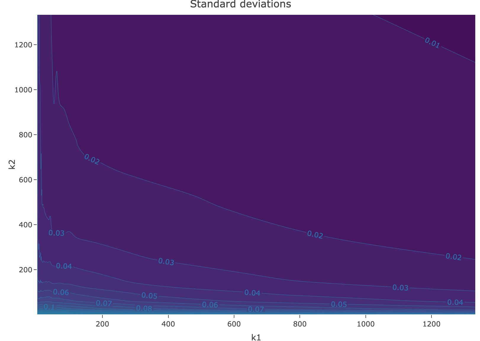
Figure 1. Heatmap with contour curves of standard deviations and mean squared errors for estimates of the extremal index $k1=k\mapsto\widehat{\theta}_{X}(k)$ in (4.24), using a Hill-type estimator $k2=k^{\prime}\mapsto\widehat{\alpha}(k^{\prime})$. We simulate $500$ samples $(X_{t})_{t=1,\dots,n}$ of an AR$(\varphi)$ model with absolute value student$(\alpha)$ noise for $n=12\,000$, $\varphi=0.5$, $\alpha=1$, such that $\theta_{X}=0.5$.

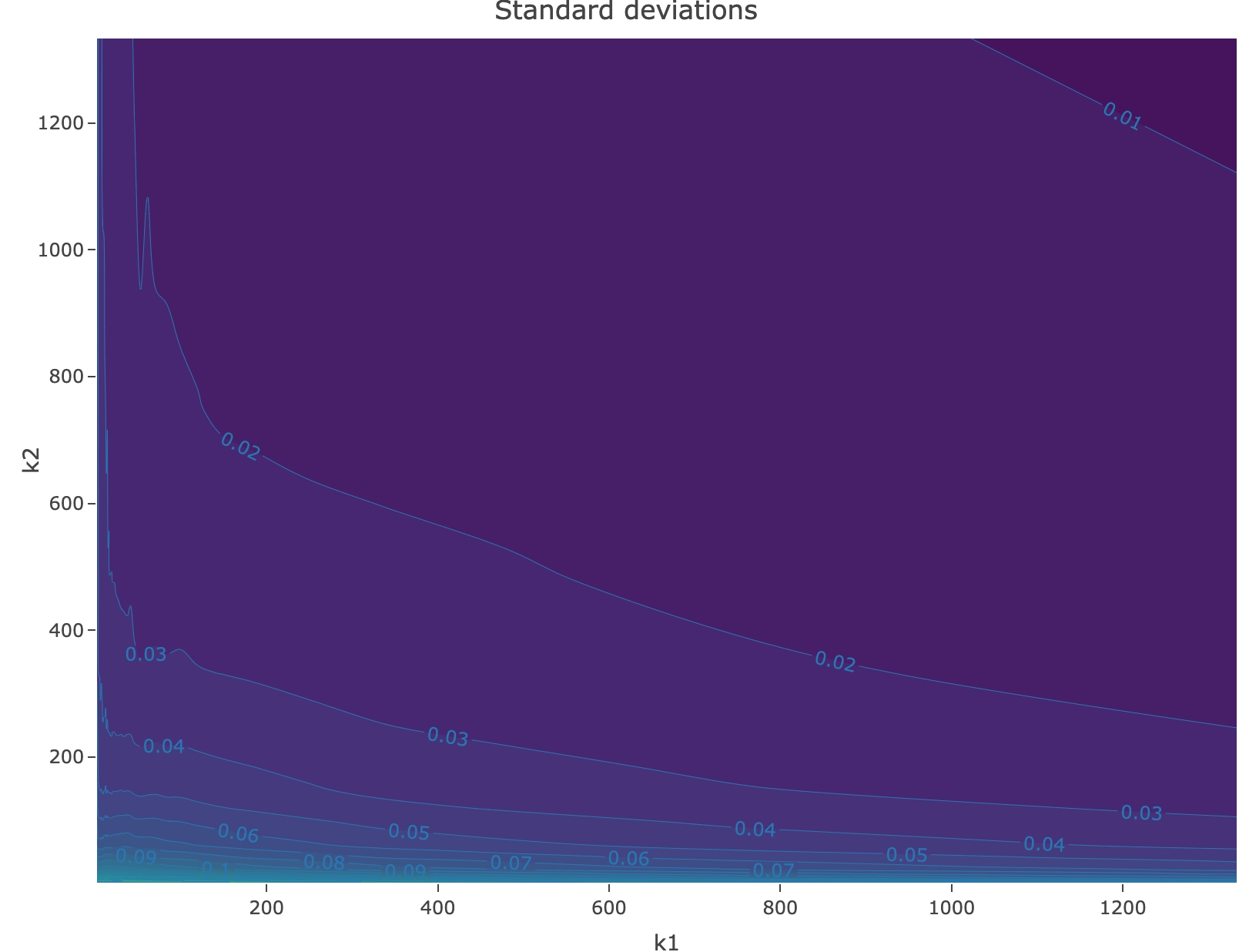
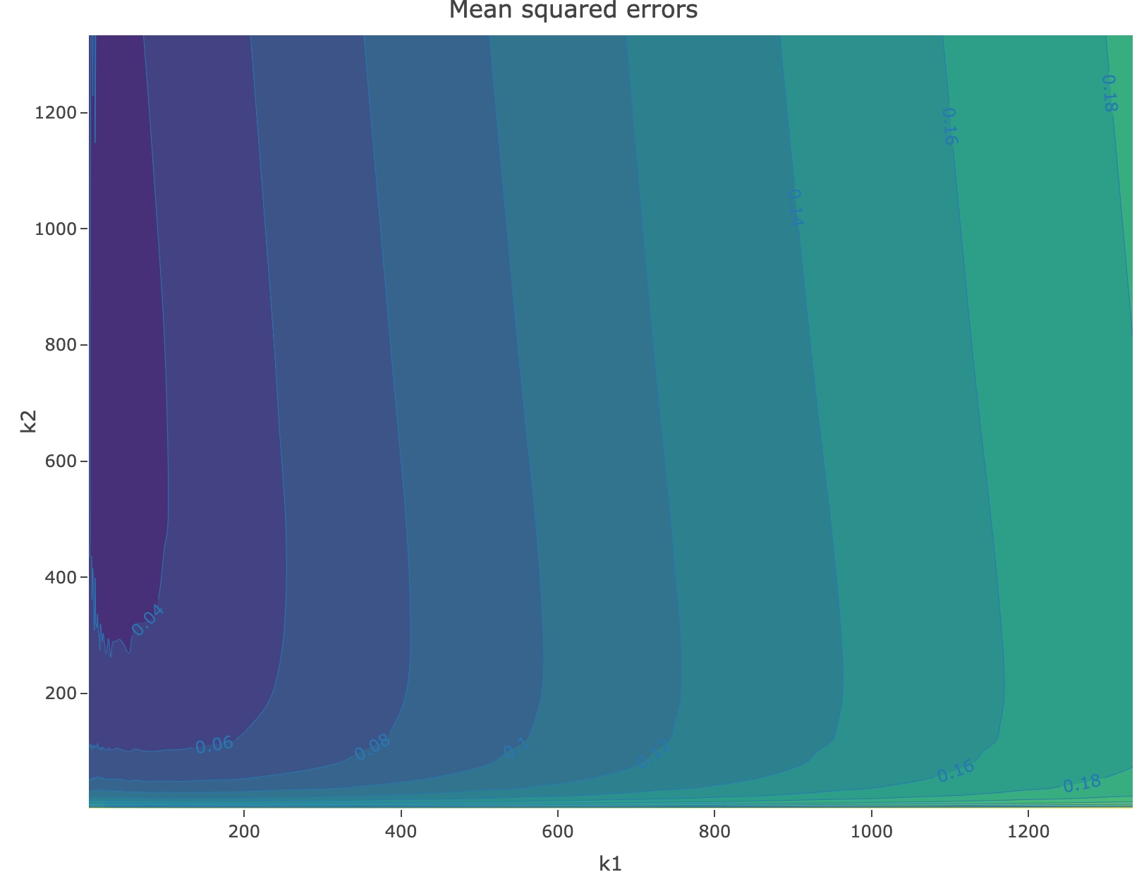
Figure 2. Heatmap with contour curves as in Figure 1. Here we simulate $500$ samples $(X_{t})_{t=1,\dots,n}$ of an AR$(\varphi)$ model with absolute value student$(\alpha)$ noise for $n=12\,000$, $\varphi=0.7$, $\alpha=1$, such that $\theta_{X}=0.3$.

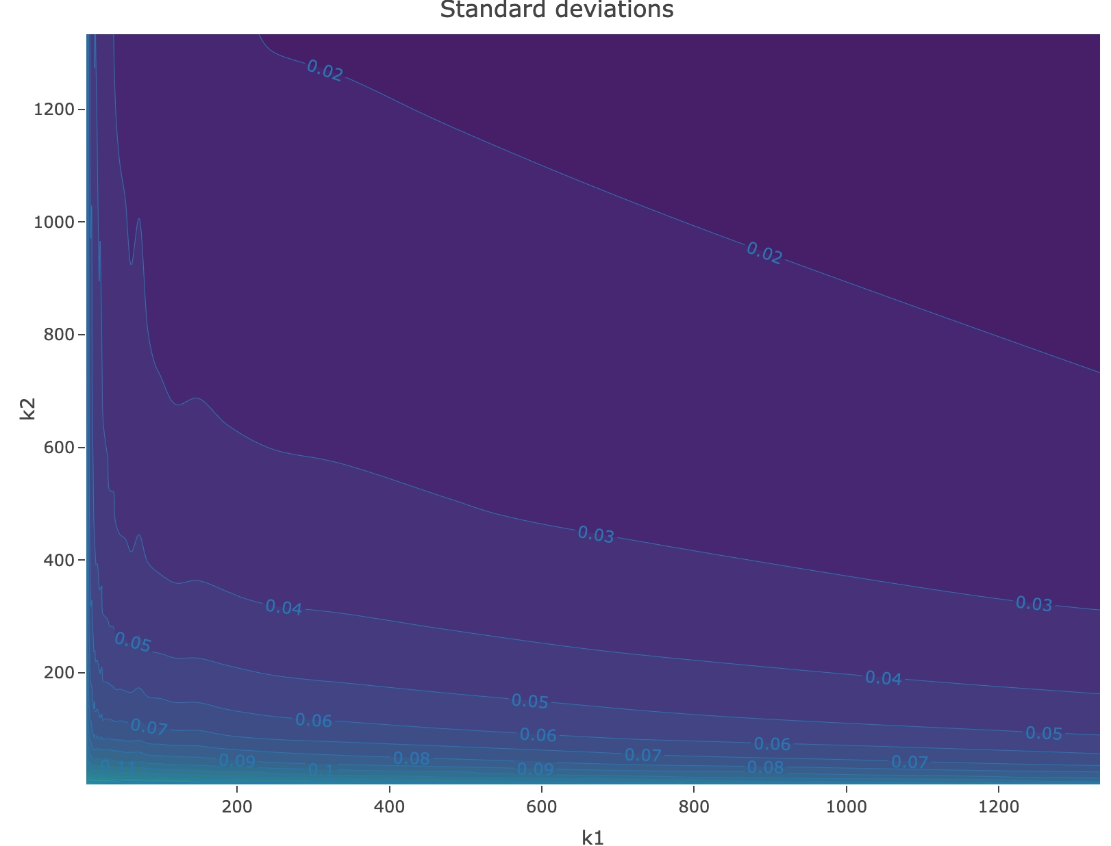
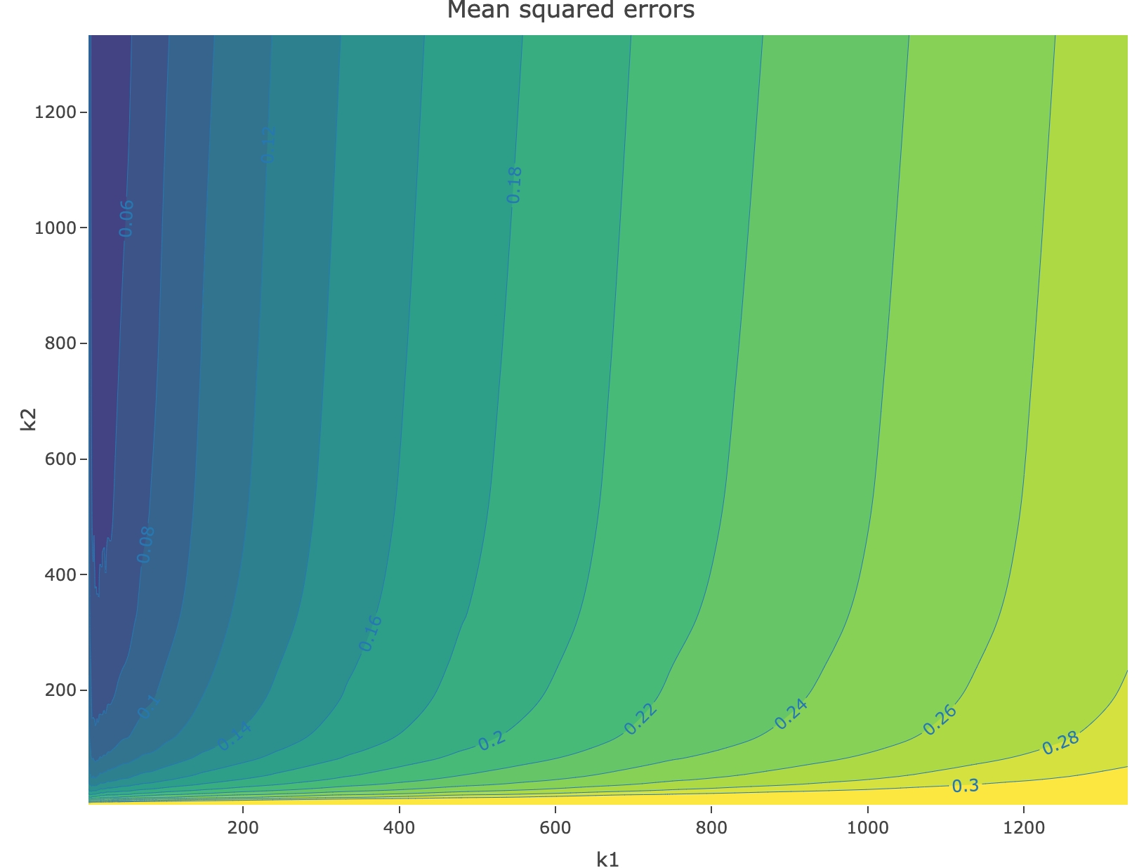
Figure 3. Heatmap with contour curves as in Figure 1. Here we simulate $500$ samples $(X_{t})_{t=1,\dots,n}$ of Example (6.1) for $n=12\,000$ such that $\theta_{X}\approx 0.2792$.

6.2. Cluster size probabilities

We reviewed in Section 4.3 how cluster sizes play a key role to model the serial behavior of exceedances. In this section, we implement the cluster size probabilites estimation procedure from Equation (4.32) in an example of a solution to the SRE under Kesten’s conditions.

Example 6.1.

Consider the non-negative univariate random variables $A$, $B$, defined by $\log A=N-0.5$, where $N$ denotes a standard Gaussian random variable, and $B$ is uniformly distributed in $[0,1]$. Let $(X_{t})$ be the solution to the SRE in (5.43). Then, $(X_{t})$ satisfies ${\bf RV}_{\alpha}$ with $\alpha=1$. If $(A_{j})$ is a sequence of iid random variables with generic element $A$, then

$$Q_{t} \stackrel{{\scriptstyle d}}{{=}} \Pi_{t}/\|(\Pi_{j})\|_{\alpha}\,,\qquad t\in\mathbb{Z}\,,$$

with

$$\Pi_{t} \stackrel{{\scriptstyle d}}{{=}} \begin{cases}A_{t}\cdots A_{1}&\text{ if }\quad t\geqslant 1,\\ A_{t}\cdots A_{-1}&\text{ if }\quad t\leqslant-1,\\ 1&\text{ if }\quad t=0\,.\end{cases}$$

This follows by Example 6.1 in [34], and Proposition 3.1 in [12]. Then, for $p>\alpha/2$, the $p$-cluster based estimators (4.24) (4.27), and (4.32) are asymptotically normally distributed.

Recall the cluster sizes $\pi_{1},$ $\pi_{2},$ $\dots$, defined in (4.31). We infer the cluster sizes of Example 6.1 using ${\alpha}$-cluster estimates. To illustrate Theorem 5.10, we run a Monte–Carlo simulation experiment based on $1\,000$ samples $(X_{t})_{t=1,\dots,n}$ of length $n=12\,000$ from Example 6.1. For each sampled trajectory, we obtain estimates $\widehat{\pi}_{1},\widehat{\pi}_{2},\dots$, letting $k=10$ and $b=38$ in (4.32). For the implementation we use Hill-based estimates of the tail-index $\widehat{\alpha}(k^{\prime})$ with $k^{\prime}=1\,000$. We also estimate the extremal index $\theta_{X}$ of the series from Equation (4.24). Theorem 5.10 yields, for $j\geqslant 0$,

(6.48) $${\rm Var}(\sqrt{k}\,(\widehat{\pi}_{j}-\pi^{\bf Q}_{j})) \to {\rm Var}(\pi_{j}^{\bf Q}({\bf Q})),\quad n\to\infty,$$

where $\pi_{j}^{\bf Q}$ are the cluster functional yielding the cluster sizes $\pi_{j}$ with the notation in (4.33). Notice that the asymptotic variance of our cluster sizes estimate is again a cluster statistic that we can infer. We compute an estimate of the asymptotic variance in (6.48) using cluster-based estimates, and compare this estimate with the empirical variance obtained from the Monte-Carlo simulation study. Figure 4 plots the profile of the limit Gaussian distribution where the asymptotic variance is computed in these two ways. As expected from Equation (6.48), the curves overlap, even if $k$ is small. In our simulation, a clear bias appears when we choose $k$ larger.

In the case of SRE equations, the cluster sizes were studied in detail in [26]. The authors proposed a method to approximate the true values when the tail-index $\alpha$, and the random variable $A$ are known. We approximate true values using Equation 3.5 in [26], and a Monte-Carlo study with $10\,000$ samples of length $500\,000$. The obtained values are pointed out in red in Figure 4. We see that this choice of $k$ yields estimates centered around the true value.

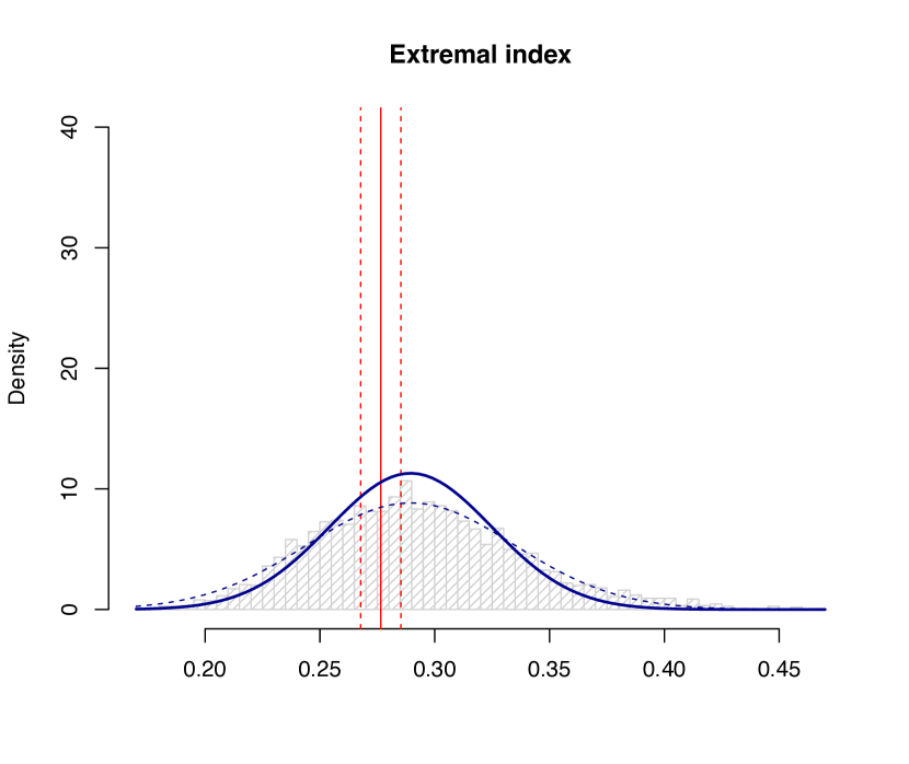
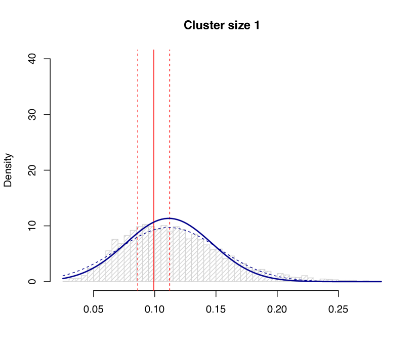
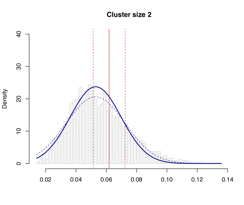
Figure 4. Histogram of estimates $\widehat{\theta}_{X}$ of the extremal index using (4.24), and the cluster size probability $\widehat{\pi}_{1}$, $\widehat{\pi}_{2}$, $\widehat{\pi}_{3}$, using (4.31). We simulate $1\,000$ samples $(X_{t})_{t=1,\dots,n}$ of Example 6.1 with $n=12\,000$. The Gaussian density curves are centered in the median of the estimators. Their variances are estimated by Monte-Carlo (dotted curve) or using the average of the cluster-based estimate of the asymptotic variance defined in (6.48) (solid curve). The red lines point to the Monte-Carlo approximation of the real values with standard deviation. These were computed using Equation 3.5 in [26], and a simulation study with $10\,000$ samples of length $500\,000$.

6.3. Conclusion

Our main theoretical result in Theorem 3.1 states asymptotic normality of $\alpha$-cluster-based disjoint blocks estimators $\widehat{f}^{\bf Q}_{\alpha}(k)$, based on $k$ extremal $\ell^{\widehat{\alpha}}$-blocks, where $\widehat{\alpha}$ is an estimate of the tail index of the series. The advantage of $\widehat{\alpha}$-cluster-based methods is that the choice of $k$ is robust to time dependencies; see [12]. Equation (3.23) characterizes their asymptotic variance in terms of a cluster statistic that we can also infer. We further show in Section 4 that many important indices in extremes can be written in terms of an $\alpha$-cluster statistic, e.g., the extremal index and cluster sizes. Section 5 verifies that our assumptions hold for numerous models like causal linear models and SRE solutions under Kesten’s conditions. For linear models, we obtain super-efficient estimators with null asymptotic variance for classical indices. In the examples we considered, our estimators have a small variance that can also be estimated. To illustrate the performance of our $\alpha$-cluster inference methodology, we run finite-sample simulations in Section 6. Our simulations support that replacing $\alpha$ by $\widehat{\alpha}(k^{\prime})$ as in Section 6.1 does not have a big impact on the asymptotic variance. This is because in practice $k$ needs to be chosen small to obtain unbiased estimates, whereas $k^{\prime}$ can be chosen larger. Then, even if we choose $k$ small, the uncertainty of our procedure is well quantified by plugging an estimate of the asymptotic variance in the Gaussian limit. Finally, a complete study of the tuning parameters $k,k^{\prime}$ requires a careful analysis of the bias conditions for blocks: ${\bf B}_{\alpha},{\bf B}$, as we pointed out in Remark 3.2, which we see as a road for future research.

Appendix A Proof of the main result

In the following proofs, we assume the conditions of Proposition 2.2 hold. In this setting, the time series $(\mathbf{X}_{t})$ admits a $p$-cluster ${\bf Q}^{(p)}\in\tilde{\ell}^{p}$ and (2.8), (2.9), hold for $(x_{n})$. For inference purposes, we fix the value of $p$. The sequence of block lengths $(b_{n})$, and we write $m_{n}=\lfloor n/b_{n}\rfloor$, such that $b_{n}\to\infty$, $m_{n}\to\infty$. We assume that the relation

(A.49) $$k\quad:=\quad k_{n}(p) = \;\big{\lfloor}m_{n}{\mathbb{P}}(\|\mathcal{B}_{1}\|_{p}>x_{b_{n}})\big{\rfloor}$$

(A.50) $$\sim n\,c(p){\mathbb{P}}(|\mathbf{X}_{1}|>x_{b_{n}}),\quad n\to\infty,$$

holds, where $c(p)\in(0,\infty)$ are as in (2.8). We can verify $m_{n}/k_{n}\to\infty$ using the relation $n\,{\mathbb{P}}(|\mathbf{X}_{1}|>x_{n})\to 0$. Moreover, it will be useful to consider the deterministic threshold estimator defined by

(A.51) $$\widetilde{f}^{{\bf Q}}_{{\alpha}}(u,q) := \frac{1}{k_{n}}\sum_{t=1}^{m_{n}}f_{\alpha}({\mathcal{B}}_{t}/(u\,x_{b_{n}}))\mathrm{1}\mathrm{1}(\|{\mathcal{B}}_{t}\|_{q}>(u\,x_{b_{n}}))\,,\quad u,q>0,$$

where $f_{{\alpha}}(p):\tilde{\ell}^{p}\to\mathbb{R}$ is a cluster functional that can depend on ${\alpha}$ in its expression. The sequences $(x_{n})$, $(b_{n})$, $(m_{n})$, $(k_{n})$, that we consider, defining the oracle estimator in (A.51), are the ones fixed above.

With this notation, Section A.1 states mixing rates for consistency of the blocks estimators in (1.3). Next, we show a uniform central limit theorem for the family of oracle estimators in (A.51). Section A.2 discusses the uniform entropy theory. The proof of Theorem 3.1 is deferred to Section A.3. In this section, we also compute the covariance structure of the family of oracle estimators in (A.51). The auxiliary propositions here stated are shown in Sections A.4 and A.5. The proofs of auxiliary lemmas are deferred to Appendix B.

A.1. Consistency of $p-$cluster based blocks estimators

The following Lemma is proven in Section B.2.

Lemma A.1.

Let $(\mathbf{X}_{t})$ be an $\mathbb{R}^{d}$-valued stationary time series satisfying $\bf RV_{\alpha}$. Let $p>0$, and assume the conditions of Proposition 2.2 hold such that $(\mathbf{X}_{t})$ admits a $p-$cluster process ${\bf Q}^{(p)}\in\tilde{\ell}^{p}$. Let $f=f(p)\in\mathcal{G}_{+}(\tilde{\ell}^{p})$ be a bounded Lipschitz continuous function. If there exists a sequence $(\ell_{n})$, satisfying $\ell_{n}\to\infty$, as $n\to\infty$, such that the $\beta-$mixing coefficients satisfy

$$\lim_{n\to\infty}m_{n}\beta_{\ell_{n}}/k_{n} = \lim_{n\to\infty}\ell_{n}/b_{n}\quad=\quad 0\,,$$

then the sequences $(x_{n})$ and $(b_{n})$ satisfy the relation

$$\big{|}{\mathbb{E}}\big{[}e^{-k^{-1}\sum_{t=1}^{m}f(x_{b}^{-1}{\mathcal{B}}_{t})\mathrm{1}\mathrm{1}(\|\mathcal{B}_{t}\|_{p}>x_{b_{n}})}\big{]}-{\mathbb{E}}\big{[}e^{-k^{-1}f(x_{b}^{-1}{\mathcal{B}}_{1})\mathrm{1}\mathrm{1}(\|\mathcal{B}_{1}\|_{p}>x_{b_{n}})}\big{]}^{m}\big{]}\big{|} \to 0,$$

(A.52) $$n \to \infty,$$

where $(k_{n})$ is chosen as in (A.50).

Corollary A.2.

Assume the conditions in Lemma A.1 hold. Consider a function $f\in\mathcal{G}_{+}(\tilde{\ell}^{p})$, not necessarily bounded, and assume ${\mathbb{E}}[f(Y{\bf Q}^{(p)})]<\infty$, and

(A.53) $$\frac{{\mathbb{E}}\big{[}\big{(}f(\mathbf{X}_{[1,n]}/x_{n})\big{)}^{1+\delta}\mathrm{1}\mathrm{1}(\|\mathbf{X}_{[1,n]}\|_{p}>x_{n})\big{]}}{{\mathbb{P}}(\|\mathbf{X}_{[1,n]}\|_{p}>x_{n})}<\infty.$$

Then, the ${p}$-cluster based blocks estimator in (1.3) satisfies

$$\widehat{f^{\bf Q}}(p) \xrightarrow[]{{\mathbb{P}}} f^{{\bf Q}}(p),\quad n\to\infty.$$

Proof of Corollary A.2.

If the function $f$ is bounded, then we can apply Theorem 4.1 in [12]. The mixing assumption therein is verified in Lemma A.1 stated above. Therefore, we deduce the consistency of the blocks estimators, and this concludes the proof. We now consider the case where $f$ is not necessarily bounded. Then, notice for all $\eta>0$,

(A.54) $${\mathbb{E}}[f(\mathcal{B}_{t}/x_{b_{n}})\mathrm{1}\mathrm{1}(\|\mathcal{B}_{t}\|_{p}>x_{b_{n}})]$$

$$= {\mathbb{E}}\big{[}\big{(}f(\mathcal{B}_{1}/x_{b_{n}})\mathrm{1}\mathrm{1}(\|\mathcal{B}_{1}\|_{p}>x_{b_{n}})\big{)}\mathrm{1}\mathrm{1}\big{(}f(\mathcal{B}_{1}/x_{b_{n}})\mathrm{1}\mathrm{1}(\|\mathcal{B}_{1}\|_{p}>x_{b_{n}})\leqslant\eta\big{)}\big{]}$$

$$+{\mathbb{E}}\big{[}\big{(}f(\mathcal{B}_{1}/x_{b_{n}})\mathrm{1}\mathrm{1}(\|\mathcal{B}_{1}\|_{p}>x_{b_{n}})\big{)}\mathrm{1}\mathrm{1}\big{(}f(\mathcal{B}_{1}/x_{b_{n}})\mathrm{1}\mathrm{1}(\|\mathcal{B}_{1}\|_{p}>x_{b_{n}})>\eta\big{)}\big{]}$$

$$= I+II.$$

The first term $I$ is a bounded function, and thus $I/({\mathbb{P}}(\|\mathcal{B}_{1}\|_{p}>x_{b_{n}}))$ converges to the $p-$cluster functional ${\mathbb{E}}[f(Y{\bf Q}^{(p)})\land\eta]$. Moreover, by monotone convergence, this term converges to $f^{\bf Q}(p)$, as $\eta\to\infty$. It remans to show

(A.55) $$\lim_{\eta\to\infty}\lim_{n\to\infty}\frac{II}{{\mathbb{P}}(\|\mathcal{B}_{1}\|_{p}>x_{b_{n}})} = 0.$$

Indeed,

$${\mathbb{E}}\big{[}\big{(}f(\mathcal{B}_{1}/x_{b_{n}})\mathrm{1}\mathrm{1}(\|\mathcal{B}_{1}\|_{p}>x_{b_{n}})\big{)}\mathrm{1}\mathrm{1}\big{(}f(\mathcal{B}_{1}/x_{b_{n}})\mathrm{1}\mathrm{1}(\|\mathcal{B}_{1}\|_{p}>x_{b_{n}})>\eta\big{)}\big{]}$$

$$\leqslant {\mathbb{E}}[\big{(}f(\mathcal{B}_{1}/x_{b_{n}})\mathrm{1}\mathrm{1}(\|\mathcal{B}_{1}\|_{p}>x_{b_{n}})\big{)}^{1+\delta}]^{\frac{1}{1+\delta}}{\mathbb{P}}\big{(}f(\mathcal{B}_{1}/x_{b_{n}})\mathrm{1}\mathrm{1}(\|\mathcal{B}_{1}\|_{p}>x_{b_{n}})>\eta\big{)}^{\frac{\delta}{1+\delta}}$$

$$\leqslant \eta^{-\delta}{\mathbb{E}}[\big{(}f(\mathcal{B}_{1}/x_{b_{n}})\mathrm{1}\mathrm{1}(\|\mathcal{B}_{1}\|_{p}>x_{b_{n}})\big{)}^{1+\delta}].$$

Finally, provided (A.53) holds, we see (A.55) holds, and this concludes the proof. ∎

A.2. Uniform entropy theory

Theorem 3.1 states asymptotic normality of $\ell^{\widehat{\alpha}}$-blocks estimators in (1.3). Our proof considers a family of oracle estimators indexed by $q$, for $q$ in a neighborhood of ${\alpha}$, and relies on Lemma A.3 below showing this family has low complexity in terms of entropy numbers; cf [53]. We review the classical results of the theory of Vapnik-Cervonenkis below to measure the complexity of classes of functions.

The dimension of a VC-class of sets $\mathcal{V}$ is the number $d$ such that for every set containing $d$ elements, we can find a subset that is not picked out by the class $\mathcal{V}$. A VC-class of functions $\mathcal{F}$ is such that the collections of all the subgraphs $\{({\bf x},u)\in\mathbb{R}^{d}\times(0,\infty):\phi({\bf x})>u\}$ of functions $\phi\in\mathcal{F}$ is a VC-class. The entropy number of a VC-class has a polynomial expression on the VC-dimension (see Theorem 2.6.7. in [53]). Moreover, given a VC-class of functions $\mathcal{F}$, the VC-Hull of $\mathcal{F}$ is the collection of functions $\mathcal{G}$ such that for every $g\in\mathcal{G}$ there exists a symmetric convex combination $f_{m}=\sum_{i=1}^{m}\alpha_{i}f_{i}$, with $\sum_{i=1}^{m}|\alpha_{i}|\leqslant 1$, $f_{i}\in\mathcal{F}$, such that $g$ is the pointwise limit of the sequence $(f_{m})_{m\in\mathbb{N}}$. Moreover, by Corollary 2.6.12 in [53] the entropy number of a VC-hull also has a polynomial expression on the VC-dimension of the underlying VC-class.

Moreover, it is often easier to check that the class $\mathcal{F}$ is a VC-major of functions $\mathcal{F}$, i.e., that $\{{\bf x}\in\mathbb{R}^{d}:\phi({\bf x})>u\}$ is a VC-class. We can construct new VC-major classes using classical operations: addition, products. Moreover, if $\mathcal{F}$ is a VC-major, then the class of function $h\circ\phi$, with $h$ ranging over the monotone functions $h:\mathbb{R}\to\mathbb{R}$, with $\phi\in\mathcal{F}$, is a VC-major. This is Lemma 2.6.19 in [53]. One example are functions ${\bf x}\mapsto f({\bf x}/u)\mathrm{1}\mathrm{1}(\phi({\bf x})>u)$, where $u\mapsto f({\bf x}/u)$ is a non-increasing function. Moreover, a bounded VC-major class satisfies the uniform entropy condition by Lemma 2.6.13 in [53].

In particular, we show that $\ell^{q}$-norms form a VC-major. This is the purpose of the next Lemma whose proof is postponed to Section B.1.

Lemma A.3.

Consider the class containing all sets of the form $\{({\bf x}_{t})\in(\mathbb{R}^{d})^{\mathbb{Z}}\cap\ell^{q_{0}}:\|{\bf x}_{t}\|_{q}>u\},$ where $q\in(q_{0},q_{0}^{\prime})$, and $u>0$. Then, this is a VC-class of dimension 3.

A.3. Proof of Theorem 3.1

Let $\mathcal{F}\subseteq\mathcal{G}_{+}(\tilde{\ell}^{p})$ be the set including the functions: $({\bf x}_{t})\mapsto f_{\alpha}({\bf x}_{t})$, $({\bf x}_{t})\mapsto 1$, $({\bf x}_{t})\mapsto h({\bf x}_{t})$ and $({\bf x}_{t})\mapsto e({\bf x}_{t})$ as in (3.17), (2.14), (2.15). Recall the deterministic threshold estimators in (A.51), and define, for $\epsilon>0$, the family

(A.56) $$\mathcal{T} := \{\widetilde{g^{{\bf Q}}}(u,q)\}_{\{{g(\cdot/u)}:\;g\in\mathcal{F},u\in[1-\epsilon,1+\epsilon],q\in[{\alpha}-\epsilon,{\alpha}+\epsilon]\}}.$$

Note this family is indexed by four functions $f_{\alpha},1,h,e,$ and the values of $u,q$. Here

(A.57) $$(u,q) \mapsto \widetilde{g^{\bf Q}}(u,q),\quad g\in\mathcal{F},$$

is a stochastic process taking values in $\mathbb{D}([1-\epsilon,1+\epsilon])\times\mathbb{D}([{\alpha}-\epsilon,{\alpha}+\epsilon])$ endowed with the product $J_{1}$-topology of the metric space of càdlàg functions.

To show a central limit theorem on this family note we need to control the complexity of the family $\mathcal{T}$ in (A.56), together with its covariance structure. We use for now the working assumption ${\bf C}^{\prime}$ below, and show uniform asymptotic normality of the family $\mathcal{T}$ in Proposition A.4. We come back to showing ${\bf C}^{\prime}$ in Proposition A.5.

We focus on showing the asymptotic result for the blocks estimator implemented with $p=\widehat{\alpha}$. The general result on $p$-cluster inference, for $p>0$, follows the same lines of this proof by fixing $q=p$ during the proof, instead of considering $q$ in a neighbourhood of ${\alpha}$.
(C^′): Assume the asymptotic normality of the finite-dimensional parts of (A.56), i.e.,

(A.58) $$\sqrt{k}\big{(}\widetilde{g^{{\bf Q}}}(u,q)-c(q)u^{-\alpha}\,g^{{\bf Q}}(q)\big{)} \xrightarrow[]{fi.di.} \mathbb{G}_{q}(g(\cdot/u)),\quad\widetilde{g^{{\bf Q}}}(u,q)\in\mathcal{T},$$

as $n\to\infty$, where $g^{{\bf Q}}(q)$ is a $q-$cluster statistic given by

$$g^{{\bf Q}}(q) = {\mathbb{E}}[g(Y{\bf Q}^{(q)})],$$

and the limit is a centered Gaussian process satisfying

(A.59) $${\rm Cov}\big{(}\mathbb{G}_{q}(g(\cdot/u)),\mathbb{G}_{q^{\prime}}(h(\cdot/v))\big{)}$$

$$= c(q)u^{-{\alpha}}\,{\mathbb{E}}[g(Y{\bf Q}^{(q)})h(Y{\bf Q}^{(q)}u/v)\mathrm{1}\mathrm{1}(\|Y{\bf Q}^{(q)}u/v\|_{q^{\prime}}>1)],$$

for $u,v\in[1-\epsilon,1+\epsilon]$, $q,q^{\prime}\in[{\alpha}-\epsilon,{\alpha}+\epsilon]$, and $g,h\in\mathcal{F}$, such that ${\bf Q}^{(q)}\in\tilde{\ell}^{q}$, is the $q$-cluster process of the series. To simplify notation, we write in the remaining of the article

$$g^{{\bf Q}} := g^{{\bf Q}}({\alpha}).$$

The next Proposition shows the uniform central limit theorem on the family $\mathcal{T}$ holds, and its proof is deferred to Section A.4.

Proposition A.4.

Let $(\mathbf{X}_{t})$ be a stationary time series satisfying $\bf RV_{\alpha}$. Assume the conditions of Theorem 3.1 hold, and assume ${\bf C}^{\prime}$ holds. Then,

$$\sqrt{k}\big{(}\widehat{f_{\widehat{\alpha}}^{{\bf Q}}}(\widehat{\alpha})-f^{\bf Q}_{{\alpha}}({\alpha})\big{)}$$

$$\xrightarrow[]{d} \mathcal{N}(0,{\rm Var}(f_{{\alpha}}(Y{\bf Q}^{({\alpha})}))+\kappa\big{(}\tfrac{\partial f_{p}}{\partial p}|^{\bf Q}_{{\alpha}}\big{)}^{2}\alpha^{2}\sigma_{\alpha}^{2}\,)\,,\quad n\to\infty,$$

with $\sigma_{\alpha}^{2}={\mathbb{E}}[({\alpha}h(Y{\bf Q}^{({\alpha})})-e(Y{\bf Q}^{({\alpha})}))^{2}]$ such that $\sqrt{k^{\prime}}\big{(}\widehat{\alpha}-{\alpha}\big{)}\xrightarrow[]{d}\mathcal{N}(0,\sigma_{\alpha}^{2}),$ and $\sqrt{k/k^{\prime}}\to\kappa$, with $\kappa\geqslant 0$, and $Y$ is independent of ${\bf Q}^{({\alpha})}$, and ${\mathbb{P}}(Y>y)=y^{-\alpha}$, for $y>1$. Moreover, uniform asymptotic normality of the family $\mathcal{T}$ holds.

To complete the proof of Theorem 3.1, we must verify ${\bf C^{\prime}}$ holds under the mixing condition ${\bf MX_{\beta}}$. For this purpose, we require the next lemma whose proof is postponed to Section A.5.

Proposition A.5.

Let $(\mathbf{X}_{t})$ be an $\mathbb{R}^{d}$-valued stationary time series satisfying $\bf RV_{\alpha}$. Assume the conditions of Proposition 2.2 hold such that $(\mathbf{X}_{t})$ admits an ${\alpha}-$cluster process ${\bf Q}\in\tilde{\ell}^{\alpha}$. Consider $g,h:\tilde{\ell}^{\alpha}\to\mathbb{R}$ such that ${\bf L}$ holds. Assume ${\bf B}_{\alpha}(k),{\bf B}(k^{\prime})$, and condition ${\bf MX_{\beta}}$ hold. Then,

$$k\,{\rm Cov}\big{(}\widetilde{g^{\bf Q}}(u,q)),\widetilde{h^{\bf Q}}(v,q^{\prime})\big{)} \xrightarrow[]{} {\rm Cov}\big{(}\mathbb{G}_{q}(g(\cdot/u)),\mathbb{G}_{q^{\prime}}(h(\cdot/v))\big{)},$$

as $n\to\infty$.

Relying on Proposition A.5 and Proposition A.4 we can now write the proof of Theorem 3.1.

Proof of Theorem 3.1.

Consider the assumptions in Proposition A.5, and assume condition ${\bf MX_{\beta}}$ holds. Consider a function $f_{\alpha}:\tilde{\ell}^{\alpha}\to\mathbb{R}$ satisfying $\bf L$. Recall the family $\mathcal{T}$ in (A.56). Asymptotic normality of the finite-dimensional parts of $\mathcal{T}$ hold by Proposition A.5. Indeed, by the Wold device it is enough to check that every linear combination of deterministic threshold estimators in (A.51) is asymptotically normal with Gaussian limit $\mathbb{G}$ and covariance structure as in (A.59). This holds since linear combinations of estimators in (A.51) are again a deterministic threshold estimator as in (A.51). Finally, this shows that ${\bf C}^{\prime}$ holds. Thus, we can apply Proposition A.4 and this concludes the proof. ∎

A.4. Proof of Proposition A.4

Recall the set $\mathcal{F}\subseteq\mathcal{G}_{+}(\tilde{\ell}^{p})$ of functions: $({\bf x}_{t})\mapsto f_{\alpha}({\bf x}_{t})$, $({\bf x}_{t})\mapsto 1$, $({\bf x}_{t})\mapsto h({\bf x}_{t})$ and $({\bf x}_{t})\mapsto e({\bf x}_{t})$ (see (3.17), (2.14), (2.15)), and the family $\mathcal{T}$ in (A.56).

We separate the proof of Proposition A.4 in two steps. In Section A.4.1 we show (3.23) holds assuming the uniform asymptotic normality of the Gaussian family indexed by $\mathcal{T}$. Then, in Section A.4.2 we show the uniform central limit theorem holds. Then, for now, assume

$$\sqrt{k}(\widetilde{g^{\bf Q}}(u,q)-c(q)u^{-\alpha}g^{\bf Q}(q)) \xrightarrow[]{d} \mathbb{G}_{q}(g(\cdot/u)),\quad\widetilde{g^{\bf Q}}(u,q)\in\mathcal{T},$$

as $n\to\infty$, holds uniformly, and the limit is a Gaussian process with covariance as in (A.59), for $g,h\in\mathcal{F}$, and $u,v\in[1-\epsilon,1+\epsilon]$.

The following auxiliary lemmas will be useful, and their proofs are postponed to Appendix B. The following Lemma is shown in Section B.3.

Lemma A.6 (Asymptotics of the Hill estimator $1/\widehat{\alpha}$).

Recall the Hill estimator $1/\widehat{\alpha}$ in (2.13), and the functionals $h,e$, in (2.14) and (2.15). Assume

$$(\widetilde{g^{\bf Q}}(u))_{u\in[1-\epsilon,1+\epsilon],g\in\{h,e\}} \xrightarrow[]{d} \mathbb{G}_{\alpha}(g(\cdot/u)),\quad n\to\infty,$$

uniformly where the limit on the right-hand side is a Gaussian process in (A.59), here indexed by $u,g$. Then,

(A.60) $$\sqrt{k^{\prime}}\,(\widehat{{\alpha}}^{n}-{\alpha}) \xrightarrow[]{d} {\alpha}\mathbb{G}_{{\alpha}}({\alpha}h(\cdot/1)-e(\cdot/1)).$$

The next lemma is shown in Section B.4

Lemma A.7 (Continuity of the function $q\mapsto c(q)$).

Assume condition $\bf M$ holds, then the function $q\mapsto c(q)$ is continuous for $q\in[\alpha-\epsilon,\alpha+\epsilon]$. Moreover, under the assumptions of Lemma A.6,

$$\sqrt{k^{\prime}}(1-c(\widehat{\alpha})) \xrightarrow[]{d} {\alpha}\psi_{\alpha}^{{\bf Q}}\,\mathbb{G}_{\alpha}(h(\cdot/1)-\alpha^{-1}e(\cdot/1)),\quad n\to\infty,$$

where $\psi_{\alpha}^{{\bf Q}}={\mathbb{E}}[\psi_{\alpha}({\bf Q}^{({\alpha})})]$, with $\psi_{\alpha}({\bf x}_{t})=\mbox{$\sum_{j\in\mathbb{Z}}$}|{\bf x}_{j}|^{\alpha}\log\big{(}1/{|{\bf x}_{j}|}\big{)}$.

Lemma A.8 below states that we can replace in the oracle estimator the values of $x_{b_{n}}$ by the random threshold $\|\mathcal{B}_{1}\|_{\hat{\alpha},(k)}$. We defer the Proof of this Lemma to Section B.5.

Lemma A.8 (Asymptotics of the random threshold $\|\mathcal{B}_{1}\|_{\widehat{\alpha},(k)}$).

Under the assumptions of Theorem 3.1,

$$\sqrt{k}\,\big{(}\,\widehat{f_{{\alpha}}^{\bf Q}}(\widehat{\alpha})-f^{\bf Q}_{\alpha}\,\big{)} \xrightarrow[]{d} f_{\alpha}^{\bf Q}\mathbb{G}_{\alpha}(\,f_{\alpha}(\cdot/1)/f_{\alpha}^{\bf Q}-1(\cdot/1)\,),$$

as $n\to\infty$, where ${\alpha}$ is fixed here.

A.4.1. Variance calculations

We now focus on establishing the asymptotic variance in (3.23). Recall that when $f$ depends on ${\alpha}$, i.e., $f=f_{\alpha}$, we impose a smoothness assumption ${\bf S}$ on the function $q\mapsto f_{q}$. More precisely, we assume

$$f_{q}({\bf x}) = f_{\alpha}({\bf x})+(q-\alpha)f^{\prime}_{\alpha}({\bf x})+(q-{\alpha})^{2}R_{\alpha}({\bf x}),$$

where $f^{\prime}_{\alpha}$ is the derivative of $f_{a}$ with respect to $a$, i.e., $f^{\prime}_{\alpha}=\tfrac{\partial f_{q}}{\partial q}\big{|}_{q={\alpha}}$, and

$$R_{\alpha}({\bf x}) \leqslant \max_{q\in({\alpha}-\epsilon,{\alpha}+\epsilon)}\Big{|}\frac{\partial^{2}f_{q}}{\partial q^{2}}({\bf x})\Big{|}.$$

Recall we denote

$$\widehat{f}_{q}^{\bf Q}(\widehat{\alpha}) = \frac{1}{k}\sum_{t=1}^{m_{n}}f_{q}({\mathcal{B}}_{t}/\|{\mathcal{B}}\|_{\widehat{\alpha},(k+1)})\mathrm{1}\mathrm{1}(\|{\mathcal{B}}_{t}\|_{\widehat{\alpha}}>\,\|{\mathcal{B}}\|_{\widehat{\alpha},(k+1)}),$$

By an application of Lemma A.6 and Lemma A.8 we see, that if $f^{\prime}_{\alpha}$, $R_{\alpha}$ admit consistent $\ell^{\alpha}-$cluster estimates, then

$$\sqrt{k}\,\big{(}\,\widehat{f}^{\bf Q}_{\widehat{\alpha}}(\widehat{\alpha})-f^{\bf Q}_{\alpha}\,\big{)}$$

$$= \sqrt{k}\big{(}\,\widehat{f}_{{\alpha}}^{\bf Q}(\widehat{\alpha})-f_{\alpha}^{\bf Q})+\frac{\sqrt{k}}{\sqrt{k^{\prime}}}\sqrt{k^{\prime}}\big{(}\alpha-\widehat{\alpha}\big{)}\widehat{f_{\alpha}^{\prime}}^{\bf Q}(\widehat{\alpha})$$

$$+\frac{\sqrt{k}}{\sqrt{k^{\prime}}}\sqrt{k^{\prime}}\big{(}\alpha-\widehat{\alpha}\big{)}^{2}\widehat{R}_{\alpha}^{\bf Q}(\widehat{\alpha})$$

$$\xrightarrow[]{d} \mathbb{G}_{\alpha}\big{(}(f_{\alpha}(\cdot/1)-f_{\alpha}^{\bf Q}1(\cdot/1))+f_{\alpha}^{\prime{\bf Q}}c_{h}\,{\alpha}^{2}({\alpha}h(\cdot/1)-e(\cdot/1))\big{)},$$

where $k^{\prime}$ is the tuning parameter for the Hill estimator whereas $k$ is used to tune the extremal cluster estimator such that$\sqrt{k/k^{\prime}}\to\kappa\geqslant 0$. We recognize here the variance term in (3.23).

A.4.2. Uniform central limit theorem

Fix $g\in\mathcal{F}$. In this section, we show

$$\sqrt{k}(\widetilde{g^{\bf Q}}(u,q)-c(q)u^{-{\alpha}}g^{{\bf Q}}(q)) \xrightarrow[]{d} \mathbb{G}_{q}(g(\cdot/u))$$

uniformly on $q$ and $u$, as $n\to\infty$ where $\mathbb{G}$ is the Gaussian limit defined by (A.59). We can replace the expectation of $\widetilde{g^{{\bf Q}}}(u,q)$ directly by the limit $c(q)u^{-{\alpha}}g^{{\bf Q}}(q)$ thanks to the bias assumptions $\bf B_{\alpha}$ and $\bf B$. Assuming ${\bf C}^{\prime}$ we know convergence of the finite-dimensional parts of $\mathcal{T}$ holds as in (A.58). Then, it remains to check the asymptotic equicontinuity of the family of empirical processes indexed by $\mathcal{T}$. Actually, since the family $\mathcal{F}$ contains only a finite number of functions, it is enough to check separately equicontinuity on the family

(A.61) $$\{\sqrt{k}(\widetilde{g^{\bf Q}}(u,q)-c(q)u^{-{\alpha}}g^{{\bf Q}}(q))\}_{u\in[u_{0},s_{0}],q\in[q_{0},q^{\prime}_{0}]},$$

for each $g\in\mathcal{F}$, with $u_{0}=1-\epsilon<1<1+\epsilon=s_{0}$ and $q_{0}={\alpha}-\epsilon<{\alpha}<{\alpha}+\epsilon=q^{\prime}_{0}$. Fixing $g$, we obtain a class of functions indexed by $[u_{0},s_{0}]\times[q_{0},q^{\prime}_{0}]$, and we can equip it with the a semi-metric $d(\cdot,\cdot)$ given by

(A.62) $$d\,((u,q),(v,q^{\prime})) = |u-v|+|q-q^{\prime}|,$$

for $v,u,q,q^{\prime}>0$. Note that $(\widetilde{g^{\bf Q}}(u,q))_{u\in[u_{0},s_{0}],q\in[q_{0},q^{\prime}_{0}]}$ is separable and totally bounded family for this semi-metric.

To see this, we consider a coupling argument. We design recursively coupled blocks $(\mathcal{B}_{t}^{*})_{1\leqslant t\leqslant m_{n}}$ as follows: for every $t=1,\ldots,m_{n}$, we apply the maximal coupling Theorem 5.1 in [46] to create the block $(\mathcal{B}_{t}^{*})$ independent of the past blocks $(\mathcal{B}_{j},\mathcal{B}_{j}^{*})_{j<t}$, distributed as $\mathcal{B}_{1}$, and such that

(A.63) $${\mathbb{P}}\big{(}\mathcal{B}_{t,\ell}\not=\mathcal{B}^{*}_{t,\ell}\big{)}=\beta_{\ell_{n}},\quad t=1,2,\dots,m_{n}\,,$$

with the notation $\mathcal{B}_{t,\ell}=\mathbf{X}_{[tb+\ell,(t+1)b]}$. Then, notice

(A.65) $${\mathbb{P}}\Big{(}\sup_{\begin{subarray}{c}u,v\in[u_{0},s_{0}]\\ q,q^{\prime}\in[q_{0},q^{\prime}_{0}]\\ d((u,q),(v,q^{\prime}))<\delta\end{subarray}}\sqrt{k_{n}}\,|\widetilde{g^{\bf Q}}(u,q)-\widetilde{g^{\bf Q}}(v,q^{\prime})|>\delta\Big{)}$$

$$\leqslant {\mathbb{P}}\Big{(}\sup_{\begin{subarray}{c}u,v,q,q^{\prime}\\ d((u,q),(v,q^{\prime}))<\delta\end{subarray}}\sqrt{k_{n}}\,|\widetilde{g_{,*}^{\bf Q}}(u,q)-\widetilde{g_{,*}^{\bf Q}}(v,q^{\prime})|>\delta/2\Big{)}$$

$$+2{\mathbb{P}}\Big{(}\sup_{u,q}\sqrt{k_{n}}\,|\widetilde{g^{\bf Q}}(u,q)-\widetilde{g_{,*}^{\bf Q}}(u,q)|>\delta/4\Big{)}\,,$$

where for the first upper-bound, we have simplified notation, but we keep in mind that $u,v\in[u_{0},s_{0}],$ and $q,q^{\prime}\in[q_{0},q_{0}^{\prime}]$, and we denote

$$\widetilde{g_{,*}^{\bf Q}}(u,q) = \frac{1}{k_{n}}\sum_{t=1}^{m_{n}}g(\mathcal{B}^{*}_{t}/(u\,x_{b}))\mathrm{1}\mathrm{1}(\|\mathcal{B}^{*}_{t}\|_{q}>(u\,x_{b}))\,.$$

We focus now on the second term (A.65) of the previous bound. We apply Markov of order $2$, which yields

$${\mathbb{P}}\Big{(}\sup_{u,q}\sqrt{k_{n}}\,|\widetilde{g^{\bf Q}}(u,q)-\widetilde{g_{,*}^{\bf Q}}(u,q)|>\delta/4\Big{)}$$

$$\leqslant \dfrac{16}{k_{n}\delta^{2}}{\mathbb{E}}\Big{[}\sup_{u,q}\Big{(}\sum_{t=1}^{m_{n}}(g(\mathcal{B}_{t}/(u\,x_{b}))\mathrm{1}\mathrm{1}(\|\mathcal{B}_{t}\|_{q}>(u\,x_{b}))$$

$$-g(\mathcal{B}^{*}_{t}/(u\,x_{b}))\mathrm{1}\mathrm{1}(\|\mathcal{B}^{*}_{t}\|_{q}>(u\,x_{b})))\Big{)}^{2}\Big{]}\,.$$

We develop the square and obtain a diagonal term

$$\dfrac{m_{n}}{k_{n}}{\mathbb{E}}\Big{[}\sup_{u,q}(g(\mathcal{B}_{1}/(u\,x_{b}))\mathrm{1}\mathrm{1}(\|\mathcal{B}_{1}\|_{q}>(u\,x_{b}))-g(\mathcal{B}^{*}_{1}/(u\,x_{b}))\mathrm{1}\mathrm{1}(\|\mathcal{B}^{*}_{1}\|_{q}>(u\,x_{b})))^{2}\Big{]}.$$

Note that, denoting $G$ the envelop function,

$$G(\mathcal{B}_{1}/x_{b}) := \sup_{u\in[u_{0},s_{0}],q\in[q_{0},q_{0}^{\prime}]}g(\mathcal{B}_{1}/(ux_{b}))\mathrm{1}\mathrm{1}(\|\mathcal{B}_{1}\|_{q}>(ux_{b}))$$

$$= g(\mathcal{B}_{1}/(u_{0}x_{b}))\mathrm{1}\mathrm{1}(\|\mathcal{B}_{1}\|_{q_{0}}>(u_{0}x_{b})).$$

Then, by a similar argument as in the proof of Lemma A.9, we can assume the function $g$ is non-negative bounded and thus we can truncate $g$ to $g_{\varepsilon}$. This means we now need to control

$$\dfrac{m_{n}}{k_{n}}{\mathbb{E}}\Big{[}\sup_{u,q}(g_{\varepsilon}(\mathcal{B}_{1}/(u\,x_{b}))\mathrm{1}\mathrm{1}(\|\mathcal{B}_{1}\|_{q}>(u\,x_{b}))$$

$$-g_{\varepsilon}(\mathcal{B}^{*}_{1}/(u\,x_{b}))\mathrm{1}\mathrm{1}(\|\mathcal{B}^{*}_{1}\|_{q}>(u\,x_{b})))^{2}\Big{]}$$

$$= \dfrac{m_{n}}{k_{n}}{\mathbb{E}}\Big{[}\sup_{u,q}(g_{\varepsilon}(\mathcal{B}_{1,\ell}/(u\,x_{b}))\mathrm{1}\mathrm{1}(\|\mathcal{B}_{1,\ell}\|_{q}>(u\,x_{b}))$$

$$\qquad\qquad-g_{\varepsilon}(\mathcal{B}^{*}_{1,\ell}/(u\,x_{b}))\mathrm{1}\mathrm{1}(\|\mathcal{B}^{*}_{1,\ell}\|_{q}>(u\,x_{b})))^{2}\Big{]}+o(1)$$

$$= \dfrac{m_{n}}{k_{n}}E[G_{\epsilon}(\mathcal{B}_{1,\ell}/x_{b})^{2}\mathrm{1}\mathrm{1}(\mathcal{B}_{1,\ell}\neq\mathcal{B}_{1,\ell}^{*})]+o(1),$$

here the second to-last relation holds with the notation $\mathcal{B}_{1,\ell}=\mathbf{X}_{[\ell,b]}$, again relying on the calculation of Lemma A.9. In the last equation, $G_{\epsilon}$ is again the envelope function in (A.4.2), but for the function $g_{\epsilon}$. The gap of length $\ell$ allows to use the maximal coupling theorem, notably, Equation (A.63). Thus

$${\mathbb{E}}[G_{\varepsilon}(\mathcal{B}_{1}/x_{b})^{2}\mathrm{1}\mathrm{1}(\mathcal{B}_{1,\ell}\neq\mathcal{B}_{1,\ell}^{*})]$$

$$\leqslant \dfrac{m_{n}}{k_{n}}{\mathbb{E}}[G_{\varepsilon}(\mathcal{B}_{1}/x_{b})^{2+\delta}]^{2/(2+\delta)}{\mathbb{P}}(\mathcal{B}_{1,\ell}\neq\mathcal{B}_{1,\ell}^{*})^{\delta/(2+\delta)}$$

$$\leqslant \dfrac{m_{n}}{k_{n}}{\mathbb{P}}(\|\mathcal{B}_{1}\|>x_{b_{n}})^{2/(2+\delta)}\beta_{\ell}^{\delta/(2+\delta)}\sim(m_{n}\beta_{\ell}/k_{n})^{\delta/(2+\delta)},$$

if $G$ satisfies the assumption L.

We now focus on the crossed terms in the development of the square. Note we assume without loss of generality that $g$ is non-negative by considering separately the positive and negative parts. Then note that for $j\not=t$,

$${\mathbb{E}}\Big{[}\sup_{u,q}\Big{(}g(\mathcal{B}_{t}/(ux_{b}))\mathrm{1}\mathrm{1}(\|\mathcal{B}_{t}\|_{q}>(ux_{b}))-g(\mathcal{B}^{*}_{t}/(ux_{b}))\mathrm{1}\mathrm{1}(\|\mathcal{B}^{*}_{t}\|_{q}>(ux_{b}))\Big{)}$$

$$\times\Big{(}g(\mathcal{B}_{j}/(ux_{b}))\mathrm{1}\mathrm{1}(\|\mathcal{B}_{j}\|_{q}>(ux_{b}))-g(\mathcal{B}^{*}_{j}/(ux_{b}))\mathrm{1}\mathrm{1}(\|\mathcal{B}^{*}_{j}\|_{q}>(ux_{b}))\Big{)}\Big{]}$$

$$\leqslant {\mathbb{E}}\Big{[}\sup_{u,q}\Big{(}g(\mathcal{B}_{t}/(ux_{b}))\mathrm{1}\mathrm{1}(\|\mathcal{B}_{t}\|_{q}>(ux_{b}))g(\mathcal{B}_{j}/(ux_{b}))\mathrm{1}\mathrm{1}(\|\mathcal{B}_{j}\|_{q}>(ux_{b}))\Big{)}$$

$$+\Big{(}g(\mathcal{B}^{*}_{t}/(ux_{b}))\mathrm{1}\mathrm{1}(\|\mathcal{B}^{*}_{t}\|_{q}>(ux_{b}))g(\mathcal{B}^{*}_{j}/(ux_{b}))\mathrm{1}\mathrm{1}(\|\mathcal{B}^{*}_{j}\|_{q}>(ux_{b}))\Big{)}\Big{]}$$

$$= {\mathbb{E}}\Big{[}\sup_{u,q}\Big{(}g(\mathcal{B}_{t}/(ux_{b}))\mathrm{1}\mathrm{1}(\|\mathcal{B}_{t}\|_{q}>(ux_{b}))g(\mathcal{B}^{*}_{j}/(ux_{b}))\mathrm{1}\mathrm{1}(\|\mathcal{B}^{*}_{j}\|_{q}>(ux_{b}))\Big{)}\Big{]},$$

where the last equality follows by the independence of blocks $\mathcal{B}^{*}_{t}$ and $\mathcal{B}^{*}_{j}$ for $j\not=t$. Finally, the remaining term of the development on the crossed-terms is of the form

$$\dfrac{1}{k_{n}}\sum_{1\leqslant j\neq t\leqslant m}{\mathbb{E}}\Big{[}\sup_{u,q}g(\mathcal{B}_{t}/(u\,x_{b}))\mathrm{1}\mathrm{1}(\|\mathcal{B}_{t}\|_{q}>(u\,x_{b}))$$

$$\times\sup_{u,q}g(\mathcal{B}_{j}/(u\,x_{b}))\mathrm{1}\mathrm{1}(\|\mathcal{B}_{j}\|_{q}>(u\,x_{b}))\Big{]}$$

$$\leqslant \dfrac{m_{n}}{k_{n}}\sum_{t=2}^{m}{\mathbb{E}}[G(\mathcal{B}_{t}/x_{b})G(\mathcal{B}_{1}/x_{b})]\,.$$

This term is a bounded by $\sum_{t=1}^{m_{n}}(m_{n}\beta_{tb_{n}}/k_{n})^{{\delta}/{(2+\delta)}}$ in a similar way as the covariance term is handled in the proof of Proposition A.5.

Then, to sum up, provided ${\bf MX}_{\beta}$ holds, the term in Equation (A.65) satisfies

$${\mathbb{P}}\Big{(}\sup_{u,q}\sqrt{k_{n}}\,|\widetilde{g^{\bf Q}}(u,q)-\widetilde{g_{,*}^{\bf Q}}(u,q)|>\delta/4\Big{)}\to 0,\quad n\to\infty.$$

We now turn to the term in (A.65). To simplify notation, we denote

$$g(\mathcal{B}^{*}_{t}/(u\,x_{b_{n}}))\mathrm{1}\mathrm{1}(\|\mathcal{B}^{*}_{t}\|_{q}>(u\,x_{b_{n}})) = g(\mathcal{B}^{*}_{t}/{x_{b_{n}}})(u,q),$$

and

$$\widetilde{g_{,*}^{\bf Q}}(u,q) = \frac{1}{k_{n}}\sum_{t=1}^{m_{n}}g(\mathcal{B}^{*}_{t}/(u\,x_{b}))\mathrm{1}\mathrm{1}(\|\mathcal{B}^{*}_{t}\|_{q}>(u\,x_{b})),$$

and we consider the family $\mathcal{T}^{*}_{g}$ of stochastic processes defined by the oracle estimators in (A.61), but built with blocks $(\mathcal{B}_{t}^{*})$, namely,

$$\mathcal{T}^{*}_{g} = (\widetilde{g_{,*}^{\bf Q}}(u,q))_{u\in[u_{0},s_{0}],q\in[q_{0},q_{0}^{\prime}]}.$$

As we mentioned, this process is indexed by $[u_{0},s_{0}]\times[q_{0},q_{0}^{\prime}]$. Define the random metric $d_{n}(\cdot,\cdot)$ on this family by

(A.67) $$\big{(}d_{n}((u,q),(v,q^{\prime}))\big{)}^{2}$$

$$= \frac{1}{{k_{n}}}\sum_{t=1}^{m_{n}}\left[g(\mathcal{B}^{*}_{t}/{x_{b_{n}}})(u,q)-g(\mathcal{B}^{*}_{t}/{x_{b_{n}}})(v,q^{\prime})\right]^{2}.$$

In the remaining of the proof, we verify the sequence of processes $\mathcal{T}^{*}_{g}$ satisfies the Lindeberg condition (i), continuity condition (ii), and entropy condition (iii) from Theorem C.4.5 in [37] hold.

A.4.3. Lindeberg condition (i)

Since $u\mapsto g(({\bf x}_{t})/u)$ is a non-increasing function, then we it suffices to verify, for every $\eta>0$, $q\in[q_{0},q^{\prime}_{0}],u\in[u_{0},s_{0}]$,

$$I \mathrm{1}\mathrm{1}$$ = mnknE[( g(B_1/ x_b_n)(u,q))^2   ( g(B_1/ x_b_n)(u,q) ¿ ηk_n)]

$$\to 0,\quad n\to\infty.$$

Indeed, we have

$$I \leqslant \frac{m_{n}}{k_{n}}{\mathbb{E}}\left[\left(g(\mathcal{B}_{1}/x_{b_{n}})(u,q)\right)^{2+\delta}\right]^{\frac{2}{2+\delta}}{\mathbb{P}}\left(g(\mathcal{B}_{1}/x_{b_{n}})(u,q)>\sqrt{\eta k_{n}}\right)^{\frac{\delta}{2+\delta}}$$

$$\leqslant (\eta\,k_{n})^{-{\delta}/{2}}\frac{m_{n}}{k_{n}}{\mathbb{E}}\left[\left(g(\mathcal{B}_{1}/x_{b_{n}})(u,q)\right)^{2+\delta}\right].$$

where $\delta$ here follows the notation in (3.18). Then, appealing to assumption $\bf L$, and by an application of Lemma A.5, we deduce $I\to 0$, as $n\to\infty$.

A.4.4. Continuity condition (ii)

Recall we assumed convergence of the finite-dimensional distributions of $\mathcal{T}$. Similarly, for independent blocks, for $s>u$, $q,q^{\prime}$, by an application of Proposition A.5,

$${\mathbb{E}}\big{[}\big{(}d_{n}((u,q),(s,q^{\prime}))\big{)}^{2}\big{]}$$

$$= \frac{m_{n}}{k_{n}}{\mathbb{E}}\left[\left(g(\mathcal{B}_{1}/x_{b_{n}})(u,q)-g(\mathcal{B}_{1}/x_{b_{n}})(s,q^{\prime})\right)^{2}\right]$$

$$\xrightarrow[]{} c(u,q)+c(s,q^{\prime})-2c((u,q),(s,q^{\prime}))$$

$$= u^{-{\alpha}}c(q)g^{2{\bf Q}}(q)+s^{-{\alpha}}c(q^{\prime})g^{2{\bf Q}}(q^{\prime})$$

$$-2u^{-{\alpha}}c(q){\mathbb{E}}[g(Y{\bf Q}^{(q)})g(Y{\bf Q}^{(q)}u/v)\mathrm{1}\mathrm{1}(\|Y{\bf Q}^{(q)}u/v\|_{q^{\prime}}>1)].$$

We now use the fact that $v\mapsto g_{p}(\cdot/v)$ is a non-increasing function, for $u>v$,

$$c(u,q)+c(s,q^{\prime})-2c((u,q),(s,q^{\prime}))$$

$$\leqslant u^{-{\alpha}}c(q)g^{2{\bf Q}(q)}+s^{-{\alpha}}c(q^{\prime})g^{2{\bf Q}(q^{\prime})}$$

$$-2u^{-{\alpha}}c(q){\mathbb{E}}[g(Y{\bf Q}^{(q)})^{2}\mathrm{1}\mathrm{1}(\|Y{\bf Q}^{(q)}\|_{q^{\prime}}>1)].$$

$$= s^{-{\alpha}}c(q^{\prime})g^{2{\bf Q}}(q^{\prime})-u^{-{\alpha}}c(q)g^{2{\bf Q}}(q)$$

$$+2u^{-{\alpha}}c(q){\mathbb{E}}[g(Y{\bf Q}^{(q)})^{2}\mathrm{1}\mathrm{1}(\|Y{\bf Q}^{(q)}\|_{q^{\prime}}\leqslant 1)].$$

We now focus on the last term. Notice that for $q^{\prime}\geqslant q$, the last term equals zero. We consider the case $q^{\prime}<q$,

$${\mathbb{E}}[g(Y{\bf Q}^{(q)})^{2}\mathrm{1}\mathrm{1}(\|Y{\bf Q}^{(q)}\|_{q^{\prime}}\leqslant 1)]$$

$$\leqslant {\mathbb{E}}[g(Y{\bf Q}^{(q)})^{2+\delta}]^{2/(2+\delta)}{\mathbb{P}}(\|Y{\bf Q}^{(p)}\|_{q^{\prime}}\leqslant 1)^{\delta/(2+\delta)}.$$

Furthermore,

$${\mathbb{P}}(Y\|{\bf Q}^{(q)}\|_{q^{\prime}}\leqslant 1)$$

$$\leqslant {\mathbb{P}}(Y^{q}(\|{\bf Q}^{(q)}\|_{q}^{q}-(q-q^{\prime})\mbox{$\sum_{t\in\mathbb{Z}}$}|{\bf Q}^{(q)}_{t}|^{q^{\prime}}\log 1/|{\bf Q}^{(q)}_{t}|)\leqslant 1)$$

$$= {\mathbb{P}}(Y^{q}(1-(q-q^{\prime})\mbox{$\sum_{t\in\mathbb{Z}}$}|{\bf Q}^{(q)}_{t}|^{q}\log 1/|{\bf Q}^{(q)}_{t}|)\leqslant 1)$$

$$\leqslant 1-{\mathbb{E}}[(1-(q-q^{\prime})\mbox{$\sum_{t\in\mathbb{Z}}$}|{\bf Q}^{(q)}_{t}|^{q^{\prime}}\log 1/|{\bf Q}^{(q)}_{t}|))^{\alpha/q}]$$

$$\leqslant (q-q^{\prime})\alpha q^{-1}\,{\mathbb{E}}[\mbox{$\sum_{t\in\mathbb{Z}}$}|{\bf Q}^{(q)}_{t}|^{q^{\prime}}\log 1/|{\bf Q}^{(q)}_{t}|],$$

Moreover, appealing to condition M we have that

$${\mathbb{E}}[\psi_{q}({\bf Q}^{({\alpha})})]:={\mathbb{E}}[\mbox{$\sum_{t\in\mathbb{Z}}$}|{\bf Q}^{(q)}_{t}|^{q^{\prime}}\log 1/|{\bf Q}^{(q)}_{t}|]<\infty.$$

Therefore,

$$c(u,q)+c(s,q^{\prime})-2c((u,q),(s,q^{\prime}))$$

$$\leqslant s^{-{\alpha}}c(q^{\prime})g^{2{\bf Q}}(q^{\prime})-u^{-{\alpha}}c(q)g^{2{\bf Q}}(q)+(q-q^{\prime})\alpha q^{-1}c(q){\mathbb{E}}[\psi_{q}({\bf Q}^{({\alpha})})].$$

Finally, an application of Lemma A.7 entails $q\mapsto c(q)$ is a continuous function, and this implies

$$\lim_{\eta\downarrow 0}\limsup_{n\to\infty}\sup_{\begin{subarray}{c}u,s\in[u_{0},s_{0}],\\ q,q^{\prime}\in[q_{0},q^{\prime}_{0}],\\ d((u,q),(s,q^{\prime}))<\eta\end{subarray}}{\mathbb{E}}\big{[}\big{(}d_{n}((u,q),(s,q^{\prime}))\big{)}^{2}\big{]}=0.$$

From this we conclude that (ii) holds.

A.4.5. Entropy condition (iii)

Recall $\mathcal{F}$ is the set with four functions: $({\bf x}_{t})\mapsto f({\bf x}_{t})$, $({\bf x}_{t})\mapsto 1$, $({\bf x}_{t})\mapsto h({\bf x}_{t})$ and $({\bf x}_{t})\mapsto e({\bf x}_{t})$ (see (3.17), (2.14), (2.15)). We can assume without loss of generality that $g$ takes non-negative values. Denote $\mathcal{T}_{g}$ the class of functions

$$(({\bf x}_{ti}),u,q) \mapsto g({\bf x}_{t}/u)\mathrm{1}\mathrm{1}(\|({\bf x}_{t})\|_{q}>u),$$

indexed by $[u_{0},s_{0}]\times[q_{0},q^{\prime}_{0}]$. It is sufficient to show that for each $g\in\mathcal{F}$, the class $\mathcal{T}_{g}$ satisfies the entropy condition in (iii) with respect to the random metric introduced in (A.67). We argue separately for each function $g\in\mathcal{F}$. In what follows we denote the envelope of the class $\mathcal{T}_{g}$ as

$${{\bf G}}_{g}({\bf x}) := \sup_{(u,q)\in[u_{0},s_{0}]\times[q_{0},q^{\prime}_{0}]}\left|g({\bf x}_{t}/u)\mathrm{1}\mathrm{1}(\|{\bf x}_{t}\|_{q}>u)\right|$$

$$= g({\bf x}_{t}/u_{0})\mathrm{1}\mathrm{1}(\|{\bf x}_{t}\|_{q_{0}}>u_{0}).$$

Moreover, notice we can apply Lemma C.4.8 in [37]. Indeed, we can verify condition C.4.8 using Proposition A.5 as

$$\frac{m_{n}}{k_{n}}{\mathbb{E}}\left[\left(g(\mathcal{B}_{1}/x_{b_{n}})(u,q)-g(\mathcal{B}_{1}/x_{b_{n}})(s,q^{\prime})\right)^{2}\right]$$

$$\xrightarrow[]{} c(u,q)+c(s,q^{\prime})-2c((u,q),(s,q^{\prime}))<\infty.$$

This means that it is enough to check that $\mathcal{T}_{g}$ is a VC-hull class, as introduced in Section A.2, and then apply Corollary 2.6.12 in [53] giving a satisfactory bound on the entropy. In the following we treat separately the case $g$ equal to $f_{\alpha}$ or $1$ and the case $g$ equal to $h$ or $e$.

Case $g=f_{\alpha}$ and $g=1$

Consider the class of functions $\|{\bf x}_{t}\|_{q}:({\bf x}_{t})\mapsto\|{\bf x}_{t}\|_{q}$, for elements $({\bf x}_{t})\in\ell^{q_{0}}$, and $q\in[q_{0},q^{\prime}_{0}]$. By Lemma A.3, this class of functions is a VC-major class, as the sets $\{({\bf x}_{t}):\|{\bf x}_{t}\|_{q}>t\}$, for $q\in[q_{0},q^{\prime}_{0}]$, and $t>0$, forms a VC-class of dimension $3$. Finally, applying Lemma 2.6.19 for the monotone functions $\psi_{u}:\mathbb{R}\to\mathbb{R}$ defined by:

$$u \mapsto g({\bf x}_{t}/u)\mathrm{1}\mathrm{1}(\|({\bf x}_{t})\|_{q}>u),$$

indexed by $u$, we see that $\mathcal{T}_{g}$ is a VC-major. Finally, Lemma 2.6.13 states that bounded VC-major classes are VC-hull classes and this yields the desired result.

Case $g=h,e$

This case has been studied previously, for example, we can borrow the results in [37]. Here by an applications of Lemma C.4.18 in [37] and Lemma c.4.19 we conclude the entropy condition is satisfied.

To sum up, we have verified the sequence of processes $\mathcal{T}^{*}_{g}$ satisfies the Lindeberg condition $(i)$, the continuity condition $(ii)$, and the entropy condition $(iii)$ from Theorem C.4.5. in [37]. Therefore, we conclude the uniform asymptotic normality of the estimators indexed by $\mathcal{T}$ and this concludes the proof of Theorem 3.23.

A.5. Proof of Proposition A.5

The proof of Proposition A.5 relies on the following lemma.

Lemma A.9.

Let $(\mathbf{X}_{t})$ be an $\mathbb{R}^{d}$-valued stationary time series satisfying $\bf RV_{\alpha}$. Consider $p>0$, and assume the conditions of Proposition 2.2 hold such that $(\mathbf{X}_{t})$ admits a $p-$cluster process ${\bf Q}^{(p)}\in\tilde{\ell}^{p}$. Consider functions $g,h:\tilde{\ell}^{p}\to\mathbb{R}$ satisfying $\bf L$. Assume that there exists a sequences $(\ell_{n}),$ satisfying $\ell_{n}\to\infty$, and

$$\lim_{n\to\infty}m_{n}\beta_{\ell_{n}}/k_{n}\quad=\quad\lim_{n\to\infty}\ell_{n}/b_{n}\quad=\quad 0.$$

Then, for all $t=2,3,\dots,$ the relation below holds

(A.68) $$\lim_{n\to\infty}\frac{m}{k}{\rm Cov}(\,g(x_{b}^{-1}\mathcal{B}_{1}),h(x_{b}^{-1}\mathcal{B}_{t})\,) = 0.$$

Proof of Lemma A.9.

We assume with no loss of generality that the functions $g,h:\tilde{\ell}^{p}\to\mathbb{R}$ satisfying ${\bf L}$ take non-negative values. Notice that for all $t>0$

(A.69) $$\frac{m}{k}{\rm Cov}(g(x_{b}^{-1}\mathcal{B}_{1})h(x_{b}^{-1}\mathcal{B}_{t})) = \frac{m}{k}{\mathbb{E}}[g(x_{b}^{-1}\mathcal{B}_{1})h(x_{b}^{-1}\mathcal{B}_{t})]+o(1),$$

since $m\,{\mathbb{E}}[h^{2}(x_{b}^{-1}\mathcal{B}_{1})]/k\to{\mathbb{E}}[h^{2}(Y{\bf Q}^{(p)})]$, as $n\to\infty$, by the moment assumption in (3.18). Moreover,

$$I\quad=\quad\frac{m}{k}{\mathbb{E}}[g(x_{b}^{-1}\mathcal{B}_{1})\mathrm{1}\mathrm{1}(g(x_{b}^{-1}\mathcal{B}_{1})>\eta)h(x_{b}^{-1}\mathcal{B}_{t})]$$

$$\leqslant \frac{m}{k}{\mathbb{E}}[g(x_{b}^{-1}\mathcal{B}_{1})^{2}\mathrm{1}\mathrm{1}(g(x_{b}^{-1}\mathcal{B}_{1})>\eta)]^{1/2}{\mathbb{E}}[h(x_{b}^{-1}\mathcal{B}_{1})^{2}]^{1/2}$$

$$\leqslant \frac{m}{k}(\eta)^{-\delta/2}{\mathbb{E}}[g(x_{b}^{-1}\mathcal{B}_{1})^{2+\delta}]^{\tfrac{1}{2+\delta}}{\mathbb{E}}[g(x_{b}^{-1}\mathcal{B}_{1})^{2+\delta}]^{\tfrac{\delta}{2(2+\delta)}}{\mathbb{E}}[h(x_{b}^{-1}\mathcal{B}_{1})^{2}]^{1/2}.$$

We deduce from Equation (3.18) that $I=O(\eta^{-\delta/2})$, thus this term is negligible letting $n\to\infty$, and then $\eta\to\infty$. Therefore,

$$\lim_{n\to\infty}\frac{m}{k}{\mathbb{E}}[g(x_{b}^{-1}\mathcal{B}_{1})h(x_{b}^{-1}\mathcal{B}_{t})]$$

$$= \lim_{\eta\to\infty}\lim_{n\to\infty}\frac{m}{k}{\mathbb{E}}[(g\land\eta)(x_{b}^{-1}\mathcal{B}_{1})(h\land\eta)(x_{b}^{-1}\mathcal{B}_{t})].$$

We conclude that it suffices to establish (A.68) for continuous bounded functions. We consider Lipschitz-continuous bounded functions $f,f^{\prime}:\tilde{\ell}^{p}\to\mathbb{R}$ in $\mathcal{G}_{+}(\tilde{\ell^{p}})$. The extension to continuous bounded functions then holds following a Portmanteau argument. Now notice

$$\frac{m}{k}{\mathbb{E}}[f(x_{b}^{-1}\mathcal{B}_{1})f^{\prime}(x_{b}^{-1}\mathcal{B}_{t})]$$

$$= \frac{m}{k}{\mathbb{E}}[f(\underline{x_{b}^{-1}\mathcal{B}_{1}}_{\epsilon})f^{\prime}(x_{b}^{-1}\mathcal{B}_{t})]+\frac{m}{k}{\mathbb{E}}[(f(x_{b}^{-1}\mathcal{B}_{1})-f(\underline{x_{b}^{-1}\mathcal{B}_{1}}_{\epsilon}))f^{\prime}(x_{b}^{-1}\mathcal{B}_{t})]$$

For the second term, we rely on condition ${\bf CS}_{p}$ since $f,f^{\prime}$ are bounded Lipschitz-continuous functions. In this case, the second term is negligeable letting first $n\to\infty$ and then $\epsilon\downarrow 0$. Similarly, we deduce from condition ${\bf CS}_{p}$ that for $t=2,3,\dots$, and for all $\epsilon>0$,

(A.70) $$\frac{m}{k}{\mathbb{E}}[f(x_{b}^{-1}\mathcal{B}_{1})f^{\prime}(x_{b}^{-1}\mathcal{B}_{t})] \sim \frac{m}{k}{\mathbb{E}}[f(\underline{x_{b}^{-1}\mathcal{B}_{1}}_{\epsilon})f^{\prime}(\underline{x_{b}^{-1}\mathcal{B}_{t}}_{\epsilon})],$$

if we let $n\to\infty$ and then $\epsilon\downarrow 0$. Thus it suffices to show that

$$\lim_{n\to\infty}\frac{m}{k}{\rm Cov}(f_{\epsilon}(x_{b}^{-1}\mathcal{B}_{1}),f^{\prime}_{\epsilon}(x_{b}^{-1}\mathcal{B}_{t})) = 0\,,\qquad t=2,3,\dots\,.$$

Consider the sequence $(\ell_{n})$ satisfying the condition of Lemma A.9, and recall the notation $\mathcal{B}_{t,\ell}=\mathbf{X}_{(t-1)b+[1,b-\ell]}$. We can use similar steps as in the proof of Lemma A.1 and replace $\mathcal{B}_{1}$ by $\mathcal{B}_{1,\ell}$ inside the covariance term. For this step we require $\ell_{n}/b_{n}\to 0$ as $n\to\infty$. Moreover,

$$\frac{m}{k}{\rm Cov}(f_{\epsilon}(x_{b}^{-1}\mathcal{B}_{1,\ell}),f^{\prime}_{\epsilon}(x_{b}^{-1}\mathcal{B}_{t})) \leqslant 2\|f\|_{\infty}\|f^{\prime}\|_{\infty}\frac{m}{k}\beta_{\ell+(t-2)b}.$$

Finally, this concludes the proof since $m_{n}\beta_{\ell_{n}}/k_{n}\to 0$, as $n\to\infty$. ∎

Proof of Proposition A.5.

Let $g,h:\tilde{\ell}^{p}\to\mathbb{R}$, be two functions verifying $\bf L$. Then,

$$k{\rm Cov}\big{(}{\tfrac{1}{k}\mbox{$\sum_{t=1}^{m}$}g(x_{b}^{-1}\mathcal{B}_{t}),\tfrac{1}{k}\mbox{$\sum_{t=1}^{m}$}h(x_{b}^{-1}\mathcal{B}_{t})}\big{)}$$

$$= \frac{m}{k}{\rm Cov}[g(x_{b}^{-1}\mathcal{B}_{1}),h(x_{b}^{-1}\mathcal{B}_{1})]+\frac{2}{k}\mbox{$\sum_{1\leqslant t<j\leqslant m}$}{\rm Cov}\big{(}g(x_{b}^{-1}\mathcal{B}_{t}),h(x_{b}^{-1}\mathcal{B}_{j})\big{)}$$

$$=: I+II$$

A direct corollary of Theorem 1.1. in [46], directly stated in equation (1.12b) therein, yields for $j=3,4,\dots$, and $\delta>0$,

$$\tfrac{m}{k}{\rm Cov}(g(x_{b}^{-1}\mathcal{B}_{1})h(x_{b}^{-1}\mathcal{B}_{j}))$$

$$\leqslant 2\tfrac{m}{k}\,\beta_{(j-2)b_{n}}^{\tfrac{\delta}{(2+\delta)}}{\mathbb{E}}[g(x_{b}^{-1}\mathcal{B}_{1})^{2+\delta}]^{\tfrac{1}{2+\delta}}{\mathbb{E}}[h(x_{b}^{-1}\mathcal{B}_{1})^{2+\delta}]^{\tfrac{1}{2+\delta}},$$

$$= O((\tfrac{m}{k}\beta_{(j-2)b_{n}})^{\tfrac{\delta}{(2+\delta)}}).$$

The last equality holds by condition (3.18). Actually, the above inequality can be extended to bounded random variables letting $\delta\uparrow\infty$. Finally, for $j=2$ we use the result in Lemma A.9. To sum up, we have also shown that if $\sum_{t=1}^{m_{n}}(m_{n}\beta_{tb_{n}}/k_{n})^{{\delta}/{(2+\delta)}}\to 0$ then $II\to 0$ as $n\to\infty$.

Therefore this shows

$$I = \frac{m}{k}{\rm Var}(g(x_{b}^{-1}\mathcal{B}_{1})h(x_{b}^{-1}\mathcal{B}_{1}))$$

$$\to c(g,h):=\int_{0}^{\infty}g(y{\bf Q}^{(p)})h(y{\bf Q}^{(p)})d(-y^{-{\alpha}}),$$

To conclude, we now consider the functions $g({\bf x})=g({\bf x}_{t}/u)\mathrm{1}\mathrm{1}(\|{\bf x}_{t}\|_{q}>u)$ and $h({\bf x})=g({\bf x}_{t}/v)\mathrm{1}\mathrm{1}(\|{\bf x}_{t}\|_{q}>v)$. Then, an application of the change-of-norms formula in Equation (2.11) yields the limit covariance in Equation (A.59). ∎

Appendix B Proofs of auxiliary results

B.1. Proof Lemma A.3

Proof Lemma A.3.

An application of Riesz-Thorin Theorem implies that for all $({\bf x}_{t})\in\ell^{q_{0}}$, the map

(B.71) $$1/q \mapsto \log\|({\bf x}_{t})\|_{q},\quad q\in(q_{0},q_{0}^{\prime}).$$

is convex. Denote $({\bf x}_{t})\mapsto\psi_{q}({\bf x}_{t})$ the derivative of the function $1/q\mapsto\log\|({\bf x}_{t})\|_{q}$ which is defined by

$$\psi_{q}({\bf x}_{t}) = \log(\|({\bf x}_{t})\|_{q}^{q})-\sum_{j\in\mathbb{Z}}\frac{|{\bf x}_{j}|^{q}\log(|{\bf x}_{j}|^{q})}{\|({\bf x}_{t})\|_{q}^{q}}$$

$$= \sum_{j\in\mathbb{Z}}\frac{|{\bf x}_{j}|^{q}\log(\|({\bf x}_{t})\|_{q}^{q}/|{\bf x}_{j}|^{q})}{\|({\bf x}_{t})\|_{q}^{q}},$$

which corresponds to the derivative of the log $\ell^{q}-$norm function as in (B.71). It is easy to see that $\psi_{q}({\bf x}_{t})\geqslant 0$. Moreover, $1/q\mapsto(\psi_{q})$ is a non-decreasing function. To verify this, it is enough to compute the derivative of the function $1/q\mapsto(\psi_{q})$. Moreover, the convexity of the mapping in (B.71) implies, for all $q_{1},q_{2}\in(q_{0},q_{0}^{\prime})$,

$$\log\|({\bf x}_{t})\|_{q_{1}} \geqslant \log\|({\bf x}_{t})\|_{q_{2}}+(q_{1}^{-1}-{q_{2}}^{-1})\psi_{q_{2}}({\bf x}_{t}).$$

Then, rewriting this previous relation yields

(B.72) $$\|({\bf x}_{t})\|_{q_{1}} \geqslant \|({\bf x}_{t})\|_{q_{2}}\exp\{({q_{1}}^{-1}-{q_{2}}^{-1})\psi_{q_{2}}({\bf x}_{t})\}.$$

It is easy to see that the VC-dimension of our class is larger than two. For example, we can take the point with $x^{1}_{t}=1$, only if $t=0$, and the point $x^{2}_{t}=1/m$, only if $t=0,1$, and $2^{1/q_{0}}<m<2^{1/q_{0}\prime}$. Then, we check readily that $\|({\bf x}_{t}^{1})\|_{q}=1$ for all $q\in\mathbb{R}$, and $\|({\bf x}_{t}^{2})\|_{q_{0}}>1>\|({\bf x}_{t}^{2})\|_{q_{1}}$. Therefore, we conclude that our class of sets separates these two points.

We now show that our class of sets can’t shatter three different points. Consider the points $({\bf x}^{1}_{t})$, $({\bf x}^{2}_{t}),$ and $({\bf x}^{3}_{t})$ with values in $(\mathbb{R}^{d})^{\mathbb{Z}}\cap\ell^{q_{0}}$. Assume that there exists $q_{1},q_{2}\in[q_{0},q_{0}^{\prime}]$ such that $\|({\bf x}^{1}_{t})\|_{q_{1}}>\|({\bf x}^{2}_{t})\|_{q_{1}}$ and $\|({\bf x}^{2}_{t})\|_{q_{2}}>\|({\bf x}^{1}_{t})\|_{q_{2}}$. This means our class picks out the sets $\{({\bf x}^{1}_{t})\}$ and $\{({\bf x}^{2}_{t})\}$. Assume also, without loss of generality, $q_{1}<q_{2}$. Actually, this means that for all $q$ such that $q_{1}<q_{2}\leqslant q$, then $\|({\bf x}^{2}_{t})\|_{q}>\|({\bf x}^{1}_{t})\|_{q}$. Indeed, for $q\geqslant q_{2}$ Equation (B.72) implies

$$\|({\bf x}^{1}_{t})\|_{q} \geqslant \|({\bf x}^{1}_{t})\|_{q_{1}}\exp\{({q}^{-1}-{q_{1}}^{-1})\psi_{q_{1}}({\bf x}^{1}_{t})\}$$

$$\geqslant \|({\bf x}^{2}_{t})\|_{q_{1}}\exp\{({q}^{-1}-{q_{1}}^{-1})\psi_{q_{1}}({\bf x}^{1}_{t})\}$$

$$\geqslant \|({\bf x}^{2}_{t})\|_{q}\exp\{({q}^{-1}-{q_{1}}^{-1})(\psi_{q_{1}}({\bf x}^{1}_{t})-\psi_{q}({\bf x}^{2}_{t}))\}$$

$$\geqslant \|({\bf x}^{2}_{t})\|_{q}\exp\{({q}^{-1}-{q_{1}}^{-1})(\psi_{q_{1}}({\bf x}^{1}_{t})-\psi_{q_{2}}({\bf x}^{2}_{t}))\},$$

where the last equality holds since $1/q\mapsto\psi_{q}$ is a non-decreasing function and $q_{1}<q_{2}\leqslant q$. In particular, letting $q=q_{2}$ then the relation $\|({\bf x}^{2}_{t})\|_{q_{2}}>\|({\bf x}^{1}_{t})\|_{q_{2}}$ implies

$$(\psi_{q_{1}}({\bf x}^{1}_{t})-\psi_{q_{2}}({\bf x}^{2}_{t})) > 0,$$

Moreover, we also have

$$\|({\bf x}^{2}_{t})\|_{q} \geqslant \|({\bf x}^{2}_{t})\|_{q_{2}}\exp\{({q}^{-1}-{q_{2}}^{-1})\psi_{q_{2}}({\bf x}^{2}_{t})\}$$

$$\geqslant \|({\bf x}^{1}_{t})\|_{q_{2}}\exp\{({q}^{-1}-{q_{2}}^{-1})\psi_{q_{2}}({\bf x}^{2}_{t})\}$$

$$\geqslant \|({\bf x}^{1}_{t})\|_{q}\exp\{({q}^{-1}-{q_{2}}^{-1})(\psi_{q_{2}}({\bf x}^{2}_{t})-\psi_{q}({\bf x}^{1}_{t}))\}$$

$$\geqslant \|({\bf x}^{1}_{t})\|_{q}\exp\{({q}^{-1}-{q_{2}}^{-1})(\psi_{q_{2}}({\bf x}^{2}_{t})-\psi_{q_{1}}({\bf x}^{1}_{t}))\},$$

but this implies $\|({\bf x}^{2}_{t})\|_{q}>\|({\bf x}^{1}_{t})\|_{q}$, for all $q$ satisfying $q_{1}<q_{2}\leqslant q$. Similarly $\|({\bf x}^{2}_{t})\|_{q}<\|({\bf x}^{1}_{t})\|_{q}$, for all $q$ satisfying $q\leqslant q_{1}<q_{2}$. Assume we can shatter the points $({\bf x}^{1}_{t})$, $({\bf x}^{2}_{t}),$ and $({\bf x}^{3}_{t})$. Then there exist $q_{i}>0$ satisfying

$$\|({\bf x}^{i}_{t})\|_{q_{i}}>\max\{\|({\bf x}^{j}_{t})\|_{q_{i}},\|({\bf x}^{l}_{t})\|_{q_{i}},l,j\not=i\},$$

for every permutation $\{i,l,j\}=\{1,2,3\}$. Then, eventually renaming the points, we can suppose without loss of generality $q_{1}<q_{2}<q_{3}$. In this case, we claim we can’t pick out the set $\{({\bf x}_{t}^{1}),({\bf x}_{t}^{3})\}$. Indeed, for $q\geqslant q_{2}>q_{1}$ then $\|({\bf x}_{t}^{1})\|_{q}<\|({\bf x}_{t}^{2})\|_{q}$ and for $q\leqslant q_{2}<q_{3}$ then $\|({\bf x}_{t}^{2})\|_{q}<\|({\bf x}_{t}^{3})\|_{q}$. ∎

B.2. Proof of Lemma A.1

We start by denoting disjoint blocks as

(B.73) $$\mathcal{B}_{t}\quad:=\quad\mathbf{X}_{(t-1)b+[1,b]},\qquad\mathcal{B}^{*}_{t}\quad:=\quad\mathbf{X}^{*}_{(t-1)b+[1,b]},$$

$t=1,\dots,m\,$, such that $(\mathcal{B}_{t}^{*})_{t=1,\dots,m}$ is a sequence of iid blocks, distributed as $\mathcal{B}_{1}$, independent of $(\mathcal{B}_{t})_{t=1,\dots,m}$. We also denote $\ell:=\ell_{n}\to\infty$. and disjoint blocks as

$$\mathcal{B}_{t,\ell}\quad:=\quad\mathbf{X}_{(t-1)b+[1,b-\ell]},\qquad t=1,\dots,m.$$

such that for $\ell=0$ we keep the notation in (B.73). Notice that for all $\delta>0,\epsilon>0$, and for every bounded Lipschitz-continuous function $f\in\mathcal{G}_{+}(\tilde{\ell}^{p})$ it holds

$$\big{|}{\mathbb{E}}\big{[}\exp\big{\{}-\tfrac{1}{k}\mbox{$\sum_{t=1}^{m}$}\hbox to0.0pt{$\displaystyle f(x_{b}^{-1}\mathcal{B}_{t})\big{\}}\big{]}-{\mathbb{E}}\big{[}\exp\big{\{}-\tfrac{1}{k}\mbox{$\sum_{t=1}^{m}$}f(\underline{x_{b}^{-1}\mathcal{B}_{t}}_{\epsilon})\big{\}}\big{]}\big{|}$\hss}$$

$$\leqslant {\mathbb{E}}\big{[}\big{|}\tfrac{1}{k}\mbox{$\sum_{t=1}^{m}$}f(x_{b}^{-1}\mathcal{B}_{t})-\tfrac{1}{k}\mbox{$\sum_{t=1}^{m}$}f(\underline{x_{b}^{-1}\mathcal{B}_{t}}_{\epsilon})\big{|}\big{]}$$

$$\leqslant {\mathbb{E}}\big{[}\tfrac{1}{k}\mbox{$\sum_{t=1}^{m}$}\big{|}f(x_{b}^{-1}\mathcal{B}_{t})-f(\underline{x_{b}^{-1}\mathcal{B}_{t}}_{\epsilon})\big{|}\big{]}$$

$$= o\big{(}{m{\mathbb{P}}(\|\overline{\mathcal{B}_{1}/x_{b}}^{\epsilon}\|_{p}>\delta)}/k\big{)}$$

This term vanishes by condition ${\bf CS}_{p}.$ Moreover, define

$$I=\big{|}{\mathbb{E}}\big{[}\exp\big{\{}-\tfrac{1}{k}\mbox{$\sum_{t=1}^{m}$}f_{\epsilon}(x_{b}^{-1}\mathcal{B}_{t})\big{\}}\big{]}-{\mathbb{E}}\big{[}\exp\big{\{}-\tfrac{1}{k}\mbox{$\sum_{t=1}^{m}$}f_{\epsilon}(x_{b}^{-1}\mathcal{B}_{t,\ell})\big{\}}\big{]}\big{|},$$

where $f_{\epsilon}({\bf x}_{t}):=f(\underline{{\bf x}_{t}}_{\epsilon})$. Then, there exists a constant $c>0$ such that

$$I \leqslant c\,\frac{1}{k}\,{\mathbb{P}}\big{(}\max_{1\leqslant j\leqslant m}\max_{1\leqslant i\leqslant\ell}|\mathbf{X}_{(j-1)b-i+1}|>\epsilon\,x_{b}\big{)}$$

$$\leqslant c\,\frac{\,m}{k}{\mathbb{P}}(\|\mathcal{B}_{1,\ell}\|_{\infty}>\epsilon\,x_{b})$$

$$\leqslant c\,\frac{m\ell}{k}{\mathbb{P}}(|\mathbf{X}_{0}|>\epsilon\,x_{b})\quad=\quad O(\ell/b).$$

Thus, we conclude that $\lim_{n\to+\infty}\ell_{n}/b_{n}=0$ is a sufficient condition yielding $I\to 0$ as $n\to\infty$. Furthermore, recall the definition of the mixing coefficients $(\beta_{h})$ in Section 2.1. Then, the mean value theorem entails $|e^{-x}-e^{-y}|\leqslant|x-y|$, thus

$$\big{|}{\mathbb{E}}\big{[}\exp\big{\{}-\tfrac{1}{k}\mbox{$\sum_{t=1}^{m}$}\hbox to0.0pt{$\displaystyle f_{\varepsilon}(x_{b}^{-1}\mathcal{B}_{t})\big{\}}\big{]}-{\mathbb{E}}\big{[}\exp\big{\{}-\tfrac{1}{k}\mbox{$\sum_{t=1}^{m}$}f_{\varepsilon}(x_{b}^{-1}\mathcal{B}^{*}_{t})\big{\}}\big{]}\big{|}$\hss}$$

$$\leqslant \tfrac{1}{k}\sum_{t=1}^{m}{\mathbb{E}}\big{[}\big{|}f_{\varepsilon}(x_{b}^{-1}\mathcal{B}_{t})-f_{\varepsilon}(x_{b}^{-1}\mathcal{B}^{*}_{t})\big{|}\big{]}$$

$$\leqslant \frac{m}{k}\|f\|_{\infty}2\,d_{TV}\big{(}\,\mathcal{L}(\mathcal{B}_{t,l})\otimes\underbrace{\mathcal{L}(\mathbf{X}_{1})\otimes\cdots\otimes\mathcal{L}(\mathbf{X}_{1})}_{\ell\text{ times }}\,,\,\mathcal{L}(\mathcal{B}_{t})\,\big{)}$$

$$\leqslant \frac{m}{k}\|f\|_{\infty}\,2\beta_{\ell_{n}}\to 0,\quad n\to\infty.$$

We use first the definition of the total variation distance, and second a reformulation of the distance in terms of the mixing coefficients $(\beta_{h})$. Hence we proved (A.1) under the conditions of Lemma A.1.

B.3. Proof Lemma A.6

Uniform convergence of the oracle estimators towards the Gaussian process entails

$$\sqrt{k^{\prime}}\big{(}(\widetilde{h^{{\bf Q}}}(u),\widetilde{e^{{\bf Q}}}(1))-(u^{-{\alpha}}h^{{\bf Q}},1)\big{)} \xrightarrow[]{d} \,\big{(}\mathbb{G}_{\alpha}(h(\cdot/u)),\mathbb{G}_{\alpha}(e(\cdot/1))\big{)},$$

as $n\to\infty$. Now notice

$$\sqrt{k^{\prime}}\big{(}\,|\mathbf{X}/x^{\prime}_{b_{n}}|_{(\lfloor k^{\prime}u\rfloor)}-u^{-1/\alpha}\big{)}$$

$$= \sqrt{k^{\prime}}(\widetilde{e^{{\bf Q}}}(u)^{\leftarrow}-(u^{-\alpha})^{\leftarrow}),\quad u\in[1-\epsilon,1+\epsilon],$$

where $|\mathbf{X}/x^{\prime}_{b_{n}}|_{(1)}\geqslant|\mathbf{X}/x^{\prime}_{b_{n}}|_{(2)}\geqslant\cdots\geqslant|\mathbf{X}/x^{\prime}_{b_{n}}|_{(n)}$, are the order statistics of the sample $(|\mathbf{X}_{t}/x^{\prime}_{b_{n}}|)$. Then, by an application of Vervaat’s lemma,

$$\sqrt{k^{\prime}}\big{(}\,|\mathbf{X}/x^{\prime}_{b_{n}}|_{(\lfloor k^{\prime}\rfloor)}-1\big{)} \xrightarrow[]{d} -\,\alpha^{-1}\mathbb{G}_{\alpha}\big{(}e(\cdot/1)\big{)},$$

as $n\to\infty$, in particular, $|\mathbf{X}/x_{b_{n}}|_{(\lfloor k^{\prime}\rfloor)}\xrightarrow[]{{\mathbb{P}}}1$. Furthermore, denoting $\widehat{\alpha}$ the Hill estimator in Equation (2.13),

$$\sqrt{k^{\prime}}\,\Big{(}\,\frac{1}{\widehat{\alpha}}-\frac{1}{\alpha}\,\Big{)} = \sqrt{k^{\prime}}\,\frac{1}{\alpha}\,\big{(}\,\alpha\widetilde{h^{\bf Q}}(\,|\mathbf{X}|_{\lfloor k^{\prime}\rfloor}/x^{\prime}_{b_{n}}\,)-1\,\big{)}$$

$$= \sqrt{k^{\prime}}\,\alpha^{-1}\,\big{(}\,\alpha\widetilde{h^{\bf Q}}(|\mathbf{X}/x^{\prime}_{b_{n}}|_{\lfloor k^{\prime}\rfloor})-(|\mathbf{X}/x^{\prime}_{b_{n}}|_{\lfloor k^{\prime}\rfloor})^{-{\alpha}}\,\big{)}\,$$

$$+\,\sqrt{k^{\prime}}\,\alpha^{-1}\,\big{(}\,(|\mathbf{X}|_{\lfloor k_{h}\rfloor}/x^{\prime}_{b_{n}}|)^{-{\alpha}}-1\big{)}$$

$$\xrightarrow[]{d} \alpha^{-1}\,\mathbb{G}_{\alpha}(\alpha h(\cdot/1)-e(\cdot/1)),\quad n\to\infty.$$

Finally, an application of the Delta method yields Equation (A.60) allow us to conclude.

∎

B.4. Proof Lemma A.7

To show continuity of the function $q\mapsto c(q)$, we start by writing

$$c(q) = {\mathbb{E}}[\|{\bf Q}^{(\alpha)}\|_{q}^{\alpha}]\;=\;({\mathbb{E}}[1/\|{\bf Q}^{(q)}\|_{\alpha}^{\alpha}])^{-1},$$

then, for all $({\bf x}_{t})\in\ell^{q}$, such that $\|{\bf x}\|_{q}=1$, a Taylor expansion yields

$$|\|({\bf x}_{t})\|_{\alpha}^{\alpha}-\|({\bf x}_{t})\|_{q}^{q}| = (\alpha-q)\mbox{$\sum_{t\in\mathbb{Z}}$}|{\bf x}_{t}|^{\alpha}\log(|{\bf x}_{t}|)+(\alpha-q)^{2}R_{q}$$

where $R_{q}({\bf x}_{t})\leqslant\mbox{$\sum_{t\in\mathbb{Z}}$}|{\bf x}_{t}|^{\alpha\land q}\log^{2}(|{\bf x}_{t}|).$ Hence,

$$|{\mathbb{E}}[1/\|{\bf Q}^{(q)}\|_{\alpha}^{\alpha}]-1|$$

$$\leqslant {\mathbb{E}}[|\|{\bf Q}^{(q)}\|_{q}^{q}-\|{\bf Q}^{(q)}\|_{\alpha}^{\alpha}|/\|{\bf Q}^{(q)}\|_{\alpha}^{\alpha}]$$

$$\leqslant |\alpha-q|{\mathbb{E}}[\mbox{$\sum_{t\in\mathbb{Z}}$}|{\bf Q}^{(q)}_{t}|^{q\land\alpha}\log(1/|{\bf Q}^{(q)}_{t}|)/\|{\bf Q}^{(q)}\|_{\alpha}^{\alpha}]$$

$$= |\alpha-q|{\mathbb{E}}\Big{[}\underbrace{\|{\bf Q}^{({\alpha})}\|_{q}^{2{\alpha}}\mbox{$\sum_{t\in\mathbb{Z}}$}\tfrac{|{\bf Q}^{({\alpha})}_{t}|^{q\land\alpha}}{\|{\bf Q}^{({\alpha})}\|_{q}^{q\land\alpha}}\log\big{(}\tfrac{\|{\bf Q}^{({\alpha})}\|_{q}}{|{\bf Q}^{({\alpha})}_{t}|}\big{)}}_{:=\psi_{q}({\bf Q}^{({\alpha})})}\Big{]}/c(q).$$

Note $q\mapsto\|({\bf x}_{t})\|_{q}$ is a decreasing function in $q$, thus if ${\mathbb{E}}[\psi_{\alpha-\epsilon}({\bf Q}^{(\alpha)})]<\infty$ we conclude $q\mapsto c(q)$ is a continuous function at ${\alpha}$. Indeed, this condition is guaranteed by assumption M. In a similar manner we conclude that $q\mapsto c(q)$ is continuous for $q\in[\alpha-\epsilon,\alpha+\epsilon]$.

Moreover, a second-order development of the function $q\mapsto 1/c(q)$ yields

$$(1/c(q)-1)$$

$$= (q-{\alpha}){\mathbb{E}}[\psi_{\alpha}({\bf Q})]/c(q)+(q-{\alpha})^{2}$$

$$\times O\Big{(}{\mathbb{E}}\Big{[}\underbrace{\|{\bf Q}\|_{q}^{{\alpha}}\frac{\|{\bf Q}\|_{q}^{q^{\prime}}}{\|{\bf Q}\|_{q^{\prime}}^{q^{\prime}}}\sum_{t\in\mathbb{Z}}\sum_{j\in\mathbb{Z}}\frac{|{\bf Q}_{t}|^{q^{\prime}}}{\|{\bf Q}\|_{q^{\prime}}^{q^{\prime}}}\frac{|{\bf Q}_{t}|^{q^{\prime}}}{\|{\bf Q}\|_{q^{\prime}}^{q^{\prime}}}\log\big{(}\frac{\|{\bf Q}\|_{q}}{|{\bf Q}_{t}|}\big{)}\log\big{(}\frac{|{\bf Q}_{t}|}{|{\bf Q}_{j}|}\big{)}}_{:=\psi^{\prime}_{q,q^{\prime}}({\bf Q})}\Big{]}\Big{)}$$

$$= (q-{\alpha}){\mathbb{E}}[\psi_{\alpha}({\bf Q}^{({\alpha})})]/c(q)+(q-{\alpha})^{2}O({\mathbb{E}}[\psi^{\prime}_{q,q^{\prime}}({\bf Q}^{({\alpha})})]/c(q)),$$

for $q^{\prime}\in[q\lor\alpha,q\land\alpha]$. Under Assumption M we verify that ${\mathbb{E}}[\sup_{q,q^{\prime}}|\psi^{\prime}_{q,q^{\prime}}|]<\infty$ for $q$ and $q^{\prime}$ close to ${\alpha}$. First note that $|\psi^{\prime}_{q,q^{\prime}}|$ is non-increasing in $q$. Thus it is enough to check that

$${\mathbb{E}}\Big{[}\sup_{\begin{subarray}{c}q\in[{\alpha}-\varepsilon,{\alpha}+\varepsilon]\end{subarray}}\frac{\|{\bf Q}\|_{{\alpha}-\epsilon}^{q+{\alpha}}}{\|{\bf Q}\|_{q}^{q}}\Big{|}\sum_{t\in\mathbb{Z}}\sum_{j\in\mathbb{Z}}\frac{|{\bf Q}_{t}|^{q}}{\|{\bf Q}\|_{q}^{q}}\frac{|{\bf Q}_{j}|^{q}}{\|{\bf Q}\|_{q}^{q}}\log\Big{(}\frac{\|{\bf Q}\|_{{\alpha}-\epsilon}}{|{\bf Q}_{t}|}\Big{)}\log\Big{(}\frac{|{\bf Q}_{t}|}{|{\bf Q}_{j}|}\Big{)}\Big{|}\Big{]}<\infty,$$

for $\varepsilon>0$ sufficiently small. Moreover Hölder’s inequality provides

$$\sum_{t=-\infty}^{\infty}|{\bf Q}_{t}|^{{\alpha}-\varepsilon} = \sum_{t=-\infty}^{\infty}|{\bf Q}_{t}|^{({\alpha}-\varepsilon)q/(q+{\alpha})}|{\bf Q}_{t}|^{({\alpha}-\varepsilon){\alpha}/(q+{\alpha})}$$

$$\leqslant \Big{(}\sum_{t=-\infty}^{\infty}|{\bf Q}_{t}|^{q}\Big{)}^{({\alpha}-\varepsilon)/(q+{\alpha})}\Big{(}\sum_{t=-\infty}^{\infty}|{\bf Q}_{t}|^{({\alpha}-\varepsilon){\alpha}/(q+\varepsilon)}\Big{)}^{(q+\varepsilon)/(q+{\alpha})}\,.$$

Thus $\|{\bf Q}\|_{{\alpha}-\varepsilon}^{q+{\alpha}}\leqslant\|{\bf Q}\|_{q}^{q}\|{\bf Q}\|_{({\alpha}-\varepsilon){\alpha}/(q+\varepsilon)}^{\alpha}$. For every chosen $0<\delta<1$ we have

$$|\log x|=\log(1/x)=1/\delta\log(1/x^{\delta})\leqslant 1/\delta x^{-\delta}\,,\qquad 0<x\leqslant 1\,,$$

assuming that every $|{\bf Q}_{t}|\leqslant 1$ a.s. Thus

$$\sum_{t\in\mathbb{Z}}\frac{|{\bf Q}_{t}|^{q}}{\|{\bf Q}\|_{q}^{q}}|\log(|{\bf Q}_{t}|)|^{2} \leqslant \sum_{t\in\mathbb{Z}}\frac{|{\bf Q}_{t}|^{q-\delta}}{\|{\bf Q}\|_{q}^{q}}$$

$$\leqslant \frac{\big{(}\sum_{t\in\mathbb{Z}}|{\bf Q}_{t}|^{q}\big{)}^{q/(q-\delta)}}{\|{\bf Q}\|_{q}^{q}}$$

$$\leqslant \Big{(}\sum_{t\in\mathbb{Z}}|{\bf Q}_{t}|^{q}\Big{)}^{\delta/(q-\delta)}\,.$$

Squaring both sides of the last inequality we obtain an upper bound

$$\Big{(}\sum_{t\in\mathbb{Z}}\frac{|{\bf Q}_{t}|^{q}}{\|{\bf Q}\|_{q}^{q}}|\log(|{\bf Q}_{t}|)|^{2}\Big{)}^{2} \leqslant \Big{(}\sum_{t\in\mathbb{Z}}|{\bf Q}_{t}|^{q}\Big{)}^{2\delta/(q-\delta)}$$

$$\leqslant \|{\bf Q}\|_{q}^{q2\delta/(q-\delta)}$$

$$\leqslant \|{\bf Q}\|_{{\alpha}-\delta}^{({\alpha}+\varepsilon)2\delta/({\alpha}-\varepsilon-\delta)}\,.$$

This upper bound is also valid for $|\log(\|{\bf Q}\|_{q})|$, $q-\varepsilon<q+\varepsilon$, up to constant.

Combining this inequalities we conclude to the sufficient condition

$${\mathbb{E}}\big{[}\|{\bf Q}\|_{({\alpha}-\varepsilon){\alpha}/(q+\varepsilon)}^{\alpha}\|{\bf Q}\|_{{\alpha}-\delta}^{({\alpha}+\varepsilon)2\delta/({\alpha}-\varepsilon-\delta)}\big{]}<\infty\,.$$

Since $\varepsilon$ and $\delta$ can be taken arbitrarily small this follows from M. Then, relying on the previous development and Equation (A.60) we obtain under M

$$\sqrt{k^{\prime}}(1-c(\widehat{\alpha})) \xrightarrow[]{d} {\alpha}\psi_{\alpha}^{{\bf Q}}\,\mathbb{G}_{\alpha}(h(\cdot/1)-\alpha^{-1}e(\cdot/1)),$$

where $\psi_{\alpha}^{{\bf Q}}={\mathbb{E}}[\psi_{\alpha}({\bf Q}^{({\alpha})})]$. We notice in particular $c(\widehat{\alpha})\xrightarrow[]{{\mathbb{P}}}1$, as $n\to\infty$.

∎

B.5. Proof Lemma A.8

An application Lemma A.6 implies $\widehat{\alpha}\xrightarrow[]{{\mathbb{P}}}\alpha$, as $n\to\infty$. Moreover, recall we endowed the Gaussian limit indexed by $u,q$ with the metric in (A.62). This implies

$$\sqrt{k}(\widetilde{1}^{\bf Q}(u,\widehat{\alpha})-u^{-{\alpha}}c(\widehat{\alpha})) \xrightarrow[]{d} \mathbb{G}_{\alpha}\big{(}1(\cdot/u)),\quad n\to\infty.$$

Furthermore,

$$\sqrt{k}(\widetilde{1}^{\bf Q}(u,\widehat{\alpha})-u^{-{\alpha}})$$

$$= \sqrt{k}(\widetilde{1}^{\bf Q}(u,\widehat{\alpha})-u^{-{\alpha}}c(\widehat{\alpha}))-u^{-{\alpha}}\sqrt{k}(1-c(\widehat{\alpha}))$$

$$\xrightarrow[]{d} \mathbb{G}_{\alpha}\big{(}1(\cdot/u))-u^{-{\alpha}}{\alpha}\psi_{\alpha}^{\bf Q}\mathbb{G}_{\alpha}((h(\cdot/1)-{\alpha}^{-1}e(\cdot/1))\,\big{)}.$$

In addition, recall the sequence $(x_{b_{n}})$ satisfies the assumptions of Proposition 2.2, and $(k_{n})$ satisfies $k=k(\alpha)\sim b_{n}{\mathbb{P}}(|\mathbf{X}_{1}|>x_{b_{n}})$. Then,

$$\sqrt{k}(\widetilde{1^{{\bf Q}}}(u,\widehat{\alpha})^{\leftarrow}-(u^{-\alpha})^{\leftarrow})$$

$$= \sqrt{k}\big{(}\,\|{\mathcal{B}}_{1}/x_{b_{n}}\|_{\widehat{\alpha},(\lfloor ku\rfloor)}-u^{-1/\alpha}\big{)},\quad n\to\infty,$$

for $u\in[1-\epsilon,1+\epsilon]$. Then, by an application of Vervaat’s lemma,

$$\sqrt{k}\big{(}\,\|{\mathcal{B}}_{1}/x_{b_{n}}\|_{\widehat{\alpha},(\lfloor k\rfloor)}-1\big{)}$$

$$\xrightarrow[]{d} -\,\alpha^{-1}\mathbb{G}_{\alpha}\big{(}1(\cdot/1))-({\alpha}\psi_{\alpha}^{{\bf Q}})^{2}\mathbb{G}_{\alpha}(h(\cdot/1)-{\alpha}^{-1}e(\cdot/1))\big{)},$$

as $n\to\infty$, in particular, $\|{\mathcal{B}}_{1}\|_{\widehat{\alpha},(\lfloor k\rfloor)}/x_{b_{n}}\xrightarrow[]{{\mathbb{P}}}1$.

Moreover, since $f_{\alpha}$ is a continuous non-increasing function, and $c(\widehat{{\alpha}})\xrightarrow[]{{\mathbb{P}}}1$, similar calculations entail

(B.74) $$\sqrt{k}(\,\widetilde{f}_{\alpha}^{\bf Q}(u,\widehat{{\alpha}})-u^{-{\alpha}}f_{\alpha}^{\bf Q}\,)$$

$$\xrightarrow[]{d} \mathbb{G}_{\alpha}(f_{\alpha}(\cdot/u)\big{)}-f_{\alpha}^{{\bf Q}}u^{-{\alpha}}{\alpha}\psi_{\alpha}^{{\bf Q}}\mathbb{G}_{\alpha}\big{(}\,h(\cdot/1)-{\alpha}^{-1}e(\cdot/1))\,\big{)},$$

Hence,

$$\sqrt{k}\,\big{(}\,\widehat{f_{\alpha}^{\bf Q}}(\widehat{\alpha})-f^{\bf Q}_{\alpha}\,\big{)}$$

$$= \sqrt{k}\,f^{\bf Q}_{p}\,\big{(}\,\widetilde{f_{\alpha}^{\bf Q}}(\,{\|{\mathcal{B}}_{1}\|_{\widehat{\alpha},(\lfloor k\rfloor)}}/{x_{b_{n}}\,},\widehat{\alpha})/f_{\alpha}^{\bf Q}-1\,\big{)}$$

$$= \sqrt{k}\,f_{\alpha}^{\bf Q}\,\big{(}\,\widetilde{f_{{\alpha}}^{\bf Q}}(\,{\|{\mathcal{B}}_{1}\|_{\widehat{\alpha},(\lfloor k\rfloor)}}/{x_{b_{n}}\,},\widehat{\alpha})/f_{\alpha}^{\bf Q}-(\|{\mathcal{B}}_{1}\|_{{\widehat{\alpha}},(\lfloor k\rfloor)}/x_{b_{n}})^{-{\alpha}}\,\big{)}\,$$

$$+\sqrt{k}\,f_{\alpha}^{\bf Q}\,\big{(}\,(\|{\mathcal{B}}_{1}\|_{{\widehat{\alpha}},(\lfloor k\rfloor)}/x_{b_{n}})^{-{\alpha}}-1\,\big{)}\,$$

$$\xrightarrow[]{d} f_{\alpha}^{\bf Q}\mathbb{G}_{\alpha}(\,f_{\alpha}(\cdot/1)/f_{\alpha}^{\bf Q}-1(\cdot/1)\,),$$

and this yields the desired result. ∎

Appendix C Proofs of the results of Section 5

Proof of Proposition 5.2.

From the discussion in Section 5.1, we can see that all assumptions in Theorem 3.1 are satisfied. Note that if $p=\alpha$, then $|{\bf Q}^{(\alpha)}|$ has a deterministic expression in the shift-invariant space. Moreover, ${\bf Q}_{t}$ has at most $m_{0}$ non-zero coordinates. Thereby, condition $\bf M$ is satisfied. Moreover, the index estimators in (4.24), (4.27), and (4.32), with $f_{\alpha}:{\bf x}\mapsto\|{\bf x}\|^{\alpha}_{\infty}/\|{\bf x}\|_{\alpha}^{\alpha}$, $f_{\alpha}:{\bf x}\mapsto\|{\bf x}\|_{1}^{\alpha}/\|{\bf x}\|_{\alpha}^{\alpha}$, and $f_{\alpha}:{\bf x}\mapsto(|{\bf x}|^{\alpha}_{(j)}-|{\bf x}|^{\alpha}_{(j+1)})/\|{\bf x}\|_{\alpha}^{\alpha}$, respectively, satisfy ${\rm Var}(f_{\alpha}(Y{\bf Q}^{(\alpha)}))=0$. In addition, appealing to Remark 4.3, $\partial f_{q}/\partial q|_{q={\alpha}}$ and $\sup_{q\in[\alpha-\epsilon,\alpha+\epsilon]}\partial^{2}f_{q}/\partial q^{2}|_{q=q^{\prime}}$ are bounded continuous functions in $\mathcal{G}_{+}(\ell^{\alpha})$, and this proves $\bf S$ holds. Finally, using the change of norms formula in (2.11), we can also show ${\rm Var}(f_{\alpha}(Y{\bf Q}^{(p)}))=0$, for any $p>0$, and this concludes the proof. ∎

C.1. Proof of Proposition 5.4

We start by noticing that Equation (5.40) rewrites as: for all $\delta>0$,

(C.75) $$\lim_{s\to+\infty}\limsup_{n\to+\infty}\frac{{\mathbb{P}}(\mbox{$\sum_{t=1}^{n}|\sum_{|j|>s}\varphi_{j}{\bf Z}_{t-j}/x_{n}|^{p}>\delta$})}{n{\mathbb{P}}(|\mathbf{X}_{1}|>x)}=0.$$

Assuming (5.40) holds, AC and ${\bf CS}_{p}$ follow straightforwardly since for all $s>0$, the series $(\mathbf{X}_{t}^{(s)})$ is a linear $m_{0}-$dependent sequence with $m_{0}=2s+1$, such that $\mathbf{X}_{t}^{(s)}=\sum_{|j|\leqslant s}\varphi_{j}{\bf Z}_{t-j}$. The former satisfies ${\bf AC},{\bf CS}_{p}$, for $p>\alpha/2$, as in Example 5.1.

We now turn to the verification of Equation (C.75). Actually, by monotonicity of the $\ell^{p}$-norms, if (C.75) holds for $\alpha/2<p<\alpha$, then it also holds for $p\geqslant\alpha$. In the following we assume $\alpha/2<p<\alpha$.

For $p\leqslant 1$, the subadditivity property yields

$$|\mbox{$\sum_{|j|>s}$}\varphi_{j}{\bf Z}_{t-j}|^{p} \leqslant \mbox{$\sum_{|j|>s}$}|\varphi_{j}{\bf Z}_{t-j}|^{p}\;=:\;I_{1,t}.$$

That the partial sums of $(I_{1,t})$ satisfy (C.75) for $0<{\alpha}<1$ follows from standard arguments, see for instance Section 6.1 of [31]. We provide an alternative prove below, also valid for every ${\alpha}>0$.

For $p>1$, a Taylor decomposition of functional $|\cdot|^{p}:\mathbb{R}\to\mathbb{R}$ entails, for all $a,b,\in\mathbb{R}$,

$$|a+b|^{p} = |a|^{p}+p\,{\rm sign}(a)|a|^{p-1}b+\frac{p(p-1)}{2}\,|a|^{p-2}b^{2}+\cdots+R_{[p]}(a,b),$$

where the remaining term satisfies

$$R_{[p]}\;=\;R_{[p]}(a,b) \leqslant \frac{p(p-1)\cdots(p-[p])}{[p]!}|b-\xi a|^{p-[p]}b^{[p]},$$

for one $\xi\in[0,1]$. To simplify notation, in the remaining lines of the proof we denote $(|{\bf Z}_{t}|)$ by $(Z_{t})$. Then, the Taylor expression above yields

$$|\mbox{$\sum_{|j|>s}$}\varphi_{j}{\bf Z}_{t-j}/x_{n}|^{p}$$

$$\leqslant |\varphi_{s}Z_{t-s}/x_{n}|^{p}+\;p\,|\varphi_{s}Z_{t-s}/x_{n}|^{p-1}(\mbox{$\sum_{\begin{subarray}{c}|j|\geqslant s\\ j\not=s\end{subarray}}$}|\varphi_{j}Z_{t-j}/x_{n}|)$$

$$+\cdots+R_{[p]}.$$

Moreover, to handle the remaining term $R_{[p]}$, we use subadditivity of the real function $x\mapsto x^{p-[p]}$. Hence,

$$|\mbox{$\sum_{|j|\geqslant s}$}\varphi_{j}{\bf Z}_{t-j}/x_{n}|^{p}$$

$$\leqslant |\varphi_{s}Z_{t-s}/x_{n}|^{p}+c|\varphi_{s}Z_{t-s}/x_{n}|^{p-1}\big{(}\mbox{$\sum_{\begin{subarray}{c}|j|\geqslant s\\ j\not=s\end{subarray}}$}|\varphi_{j}|Z_{t-j}/x_{n}\big{)}$$

$$+\cdots+c|\varphi_{s}Z_{t-s}/x_{n}|^{p-[p]}\big{(}\mbox{$\sum_{\begin{subarray}{c}|j|\geqslant s\\ j\not=s\end{subarray}}$}|\varphi_{j}|Z_{t-j}/x_{n}\big{)}^{[p]}$$

$$+c\,\mbox{$\sum_{\begin{subarray}{c}|j|\geqslant s\\ j\not=s\end{subarray}}$}||\varphi_{j}|Z_{t-j}/x_{n}|^{p-[p]}\big{(}\mbox{$\sum_{\begin{subarray}{c}|j|\geqslant s\\ j\not=s\end{subarray}}$}|\varphi_{j}|Z_{t-j}/x_{n}\big{)}^{[p]}$$

$$\leq c\,(I_{0,t}+I_{1,t}+\cdots+I_{[p],t}+I_{[p]+1,t})\,,$$

where $c>0$ is a constant of no interest, only depending on $p$. Relying on the bound above, we require to control the previous $[p]+2$ terms. We argue using a truncation argument. Our goal is to prove that for all $l=0,\dots,[p]+1$, for all $\epsilon,\delta>0$

(C.76) $$\lim_{s\to\infty}\limsup_{n\to\infty}\frac{{\mathbb{P}}(\sum_{t=1}^{n}\overline{I_{l,t}}^{\epsilon}>\delta)}{n{\mathbb{P}}(|\mathbf{X}_{1}|>x_{n})}+\frac{{\mathbb{P}}(\sum_{t=1}^{n}\underline{I_{l,t}}_{\epsilon}>\delta)}{n{\mathbb{P}}(|\mathbf{X}_{1}|>x_{n})}\;=\;0,$$

where the truncated terms are defined as follows: for $l=0,\dots,[p]$

$$\overline{I_{l,t}}^{\epsilon} := |\overline{\varphi_{s}Z_{t-s}/x_{n}}^{\epsilon}|^{p-l}\big{(}\mbox{$\sum_{\begin{subarray}{c}|j|\geqslant s\\ j\not=s\end{subarray}}$}\overline{|\varphi_{j}|Z_{t-j}/x_{n}}^{\epsilon}\big{)}^{l},$$

$$\overline{I_{[p]+1,t}}^{\epsilon} := \mbox{$\sum_{\begin{subarray}{c}|j|\geqslant s\\ j\not=s\end{subarray}}$}|\overline{\varphi_{j}Z_{t-j}/x_{n}}^{\epsilon}|^{p-[p]}\big{(}\mbox{$\sum_{\begin{subarray}{c}|j|\geqslant s\\ j\not=s\end{subarray}}$}\overline{|\varphi_{j}|Z_{t-j}/x_{n}}^{\epsilon}\big{)}^{[p]},$$

$$\underline{I_{l,t}}_{\epsilon} := |\underline{\varphi_{s}Z_{t-s}/x_{n}}_{\epsilon}|^{p-l}\big{(}\mbox{$\sum_{\begin{subarray}{c}|j|\geqslant s\\ j\not=s\end{subarray}}$}\underline{|\varphi_{j}|Z_{t-j}/x_{n}}_{\epsilon}\big{)}^{l},$$

$$\underline{I_{[p]+1,t}}_{\epsilon} := \mbox{$\sum_{\begin{subarray}{c}|j|\geqslant s\\ j\not=s\end{subarray}}$}|\underline{\varphi_{j}Z_{t-j}/x_{n}}_{\epsilon}|^{p-[p]}\big{(}\mbox{$\sum_{\begin{subarray}{c}|j|\geqslant s\\ j\not=s\end{subarray}}$}\underline{|\varphi_{j}|Z_{t-j}/x_{n}}_{\epsilon}\big{)}^{[p]}.$$

To study each term, we write for $q\in\mathbb{N}$, $\mathcal{J}\subseteq\mathbb{N}$, $(\psi_{j})\in\mathbb{R}^{|\mathcal{J}|}$,

(C.77) $$(\mbox{$\sum_{j\in\mathcal{J}}$}\psi_{j})^{q} = \mbox{$\sum_{\begin{subarray}{c}i_{1},\dots,i_{q}\\ i_{j}\in\mathcal{J}\end{subarray}}$}\psi_{i_{1}}\cdots\psi_{i_{q}}.$$

We start by analyzing the terms corresponding to the truncation from below. An application of Markov’s inequality together with Equation (C.77) yield

$${\mathbb{P}}(\mbox{$\sum_{t=1}^{n}\underline{I_{[p]+1,t}}_{\epsilon}$}>\delta)$$

$$\leqslant \delta^{-1}n{\mathbb{E}}[\underline{I_{[p]+1,t}}_{\epsilon}]$$

$$\leqslant \delta^{-1}n\mbox{$\sum_{\begin{subarray}{c}i_{1},\cdots,i_{[p]+1}\\ |i_{j}|\geqslant s\end{subarray}}$}|\varphi_{i_{1}}\cdots\varphi_{i_{[p]}}||\varphi_{i_{[p]+1}}|^{p-[p]}\,$$

$$\times{\mathbb{E}}[|\underline{Z_{-i_{1}}/x_{n}}_{\epsilon\varphi_{i_{1}}^{-1}}|\cdots|\underline{Z_{-i_{[p]}}/x_{n}}_{\epsilon\varphi_{i_{[p]}}^{-1}}||\underline{Z_{-i_{[p]+1}}/x_{n}}_{{\epsilon\varphi_{i_{[p]+1}}^{-1}}}|^{p-[p]}].$$

Moreover, recall the noise sequence $(Z_{t})$ are iid random variables satisfying RV_α. Therefore, for the expectation we can factor the independent noise terms as the product of at most $[p]+1$ terms. For each term, the noise random variable $Z_{-i_{j}}$ will be raised to the power at most $p$. As $p<\alpha$, we can use Karamata’s theorem on each of these terms.

Finally, an application of Karamata’s theorem and Potter’s bound yield there exists $\kappa>0$, such that for all $\epsilon,\delta>0$

$$\frac{{\mathbb{P}}(\mbox{$\sum_{t=1}^{n}\underline{I_{[p]+1,t}}_{\epsilon}$}>\delta)}{n{\mathbb{P}}(|Z_{1}|>x_{n})} \leqslant \frac{\alpha}{\alpha-p}O(\delta^{-1}\,\epsilon^{-(\alpha-\kappa)}\,(\mbox{$\sum_{|j|\geqslant s}$}|\varphi_{j}|^{\alpha-\kappa})^{p}).$$

We conclude that this term is negligible by letting first $n\to\infty$, and then $s\to\infty$.

We can follow similar steps as before to study the truncation from below terms $I_{l,t}$, $l=0,\dots,[p]$. An application of Markov’s inequality entails there exists $\kappa>0$ such that

$$\frac{{\mathbb{P}}(\mbox{$\sum_{t=1}^{n}\underline{I_{l,t}}_{\epsilon}$}>\delta)}{n{\mathbb{P}}(|Z_{1}|>x_{n})} \leqslant \delta^{-1}\frac{{\mathbb{E}}\big{[}|\underline{\varphi_{s}Z_{1}/x_{n}}_{\epsilon}|^{p-l}\big{]}}{{\mathbb{P}}(|Z_{1}|>x_{n})}{\mathbb{E}}\big{[}\big{(}\mbox{$\sum_{\begin{subarray}{c}|j|>s\\ j\not=s\end{subarray}}$}\underline{|\varphi_{j}|Z_{t-j}/x_{n}}_{\epsilon}\big{)}^{l}\big{]}$$

$$= \frac{\alpha}{\alpha-p+l}O(\delta^{-1}|\varphi_{s}|^{\alpha-\kappa}\epsilon^{-(\alpha-\kappa)}(\mbox{$\sum_{|j|\geqslant s}$}|\varphi_{j}|^{\alpha-\kappa})^{l}),$$

where the last relation holds by Karamata’s theorem and an application of Potter’s bound. Hence, for $l=0,\dots,[p],[p]+1$, we conclude letting first $n\to\infty$, and then $s\to\infty$. To sum up we have shown that

$$\lim_{s\to\infty}\limsup_{n\to\infty}\frac{{\mathbb{P}}(\sum_{t=1}^{n}\underline{I_{l,t}}_{\epsilon}>\delta)}{n{\mathbb{P}}(|\mathbf{X}_{1}|>x_{n})} = 0.$$

We now turn to the terms relative to the truncation from above. In this case, the assumption $n/x_{n}^{p}\to 0$, entails $n{\mathbb{E}}[\overline{I_{l,t}}^{\epsilon}]\to 0$, as $n\to\infty$, for $l=0,\dots,[p],[p]+1$. Therefore, to establish Equation (C.76), it suffices to check the following relation holds:

(C.78) $$\lim_{s\to\infty}\limsup_{n\to\infty}\frac{{\mathbb{P}}(\mbox{$\sum_{t=1}^{n}\overline{I_{l,t}}^{\epsilon}-{\mathbb{E}}[\overline{I_{l,t}}^{\epsilon}]$}>\delta)}{n{\mathbb{P}}(|\mathbf{X}_{1}|>x_{n})} = 0.$$

We apply Chebychev’s inequality, which together with the stationarity of the series $(Z_{t})$, yields

$${{\mathbb{P}}(\mbox{$\sum_{t=1}^{n}\overline{I_{l,t}}^{\epsilon}-{\mathbb{E}}[\overline{I_{l,t}}^{\epsilon}]$}>\delta)} \leqslant 2\,\delta^{-2}\,n\mbox{$\sum_{t=0}^{n}$}{\rm Cov}(\overline{I_{l,0}}^{\epsilon},\overline{I_{l,t}}^{\epsilon})$$

As in the arguments for the truncation from above, we start by showing that the term in (C.78) is negligible for $l=[p]+1$. This reasoning can again be extended for $l=0,\dots,[p]$. Computation of the covariances then yields

$${\rm Cov}(\overline{I_{[p]+1,0}}^{\epsilon},\overline{I_{[p]+1,t}}^{\epsilon})$$

$$= \mbox{$\sum_{\begin{subarray}{c}i_{1},\cdots,i_{[p]+1}\\ |i_{j}|\geqslant s,i_{j}\not=s\end{subarray}}$}\mbox{$\sum_{\begin{subarray}{c}\ell_{1},\cdots,\ell_{[p]+1}\\ |\ell_{j}|\geqslant s,\ell_{j}\not=s\end{subarray}}$}|\varphi_{i_{1}}\cdots\varphi_{i_{[p]}}||\varphi_{i_{[p]+1}}|^{p-[p]}|\varphi_{\ell_{1}}\cdots\varphi_{\ell_{[p]}}||\varphi_{\ell_{[p]+1}}|^{p-[p]}$$

$$\times{\rm Cov}(|\overline{Z_{-i_{1}}/x_{n}}^{\epsilon\varphi_{i_{1}}^{-1}}\cdots\overline{Z_{-i_{[p]}}/x_{n}}^{\epsilon\varphi_{i_{[p]}}^{-1}}||\overline{Z_{-i_{[p]+1}}/x_{n}}^{{\epsilon\varphi_{i_{[p]+1}}^{-1}}}|^{p-[p]},$$

$$\quad\qquad|\overline{Z_{t-\ell_{1}}/x_{n}}^{\epsilon\varphi_{\ell_{1}}^{-1}}\cdots\overline{Z_{t-\ell_{[p]}}/x_{n}}^{\epsilon\varphi_{\ell_{[p]}}^{-1}}||\overline{Z_{t-\ell_{[p]+1}}/x_{n}}^{{}_{\epsilon\varphi_{\ell_{[p]+1}}^{-1}}}|^{p-[p]}).$$

Actually, all but a finite number of terms vanish in the previous double sum because the noise sequence $(Z_{t})$ are independent random variables. More precisely,

$${\rm Cov}(\overline{I_{[p]+1,0}}^{\epsilon},\overline{I_{[p]+1,t}}^{\epsilon})$$

$$= \sum_{\begin{subarray}{c}i_{1},\cdots,i_{[p]+1}\\ |i_{j}|\geqslant s,i_{j}\not=s\end{subarray}} \sum_{\begin{subarray}{c}\ell_{1},\cdots,\ell_{[p]+1}\\ \ell_{j}\in\{i_{1}-t,\dots,i_{[p]+1}-t\}\end{subarray}}$$

$$\times|\varphi_{i_{1}}\dots\varphi_{i_{[p]}}||\varphi_{i_{[p]+1}}|^{p-[p]}|\varphi_{\ell_{1}}\dots\varphi_{\ell_{[p]}}||\varphi_{\ell_{[p]+1}}|^{p-[p]}$$

$$\times{\rm Cov}(|\overline{Z_{-i_{1}}/x_{n}}^{\epsilon\varphi_{i_{1}}^{-1}}\cdots\overline{Z_{-i_{[p]}}/x_{n}}^{\epsilon\varphi_{i_{[p]}}^{-1}}||\overline{Z_{-i_{[p]+1}}/x_{n}}^{{\epsilon\varphi_{i_{[p]+1}}^{-1}}}|^{p-[p]},$$

$$\quad\qquad|\overline{Z_{t-\ell_{1}}/x_{n}}^{\epsilon\varphi_{\ell_{1}}^{-1}}\cdots\overline{Z_{t-\ell_{[p]}}/x_{n}}^{\epsilon\varphi_{\ell_{[p]}}^{-1}}||\overline{Z_{t-\ell_{[p]+1}}/x_{n}}^{{}_{\epsilon\varphi_{\ell_{[p]+1}}^{-1}}}|^{p-[p]}).$$

Moreover, regarding the last covariance term, we notice that it is sufficient to bound the expectation of the product as

$${\rm Cov}(|\overline{Z_{-i_{1}}/x_{n}}^{\epsilon\varphi_{i_{1}}^{-1}}\cdots\overline{Z_{-i_{[p]}}/x_{n}}^{\epsilon\varphi_{i_{[p]}}^{-1}}||\overline{Z_{-i_{[p]+1}}/x_{n}}^{{\epsilon\varphi_{i_{[p]+1}}^{-1}}}|^{p-[p]},$$

$$\quad\qquad|\overline{Z_{t-\ell_{1}}/x_{n}}^{\epsilon\varphi_{\ell_{1}}^{-1}}\cdots\overline{Z_{t-\ell_{[p]}}/x_{n}}^{\epsilon\varphi_{\ell_{[p]}}^{-1}}||\overline{Z_{t-\ell_{[p]+1}}/x_{n}}^{{}_{\epsilon\varphi_{\ell_{[p]+1}}^{-1}}}|^{p-[p]}).$$

$$\leqslant {\mathbb{E}}[|\overline{Z_{-i_{1}}/x_{n}}^{\epsilon\varphi_{i_{1}}^{-1}}\cdots\overline{Z_{-i_{[p]}}/x_{n}}^{\epsilon\varphi_{i_{[p]}}^{-1}}||\overline{Z_{-i_{[p]+1}}/x_{n}}^{{\epsilon\varphi_{i_{[p]+1}}^{-1}}}|^{p-[p]}$$

$$\quad\qquad\times|\overline{Z_{t-\ell_{1}}/x_{n}}^{\epsilon\varphi_{\ell_{1}}^{-1}}\cdots\overline{Z_{t-\ell_{[p]}}/x_{n}}^{\epsilon\varphi_{\ell_{[p]}}^{-1}}||\overline{Z_{t-\ell_{[p]+1}}/x_{n}}^{{}_{\epsilon\varphi_{\ell_{[p]+1}}^{-1}}}|^{p-[p]}].$$

Since $(Z_{t})$ are iid random variable, the expectation term above can be written as the product of expectations as follows

$$|\varphi_{i_{1}}\dots\varphi_{i_{[p]}}||\varphi_{i_{[p]+1}}|^{p-[p]}|\varphi_{\ell_{1}}\dots\varphi_{\ell_{[p]}}||\varphi_{\ell_{[p]+1}}|^{p-[p]}$$

$${\mathbb{E}}(|\overline{Z_{-i_{1}}/x_{n}}^{\epsilon\varphi_{i_{1}}^{-1}}|\cdots|\overline{Z_{-i_{[p]}}/x_{n}}^{\epsilon\varphi_{i_{[p]}}^{-1}}||\overline{Z_{-i_{[p]+1}}/x_{n}}^{{\epsilon\varphi_{i_{[p]+1}}^{-1}}}|^{p-[p]}$$

$$\quad\times|\overline{Z_{t-\ell_{1}}/x_{n}}^{\epsilon\varphi_{\ell_{1}}^{-1}}|\cdots|\overline{Z_{t-\ell_{[p]}}/x_{n}}^{\epsilon\varphi_{\ell_{[p]}}^{-1}}||\overline{Z_{t-\ell_{[p]+1}}/x_{n}}^{{}_{\epsilon\varphi_{\ell_{[p]+1}}^{-1}}}|^{p-[p]}).$$

$$= \mbox{$\prod_{\begin{subarray}{c}\gamma_{1}+\cdots+\gamma_{r}=p,\\ \gamma_{1}^{\prime}+\cdots+\gamma^{\prime}_{r^{\prime}}=p\end{subarray}}$ }|\varphi_{i_{\gamma_{j}}}|^{\gamma_{j}}|\varphi_{i_{\gamma_{j}}-t}|^{{\gamma^{\prime}_{j}}}{\mathbb{E}}[|\overline{Z_{0}/x_{n}}^{\epsilon\varphi_{i_{\gamma_{j}}}^{-1}}|^{\gamma_{j}}|\overline{Z_{0}/x_{n}}^{\epsilon\varphi_{i_{\gamma_{j}}-t}^{-1}}|^{\gamma_{j}^{\prime}}],$$

where $\gamma_{j},\gamma_{j}^{\prime}\in\{0,1,\dots,[p]\}$, $\gamma_{r},\gamma^{\prime}_{r^{\prime}}\in\{0,p-[p],p-[p]+1,\dots,p\}$ and $1\leqslant r,r^{\prime}\leqslant[p]+1$. The product above is a factorization with respect to independent noise terms. We have also used the stationarity of $(Z_{t})$. The new indices $\gamma_{1},\dots,\gamma_{r}$ are defined recursively in terms of the sequence $(i_{t})$. Similarly, we define $\gamma^{\prime}_{1},\dots\gamma^{\prime}_{r^{\prime}}$ from $(\ell_{t})$. To define $\gamma_{1}$, first we count the number of times the index $i_{1}$ appears in $\mathcal{I}=\{i_{1},\dots,i_{[p]}\}$. If $i_{1}\not=i_{[p]+1}$, we put $\gamma_{1}$ equal to this count, otherwise, we set $\gamma_{1}$ equal to this count plus $p-[p]$. Then, we look for the next index different than $i_{1}$, say $i_{j}$, and set $\gamma_{2}$ as the number of repetitions of $i_{j}$ in $\mathcal{I}$ plus $p-[p]$ if $i_{j}\not=i_{[p]+1}$. We continue in this way until the indices $i_{r}$ and $\gamma_{r}$ are defined as previously. We stop as we recognize that all the indices $i_{r},i_{r+1},\cdots,i_{[p]+1}$ have already been considered. Therefore, $\gamma_{1}+\cdots+\gamma_{r}=p$. In an identical fashion, we define $\gamma^{\prime}_{1},\dots\gamma^{\prime}_{r^{\prime}}$ from $(\ell_{t})$. Moreover, notice that for every $\gamma\in\{\gamma_{1},\ldots,\gamma_{r}\}$ and $\gamma^{\prime}\in\{\gamma_{1}^{\prime},\ldots,\gamma_{r}^{\prime}\}$

$$|\varphi_{i\gamma}|^{\gamma}|\varphi_{i_{\gamma}-t}|^{\gamma^{\prime}}{\mathbb{E}}[|\overline{Z_{0}/x_{n}}^{\epsilon\varphi_{i_{\gamma}}^{-1}}|^{\gamma}|\overline{Z_{0}/x_{n}}^{\epsilon\varphi_{i_{\gamma}-t}^{-1}}|^{\gamma^{\prime}}]$$

$$\leqslant (|\varphi_{i\gamma}|^{2\gamma}|\varphi_{i_{\gamma}-t}|^{2\gamma^{\prime}}{\mathbb{E}}[|\overline{Z_{0}/x_{n}}^{\epsilon\varphi_{i_{\gamma}}^{-1}}|^{2\gamma}]{\mathbb{E}}[|\overline{Z_{0}/x_{n}}^{\epsilon\varphi_{i_{\gamma}-t}^{-1}}|^{2{\gamma^{\prime}}}])^{1/2}.$$

$$\leqslant (|\varphi_{i\gamma}|^{2p}{\mathbb{E}}[|\overline{Z_{0}/x_{n}}^{\epsilon\varphi_{i_{\gamma}}^{-1}}|^{2p}])^{\gamma/2p}\,(|\varphi_{i_{\gamma}-t}|^{2p}{\mathbb{E}}[|\overline{Z_{0}/x_{n}}^{\epsilon\varphi_{i_{\gamma}-t}^{-1}}|^{2p}])^{\gamma^{\prime}/2p}.$$

The key property $\gamma_{1}+\cdots+\gamma_{r}+\gamma_{1}^{\prime}+\cdots+\gamma_{r}^{\prime}=2p$ yields

$${\mathbb{P}}(Z_{0}>x_{n})=\mbox{$\prod_{\begin{subarray}{c}\gamma_{1}+\cdots+\gamma_{r}=p\\ \gamma_{1}^{\prime}+\cdots+\gamma^{\prime}_{r^{\prime}}=p\end{subarray}}$ }({\mathbb{P}}(Z_{0}>x_{n}))^{(\gamma+\gamma^{\prime})/2p}\,.$$

In this case, we can apply Karamata’s Theorem to each one of the expectation terms. Readily,

$$\mbox{$\sum_{t=1}^{n}$}{\rm Cov}(\overline{I_{[p]+1,0}}^{\epsilon},\overline{I_{[p]+1,t}}^{\epsilon})/{\mathbb{P}}(Z_{0}>x_{n})$$

$$\leqslant \sum_{t=1}^{n} \sum_{\begin{subarray}{c}i_{1},\cdots,i_{[p]+1}\\ |i_{j}|\geqslant s,i_{j}\not=s\end{subarray}} \sum_{\begin{subarray}{c}\ell_{1},\cdots,\ell_{[p]+1}\\ \ell_{j}\in\{i_{1}-t,\dots,i_{[p]+1}-t\}\end{subarray}} \prod_{\begin{subarray}{c}\gamma_{1}+\cdots+\gamma_{r}=p\\ \gamma_{1}^{\prime}+\cdots+\gamma^{\prime}_{r^{\prime}}=p\end{subarray}}$$

$$\frac{(|\varphi_{i\gamma}|^{2p}{\mathbb{E}}[|\overline{Z_{0}/x_{n}}^{\epsilon\varphi_{i_{\gamma}}^{-1}}|^{2p}])^{\gamma/2p}\,(|\varphi_{i_{\gamma}-t}|^{2p}{\mathbb{E}}[|\overline{Z_{0}/x_{n}}^{\epsilon\varphi_{i_{\gamma}-t}^{-1}}|^{2p}])^{\gamma^{\prime}/2p}}{({\mathbb{P}}(Z_{0}>x_{n}))^{(\gamma+\gamma^{\prime})/2p}}$$

$$\leqslant c\,\mbox{$\sum_{\begin{subarray}{c}i_{1},\cdots,i_{[p]+1}\\ |i_{j}|\geqslant s,i_{j}\not=s\end{subarray}}$ }\mbox{$\sum_{\begin{subarray}{c}\ell_{1},\cdots,\ell_{[p]+1}\\ \ell_{j}\in\{i_{1}-t,\dots,i_{[p]+1}-t\}\end{subarray}}$}\mbox{ $\sum_{t=1}^{n}$}$$

$$\mbox{$\prod_{\begin{subarray}{c}\gamma_{1}+\cdots+\gamma_{r}=p\\ \gamma_{1}^{\prime}+\cdots+\gamma^{\prime}_{r^{\prime}}=p\end{subarray}}$ }|\varphi_{i_{\gamma}}|^{\gamma(\alpha-\kappa)}|\varphi_{i_{\gamma}-t}|^{\gamma^{\prime}(\alpha-\kappa)}.$$

$$= c\,\mbox{$\sum_{\begin{subarray}{c}i_{1},\cdots,i_{[p]+1}\\ |i_{j}|\geqslant s,i_{j}\not=s\end{subarray}}$ }\mbox{$\sum_{\begin{subarray}{c}\ell_{1},\cdots,\ell_{[p]+1}\\ \ell_{j}\in\{i_{1}-t,\dots,i_{[p]+1}-t\}\end{subarray}}$}\mbox{ $\sum_{t=1}^{n}$}|\varphi_{i_{j}}|^{(\alpha-\kappa)}|\varphi_{\ell_{j}-t}|^{(\alpha-\kappa)}.$$

$$\leqslant c\,(p+1)(\mbox{$\sum_{|i|\geqslant s}$ }|\varphi_{i}|^{(\alpha-\kappa)})^{p}(\mbox{$\sum_{j\in\mathbb{Z}}$}|\varphi_{j}|^{(\alpha-\kappa)})^{p}.$$

where $c>0$, is a constant of no interest. We conclude by letting $s\to\infty$ that (C.78) holds for $l=[p]+1$. Similarly, this arguments can be extended for $l=1,\dots,[p]$. Overall, this shows (C.76) holds, and this concludes the proof. ∎

C.2. Proof of Theorem 5.6

For $p>\alpha/2$, we aim to apply Theorem 3.1. First, notice condition (5.42) yields $\|\varphi_{t}\|_{p}<\infty$. For all $\kappa>0$, consider a sequence $(x_{n})$ such that $x_{n}\in(n^{\kappa+{1}/{(p\land\alpha)}},+\infty)$. Proposition 5.4 implies then that conditions AC, CS_p, hold, and $n{\mathbb{P}}(|\mathbf{X}_{0}|>x_{n})\to 0$, as $n\to\infty$. Fix $\kappa>0$, and $x_{n}=O(n^{\kappa+{1}/{(p\land\alpha)}})$.

Furthermore, since there exists $\epsilon$ such that $\|(\varphi_{j})\|_{\alpha-\epsilon}<\infty$, then condition M is automatically satisfied by definition of ${\bf Q}$. In addition, for the $\widehat{\alpha}$-cluster based estimators from Section 4 in (4.24) (4.27), and (4.32) we need to check S holds. For this we verify the conditions of Lemma C.1. Actually, Equation (C.89) has already been demonstrated in Proposition 5.4; and it suffices to follow the lines of the proof of Equation (C.78). We can therefore conclude that ${\bf S}$ holds for the $\widehat{\alpha}$-cluster based estimators from Section 4 in (4.24) (4.27), and (4.32).

Finally, to apply Theorem 3.1 it suffices to verify the $\beta$-mixing conditions MX_β holds. Next, we show MX_β also holds. Choose $(k_{n})$ as in (A.49). Then, there exists $\epsilon,\epsilon^{\prime}>0$, and a constant $c>0$, such that

$$m_{n}/k_{n} = 1/(c(p)b_{n}{\mathbb{P}}(|\mathbf{X}_{0}|>x_{b_{n}}))$$

$$\leqslant c\,x_{b_{n}}^{(\alpha+\epsilon)}/b_{n}\;=\;c\,b_{n}^{-1+\tfrac{\alpha}{\alpha\land p}+\tfrac{\epsilon}{\alpha\land p}+\kappa(\alpha+\epsilon)}$$

$$\leqslant c\,b_{n}^{-1+\tfrac{\alpha}{p\land\alpha}+\epsilon^{\prime}}.$$

This follows using Potter’s bounds. Let $\ell_{n}=b_{n}^{(1-\epsilon)}$ such that $\ell_{n}/b_{n}\to 0$. Finally, applying Proposition 5.5, we can find $\epsilon^{\prime}>0$ such that the relation below holds

$$m_{n}\beta_{\ell_{n}}/k_{n} = O(b_{n}^{-\tfrac{(\rho-1)\alpha}{1+\alpha}+\tfrac{\alpha}{\alpha\land p}+\epsilon^{\prime}}).$$

Then, taking $\rho>1+\tfrac{1+\alpha}{\alpha\land p}+\epsilon$ yields $m_{n}\beta_{\ell_{n}}/k_{n}\to 0$. In this argument, we can choose $\epsilon^{\prime}>0$ to be arbitrarily small. Then, assuming (5.42) entails $m_{n}\beta_{\ell_{n}}/k_{n}\to 0$.

Moreover, let $\delta>0$ be as in (3.18). Since $\rho>\tfrac{2}{\delta}(1+\tfrac{1}{\alpha})+3+\tfrac{2}{\alpha}$, equation (5.41) yields $\sum_{t=1}^{\infty}\beta_{t}^{\delta/(2+\delta)}<\infty$. In this case, there exist $\epsilon>0$ such that

$$\sum_{t=1}^{m_{n}}(m_{n}\beta_{tb_{n}}/k_{n})^{\tfrac{\delta}{2+\delta}} = O(b_{n}^{(-\tfrac{(\rho-1)\alpha}{1+\alpha}+\tfrac{\alpha}{\alpha\land p}+\epsilon)\tfrac{\delta}{(2+\delta)}}).$$

Furthermore, for $p>\alpha/2$, notice $\rho>3+2/\alpha>1+({1+\alpha})/({\alpha\land p})$. Similarly as before, notice $\epsilon>0$ can be made arbitrarily small. Putting everything together, we conclude that (3.21) holds. This completes the proof that MX_β holds. Since MX_β holds we can apply Theorem 3.1. Finally, in our setting notice that the sequence $(k_{n})$ satisfies

$$k_{n} \sim c(p)n{\mathbb{P}}(|\mathbf{X}_{0}|>x_{b_{n}})\;=\;o(n\,b_{n}^{-\frac{\alpha}{p\land\alpha}}).$$

This follows using Potter’s bounds. This concludes the proof of Theorem 5.6.

∎

C.3. Proof of Proposition 5.8

Let $(\mathbf{X}_{t})$ be the stationary solution to the SRE (5.43) as in Example 5.7, satisfying ${\bf RV}_{\alpha}$, for $\alpha>0$. Then, $(\mathbf{X}_{t})$ admits the causal representation in (5.46), where $(({\bf A}_{t},{\bf B}_{t}))$ is a sequence of iid innovations. Then, backward computations yield

(C.80) $$\mathbf{X}_{t} = \Pi_{t}\mathbf{X}_{0}+R_{t},\qquad t\geqslant 1,$$

where for $1\leqslant i\leqslant t$

(C.81) $$\Pi_{i,t}:={\bf A}_{i}\cdots{\bf A}_{t},\qquad R_{t}:=\sum_{j=1}^{t}\Pi_{j+1,t}{{\bf B}}_{j},$$

with the conventions: $\Pi_{1,t}=\Pi_{t}$, and $\Pi_{t+1,t}=Id$. Notice that the remaining term $R_{t}$ is measurable with respect to $\sigma\big{(}({\bf A}_{i},{{\bf B}}_{i})_{1\leqslant i\leqslant t}\big{)}$, and is independent of the sigma-field $\sigma\big{(}(\mathbf{X}_{t})_{t\leqslant 0}\big{)}$.

Condition ${\bf AC}$ has been shown for Theorem 4.17 in [42]. We focus on showing ${\bf CS}_{p}$ holds for $p\in(\alpha/2,\alpha)$.

To begin, note condition ${\bf CS}_{p}$ was borrowed from Equation (5.2) in [12]. For $p\in(0,\alpha)$, and sequences $(x_{n})$ such that $n/x_{n}^{p}\to 0$, as $n\to\infty$, we have $n{\mathbb{E}}[|\mathbf{X}_{0}/x_{n}|^{p}]\to 0$, thus our condition ${\bf CS}_{p}$ and Equation (5.2) in [12] coincide. More precisely, we show

(C.82) $$\lim_{\epsilon\downarrow 0}\lim_{n\to\infty}\,\frac{{\mathbb{P}}\big{(}\big{|}\|\overline{\mathbf{X}_{[1,n]}/x_{n}}^{\epsilon}\|^{p}_{p}-{\mathbb{E}}[\|\overline{\mathbf{X}_{[1,n]}/x_{n}}^{\epsilon}\|^{p}_{p}\big{|}>\delta\big{)}}{n{\mathbb{P}}(|\mathbf{X}_{1}|>x_{n})} = 0.$$

For this reason, we focus on showing (C.82) holds. Actually, we show below that, for $(x_{n})$ as in Proposition 5.8, condition ${\bf CS}_{p}$ holds over uniform regions $\Lambda_{n}=(x_{n},\infty)$ in the sense of (C.3). Further, for the purposes of completeness, we show (C.3) holds generally for sequences $(x_{n})$ such that $n{\mathbb{P}}(|\mathbf{X}_{0}|>x_{n})\to 0$, as $n\to\infty$ in the setting of Example 5.7.

Let $p\in(\alpha/2,\alpha)$, and consider a sequence $(x_{n})$ satisfying the assumptions of Proposition 5.8. Consider the region $\Lambda_{n}=(x_{n},\infty)$, and consider $x\in\Lambda_{n}$. An application of Chebychev’s inequality yields

(C.83) $${\mathbb{P}}\big{(}\big{|}\|\overline{\mathbf{X}_{[1,n]}/x}^{\epsilon}\|^{p}_{p}-{\mathbb{E}}[\|\overline{\mathbf{X}_{[1,n]}/x}^{\epsilon}\|^{p}_{p}\big{|}>\delta\big{)} \leqslant \,2\,n\,\delta^{-2}\sum_{t=0}^{n}I_{t}\,,$$

such that we denote $I_{t}={\rm Cov}(|\overline{\mathbf{X}_{0}/x}^{\epsilon}|^{p},|\overline{\mathbf{X}_{t}/x}^{\epsilon}|^{p})$.

Let $(\Pi_{t})$ and $(R_{t})$ be as in (C.81) such that $(\mathbf{X}_{t})$ satisfies Equation (5.46). We define a new Markov chain $(\mathbf{X}_{t}^{\prime})_{t\geqslant 0}$ satisfying

(C.84) $$\mathbf{X}^{\prime}_{t} := \Pi_{t}\mathbf{X}^{\prime}_{0}+R_{t}\,,$$

with $\mathbf{X}^{\prime}_{0}$ independent of $(\mathbf{X}_{t})$ and identically distributed as $\mathbf{X}_{0}$. We can see $(\mathbf{X}^{\prime}_{t})$ as the solution of the SRE (5.43) for the sequence of innovations $\big{(}({\bf A}_{t}^{\prime},{{\bf B}}_{t}^{\prime})\big{)}$ where $({\bf A}_{t}^{\prime},{{\bf B}}_{t}^{\prime})=({\bf A}_{t},{{\bf B}}_{t})$ for $t\leqslant 0$ and $({\bf A}_{t}^{\prime},{{\bf B}}_{t}^{\prime})_{t\geqslant 1}$ is an iid sequence independent of $({\bf A}_{t},{{\bf B}}_{t})$, distributed as the generic element $({\bf A},{\bf B})$. Then, following the notation in (C.83), we can rewrite $I_{t}$ as

$$I_{t} = {\mathbb{E}}\big{[}|\overline{\mathbf{X}_{0}/x}^{\epsilon}|^{p}|\overline{\mathbf{X}_{t}/x}^{\epsilon}|^{p}\big{]}-{\mathbb{E}}\big{[}|\overline{\mathbf{X}_{0}/x}^{\epsilon}|^{p}|\overline{\mathbf{X}_{t}^{\prime}/x}^{\epsilon}|^{p}\big{]}$$

$$\leqslant {\mathbb{E}}\big{[}|\overline{\mathbf{X}_{0}/x}^{\epsilon}|^{p}\,\big{(}|\overline{\mathbf{X}_{t}/x}^{\epsilon}|^{p}-|\overline{\mathbf{X}_{t}^{\prime}/x}^{\epsilon}|^{p}\big{)}_{+}\,\big{]}$$

$$\leqslant {\mathbb{E}}\big{[}|\overline{\mathbf{X}_{0}/x}^{\epsilon}|^{p}\,\big{(}|{\mathbf{X}_{t}/x}|^{p}-|{\mathbf{X}_{t}^{\prime}/x}|^{p}\big{)}_{+}\,\mathrm{1}\mathrm{1}(|\mathbf{X}_{t}/x|\leqslant\epsilon)\mathrm{1}\mathrm{1}(|\mathbf{X}_{t}^{\prime}/x|\leqslant\epsilon)\big{]}$$

$$+{\mathbb{E}}\big{[}|\overline{\mathbf{X}_{0}/x_{n}}^{\epsilon}|^{p}\,|\overline{\mathbf{X}_{t}/x}^{\epsilon}|^{p}\mathrm{1}\mathrm{1}(|\mathbf{X}_{t}^{\prime}/x|>\epsilon)\big{]}$$

$$= I_{t,1}+I_{t,2}.$$

We show that $I_{t,1}$ is negligible letting first $n\to\infty$, and then $\epsilon\downarrow 0$. For this, we consider two cases. First, assume $p>1$. Then, for the first term $I_{t,1}$, a Taylor decomposition yields

$$I_{t,1}$$

$$\leqslant p\,{\mathbb{E}}\big{[}\,|\overline{\mathbf{X}_{0}/x}^{\epsilon}|^{p}|\overline{\mathbf{X}_{t}^{\prime}/x-\mathbf{X}_{t}/x}^{2\,\epsilon}||\overline{\mathbf{X}_{t}^{\prime}/x}^{\epsilon}+\xi\big{(}\overline{\mathbf{X}_{t}^{\prime}/x-\mathbf{X}_{t}/x}^{2\epsilon}\big{)}|^{p-1}\,\big{]}$$

$$= p\,{\mathbb{E}}\big{[}\,|\overline{\mathbf{X}_{0}/x}^{\epsilon}|^{p}|\overline{\Pi_{t}\mathbf{X}_{0}^{\prime}/x-\Pi_{t}\mathbf{X}_{0}/x}^{2\,\epsilon}|$$

$$\qquad\times|\overline{\mathbf{X}_{t}^{\prime}/x}^{\epsilon}+\xi\big{(}\overline{\Pi_{t}\mathbf{X}_{0}^{\prime}/x-\Pi_{t}\mathbf{X}_{0}/x}^{2\epsilon}\big{)}|^{p-1}\,\big{]},$$

for some random variable $\xi\in(0,1)$ a.s. In the last equality, we have used the definition of $(\mathbf{X}^{\prime})$ in (C.84). Moreover, we can bound $I_{t,1}$ by

$$I_{t,1} \leqslant p2^{0\lor(p-1)}\,{\mathbb{E}}\big{[}\,|\overline{\mathbf{X}_{0}/x}^{\epsilon}|^{p}|\overline{\Pi_{t}\mathbf{X}_{0}^{\prime}/x-\Pi_{t}\mathbf{X}_{0}/x}^{2\,\epsilon}||\overline{\mathbf{X}_{t}^{\prime}/x}^{\epsilon}|^{p-1}\big{]}$$

$$+\,p2^{0\lor(p-1)}\,{\mathbb{E}}\big{[}\,|\overline{\mathbf{X}_{0}/x}^{\epsilon}|^{p}|\overline{\Pi_{t}\mathbf{X}_{0}^{\prime}/x-\Pi_{t}\mathbf{X}_{0}/x}^{2\,\epsilon}|^{p}\big{]}$$

Now, an application of Jenssen’s inequality, Potter’s bounds, and Karamata’s theorem, yield

$$I_{t,1} \leqslant c\,{\mathbb{E}}\big{[}\,|\overline{\mathbf{X}_{0}/x}^{\epsilon}|^{2p}]^{1/2}{\mathbb{E}}\big{[}|\overline{\Pi_{t}\mathbf{X}_{0}^{\prime}/x}^{4\,\epsilon}|^{2p}\big{]}^{1/2}$$

$$\leqslant c\,\big{(}{\mathbb{E}}\big{[}\,|\overline{\mathbf{X}_{0}/x}^{\epsilon}|^{2p}]{\mathbb{E}}\big{[}|\Pi_{t}|_{op}^{\alpha-\delta}\big{]}{\mathbb{P}}(|\mathbf{X}_{0}|>x)\big{)}^{1/2}.$$

$$= O\big{(}\big{(}\epsilon^{2p-\alpha}{\mathbb{E}}[|\Pi_{t}|_{op}^{\alpha-\delta}\big{]}\big{)}^{1/2}{\mathbb{P}}(|\mathbf{X}_{0}|>x)\,\big{)},\quad x_{n}>x_{0},$$

for constants $c>0,$ $x_{0}>0$. Moreover, under the assumptions of Example 5.7 we have ${\mathbb{E}}[|\Pi_{t}|_{op}^{{\alpha}-\delta}]<1$ for $t$ sufficiently large. Thereby, we conclude

(C.85) $$\lim_{\epsilon\downarrow 0}\limsup_{n\to\infty}\sum_{t=1}^{n}I_{t,1}/{\mathbb{P}}(|\mathbf{X}_{0}|>x) = 0.$$

We now come back to the case where $p<1$. In this case we can use a subadditivity argument and we conclude by similar steps that relation (C.85) holds for all $p\in(\alpha/2,\alpha).$

Now, concerning the second term $I_{t,2}$ we have

$$I_{t,2} := {\mathbb{E}}\big{[}|\overline{\mathbf{X}_{0}/x}^{\epsilon}|^{p}\,|\overline{\mathbf{X}_{t}/x}^{\epsilon}|^{p}\mathrm{1}\mathrm{1}(|\mathbf{X}_{t}^{\prime}/x|>\epsilon)\big{]}$$

$$\leqslant {\mathbb{E}}\big{[}|\overline{\mathbf{X}_{0}/x}^{\epsilon}|^{p}\,|\overline{\Pi_{t}\mathbf{X}_{0}/x}^{\epsilon}|^{p}\mathrm{1}\mathrm{1}(|\mathbf{X}_{t}^{\prime}/x|>\epsilon)\big{]}$$

$$+{\mathbb{E}}\big{[}|\overline{\mathbf{X}_{0}/x}^{\epsilon}|^{p}\,|\overline{R_{t}/x}^{\epsilon}|^{p}\mathrm{1}\mathrm{1}(|\mathbf{X}_{t}^{\prime}/x|>\epsilon)\big{]}$$

$$+{\mathbb{E}}\big{[}|\overline{\mathbf{X}_{0}/x}^{\epsilon}|^{p}\,\mathrm{1}\mathrm{1}(|\Pi_{t}\mathbf{X}_{0}/x|>\epsilon)\mathrm{1}\mathrm{1}(|\mathbf{X}_{t}^{\prime}/x|>\epsilon)\big{]}$$

$$= O({\mathbb{E}}\big{[}|\overline{\mathbf{X}_{0}/x}^{\epsilon}|^{p}\big{]}{\mathbb{E}}\big{[}|\overline{R_{t}/x}^{\epsilon}|^{p}\mathrm{1}\mathrm{1}(|\mathbf{X}_{t}^{\prime}/x|>\epsilon)\big{]})\,.$$

Therefore we have,

$$\sum_{t=1}^{n}I_{t,2}/{\mathbb{P}}(|\mathbf{X}_{0}|>x) = O\big{(}n{\mathbb{E}}\big{[}|\overline{\mathbf{X}_{0}/x}^{\epsilon}|^{p}\big{]}\big{)}.$$

Assume $(x_{n})$ is such that there exists $\kappa>0$ satisfying $n/x_{n}^{p\land(\alpha-\kappa)}\to 0$, as $n\to\infty$. Then,

(C.86) $$\lim_{\epsilon\downarrow 0}\lim_{n\to\infty}\sup_{x\in\Lambda_{n}}\,\frac{{\mathbb{P}}\big{(}\big{|}\|\overline{\mathbf{X}_{[1,n]}/x}^{\epsilon}\|^{p}_{p}-{\mathbb{E}}[\|\overline{\mathbf{X}_{[1,n]}/x}^{\epsilon}\|^{p}_{p}\big{|}>\delta\big{)}}{n{\mathbb{P}}(|\mathbf{X}_{1}|>x)} = 0.$$

Moreover, if $n/x_{n}^{p}\to 0$ then ${\mathbb{E}}[\|\overline{\mathbf{X}_{[1,n]}/x}^{\epsilon}\|^{p}_{p}]\to 0$ for $p\in(\alpha/2,\alpha)$. In this case, ${\bf CS}_{p}$ holds uniformly over the region $\Lambda_{n}$.

On the other hand, note that we also have $I_{t}=O(\beta_{t})$. Therefore, if we consider a sequence $(\ell_{n})$ such that $\ell_{n}\to\infty$, $n\to\infty$, then we can have

$${\mathbb{P}}\big{(}\big{|}\|\overline{\mathbf{X}_{[1,n]}/x_{n}}^{\epsilon}\|^{p}_{p}-{\mathbb{E}}[\|\overline{\mathbf{X}_{[1,n]}/x_{n}}^{\epsilon}\|^{p}_{p}\big{|}>\delta\big{)}/n{\mathbb{P}}(|\mathbf{X}_{0}|>x_{n})$$

$$\leqslant 2\,n\,\delta^{-2}(\sum_{t=0}^{\ell_{n}}I_{t}+\sum_{t=\ell_{n}+1}^{n}I_{t})/n{\mathbb{P}}(|\mathbf{X}_{0}|>x_{n}).$$

$$\leqslant O(\ell_{n}{\mathbb{E}}[|\overline{\mathbf{X}_{0}/x_{n}}^{\epsilon}|^{p}]+\sum_{t=\ell_{n}+1}^{n}I_{t}/{\mathbb{P}}(|\mathbf{X}_{0}|>x_{n}))$$

(C.88) $$\leqslant O(\ell_{n}{\mathbb{E}}[|\overline{\mathbf{X}_{0}/x_{n}}^{\epsilon}|^{p}]+\sum_{t=\ell_{n}+1}^{n}\beta_{t}/{\mathbb{P}}(|\mathbf{X}_{0}|>x_{n})\,)\;=\;J_{1}+J_{2}.$$

where in the last bound we use the covariance inequality for the $(\beta_{t})$ mixing coefficients. Furthermore, the bound in (C.3) consists of two terms as $\eqref{cs:sre:bound1}\leqslant J_{1}+J_{2}$. If we want $J_{1}$ to go to zero as $n\to\infty$ we can choose $\ell_{n}:=x_{n}^{p-\delta}$, for some $\delta>0$. Now, for the second term $J_{2}$, we first note that it is null if $\ell_{n}>n$ by convention. Otherwise we recall that the mixing-coefficients $(\beta_{t})$ have a geometric decaying rate. Thereby, there exists $\rho\in(0,1)$ such that we can bound the second term $J_{2}$ by

$$J_{2} = O\big{(}\mbox{$\sum_{t=\ell_{n}+1}^{n}$}\rho^{t}/{\mathbb{P}}(|\mathbf{X}_{0}|>x_{n})\big{)}$$

$$= O(\rho^{\ell_{n}}/{\mathbb{P}}(|\mathbf{X}_{0}|>x_{n}))$$

$$\leqslant O(\rho^{\ell_{n}}x_{n}^{(\alpha+\delta)}).$$

Therefore, $J_{2}\to 0$ as $n\to\infty$ by plugging in the value we set for $\ell_{n}$. Overall, we conclude that for all sequences $(x_{n})$ such that $n{\mathbb{P}}(|\mathbf{X}_{n}|>x_{n})\to 0$, then $\lim_{n\to\infty}\eqref{cs:sre:bound1}=0$ and this shows (C.82). Moreover, we also saw this convergence holds over uniform regions $\Lambda_{n}=(x_{n},\infty)$, in the sense (C.86), if we assume in addition $n/x_{n}^{p\land(\alpha-\kappa)}\to 0$, as $n\to\infty$. Finally, this shows that ${\bf CS}_{p}$ holds and this concludes the proof of Proposition 5.8.

C.4. Proof of Theorem 5.10

Our goal it to verify that we can apply Theorem 3.1 as we combine Proposition 5.8 and 5.9. First, notice for all $\kappa>0$, if we consider a sequence $(x_{n})$ such that $x_{n}\in(n^{\kappa+1/(p\land\alpha)},+\infty)$, then conditions AC, ${\bf CS}_{p}$ hold thanks to Proposition 5.8. Since $c(p)<\infty$ in (2.8), Proposition 2.2 holds and the time series admits a $p-$cluster process ${\bf Q}^{(p)}$. Fix $\kappa>0$, and $x_{n}=O(n^{\kappa+1/(p\land\alpha)})$.

We focus now on the verification of the mixing condition ${\bf MX}_{\beta}$ in Theorem 3.1. Applying Proposition 5.9, there exists $\rho\in(0,1)$ such that the coefficients $(\beta_{t})$ satisfy $\beta_{t}=O(\rho^{t})$. Moreover, if we choose $(k_{n})$ according to (A.49) as in the linear model case then there exists $\epsilon,\epsilon^{\prime}>0$, and a constant $c>0$, such that

$$m_{n}/k_{n} \leqslant c\,b_{n}^{-1+\tfrac{\alpha}{p\land\alpha}+\epsilon^{\prime}},$$

and thus $\sum_{t=1}^{m_{n}}(m_{n}\beta_{b_{n}}/k_{n})^{\delta/(2+\delta)}=O(\rho^{b_{n}\delta/(2+\delta)}(b_{n})^{\epsilon}),$ which goes to zero as $n\to\infty$. Moreover, for all $\eta\in(0,1)$, choosing $\ell_{n}=b_{n}^{\eta}$, we have $m_{n}\beta_{\ell_{n}}/k_{n}\to 0$, $b_{n}/\ell_{n}\to 0$, as $n\to 0$. Therefore, we have verified ${\bf MX}_{\beta}$ holds. This concludes the proof of Theorem 5.10 since all assumptions of Theorem 3.1 are verified.

It remains to verify that M and S hold. To verify M we check ${\mathbb{E}}[\|{\bf Q}\|_{{\alpha}-\varepsilon}^{{\alpha}+\varepsilon}]<\infty$. We use the definition of ${\bf Q}$, a telescoping sum argument and the time-change formula to obtain

$${\mathbb{E}}\big{[}\|{\bf Q}\|_{{\alpha}-\varepsilon}^{{\alpha}+\varepsilon}\big{]}$$

$$= {\mathbb{E}}\Big{[}\dfrac{(\sum_{t\in\mathbb{Z}}|\mbox{$\boldsymbol{\Theta}$}_{t}|^{{\alpha}-\varepsilon})^{({\alpha}+\varepsilon)/({\alpha}-\varepsilon)}}{\|\mbox{$\boldsymbol{\Theta}$}\|_{\alpha}^{{\alpha}+\varepsilon}}\Big{]}$$

$$= \sum_{j\in\mathbb{Z}}{\mathbb{E}}\Big{[}\dfrac{(\sum_{t\geqslant j}|\mbox{$\boldsymbol{\Theta}$}_{t}|^{{\alpha}-\varepsilon})^{({\alpha}+\varepsilon)/({\alpha}-\varepsilon)}-(\sum_{t\geqslant j+1}|\mbox{$\boldsymbol{\Theta}$}_{t}|^{{\alpha}-\varepsilon})^{({\alpha}+\varepsilon)/({\alpha}-\varepsilon)}}{\|\mbox{$\boldsymbol{\Theta}$}\|_{\alpha}^{{\alpha}+\varepsilon}}\Big{]}$$

$$= \sum_{j\in\mathbb{Z}}{\mathbb{E}}\Big{[}|\mbox{$\boldsymbol{\Theta}$}_{j}|^{\alpha}\dfrac{(\sum_{t\geqslant 0}|\mbox{$\boldsymbol{\Theta}$}_{t}|^{{\alpha}-\varepsilon})^{({\alpha}+\varepsilon)/({\alpha}-\varepsilon)}-(\sum_{t\geqslant 1}|\mbox{$\boldsymbol{\Theta}$}_{t}|^{{\alpha}-\varepsilon})^{({\alpha}+\varepsilon)/({\alpha}-\varepsilon)}}{\|\mbox{$\boldsymbol{\Theta}$}\|_{\alpha}^{{\alpha}+\varepsilon}}\Big{]}$$

$$= {\mathbb{E}}\Big{[}\dfrac{(\sum_{t\geqslant 0}|\mbox{$\boldsymbol{\Theta}$}_{t}|^{{\alpha}-\varepsilon})^{({\alpha}+\varepsilon)/({\alpha}-\varepsilon)}-(\sum_{t\geqslant 1}|\mbox{$\boldsymbol{\Theta}$}_{t}|^{{\alpha}-\varepsilon})^{({\alpha}+\varepsilon)/({\alpha}-\varepsilon)}}{\|\mbox{$\boldsymbol{\Theta}$}\|_{\alpha}^{\varepsilon}}\Big{]}$$

$$\leqslant {\mathbb{E}}\Big{[}\Big{(}\sum_{t\geqslant 0}|\mbox{$\boldsymbol{\Theta}$}_{t}|^{{\alpha}-\varepsilon}\Big{)}^{({\alpha}+\varepsilon)/({\alpha}-\varepsilon)}-\Big{(}\sum_{t\geqslant 1}|\mbox{$\boldsymbol{\Theta}$}_{t}|^{{\alpha}-\varepsilon}\Big{)}^{({\alpha}+\varepsilon)/({\alpha}-\varepsilon)}\Big{]}\,.$$

By convexity of the function $g(x)=x^{({\alpha}+\varepsilon)/({\alpha}-\varepsilon)}$ we obtain

$$\Big{(}1+\sum_{t\geqslant 1}|\mbox{$\boldsymbol{\Theta}$}_{t}|^{{\alpha}-\varepsilon}\Big{)}^{({\alpha}+\varepsilon)/({\alpha}-\varepsilon)} - \Big{(}\sum_{t\geqslant 1}|\mbox{$\boldsymbol{\Theta}$}_{t}|^{{\alpha}-\varepsilon}\Big{)}^{({\alpha}+\varepsilon)/({\alpha}-\varepsilon)}$$

$$\leqslant \dfrac{{\alpha}+\varepsilon}{{\alpha}-\varepsilon}\Big{(}\sum_{t\geqslant 1}|\mbox{$\boldsymbol{\Theta}$}_{t}|^{{\alpha}-\varepsilon}\Big{)}^{2\varepsilon/({\alpha}-\varepsilon)}$$

$$\leqslant \dfrac{{\alpha}+\varepsilon}{{\alpha}-\varepsilon}\sum_{t\geqslant 1}|\mbox{$\boldsymbol{\Theta}$}_{t}|^{2\varepsilon}\,.$$

The latter expression is integrable because ${\mathbb{E}}[|{\bf A}|^{\kappa}_{op}]<1$ and ${\mathbb{E}}[|\mbox{$\boldsymbol{\Theta}$}_{t}|^{2\varepsilon}]={\mathbb{E}}[|{\bf A}_{1}\cdots{\bf A}_{t}|^{2\varepsilon}_{op}]\leqslant{\mathbb{E}}[|{\bf A}|^{\kappa}_{op}]^{t/\kappa}$ for every $\varepsilon<2\kappa$. Thus M holds in Example 5.7.

Finally, to verify S we rely on Lemma C.1. Actually, Equation (C.89) has already been demonstrated in Proposition 5.8; and it suffices to follow the lines of the proof of Equation (C.83). We can therefore conclude that ${\bf S}$ holds for the $\widehat{\alpha}$-cluster based estimators from Section 4 in (4.24) (4.27), and (4.32). ∎

Lemma C.1.

Consider $(\mathbf{X}_{t})$ to be a time series with values in $(\mathbb{R}^{d},|\cdot|)$, and consider the $\widehat{\alpha}$-cluster based estimators from Section 4 in (4.24) (4.27), and (4.32). Assume there exists $\eta>0$ such that $\alpha-\epsilon-\eta>\epsilon/2$ and

(C.89) $$\lim_{n\to\infty}\frac{{\mathbb{E}}[(\|\overline{\mathbf{X}_{[1,n]}/x_{n}}^{\delta}\|^{\alpha-\epsilon}_{\alpha-\epsilon}-{\mathbb{E}}[\|\overline{\mathbf{X}_{[1,n]}/x_{n}}^{\delta}\|^{\alpha-\epsilon}_{\alpha-\epsilon}])^{2}]}{n{\mathbb{P}}(|\mathbf{X}_{1}|>x_{n})}<\infty.$$

Then, condition ${\bf S}$ holds.

Proof.

Proof Lemma C.1 For this we appeal to Remark 4.3, which shows the functionals $\partial f_{q}/\partial q|_{q={\alpha}}$ and $\sup_{q^{\prime}\in[\alpha-\epsilon,\alpha+\epsilon]}\partial^{2}f_{q}/\partial q^{2}|_{q=q^{\prime}}$ are continuous functions in $\mathcal{G}_{+}(\ell^{\alpha})$. Moreover, we take the example of the extremal index in (4.24) with $f({\bf x})=\|{\bf x}\|^{\alpha}_{\infty}/\|{\bf x}\|^{\alpha}_{\alpha}$, as for (4.27), and (4.32) similar calculations yield the desired result. Then, to verify S note that on the event $\{\|\mathbf{X}_{[1,n]}\|_{q^{\prime}}>x_{b_{n}}\}$ we have, for $q^{\prime}>\alpha-\epsilon$,

$$0\quad<\quad\hbox to0.0pt{$\displaystyle\frac{\partial f_{q}(\mathbf{X}_{[1,n]})}{\partial q}\big{|}_{q=q^{\prime}}$\hss}$$

$$= \frac{\|\mathbf{X}_{[1,n]}\|_{\infty}^{q}}{\|\mathbf{X}_{[1,n]}\|_{q^{\prime}}^{q^{\prime}}}\sum_{t=1}^{n}\frac{|\mathbf{X}_{t}|^{q^{\prime}}}{\|\mathbf{X}_{[1,n]}\|_{q^{\prime}}^{q^{\prime}}}\log(\|\mathbf{X}_{[1,n]}\|_{\infty}/|\mathbf{X}_{t}|)$$

$$\leqslant \sum_{t=1}^{n}\frac{|\mathbf{X}_{t}|^{{\alpha}-\epsilon}}{\|\mathbf{X}_{[1,n]}\|_{q^{\prime}}^{{\alpha}-\epsilon}}$$

$$= \frac{\|\mathbf{X}_{[1,n]}/x_{n}\|_{{\alpha}-\epsilon}^{{\alpha}-\epsilon}}{\|\mathbf{X}_{[1,n]}/x_{n}\|_{q^{\prime}}^{{\alpha}-\epsilon}}\quad\leqslant\quad\|\mathbf{X}_{[1,n]}/x_{n}\|_{{\alpha}-\epsilon}^{{\alpha}-\epsilon}.$$

Similar calculations yield

$$\Big{|}\frac{\partial^{2}f_{q}(\mathbf{X}_{[1,n]})}{\partial q^{2}}\big{|}_{q=q^{\prime}}\big{|}$$

$$= \frac{\|\mathbf{X}_{[1,n]}\|_{\infty}^{q}}{\|\mathbf{X}_{[1,n]}\|_{q^{\prime}}^{q^{\prime}}}\sum_{t=1}^{n}\sum_{j=1}^{n}\frac{|\mathbf{X}_{t}|^{q^{\prime}}}{\|\mathbf{X}_{[1,n]}\|_{q^{\prime}}^{q^{\prime}}}\frac{|\mathbf{X}_{j}|^{q^{\prime}}}{\|\mathbf{X}_{[1,n]}\|_{q^{\prime}}^{q^{\prime}}}\log(\|\mathbf{X}_{[1,n]}\|_{\infty}/|\mathbf{X}_{j}|)|\log(|\mathbf{X}_{j}|/|\mathbf{X}_{t}|)|$$

$$\leqslant \sum_{t=1}^{n}\sum_{j=1}^{n}\frac{|\mathbf{X}_{t}|^{q^{\prime}}}{\|\mathbf{X}_{[1,n]}\|_{q^{\prime}}^{q^{\prime}}}\frac{|\mathbf{X}_{j}|^{\alpha-\epsilon}}{\|\mathbf{X}_{[1,n]}\|_{q^{\prime}}^{\alpha-\epsilon}}|\log(|\mathbf{X}_{j}|/|\mathbf{X}_{t}|)|$$

$$\leqslant \|\mathbf{X}_{[1,n]}/x_{n}\|_{{\alpha}-\epsilon}^{{\alpha}-\epsilon}$$

$$-\sum_{t=1}^{n}\sum_{j=1}^{n}\frac{|\mathbf{X}_{t}|^{q^{\prime}}}{\|\mathbf{X}_{[1,n]}\|_{q^{\prime}}^{q^{\prime}}}\frac{|\mathbf{X}_{j}|^{\alpha-\epsilon}}{\|\mathbf{X}_{[1,n]}\|_{q^{\prime}}^{\alpha-\epsilon}}\log(|\mathbf{X}_{t}|/|\mathbf{X}_{j}|)\mathrm{1}\mathrm{1}(|\mathbf{X}_{j}|/|\mathbf{X}_{t}|<1).$$

$$= \|\mathbf{X}_{[1,n]}/x_{n}\|_{{\alpha}-\epsilon}^{{\alpha}-\epsilon}+R$$

To study (C.4) , we handle separately the two remaining terms. Regarding the remaining term $R$ in (C.4), note,

$$0\quad<\quad R$$

$$= \sum_{t=1}^{n}\sum_{j=1}^{n}\frac{|\mathbf{X}_{t}|^{q^{\prime}}}{\|\mathbf{X}_{[1,n]}\|_{q^{\prime}}^{q^{\prime}}}\frac{|\mathbf{X}_{j}|^{\alpha-\epsilon}}{\|\mathbf{X}_{[1,n]}\|_{q^{\prime}}^{\alpha-\epsilon}}\log(|\mathbf{X}_{t}|/|\mathbf{X}_{j}|)\mathrm{1}\mathrm{1}(|\mathbf{X}_{t}|/|\mathbf{X}_{j}|>1)$$

$$\leqslant \sum_{t=1}^{n}\sum_{j=1}^{n}\frac{|\mathbf{X}_{t}|^{q^{\prime}}}{\|\mathbf{X}_{[1,n]}\|_{q^{\prime}}^{q^{\prime}}}\frac{|\mathbf{X}_{j}|^{\alpha-\epsilon}}{\|\mathbf{X}_{[1,n]}\|_{q^{\prime}}^{\alpha-\epsilon}}\left(\frac{|\mathbf{X}_{t}|}{|\mathbf{X}_{j}|}\right)^{\epsilon}\mathrm{1}\mathrm{1}(|\mathbf{X}_{j}|/|\mathbf{X}_{t}|>1)$$

$$= \frac{\|\mathbf{X}_{[1,n]}\|_{\alpha-2\epsilon}^{\alpha-2\epsilon}}{\|\mathbf{X}_{[1,n]}\|_{q^{\prime}}^{\alpha-\epsilon}}\sum_{t=1}^{n}\frac{|\mathbf{X}_{t}|^{q^{\prime}}}{\|\mathbf{X}_{[1,n]}\|_{q^{\prime}}^{q^{\prime}}}|\mathbf{X}_{t}|^{\epsilon}.$$

Then, by an application of Hölder’s inequality, we obtain

$$R \leqslant \frac{\|\mathbf{X}_{[1,n]}\|_{\alpha-2\epsilon}^{\alpha-2\epsilon}}{\|\mathbf{X}_{[1,n]}\|^{\alpha-\epsilon}_{q^{\prime}}}\left(\sum_{j=1}^{n}\frac{|\mathbf{X}_{t}|^{pq^{\prime}}}{\|\mathbf{X}_{[1,n]}\|_{q^{\prime}}^{pq^{\prime}}}\right)^{1/p}\left(\sum_{j=1}^{n}|\mathbf{X}_{t}|^{p^{\prime}\epsilon}\right)^{1/p^{\prime}}.$$

$$= \frac{\|\mathbf{X}_{[1,n]}\|_{\alpha-2\epsilon}^{\alpha-2\epsilon}}{\|\mathbf{X}_{[1,n]}\|^{\alpha-\epsilon}_{q^{\prime}}}\frac{\|\mathbf{X}_{[1,n]}\|_{pq^{\prime}}^{q^{\prime}}}{\|\mathbf{X}_{[1,n]}\|^{q^{\prime}}_{q^{\prime}}}\|\mathbf{X}_{[1,n]}\|_{p^{\prime}\epsilon}^{\epsilon}$$

$$\leqslant \frac{\|\mathbf{X}_{[1,n]}\|_{\alpha-2\epsilon}^{\alpha-2\epsilon}}{\|\mathbf{X}_{[1,n]}\|^{\alpha-\epsilon}_{q^{\prime}}}\|\mathbf{X}_{[1,n]}\|_{p^{\prime}\epsilon}^{\epsilon}$$

for $p>1$, and $1/p+1/p^{\prime}=1$. Then, we see it is enough to show that for $\eta<\epsilon<1$,

$$\lim_{n\to\infty}\frac{{\mathbb{E}}\big{[}\big{(}\|\mathbf{X}_{[1,n]}/x_{n}\|_{\alpha-2\epsilon}^{\alpha-2\epsilon}\|\mathbf{X}_{[1,n]}/x_{n}\|_{\epsilon}^{\epsilon}\big{)}^{1+\eta}\mathrm{1}\mathrm{1}(\|\mathbf{X}_{[1,n]}\|_{q^{\prime}}>x_{n})\big{]}}{{\mathbb{P}}(\|\mathbf{X}_{[1,n]}\|_{q^{\prime}}>x_{n})}<\infty.$$

Moreover, by an application of Hölder’s inequality,

$${\mathbb{E}}\big{[}\big{(}\|\mathbf{X}_{[1,n]}/x_{n}\|_{\alpha-2\epsilon}^{\alpha-2\epsilon}\|\mathbf{X}_{[1,n]}/x_{n}\|_{\epsilon}^{\epsilon}\big{)}^{1+\eta}\mathrm{1}\mathrm{1}(\|\mathbf{X}_{[1,n]}\|_{q^{\prime}}>x_{n})\big{]}$$

$$\leqslant {\mathbb{E}}\big{[}\big{(}\|\mathbf{X}_{[1,n]}/x_{n}\|_{\alpha-\epsilon}^{\alpha-\epsilon}\big{)}^{1+\eta}\big{]}$$

$$\leqslant {\mathbb{E}}\big{[}\|\mathbf{X}_{[1,n]}/x_{n}\|_{\alpha-\epsilon+\eta}^{\alpha-\epsilon+\eta}\big{]},$$

where the last inequality follow by subadditivity when $\eta<1$. Therefore, it is enough to show there exists $\epsilon,\eta>0$ such that $\alpha-\epsilon-\eta>\epsilon/2$,

(C.91) $$\lim_{n\to\infty}\frac{{\mathbb{E}}[\|\mathbf{X}_{[1,n]}/x_{n}\|_{\alpha-\epsilon}^{\alpha-\epsilon}\mathrm{1}\mathrm{1}(\|\mathbf{X}_{[1,n]}\|_{\alpha-\epsilon-\eta}>x_{n})]}{{\mathbb{P}}(\|\mathbf{X}_{[1,n]}\|_{\alpha-\epsilon}>x_{n})}<\infty.$$

We verify that for all $\epsilon,\eta>0$ such that $\alpha-\epsilon-\eta>\epsilon/2$, and (C.91) holds and an application of Lemma C.1 yields the desired result. Indeed, notice for all $\delta>0$,

(C.92) $$\frac{{\mathbb{E}}[\|\mathbf{X}_{[1,n]}/x_{n}\|_{\alpha-\epsilon}^{\alpha-\epsilon}\mathrm{1}\mathrm{1}(\|\mathbf{X}_{[1,n]}\|_{\alpha-\epsilon-\eta}>x_{n})]}{{\mathbb{P}}(\|\mathbf{X}_{[1,n]}\|_{\alpha-\epsilon}>x_{n})}$$

$$= \frac{{\mathbb{E}}[\|\overline{\mathbf{X}_{[1,n]}/x_{n}}^{\delta}\|_{\alpha-\epsilon}^{\alpha-\epsilon}\mathrm{1}\mathrm{1}(\|\mathbf{X}_{[1,n]}\|_{\alpha-\epsilon-\eta}>x_{n})]}{{\mathbb{P}}(\|\mathbf{X}_{[1,n]}\|_{\alpha-\epsilon}>x_{n})}$$

$$+ \frac{{\mathbb{E}}[\|\underline{\mathbf{X}_{[1,n]}/x_{n}}_{\delta}\|^{\alpha-\epsilon}_{\alpha-\epsilon}\mathrm{1}\mathrm{1}(\|\mathbf{X}_{[1,n]}\|_{\alpha-\epsilon-\eta}>x_{n})]}{{\mathbb{P}}(\|\mathbf{X}_{[1,n]}\|_{\alpha-\epsilon}>x_{n})}$$

$$= I+II,$$

and here we recall the notation $\overline{\mathbf{X}_{[1,n]}/x_{n}}^{\delta}=(\overline{\mathbf{X}_{1}/x_{n}}^{\delta},\dots,\overline{\mathbf{X}_{n}/x_{n}}^{\delta})$, and $\underline{\mathbf{X}_{[1,n]}/x_{n}}_{\delta}=(\underline{\mathbf{X}_{1}/x_{n}}_{\delta},\dots,\underline{\mathbf{X}_{n}/x_{n}}_{\delta}).$ Next, we treat $I$ and $II$ separately. For $II$ it is easy to see

$$I \leqslant n\frac{{\mathbb{E}}[|\underline{\mathbf{X}_{1}/x_{n}}_{\delta}|^{\alpha-\epsilon}]}{{\mathbb{P}}(\|\mathbf{X}_{[1,n]}\|_{\alpha-\epsilon}>x_{n})}\quad=\quad\frac{n{\mathbb{P}}(|\mathbf{X}_{1}|>x_{n})}{{\mathbb{P}}(\|\mathbf{X}_{[1,n]}\|_{\alpha-\epsilon}>x_{n})}\frac{{\mathbb{E}}[|\underline{\mathbf{X}_{1}/x_{n}}_{\delta}|^{\alpha-\epsilon}]}{{\mathbb{P}}(|\mathbf{X}_{1}|>x_{n})}.$$

Then, by an application of Karamata’s theorem we see $\lim_{n\to\infty}II<\infty$. Now to treat $I$, recall ${\mathbb{E}}[\|\underline{\mathbf{X}_{[1,n]}/x_{n}}_{\delta}\|^{\alpha-\epsilon}_{\alpha-\epsilon}]\to 0$, as $n\to\infty$ since ${\mathbb{E}}[|\mathbf{X}_{1}|^{\alpha-\epsilon}]<\infty$ and $n/x_{n}^{\alpha-\epsilon}\to 0$, as $n\to\infty$. Hence, by Equation (C.89), we conclude $\lim_{n\to\infty}(I+II)<\infty$, following the notation in (C.92), and this completes the proof. ∎

References

• [1] Bartkiewicz, K., Jakubowski, A., Mikosch, T. and Wintenberger, O.Β (2011) Stable limits for sums of dependent infinite variance random variables. Probab. Th. Relat. Fields. 150, 337–372.
• [2] Basrak, B., Davis, R.A. and Mikosch, T.Β (2002) Regular variation of GARCH processes. Stoch. Proc. Appl. 99, 95–115.
• [3] Basrak, B., Davis, R.A. and Mikosch, T.Β (2002) A characterization of multivariate regular variation. Ann. Appl. Prob. 12, 908–920.
• [4] Basrak, B., Planinic, H., and Soulier, P.Β (2018). An invariance principle for sums and record times of regularly varying stationary sequences. Probab. Th. Relat. Fields. 127, 869–914.
• [5] Basrak, B. and Segers, J.Β (2009) Regularly varying multivariate time series. Stoch. Proc. Appl. 119, 1055–1080.
• [6] Bingham, N.H., Goldie, C.M. and Teugels, J.L.Β (1987) Regular variation. Cambridge University Press, Cambridge.
• [7] Bradley, R.C.Β (1988) A central limit theorem for stationary $\rho$-mixing sequences with infinite variance. Ann. Probab. 16, 313–332.
• [8] Bradley, R.C.Β (2005) Basic properties of strong mixing conditions. A survey and some open questions. Probability surveys. 2, 107–144.
• [9] Breiman, L.Β (1965) On some limit theorems similar to the arc-sin law. Theory Probab. Appl. 10, 323–331.
• [10] Brockwell, P.J. and Davis, R.A.Β (2016) Introduction to time series and forecasting. Springer.
• [11] Buraczewski, D., Damek, E., and Mikosch, T.Β (2016). Stochastic models with power-law tails. The Equation $X=AX+B$. Springer Ser. Oper. Res. Financ. Eng., Springer, Cham, 10, 978-3.
• [12] BuriticΓ‘, G., Mikosch, T. and Wintenberger, O.Β (2023) Large deviations of $\ell^{p}$-blocks of regularly varying time series and applications to cluster inference Stoch. Proc. Appl. 161, 68–101.
• [13] BuriticΓ‘, G. Mikosch, T. Meyer, N. and Wintenberger, O.Β (2021) Some variations on the extremal index. Zap. Nauchn. Semin. POMI. Volume 501, Probability and Statistics. 30, 52β€”77. To be translated in J.Math.Sci. (Springer).
• [14] Cissokho, Y. and Kulik, R. Β (2021) Estimation of cluster functionals for regularly varying time series: sliding blocks estimators. Electronic Journal of Statistics. 15, 2777–2831.
• [15] Cissokho, Y. and Kulik, R. Β (2022) Estimation of cluster functionals for regularly varying time series: Runs estimators. Electron. J. Statist. 16, 3561–3607.
• [16] Cline, D. B.Β (1983) Estimation and linear prediction for regression, autoregression and ARMA with infinite variance data. PhD Diss. Colorado State University.
• [17] Dedecker, J., Doukhan, P., Lang, G., Rafael, L. R. J., Louhichi, S. and Prieur, C.Β (2007) Weak dependence: With examples and applications. Springer, New York.
• [18] Drees, H. and RootzΓ©n, H.Β (2010) Limit theorems for empirical processes of cluster functionals. Ann. Stat. 38, 2145–2186.
• [19] Drees, H. Janssen, A. and Neblung, S.Β (2021) Cluster based inference for extremes of time series. Stochastic Processes and their Applications. 142, 1–33.
• [20] Drees, H. and Neblung, S.Β (2021) Asymptotics for sliding blocks estimators of rare events. Bernoulli 27, 1239–1269.
• [21] Eberlein, E.Β (1984) Weak convergence of partial sums of absolutely regular sequences. Statistics and Probability Letters. 2, 291–293.
• [22] Embrechts, P. KlΓΌppelberg, C. and Mikosch, T.Β (1997) Modelling extremal events for insurance and finance. Springer-Verlab, Berlin Heidelberg New York
• [23] Ferro, C.A.T.Β (2003) Statistical methods for clusters of extreme values. Ph-D- thesis, Lancaster Univ.
• [24] Goldie, C.M.Β (1991) Implicit renewal theory and tails of solutions of random equations. Ann. Appl. Prob. 1, 126–166.
• [25] Haan, L. de, Mercadier, C. and Zhou, C. Β (2016) Adapting extreme value statistics to financial time series: dealing with bias and serial dependence. Finance and Stochastics 20, 321–354.
• [26] Haan, L. de, Resnick, S.I., RootzΓ©n, H. and Vries, de C.G.Β (1989) Extremal behaviour of solutions to stochastic difference equation with applications to ARCH processes. Stochastic Processes and their Applications. 32, 213–224.
• [27] Hsing, T.Β (1991) On tail index estimation using dependent data Ann. Stat. 1, 1547–1569.
• [28] Hsing, T.Β (1993) On some estimates based on sample behavior near high level excursions. Probab. Th. Rel. Fields. 95, 331–356.
• [29] Hult, H. and Lindskog, F.Β (2006) On Kesten’s counterexample to the CramΓ©r-Wold device for regular variation Bernoulli 12, 133–142.
• [30] Hult, H. and Samorodnitsky, G.Β (2008) Tail probabilities for infinite series of regularly varying random vectors. Bernoulli 14, 838–864.
• [31] Hult, H. and Samorodnitsky, G.Β (2010) Large deviations for point processes based on stationary sequences with heavy tails. J. Appl. Probab. 47, 1–40.
• [32] Ibragimov, I.A.Β (1975) A note on the central limit theorems for dependent random variables. Th. Probab. Appl. 20, 135–141.
• [33] Janssen, A.Β (2019) Spectral tail processes and max-stable approximations of multivariate regularly varying time series. Stoch. Proc. Appl. 129, 1993–2009.
• [34] Janssen, A. and Segers, J.Β (2014) Markov Tail Chains. Journal of Applied Probability. 51, 1133–1153.
• [35] Kesten, H.Β (1973) Random difference equations and reneval theory for products of random matrices. Acta Math. 131, 207–2048.
• [36] Kolmogorov, A.N. and Rozanov, Yu.A.Β (1960) On the strong mixing conditions for stationary Gaussian sequences. Th. Probab. Appl. 5, 204–207.
• [37] Kulik, R. and Soulier, P.Β (2020) Heavy-Tailed Time Series. Springer, New York.
• [38] Leadbetter, M.R.Β (1983) Extremes and local dependence in stationary sequences. Probab. Th. Relat. Fields 65, 291–306.
• [39] Leadbetter, M.R., Lindgren, G., and RootzΓ©n, H.Β (1983) Extremes and related properties of random sequences and processes. Springer, Berlin.
• [40] Meyn, S.P. and Tweedie R.L.Β (1993) Markov Chains and Stochastic Stability. Springer, London.
• [41] Mikosch, T. and Samorodnitsky, G.Β (2000). The supremum of a negative drift random walk with dependent heavy-tailed steps. Ann. Appl. Prob. 10, 1025–1064.
• [42] Mikosch, T. and Wintenberger, O.Β (2013) Precise large deviations for dependent regularly varying sequences. Probab. Th. Rel. Fields. 156, 851–887.
• [43] Mikosch, T. and Wintenberger, O.Β (2014) The cluster index of regularly varying sequences with applications to limit theory for functions of multivariate Markov chains. Probab. Th. Rel. Fields 159, 157–196.
• [44] Peligrad, M.Β (1985) Invariance principles for mixing sequences of random variables. Ann. Prob. 10, 968–981.
• [45] Pham, T.D. and Tran, L.T.Β (1985) Some mixing properties of time series models. Stoch. Proc. Appl. 19, 297–303.
• [46] Rio, E.Β (2017) Asymptotic theory of weakly dependent random processes. Springer, New York.
• [47] Resnick, S.I.Β (2007) Heavy-tail phenomena: probabilistic and statistical modeling. Springer Science & Business Media.
• [48] Resnick, S.I. and StΔƒricΔƒ, C.Β (1995) Consistency of Hill’s estimator for dependent data. Journal of Applied probability. 32, 129–167.
• [49] Robert, C. Y.Β (2009) Inference for the limiting cluster size distribution of extreme values. The Annals of Statistics. 37, 271–310.
• [50] Shao, Q.M.Β (1993) On the invariance principle for stationary $\rho$-mixing sequences. Chinese Ann. Math. 14B, 27–42
• [51] Shao, Q.M.Β (1995) Maximal inequalities for partial sums of $\rho$-mixing sequences.
• [52] Utev, S.A.Β (1990) Central limit theorem for dependent random variables. Probability Theory and Mathematical Statistics, Proceeding of the Fifth Vilnius Conference. 2, 519–528.
• [53] van der Vaart, A. W. and Wellner, J. A. Β (1996) Weak convergence and empirical processes. Springer, New York.