Electrochemical transport modelling and open-source simulation of pore-scale solid-liquid systems

Abstract

The modelling of electrokinetic flows is a critical aspect spanning many industrial applications and research fields. This has introduced great demand in flexible numerical solvers to describe these flows. The underlying phenomena are microscopic, non-linear, and often involve multiple domains. Therefore often model assumptions and several numerical approximations are introduced to simplify the solution. In this work, we present a multi-domain multi-species electrokinetic flow model including complex interface and bulk reactions. After a dimensional analysis and an overview of some limiting regimes, we present a set of general purpose finite-volume solvers, based on OpenFOAM^® , capable of describing an arbitrary number of electrochemical species over multiple interacting (solid or fluid) domains [11]. We provide verification of the computational approach for several cases involving electrokinetic flows, reactions between species, and complex geometries. We first present three one-dimensional verification test cases, and then show the capability of the solver to tackle two- and three-dimensional electrically driven flows and ionic transport in random porous structures. The purpose of this work is to lay the foundation for a general-purpose open-source flexible modelling tool for problems in electrochemistry and electrokinetics at different scales.

Keywords

Stokes Poisson Nernst Planck, dilute electrolyte, OpenFOAM, electrokinetic flow, ionic transport

1 Introduction

Electrokinetic flows are a highly active topic of discussion that reaches a multitude of scientific fields. Examples include chloride transport in reinforced concrete [13, 38], ion regulation in biological cells [40, 20], fuel cells [42] and electrochemical energy storage [33, 23], such as batteries and super-capacitors [32, 18, 17]. Consequently, the demand for the numerical modelling of electrokinetic flows, often due to complex geometries or multi-physics barring analytical solutions, spans a great deal of fields. While each real-world example given often comes with its own bespoke problems to consider, they are all describable as specific cases under a generalized model for electrokinetic flow problems. Therefore, the motivation for this paper is to lay the foundational work of a general-purpose open-source computational fluid dynamics (CFD) toolbox for the modelling of electrokinetic flows [11]. Built-in a modular and sequential fashion so additional physics, like steric effects [14, 21, 37] or chemical activity [34], can be subsequently ’grafted’ onto the workflow and solved too. As such, we chose the finite-volume CFD package OpenFOAM^® as our underlying CFD package for implementation. The reasons being: its open-source nature means development is unrestricted and the package is widely accessible; despite its age, OpenFOAM^® still retains a large community of both industry and academic users that may find value in such solvers; while its numerical approach to coupled multi-physics system, handled in a sequential, i.e., segregated manner, makes inclusion of other electrokinetic phenomena not introduced here a simpler procedure – albeit with caveats such as stability concerns – so extensions are more permissible.

With electrokinetic flows, the involvement of electrical forces leads to a number of interesting phenomena. One such phenomenon is electro-osmosis [1], where an applied electric field induces fluid movement due to the formation of electric double layers, see fig. 2. Another interesting set of phenomena is known as induced-charge electrokinetics. Whilst similar to traditional electrokinetic phenomena, the difference comes from the double layer being induced by an applied electric field [36]. The main difficulty of modelling electrokinetic flows stems from the microscopic scale of phenomena. For applications with large-scale domains, solving at the microscopic scale can be computationally taxing. For systems with complex geometries, such as porous media, this difficulty is furthered.

To describe electrokinetic flows we require modelling the ion concentrations, electric potential and fluid velocity, with the Stokes-Nernst-Planck-Poisson (SPNP) model. In this work, for the velocity field we will, in fact, consider Stokes’ flow as, at the micro- and meso-scale, the viscous forces far outweigh the inertial due to small velocities and length scale [35]. The Stokes equation is coupled with Poisson’s equation for the electric potential, relating the electric field composition to the variation in ion charge density. Finally, these are both coupled with the Nernst-Planck equation to describe ion transport. In using Nernst-Planck, we neglect any ion-ion interaction by assuming the ionic solution is sufficiently dilute. The Nernst-Planck ionic flux was first formulated in its steady form for a one-dimensional cylinder by Nernst [26]. It was later extended by Planck [30] to a transient setting, furthermore introducing the continuity and Poisson’s equations [22]. In doing this the two paved the way in helping develop SPNP, providing a simple yet accurate description of electrokinetic flow for dilute solutions.

A common similarity in many applications containing electrokinetic flows is the involvement of multiple regions, such as fluid electrolytes and solid electrodes in batteries. These regions exchange ions with each other and in some instances contain chemical reactions exchanging mass between species. For batteries, these reactions are a necessary process for operational use. However, in examples such as chloride corrosion in reinforced concrete, it is a detriment [25]. As such, modelling these reactions has just as much importance as the flow they reside in.

Whilst used extensively in a wide range of physical settings by the research community, SPNP does come with its own caveats. For one, SPNP neglects any ion-ion interactions that may occur by assuming a dilute solution. This may not hold true for solutions with many ionic species [32]. Also, as SPNP is a continuum model, any steric effects are ignored. As such, many efforts have been made to extend SPNP to include other physical processes. To cover steric effects, free energy functionals using density functional theory (DFT) accounting for long-range Coulomb correlation and hard sphere (HS) interactions of ions [14, 21, 37] are formulated. Extensions to make Nernst-Planck more thermodynamically consistent under non-equilibrium thermodynamics [18, 8] have also been proposed. To model non-ideal solutions, [34] proposes an added term to the Nernst-Planck ionic flux considering varying chemical activities solved by the Debye-Hückel model.

Whilst these extensions do further the physical realism of the original SPNP model, this often exacerbates other challenges of SPNP. One of the foremost is the non-linear coupling between fields. For example, in [34] the Debye-Hückel model equates the chemical activity of a species to the solution’s ionic strength. This in part creates explicit coupling between all ionic concentrations unlike in classic SPNP, resulting in more complex, often unviable, computational approaches.

The development of numerical solvers for such equations within general PDE and CFD toolboxes is something that has been discussed for decades. Two common approaches can be taken to solve systems of coupled discretized equations. The first is the so-called block-coupled, with all equations solved at once in a large matrix. Whilst taking a large amount of memory, it upholds the coupling between fields and is numerically robust. The second is the segregated approach and consists in solving each equation separately and in sequence. Since this leads to a decoupling of the equations, appropriate iterative methods [28, 27] must be used to ensure coupling between fields. The advantages of a segregated approach are the lower memory requirements, easy preconditioning of the equations, and their multi-stage structure that allows better control of the solution procedure. However, block-coupled approaches tend to scale better with the number of processors. When constructing our solvers to model electrokinetic flows, we chose a segregated iterative approach to couple the equations and the different domains.

This work presents a multi-region multi-species SPNP model and discusses its implementation in finite-volumes segregated solvers, built with the OpenFOAM^® library and released open-source [11]. We present the mathematical model, including a dimensional analysis, and consider multiple solid and fluid regions, with general reaction and interface models. Whilst other finite-volumes and finite-elements solvers have been developed [29, 39, 41, 3, 19], restrictions such as being designed for specific applications, single domains, dimensionality, absence of reactions, steady state or ignoring the fluid velocity are often made. Another point of novelty also stems from a general non-linear reaction model, so that various reaction rate models such as Butler-Volmer [33] or the rate law [6] can be applied.

This work is organised in the following way. Within §2 we present the governing equations of Stokes-Poisson-Nernst-Planck and what fluid properties are assumed to give accurate flow description. In §3 we perform dimensional analysis to understand the transport regimes possible and how this results in the often-used electro-neutrality approximation. For §4 we outline what is required to capture reactions at a multi-region interface given different restrictions on ion movement. In §5 the implementation of our solvers for single and multi-region is discussed, as well as the iterative algorithm performed when introducing our reactive conditions. To verify the accuracy of our solvers and reactive conditions, we provide necessary numerical examples in §6, with concluding remarks given in §7.

2 Stokes-Poisson-Nernst-Planck model

Here we discuss the equations that makeup Stokes-Poisson-Nernst-Planck, modelling the advective, diffusive and electrostatic forces of an ionic solution. As many real-world applications of electrochemistry involve interacting solids and fluids we consider a multi-domain scenario of a whole domain $\Omega$ split, without loss of generality, into two sub-domains $\Omega_{\text{f}}$, a fluid, and $\Omega_{\text{s}}$, a solid, such that $\Omega=\Omega_{\text{f}}\cup\Omega_{\text{s}}$, and with $\Gamma$ being the solid-fluid interface and $\partial\Omega=\partial\Omega_{\text{f}}\cup\partial\Omega_{\text{s}}$ the external boundaries. See fig. 1 for a theoretical sketch of the domain $\Omega$. More in general, in some applications and in our computational framework, we have allowed for an arbitrary number of solid and fluid regions, separated by different interfaces. We consider $N$ ionic species, with concentrations and valencies $c_{i}$ and $z_{i}$ respectively, and $i=1,...,N$. To describe the ionic transport we must define equations for the electric field $\mathbf{E}$, ion concentrations $c_{i}$ within $\Omega$ and fluid velocity $\mathbf{u}$ within $\Omega_{\text{f}}$.

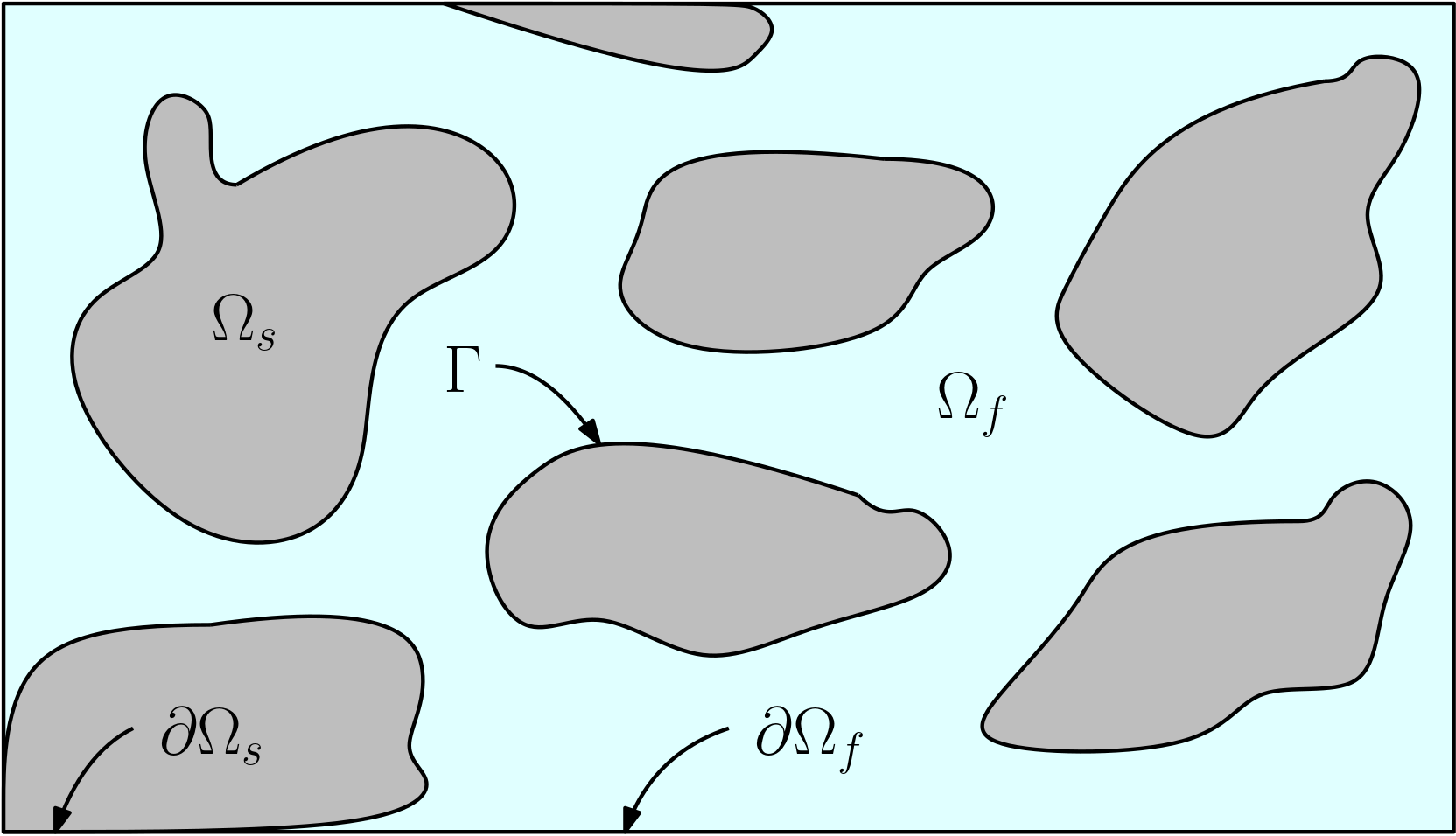
Figure 1: Graphical representation of the whole domain $\Omega=\Omega_{\text{s}}\cup\Omega_{\text{f}}$ considering two sub-domains: $\Omega_{\text{s}}$ a solid region (not necessarily connected), with external boundary $\partial\Omega_{\text{s}}$; and, $\Omega_{\text{f}}$ a fluid region with $\partial\Omega_{\text{f}}$ external boundary such that $\partial\Omega=\partial\Omega_{\text{s}}\cup\partial\Omega_{\text{f}}$. Solid-fluid interface denoted as $\Gamma$.

2.1 Stokes’ flow

Consider $\Omega_{\text{f}}$, with velocity profile $\mathbf{u}(\mathbf{x},t)$ governing the advective dynamics of the ions. Assume a negligible Reynolds numbers Re defined by the fluid density $\rho_{\text{f}}$, characteristic velocity $U$, characteristic length scale $L$ and dynamic viscosity $\mu$:

$$\textrm{Re}\mathrel{\mathop{\mathchar 58\relax}}=\frac{\rho_{\text{f}}LU}{\mu}\ll 1,$$

such that viscous forces within $\Omega_{\text{f}}$ outweigh the inertial. This common assumption in ionic transport [35, 15, 7] leads to linear Stokes flow. Furthermore, we assume the fluid to be incompressible, i.e.,

$$\mu\nabla^{2}\mathbf{u}=\bm{\nabla}{p}-\rho_{\text{el}}\mathbf{E}, \quad\mathbf{x}\in\Omega_{\text{f}},$$ (1)

$$\bm{\nabla}\cdot\mathbf{u}=0, \quad\mathbf{x}\in\Omega_{\text{f}},$$ (2)

where $p=p(\mathbf{x},t)$, $\displaystyle\rho_{\text{el}}=\rho_{\text{el}}(\mathbf{x},t)=F\sum_{i=1}^{N}z_{i}c_{i}$ and $\mathbf{E}$ are the static fluid pressure, electric charge density and electric field, respectively, and $F$ is Faraday’s constant. Compared to the standard Stokes equation, we have the presence of the body force term $\rho_{\text{el}}\mathbf{E}$, describing the Coulomb forces acted on the fluid by the ions[15, 31]. We neglect any magnetic contribution by assuming our ions move slowly such that $\mathbf{E}$ is irrotational, i.e. $\bm{\nabla}\times\mathbf{E}=\mathbf{0}$. This body force term may be set to zero if the fluid is unaffected by $\mathbf{E}$ or the fluid is approximated as electrically-neutral, $\rho_{\text{el}}=0$. This will be further discussed in §3.

The first coupling term, between the variables $\mathbf{u}$, $\mathbf{E}$ and $c_{i}$ appears here, showing one of the significant difficulties of describing electrokinetic flows. The coupling terms (particularly if non-linear) often add significant numerical difficulties. First of all, they make the velocity field time-dependent. Although by neglecting the time derivative we assume instantaneous relaxation to an equilibrium, and thereby a steady solution, by involving $c_{i}(\mathbf{x},t)$ the relaxation becomes tied to the time scale of Nernst-Planck, which is order magnitudes different. For segregated approaches, the disparity of relaxation time scales between Stokes, Poisson and Nernst-Planck – leading to mixed parabolic-elliptic systems – can pose severe instability problems or slow convergence of the coupled system.

2.2 Poisson’s equation

To model the electric field $\mathbf{E}$, neglecting magnetic forces, We may then write $\mathbf{E}=-\bm{\nabla}\phi$ and focus on the electric potential $\phi=\phi(\mathbf{x},t)$. Assume for each sub-domain their respective electric permittivity $\varepsilon$ is spatially constant. From Maxwell’s equations, we obtain Poisson’s electrostatic equation denoting variations in $\phi$ by changes in the charge density $\rho_{\text{el}}$,

$$\nabla^{2}\phi=-\frac{\rho_{\text{el}}}{\varepsilon}=-\frac{F}{\varepsilon}\sum_{i=1}^{N}z_{i}c_{i},\qquad\mathbf{x}\in\Omega_{\{\text{f,s}\}}.$$ (3)

where $\varepsilon=\varepsilon_{\text{s}}$ in the solid and $\varepsilon=\varepsilon_{\text{f}}$ in the fluid. Again we have direct coupling between our variables, here between $c_{i}$ and $\phi$, although this time the former appears linearly in the source term. Like for Stokes flow, this equation depends on time only through the source/coupling terms, in particular the time-dependent ionic concentration $c_{i}(\mathbf{x},t)$.

For a conductive material (e.g., solid electrode), assuming $\varepsilon\to\infty$ and Ohm’s law (linear relation between the potential gradient and the current density), the governing equation for the potential becomes:

$$\bm{\nabla}\cdot\sigma\bm{\nabla}\phi=0,$$ (4)

where $\sigma$ is the conductivity of the material.

2.3 Ionic transport

Assume the ionic fluid in $\Omega_{\text{f}}$ is sufficiently dilute to ignore ion-ion interactions and diffusion is isotropic. Under these assumptions we may use the Nernst-Planck flux [15, 30, 22, 10] as

$$\mathbf{j}_{i}=\mathbf{j}(c_{i},\phi)=\begin{cases}-D_{i\text{,s}}\left(\bm{\nabla}c_{i}\right)&\qquad\mathbf{x}\in\Omega_{\text{s}},\\ -D_{i,\text{f}}\left(\bm{\nabla}c_{i}+\frac{Fz_{i}}{RT}c_{i}\bm{\nabla}\phi\right)+\mathbf{u}c_{i}&\qquad\mathbf{x}\in\Omega_{\text{f}},\end{cases}$$ (5)

where denote $R$, $T$, $D_{i,\text{f}}$ and $D_{i,\text{s}}$ are, respectively, the ideal gas constant, absolute temperature and diffusion coefficient of species $i$ in the fluid and in the solid. Taking eq. 5 in conjunction with the continuity equation for mass conservation we arrive at the set of equations modelling transport of $c_{i}$,

$$\frac{\partial c_{i}}{\partial t}+\bm{\nabla}\cdot\mathbf{j}_{i}=0,\qquad\mathbf{x}\in\Omega_{\text{s,f}}.$$ (6)

As mentioned, we assume a dilute solution to ignore ion-ion interactions. This may not hold true in some cases. Alternatively the Stefan-Maxwell equations [32, 15, 16] may be used in lieu of Nernst-Planck. In short, Stefan-Maxwell balances the driving forces exerted on a species with the frictional forces between species. This introduces cross diffusivities $\mathcal{D}_{ij}$ describing the drag between species $i$ and $j$ due to these frictional forces [15]. The added complexity from such explicit coupling between species is difficult to describe, as the exact description of $\mathcal{D}_{ij}$ is hard to determine [32]. Even in situations where the ionic fluid is bordering on dilute, it is common for Nernst-Planck to still be used [33] due to its simplicity.

To close the system of equations listed here, we must include conditions along the boundaries of $\Omega_{\text{f}}$ and $\Omega_{\text{s}}$. We briefly discuss some common choices below and their physical representation. We also require conditions at the interface $\Gamma$ to describe the interaction between sub-domains. This is discussed further below for $c_{i}$ and $\phi$ when considering reactions and (non-)conductive interfaces.

2.4 Boundary conditions

Below we list some relevant conditions for different physical situations often seen in electrokinetic problems:

• Solid walls: Either a conductive or insulating wall. The no-penetration ($\mathbf{u}\cdot\mathbf{n}=0$, and zero normal stresses), where $\mathbf{n}$ is the outward unit normal to the boundary, or no-slip condition ($\mathbf{u}=\mathbf{0}$) may be used. Ions may not pass through the wall so their fluxes are zero ($\mathbf{j}_{i}\cdot\mathbf{n}=0$). If conductive we impose a fixed normal current density $I_{\text{w}}$ along the wall ($\displaystyle\mathbf{i}\cdot\mathbf{n}=F\sum_{i}z_{i}\mathbf{j}_{i}\cdot\mathbf{n}=I_{\text{w}}$ for a liquid electrolyte) or fixed potential $\phi_{\text{w}}$. If insulating (non-conductive) we may simply set $I_{\text{w}}=0$.

• Permeable membrane and reactive boundaries: For a membrane, we can fix the flux of each species ($\mathbf{j}_{i}\cdot\mathbf{n}=j_{\text{m}}$), non-zero for species capable of passing through, zero otherwise. We will discuss the case of reactive boundaries later in §4.2.

• Inlet/Outlet: Often used to model an in/out-flow of fluid and/or ions. For a momentum driven inlet, pressure or flow velocity may be fixed ($\mathbf{u}=\mathbf{u}_{\text{in}}$, $p=p_{\text{in/out}}$). For ions we may apply fixed fluxes ($\mathbf{j}_{i}\cdot\mathbf{n}=j_{\text{in/out}}$), resulting in a fixed electric current ($\displaystyle\mathbf{i}\cdot\mathbf{n}=I_{\text{in/out}}$). More complicated is to determine suitable boundary conditions for the potential. Typically, either a Dirichlet $\phi=\phi_{\text{in/out}}$ or a Neumann condition consistent with the ionic current can be imposed. The latter imposes the total electric current to be either equal to zero or a fixed value.

• Periodicity: when dealing with large (quasi-)periodic (or homogeneous) structures, it is often impossible to solve for the entire domain of interest. In these cases, smaller representative unit cells can be solved with (quasi-)periodic external boundary conditions [5] are imposed. In these cases, additional driving forces (as a bulk source term or a modification of the periodic BC) need to be added.

3 Dimensional analysis

When dealing with systems of coupled transport equations it is useful to perform a dimensional analysis to better understand the relationships between the different transport phenomena and identify the limiting regimes and possible approximations. We denote dimensionless variables with a hat symbol, e.g. $\hat{x}$, and reference values with a bar unless stated otherwise. We use the reference values $L$, $U$, $\bar{\phi}$ and $\bar{c}_{i}$ for the length scale, velocity, electric potential and concentrations respectively. For pressure, we take $\bar{p}=\frac{\mu U}{L}$ as this the appropriate form when under Stokes flow. For time, we take the diffusive timescale $\bar{t}=\frac{L^{2}}{D_{i}}$. With these choices and defining $\bar{C}=\displaystyle\frac{1}{2}\sum_{i=1}^{N}z_{i}^{2}\bar{c_{i}}$ as the reference total ionic strength, we obtain the dimensionless variables:

$$\hat{x}=\frac{x}{L},\quad\hat{t}=\frac{D_{i}t}{L^{2}},\quad\hat{\mathbf{u}}=\frac{\mathbf{u}}{U},\quad\hat{\phi}=\frac{\phi}{\bar{\phi}},\quad\hat{c_{i}}=\frac{c_{i}}{\bar{c_{i}}},\quad\hat{p}=\frac{pL}{\mu U}.$$ (7)

Substituting these dimensionless variables into eq. 1, eq. 3 and eq. 6 the dimensionless system of equations are

$$\frac{D_{i}\bar{c_{i}}}{L^{2}}\frac{\partial\hat{c_{i}}}{\partial\hat{t}} +\hat{\bm{\nabla}}\cdot\left(-D_{i}\left(\frac{\bar{c_{i}}}{L^{2}}\hat{\bm{\nabla}}\hat{c_{i}}+\frac{F\bar{\phi}\bar{c_{i}}}{L^{2}RT}\hat{c}_{i}z_{i}\hat{\bm{\nabla}}\hat{\phi}\right)+\frac{U\bar{c_{i}}}{L}\hat{c_{i}}\hat{\mathbf{u}}\right)=0,$$ (8)

$$\frac{\bar{\phi}}{L^{2}}\hat{\nabla}^{2}\hat{\phi} =-\frac{F}{\varepsilon}\sum_{i=1}^{N}z_{i}\hat{c_{i}}\bar{c_{i}},$$ (9)

$$\frac{\mu U}{L^{2}}\hat{\nabla}^{2}\hat{\mathbf{u}} =\frac{\mu U}{L^{2}}\hat{\bm{\nabla}}\hat{p}+\frac{F\bar{\phi}}{L}\hat{\bm{\nabla}}\hat{\phi}\sum_{i=1}^{N}z_{i}\hat{c}_{i}\bar{c_{i}}.$$ (10)

The underlying dimensionless numbers may be found by dividing all other terms by the reference values of one term. For eqs. 8, 9 and 10 we divide by $\frac{D_{i}\bar{c_{i}}}{L^{2}}$, $\frac{2\bar{C}F}{\varepsilon}$ and $\frac{2\bar{C}\mu U}{2\bar{C}L^{2}}$ respectively, where recall $\bar{C}$ is the reference ionic strength needed to resolve the issue of not being able to factor out the reference concentrations $\bar{c}_{i}$. As such, the dimensionless equations become:

$$\frac{\partial\hat{c_{i}}}{\partial\hat{t}}+\hat{\bm{\nabla}}\cdot\left(-\left(\hat{\bm{\nabla}}\hat{c_{i}}+\mathcal{N}\hat{c_{i}}z_{i}\hat{\bm{\nabla}}\hat{\phi}\right)+\textrm{Pe}_{i}\hat{\mathbf{u}}\hat{c_{i}}\right)=0,$$ (11)

$$\mathcal{L}^{2}\hat{\nabla}^{2}\hat{\phi}=-\frac{\sum_{i=1}^{N}\hat{c_{i}}\bar{c_{i}}z_{i}}{2\bar{C}},$$ (12)

$$\hat{\nabla}^{2}\hat{\mathbf{u}}=\hat{\bm{\nabla}}\hat{p}+\frac{\mathcal{P}}{2\bar{C}}\sum_{i=1}^{N}\hat{c_{i}}\bar{c_{i}}z_{i}\hat{\bm{\nabla}}\hat{\phi},$$ (13)

where we have defined four dimensionless numbers $\mathcal{N}$, Pe, $\mathcal{L}$ and $\mathcal{P}$. Note that whilst eq. 8 had four terms, we only arrive at two numbers due to our choice of reference time. The same can be said with eq. 13 and chosen reference pressure. This results in the following four dimensionless numbers for the three equations eq. 14 as:

$$\mathcal{N}=\frac{F\bar{\phi}}{RT}=\frac{e\bar{\phi}}{k_{\text{B}}T},\quad\textrm{Pe}=\frac{UL}{D_{i}},\quad\mathcal{L}^{2}=\frac{\varepsilon k_{\text{B}}T}{2N_{\text{A}}e^{2}L^{2}\bar{C}},\quad\mathcal{P}=\frac{2FL\bar{\phi}\bar{C}}{\mu U},$$ (14)

written in terms of the aforementioned reference values, where we denote $e$, $k_{\text{B}}$ and $N_{\text{A}}$ to be the elementary charge, Boltzmann’s constant and Avogadro’s number respectively. $\mathcal{N}$ represents the ratio of electrostatic over diffusive forces, with $\mathcal{N}\ll 1$ indicating diffusion is dominant. We also obtain the Péclet number Pe, i.e., the ratio of advective over diffusive phenomena, and $\mathcal{L}=\frac{\lambda_{\text{D}}}{L}$ the dimensionless Debye length, with the dimensional form $\lambda_{\text{D}}$ defined as

$$\lambda_{\text{D}}=\sqrt{\frac{\varepsilon k_{\text{B}}T}{2N_{A}e^{2}\bar{C}}}\,,$$ (15)

approximating the distance at which a charge’s electrostatic effect persists. Typically $\mathcal{L}\ll 1$, stating how the Debye length is much smaller than the reference length $L$. Finally, we have $\mathcal{P}$ denoting the ratio of viscous and electric forces upon our fluid. $\lambda_{\text{D}}$ is also the approximate width of a common electrokinetic phenomenon known as the electric double layer (EDL), see fig. 2, that forms on boundaries. The EDL consists first of ions adsorbed at the boundary, known as the Stern layer, and another of free ions moved by electrical attraction and diffusive motion by the Stern layer, deemed the diffuse layer.

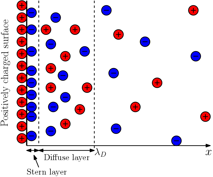
Figure 2: A graphical representation of the electric double layer along a positively charged surface, comprised of a thin layer of adsorbed negative ions (Stern layer) and loosely connected positive and negative ions (Diffuse layer).

For sufficiently thin EDLs there is a common model reduction known as the electro-neutrality assumption, often employed in the development of macroscopic models [33, 35, 17]. This reduction can in fact be determined through dimensional analysis and will be briefly discussed next.

3.1 Asymptotics and electro-neutrality

The electro-neutrality approximation states that for a sufficiently dilute electrolyte, all charges of ionic species within the solution roughly cancel each other out, leaving the solution electrically neutral. Electro-neutrality for a solution containing $N$ species is defined as

$$\sum_{i=1}^{N}z_{i}c_{i}=0,$$ (16)

and is often used as model reduction when modelling ionic flows. Where eq. 16 becomes invalid however is in the thin charged double layers, or EDL, mentioned above and often seen in real-world settings.

To get an understanding of where electro-neutrality comes from and how it relates to EDL formation, we perform an asymptotic analysis. Without any lack of generality, we limit here to a one-dimensional electrolyte and a binary electrolyte. In the numerical framework described above an arbitrary number of ionic species in three dimensions can be considered. Let $x\in\Xi$ where $\Xi=[0,1]$ is a binary electrolyte solution with ionic concentrations $c_{1}$ and $c_{2}$ of opposing valencies. For now, we omit any boundary conditions, only requiring these to result in a boundary layer formation near $x=0$. To arrive at eq. 16 we start by considering the asymptotics of the outer (bulk) layer away from $x=0$. For simplicity, we only consider the leading order terms.

Outer (bulk) layer:

To arrive at an asymptotic leading order solution in the bulk layer of $\Xi$ we take the following expansions of $\hat{u}$, $\hat{\phi}$, $\hat{p}$, $\hat{c_{1}}$ and $\hat{c_{2}}$. These denote the fluid velocity, electric potential, pressure and ion concentrations respectively, all dimensionless. Expansions are taken in powers of $\epsilon=\mathcal{L}^{2}$, the squared dimensionless Debye screening length since $\epsilon\ll 1$, or, $\lambda_{\text{D}}\ll L$:

$$\hat{\phi} =\phi^{(0)}+\epsilon\phi^{(1)}+\mathcal{O}(\epsilon^{2}),$$ (17)

$$\hat{c_{i}} =c_{i}^{(0)}+\epsilon c_{i}^{(1)}+\mathcal{O}(\epsilon^{2}),\quad i=1,2,$$ (18)

$$\hat{u} =u^{(0)}+\epsilon u^{(1)}+\mathcal{O}(\epsilon^{2}),$$ (19)

$$\hat{p} =p^{(0)}+\epsilon p^{(1)}+\mathcal{O}(\epsilon^{2}).$$ (20)

Substituting these expansions into the transport eqs. 11, 12 and 13 for one-dimension, alongside the incompressibility condition, we arrive at

$$\begin{split}&\mathcal{O}(\epsilon^{2})=\frac{\partial}{\partial t}\left(c_{i}^{(0)}+\epsilon c_{i}^{(1)}\right)+\frac{\partial}{\partial x}\bigg{(}\textrm{Pe}_{i}\left[u^{(0)}+\epsilon u^{(1)}\right]\left[c_{i}^{(0)}+\epsilon c_{i}^{(1)}\right]-\frac{\partial}{\partial x}\left(c_{i}^{(0)}+\epsilon c_{i}^{(1)}\right)\\ &\hskip 40.00006pt-\mathcal{N}z_{i}\left(c_{i}^{(0)}+\epsilon c_{i}^{(1)}\right)\frac{\partial}{\partial x}\left(\phi^{(0)}+\epsilon\phi^{(1)}\right)\bigg{)},\quad i=1,2,\end{split}$$ (21)

$$\mathcal{O}(\epsilon^{2})=\epsilon\frac{\partial^{2}}{\partial x^{2}}\left(\phi^{(0)}+\epsilon\phi^{(1)}\right)+\frac{1}{2\bar{C}}\sum_{i=1}^{2}z_{i}\bar{c_{i}}\left(c_{i}^{(0)}+\epsilon c_{i}^{(1)}\right),$$ (22)

$$\begin{split}&\mathcal{O}(\epsilon^{2})=-\frac{\partial^{2}}{\partial x^{2}}\left(u^{(0)}+\epsilon u^{(1)}\right)+\frac{\partial}{\partial x}\left(p^{(0)}+\epsilon p^{(1)}\right)\\ &\hskip 40.00006pt+\frac{\mathcal{P}}{2\bar{C}}\frac{\partial}{\partial x}\left(\phi^{(0)}+\epsilon\phi^{(1)}\right)\sum_{i=1}^{2}z_{i}\bar{c_{i}}\left(c_{i}^{(0)}+\epsilon c_{i}^{(1)}\right),\end{split}$$ (23)

$$\mathcal{O}(\epsilon^{2})=\frac{\partial}{\partial x}\left(u^{(0)}+\epsilon u^{(1)}\right).$$ (24)

By considering only the leading order terms i.e., terms of $\mathcal{O}(1)$, these equations reduce to,

$$\frac{\partial}{\partial t}c_{i}^{(0)}+\frac{\partial}{\partial x}\left(\textrm{Pe}_{i}u^{(0)}c_{i}^{(0)}-\frac{\partial}{\partial x}c_{i}^{(0)}-\mathcal{N}z_{i}c_{i}^{(0)}\frac{\partial}{\partial x}\phi^{(0)}\right)=0,\quad i=1,2,$$ (25)

$$0=z_{1}\bar{c_{1}}c_{1}^{(0)}+z_{2}\bar{c_{2}}c_{2}^{(0)},$$ (26)

$$\frac{\partial^{2}}{\partial x^{2}}u^{(0)}=\frac{\partial}{\partial x}p^{(0)},$$ (27)

$$\frac{\partial}{\partial x}u^{(0)}=0.$$ (28)

Note how eq. 26 is the electro-neutrality approximation mentioned before, for a binary solution, and a direct consequence of the asymptotics. This implies said electro-neutrality is only accurate up to leading order. The electric body force of Stokes vanishes as a consequence of eq. 26. To write an equation for the leading order potential $\phi^{(0)}$ we can multiply eq. 25 by their respective valencies $z_{i}$ and reference values $\bar{c_{i}}$, sum over $i$, and utilise eq. 26, resulting in the equation,

$$\frac{\partial}{\partial x}\left(u^{(0)}\sum_{i}\textrm{Pe}_{i}z_{i}\bar{c_{i}}c_{i}^{(0)}-\sum_{i}z_{i}\bar{c_{i}}\frac{\partial}{\partial x}c_{i}^{(0)}-\mathcal{N}\sum_{i}z_{i}^{2}\bar{c_{i}}c_{i}^{(0)}\frac{\partial}{\partial x}\phi^{(0)}\right)=0,$$ (29)

which represents a steady equation for $\phi^{(0)}$. This can be interpreted as a modified Ohm’s law with new conductivity accounting for all contributions to the total current: advective, diffusive and electrical, from left to right.

Now that we have constructed the asymptotic solution, up to $\mathcal{O}(1)$, for the outer (bulk) layer of $\Xi$, we move on to determine the inner (boundary) layer asymptotics. As mentioned at the start, we state said inner layer formation is near $x=0$ of $\Xi$. Much like the outer layer, we make no case of boundary conditions, only that a boundary layer near $x=0$ forms as a result of them.

Inner solution:

To construct a solution for the inner layer near $x=0$ of $\Xi$ we define the variable $y$ to span the inner layer and be a ’fast’ variable counterpart to $x$, changing more rapidly,

$$y=\frac{x}{\sqrt{\epsilon}},\quad y\in[0,\infty)\,.$$ (30)

By the definition of $x\in\Xi$, $y$ therefore has domain $[0,\infty)$, as $y=0$ for $x=0$ and $y\rightarrow\infty$ for $x\rightarrow 1$, since $\epsilon\ll 1$. Such change of variable gives derivatives via chain rule as:

$$\frac{\partial}{\partial x}=\frac{1}{\sqrt{\epsilon}}\frac{\partial}{\partial y},\quad\frac{\partial^{2}}{\partial x^{2}}=\frac{1}{\epsilon}\frac{\partial^{2}}{\partial y^{2}}.$$ (31)

Substitution of the above derivatives into the original transport equations eqs. 11, 12 and 13 results in,

$$\frac{\partial\hat{c_{i}}}{\partial\hat{t}}+\frac{1}{\sqrt{\epsilon}}\frac{\partial}{\partial y}\left(\textrm{Pe}_{i}\hat{u}\hat{c_{i}}-\frac{1}{\sqrt{\epsilon}}\frac{\partial\hat{c_{i}}}{\partial y}-\frac{1}{\sqrt{\epsilon}}\mathcal{N}z_{i}\hat{c_{i}}\frac{\partial\hat{\phi}}{\partial y}\right)=0,$$ (32)

$$\frac{\partial^{2}\hat{\phi}}{\partial y^{2}}=-\frac{1}{2\bar{C}}\sum_{i=1}^{2}z_{i}\bar{c_{i}}\hat{c_{i}},$$ (33)

$$\frac{1}{\epsilon}\frac{\partial^{2}\hat{u}}{\partial y^{2}}=\frac{1}{\sqrt{\epsilon}}\frac{\partial\hat{p}}{\partial y}+\frac{1}{\sqrt{\epsilon}}\frac{\mathcal{P}}{2\bar{C}}\frac{\partial\hat{\phi}}{\partial y}\sum_{i=1}^{2}z_{i}\bar{c_{i}}\hat{c_{i}},$$ (34)

$$\frac{\partial\hat{u}}{\partial y}=0,$$ (35)

where all variables $\hat{u}$, $\hat{p}$, $\hat{\phi}$ and $\hat{c_{i}}$ are in terms of y e.g., $\hat{c_{i}}=\hat{c_{i}}(y,t)$. Just like the outer layer, we substitute the asymptotic expansions eqs. 17, 18, 19 and 20 into the above equations to obtain,

$$\begin{split}\frac{\partial}{\partial t}\left(c_{i}^{(0)}+\epsilon c_{i}^{(1)}\right)&+\frac{1}{\sqrt{\epsilon}}\frac{\partial}{\partial y}\bigg{(}\textrm{Pe}_{i}\left[u^{(0)}+\epsilon u^{(1)}\right]\left[c_{i}^{(0)}+\epsilon c_{i}^{(1)}\right]-\frac{1}{\sqrt{\epsilon}}\frac{\partial}{\partial y}\left(c_{i}^{(0)}+\epsilon c_{i}^{(1)}\right)\\ &\quad-\mathcal{N}z_{i}\frac{1}{\sqrt{\epsilon}}\left(c_{i}^{(0)}+\epsilon c_{i}^{(1)}\right)\frac{\partial}{\partial y}\left(\phi^{(0)}+\epsilon\phi^{(1)}\right)\bigg{)}=\mathcal{O}(\epsilon^{2}),\quad i=1,2,\end{split}$$ (36)

$$\frac{\partial^{2}}{\partial y^{2}}\left(\phi^{(0)}+\epsilon\phi^{(1)}\right)=-\frac{1}{2\bar{C}}\sum_{i=1}^{2}z_{i}\bar{c_{i}}\left(c_{i}^{(0)}+\epsilon c_{i}^{(1)}\right)+\mathcal{O}(\epsilon^{2}),$$ (37)

$$\begin{split}\frac{1}{\epsilon}\frac{\partial^{2}}{\partial y^{2}}\left(u^{(0)}+\epsilon u^{(1)}\right)&=\frac{1}{\sqrt{\epsilon}}\frac{\partial}{\partial y}\left(p^{(0)}+\epsilon p^{(1)}\right)\\ &\quad+\frac{1}{\sqrt{\epsilon}}\frac{\mathcal{P}}{2\bar{C}}\frac{\partial}{\partial y}\left(\phi^{(0)}+\epsilon\phi^{(1)}\right)\sum_{i=1}^{2}z_{i}\bar{c_{i}}\left(c_{i}^{(0)}+\epsilon c_{i}^{(1)}\right)+\mathcal{O}(\epsilon^{2}),\end{split}$$ (38)

$$\frac{\partial}{\partial y}\left(u^{(0)}+\epsilon u^{(1)}\right)=\mathcal{O}(\epsilon^{2}).$$ (39)

Considering only the leading order terms of the four equations above we arrive at the following leading order set of equations for the inner layer:

$$\frac{\partial}{\partial y}\left(-\frac{\partial}{\partial y}c_{i}^{(0)}-\mathcal{N}z_{i}c_{i}^{(0)}\frac{\partial}{\partial y}\phi^{(0)}\right)=0,\quad i=1,2,$$ (40)

$$\frac{\partial^{2}}{\partial y^{2}}\phi^{(0)}=-\frac{1}{2\bar{C}}\sum_{i=1}^{2}z_{i}\bar{c_{i}}c_{i}^{(0)},$$ (41)

$$\frac{\partial^{2}}{\partial y^{2}}u^{(0)}=0,$$ (42)

$$\frac{\partial}{\partial y}u^{(0)}=0.$$ (43)

Like the outer layer equations, to close the system we need another equation, this time for $p^{(0)}$. Considering the $\mathcal{O}(\epsilon^{(1/2)})$ terms of eq. 38 we can retrieve such an equation as

$$\frac{\partial}{\partial y}p^{(0)}+\frac{\mathcal{P}}{2\bar{C}}\frac{\partial}{\partial y}\phi^{(0)}\sum_{i=1}^{2}z_{i}\bar{c_{i}}c_{i}^{(0)}=0.$$ (44)

As mentioned earlier, when considering situations involving multiple sub-domains we must also have appropriate interface conditions. In many real applications of electrokinetic flows, there are chemical reactions at interfaces between sub-domains, exchanging mass across the ionic species involved. In these cases, neglecting the EDL might lead to significant errors. In the next section, we will consider such reactions occurring on our interface $\Gamma$, formulating appropriate conditions to capture them whilst retaining mass conservation.

4 Multi-domain formulation and reactions

Here we formulate conditions to model heterogeneous reactions which are crucial for many electrochemical and electrokinetic problems. We write a general reaction rate that ensures total mass conservation and apply it to form reactive interface conditions, where we consider the scenarios of species that exist in the whole domain (unrestricted) or only in a specific sub-domain (restricted). We then discuss conditions on $\phi$ when the interface is conductive or non-conductive.

4.1 Reaction model

Consider a general elementary reaction transferring mass between reactants $i=J,...,K$ and products $i=K+1,...,M$ with exchanged molar masses $B_{i}$ and valencies $z_{i}$. We denote $\nu_{i}>0$ to be the stoichiometric coefficients determining the number of moles of species $i$ is lost or gained and $n$ the number of released ($n<0$) or absorbed ($n>0$) electrons, alongside the electron mass $e^{-}$. The mass balance of the reaction reads:

$$\sum_{i=J}^{K}\nu_{i}B_{i} +ne^{-}=\sum_{i=K+1}^{M}\nu_{i}B_{i}\,,$$ (45)

$$n =\sum_{i=K+1}^{M}z_{i}\nu_{i}-\sum_{i=J}^{K}\nu_{i}z_{i}.$$ (46)

To formulate eq. 45 as conditions on $\Gamma$ we first determine the rate $r_{i}$ at which each species in our reaction is exchanging mass. More complex reactions involving several intermediate reactions can be decomposed into elementary steps, i.e. a set of elementary reactions. Typically, the overall reaction rate is then given by the rate of the slowest elementary reaction [6]. One option to determine the rate is the law of mass action, also known as the rate law [2, 6]. Given an ideal solution and reaction involving chemical species $[j]$ with stoichiometric coefficients $\nu_{j}$, at dynamic equilibrium

$$\sum_{\text{reactants}}\nu_{j}[j]\rightleftharpoons\sum_{\text{products}}{\nu}_{j}[j]\,,$$ (47)

where the net reaction rate (density) $r^{\prime}$ with units [mol/m² s], is given by:

$$r^{\prime}=k_{\text{f}}\prod_{j}\bigg{(}c_{j}^{\nu_{j}}\bigg{)}_{\text{reac}}-k_{r}\prod_{j}\bigg{(}c_{j}^{\nu_{j}}\bigg{)}_{\text{prod}}\,.$$ (48)

Here $k_{\text{f}}$, $k_{\text{r}}$ are the rate constants for the forward and reverse reaction and can be empirically modelled by the Arrhenius equation [31, 6]. Note that $r^{\prime}$ is always positive, so we cannot simply take $r_{i}=r^{\prime}$ as we must allow $r_{i}<0$ for reactant species. Instead, we define the coefficient $\alpha_{i}$ as

$$\alpha_{i}=\begin{cases}-1&\text{reactants,}\\ +1&\text{products,}\end{cases}$$ (49)

and, multiplying by $r^{\prime}$ and $\nu_{i}$, we obtain:

$$r_{i}=\alpha_{i}\nu_{i}r^{\prime}=\alpha_{i}\nu_{i}\left(k_{\text{f}}\prod_{j=J}^{K}\bigg{(}c_{j}^{\nu_{j}}\bigg{)}_{\text{reac}}-k_{r}\prod_{j=K+1}^{M}\bigg{(}c_{j}^{\nu_{j}}\bigg{)}_{\text{prod}}\right),\qquad i=J,...,M.$$ (50)

For species not involved in the reaction we set $r_{i}=0$. Assuming a closed reactive system, i.e no trace ion species, we can represent the mass conservation as the balance across reaction rates $r_{i}$:

$$\sum_{i=1}^{N}m_{i}r_{i}=0.$$ (51)

We weigh by the molar masses $m_{i}$ to convert from moles (a non-conserved quantity between species) to grams. We use the rate law as the example here as it is valid for many reactions [6]. It is also the more general form for the commonly used Butler-Volmer equation for faradaic reactions, which uses the energy dependence of $k_{\text{f}}$ and $k_{\text{r}}$ to give explicit electric potential dependency. It is important to notice that the units of measure of the reaction rate are [mol/s] for bulk reactions and [m mol/s] for surface reactions. Therefore, for the case of linear reactions, the reaction constants $k_{i}$ can be either [1/s] or [m/s].

4.2 Interface conditions

The reaction models above can be applied in the bulk or on an interface. Here we apply them on $\Gamma$ for $\phi$ and $c_{i}$ given conductive or non-conductive interface and surface reactions respectively. We employ general reaction rates $r_{i}$ to balance the ionic fluxes $\mathbf{j}_{i}$ through $\Gamma$ with mass exchanged by the reaction. For $\phi$ we use conservation of charge to find conditions on the current passing through $\Gamma$ when acting conductively or non-conductively.

4.2.1 Interface conditions for ions concentration

Here we outline reactive conditions along $\Gamma$ to model eq. 45. We use a set of general, possibly non-linear, reaction rates $r_{i}$ for $i=J,\dots,M$ of ion species involved in eq. 45. We make no assumptions on the form of $r_{i}$, other than making sure eq. 51 holds true. For species not involved, we simply take flux continuity. The result, jump conditions in ionic flux between $\Omega_{\text{s}}$ and $\Omega_{\text{f}}$, equal to their respective reaction rates $r_{i}$:

$$\bigg{[}\mathbf{j}_{i}\cdot\mathbf{n}\bigg{]}^{\Gamma_{\text{s}}}_{\Gamma_{\text{f}}}=\begin{cases}r_{i}&\mathbf{x}\in\Gamma\text{ for }i=J,...,M,\\ \\ 0&\mathbf{x}\in\Gamma\text{ for }i\neq J,...,M.\end{cases}$$ (52)

Here we denote $\big{[}\mathbf{j}_{i}\cdot\mathbf{n}\big{]}_{\Gamma_{\text{f}}}$ to be the normal flux evaluated at $\Gamma$ from $\Omega_{\text{f}}$’s side. Alongside this we assume continuity of concentrations to provide our second condition:

$$c_{i}\big{\rvert}_{\Gamma_{\text{s}}}=c_{i}\big{\rvert}_{\Gamma_{\text{f}}},\quad\mathbf{x}\in\Gamma.$$ (53)

So, for all species involved in the reaction eq. 45 we have the difference in ionic flux from $\Omega_{\text{s}}$ and $\Omega_{\text{f}}$ to be the rate $r_{i}$ of the respective species. In some scenarios, one or more of the ion species may be restricted to reside in a single sub-domain of $\Omega$. This can however be easily modelled by simply modifying the conditions of those restricted species, setting both $\mathbf{j}_{i}$ and $c_{i}$ to be zero in the inaccessible domains.

4.2.2 Interface conditions for the potential

We consider conditions for the electric potential $\phi$ in different situations. Suppose our interface $\Gamma$ is allowing an electric current to flow through (e.g., an electrochemical reaction on the electrolyte side generating an electrical current in the solid electrode). The conservation of charge can be directly linked to Ohm’s law (for a solid electrode), i.e., the current through $\Gamma$ is proportional to the sum of changes in ionic fluxes, to provide an interface condition for the potential on the solid side:

$$F\sum_{i=1}^{N}z_{i}\bigg{[}\mathbf{j}_{i}\cdot\mathbf{n}\bigg{]}^{\Gamma_{\text{s}}}_{\Gamma_{\text{f}}}=\left|{\sigma\bm{\nabla}\phi\cdot\mathbf{n}}\right|_{\Gamma_{\text{s}}},\quad\mathbf{x}\in\Gamma.$$ (54)

In the electroneutral (outer expansion) approximation, the same condition can be also applied to the fluid side evaluating eq. 29 at $\Gamma$ and this closes the system. We see therefore that the conditions on the current are closely linked to the previous reactive conditions. If no reaction occurs at $\Gamma$, we simply have continuity of current due to ionic flux continuity. If a reaction is present, then eq. 52 tells us our jump in current is proportional to the sum of reaction rates $r_{i}$ alongside their respective charge numbers $z_{i}$. If $\Gamma$ is non-conductive instead, the current is zero, and we can impose a homogeneous Neumann condition for $\phi$ on conductive sides of $\Gamma$ (e.g., a solid electrode or an electroneutral electrolyte). This first interface condition need to be replaced by the continuity of the electric displacement field $\mathbf{D}=\varepsilon\bm{\nabla}\phi$ in case of non-electroneutral electrolytes (inner expansion) or dielectric media.

The second interface condition for the potential (not needed in the electroneutral approximation) comes from the definition of the potential jump across the interface. This can be related to the surface charge $\Sigma$ from Gauss’ law:

$$\bigg{[}\phi\bigg{]}^{\Gamma_{\text{s}}}_{\Gamma_{\text{f}}}=\frac{\Sigma}{\varepsilon_{\Gamma}},\quad\mathbf{x}\in\Gamma.$$ (55)

with $\varphi_{\Gamma}$ the permittivity of the interface. In this case the surface charge needs to be computed from the microscale local interface properties or assumed to be negligible, therefore resulting in the continuity of the potential across the interface.

5 Numerical implementation

As we have mentioned our goal is to construct simple, effective numerical solvers to the Stoke-Poisson-Nernst-Planck (SPNP) model at the pore scale. To do so, we employ the computational fluid dynamics (CFD) package OpenFOAM^® due to its open-source nature, large active community and robust handling of complex geometries. OpenFOAM^® is a finite volume library for general unstructured mesh. Coupled equations are solved iteratively in a segregated/splitted approach, solving sequentially each discretized equation. This removes the explicit coupling between equations, as well as the need of linearizing multi-linear terms (terms linear in each variable but where multiple variables appear) at the expense of having internal iterations. These would be unavoidable also if we adopted a monolithic approach due to the non-linearities of the model.

Two separate solvers have been implemented. The first, pnpFoam, models electrokinetic flow of a single ionic fluid, modelled by SPNP. The second, pnpMultiFoam, is more generalized, modelling a general set of ionic fluids and solids following SPNP and diffusion respectively. Furthermore, we developed the numerical counterpart, named mappedChemicalKinetics, to the reactive conditions in §4.2.1 for the case of a binary reaction. In this section, we will describe in detail the structure of the solvers and the corresponding boundary conditions.

5.1 Single- and multi-domain solvers

OpenFOAM^® discretizes each equation using a sparse matrix $\mathbf{M}$ with entries relating to the cell centres of the mesh. For example, for the fluid momentum, the discrete form reads:

$$\mathbf{M}[\mathbf{u}]=-\bm{\nabla}p-\rho_{\text{el}}\bm{\nabla}\phi,$$ (56)

where $[\mathbf{u}]$ is the vector of unknown velocities at cell centres and $\mathbf{M}$ is the coefficient matrix scaling the effect of neighbouring cell velocities. Note the right-hand terms are left as source terms and are computed explicitly and the gradient operators can be discretized with different schemes (details about the schemes will be presented in the results section). To solve for the pressure-velocity coupling we employ the PIMPLE algorithm with an extra term due to the electric body force. This works by decomposing $\mathbf{M}$ into its diagonal, $A$, and off-diagonal, $\mathbf{H}$, parts $\mathbf{M}[\mathbf{u}]=A\mathbf{u}-\mathbf{H}$. This leads to the velocity correction equation:

$$\mathbf{u}=\frac{\mathbf{H}}{A}-\frac{1}{A}\bm{\nabla}p-\frac{1}{A}\rho_{\text{el}}\bm{\nabla}\phi.$$ (57)

Interpolating $\mathbf{u}$ to the cell faces and taking the dot product with cell face area vectors $\mathbf{S}_{\text{f}}$ leads to the flux $U$ correction equation,

$$U=\mathbf{u}_{\text{f}}\cdot\mathbf{S}_{\text{f}}=\left(\frac{\bm{H}}{A}\right)_{\text{f}}\cdot\bm{S}_{\text{f}}-\left(\frac{1}{A}\right)_{\text{f}}\bm{S}_{\text{f}}\cdot\bm{\nabla}^{\perp}_{\text{f}}p^{n+1}-\left(\frac{\rho_{\text{el}}\bm{\nabla}\phi}{A}\right)_{\text{f}}\cdot\bm{S}_{\text{f}},$$ (58)

where subscript f denotes values at cell faces. Discretising the incompressibility condition $\bm{\nabla}\cdot\mathbf{u}=0$ gives $\bm{\nabla}\cdot U=0$ which when applied to the flux correction equation forms the pressure correction equation:

$$\bm{\nabla}\cdot\left(\left[\frac{\mathbf{H}}{A}\right]_{\text{f}}\bm{\nabla}p\right)=\bm{\nabla}\cdot\left(\left[\frac{\mathbf{H}}{A}\right]_{\text{f}}-\left[\frac{\rho_{\text{el}}\bm{\nabla}\phi}{A}\right]_{\text{f}}\right).$$ (59)

This is solved iteratively until convergence. In an external loop, momentum and pressure equations are coupled with the concentration and potential equations. When the mesh is highly skewed, or for complex discretisation schemes with implicit-explicit terms, additional iterations can be added for each single equation. The pseudo-code algorithm for our single ionic fluid solver pnpFoam is presented in Algorithm 1.

Construct fields: $\mathbf{u}$, $p$, $\phi$, $c_{i}$;

while $t<$ end time do

       while !converged do

             Initialize $\mathbf{u}^{n+1}$, $p^{n+1}$ to previous values: $\mathbf{u}^{n+1}=\mathbf{u}^{n}$, $p^{n+1}=p^{n}$;

             Solve momentum equation for $\mathbf{u}^{n+1}$: $-\mu\nabla^{2}\mathbf{u}^{n+1}+\rho_{\text{el}}\bm{\nabla}\phi=-\bm{\nabla}p^{n+1}$;

             while Pressure correction do

                   Solve pressure correction equation: $\bm{\nabla}\cdot\left[\left(\frac{1}{A}\right)_{\text{f}}\bm{\nabla}p^{n+1}\right]=\bm{\nabla}\cdot\left(\left(\frac{\bm{H}}{A}\right)_{\text{f}}-\left(\frac{\rho_{\text{el}}\bm{\nabla}\phi}{A}\right)_{\text{f}}\right)$;

                   Correct flux: $U^{n+1}=\mathbf{u}_{\text{f}}\cdot\bm{S}_{\text{f}}=\left(\frac{\bm{H}}{A}\right)_{\text{f}}\cdot\bm{S}_{\text{f}}-\left(\frac{1}{A}\right)_{\text{f}}\bm{S}_{\text{f}}\cdot\bm{\nabla}^{\perp}_{\text{f}}p^{n+1}-\left(\frac{\rho_{\text{el}}\bm{\nabla}\phi}{A}\right)_{\text{f}}\cdot\bm{S}_{\text{f}}$;

                   Correct velocity: $\mathbf{u}^{n+1}=\frac{\bm{H}}{A}-\frac{1}{A}\bm{\nabla}p^{n+1}-\frac{\rho_{\text{el}}\bm{\nabla}\phi}{A}$

             end while

            while Non-orthogonal correction do

                   Solve Poisson’s: $-\varepsilon\nabla^{2}\phi=\rho_{\text{el}}$;

                  

             end while

            for All $c_{i}$’s do

                   while Non-orthogonal correction do

                         Solve Nernst-Planck: $\frac{\partial c_{i}}{\partial t}+\bm{\nabla}\cdot\left(\mathbf{u}c_{i}-D_{i}\left(\bm{\nabla}c_{i}+\frac{F}{RT}z_{i}c_{i}\bm{\nabla}\phi\right)\right)=0$;

                        

                   end while

                  

             end for

            

       end while

      Increment time: $t\rightarrow t+\Delta t$

end while

Algorithm 1 pnpFoam algorithm

The same method is employed within the algorithm of pnpMultiFoam, our solver for ionic transport over a general set of ionic fluids and solids, where each region is solved separately, and an additional outer loop is added to ensure the coupling between regions. The algorithm is presented in Algorithm 2. Both solvers here are presented for the case of a non-electroneutral solution. In case electroneutrality is assumed, the algorithm is slightly modified to solve a modified potential equation eq. 29 (with ionic conductivity instead of permittivity) and with the last species calculated to ensure electro-neutrality.

Construct fields: $\mathbf{u}$, $p$, $\phi_{\text{f}}$, $\phi_{\text{s}}$, $c_{i,\text{f}}$, $c_{i,\text{s}}$;

while $t<$ end time do

       for All fluid regions do

             Initialize $\mathbf{u}^{n+1}$, $p^{n+1}$ to previous values: $\mathbf{u}^{n+1}=\mathbf{u}^{n}$, $p^{n+1}=p^{n}$;

             Solve momentum equation for $\mathbf{u}^{n+1}$ prediction : $-\mu\nabla^{2}\mathbf{u}^{n+1}+\rho_{\text{el}}\bm{\nabla}\phi=-\bm{\nabla}p^{n+1}$;

             while Pressure correction do

                   Solve pressure correction equation: $\bm{\nabla}\cdot\left[\left(\frac{1}{A}\right)_{\text{f}}\bm{\nabla}p^{n+1}\right]=\bm{\nabla}\cdot\left(\frac{\bm{H}}{A}\right)_{\text{f}}$;

                   Correct flux: $\mathbf{U}^{n+1}=\mathbf{u}_{\text{f}}\cdot\bm{S}_{\text{f}}=\left(\frac{\bm{H}}{A}\right)_{\text{f}}\cdot\bm{S}_{\text{f}}-\left(\frac{1}{A}\right)_{\text{f}}\bm{S}_{\text{f}}\cdot\bm{\nabla}^{\perp}_{\text{f}}p^{n+1}$;

                   Correct velocity: $\mathbf{u}^{n+1}=\frac{\bm{H}}{A}-\frac{1}{A}\bm{\nabla}p^{n+1}$

             end while

            while Non-orthogonal correction do

                   Solve Poisson’s: $-\varepsilon\nabla^{2}\phi_{\text{f}}=\rho_{\text{el}}$;

                  

             end while

            for All $c_{i,\textnormal{f}}$’s do

                   while Non-orthogonal correction do

                         Solve Nernst-Planck: $\frac{\partial c_{i,\textnormal{f}}}{\partial t}+\bm{\nabla}\cdot\left(\mathbf{u}c_{i,\textnormal{f}}-D_{i}\left(\bm{\nabla}c_{i,\textnormal{f}}+\frac{F}{RT}z_{i}c_{i,\textnormal{f}}\bm{\nabla}\phi_{\text{f}}\right)\right)=0$;

                        

                   end while

                  

             end for

            

       end for

      for All solid regions do

             while Non-orthogonal correction do

                   Solve Poisson’s: $-\varepsilon\nabla^{2}\phi_{\text{s}}=\rho_{\textnormal{el}}$;

                  

             end while

            for All $c_{i,s}$’s do

                   while Non-orthogonal correction do

                         Solve Diffusion equation: $\frac{\partial c_{i,\textnormal{s}}}{\partial t}-D_{i}\nabla^{2}c_{i,\textnormal{s}}=0$;

                        

                   end while

                  

             end for

            

       end for

      Increment time: $t\rightarrow t+\Delta t$;

      

end while

Algorithm 2 pnpMultiFoam algorithm

5.2 Boundary and interface conditions

To make use of the object orientation of OpenFOAM^® , all conditions are first reformulated as effective Robin conditions. We consider here, as an example, the inhomogeneous Robin BC for a variable $c$ with coefficients $D^{\star}$, $K^{\star}$ and $F^{\star}$ along a boundary $\Gamma$ with normal $\mathbf{n}$:

$$D^{\star}\bm{\nabla}_{\mathbf{n}}c\rvert_{\Gamma}=-K^{\star}c\rvert_{\Gamma}-F^{\star}\,.$$ (60)

In OpenFOAM^®   the boundary values $c\rvert_{\Gamma}$ and $\bm{\nabla}_{\mathbf{n}}c\rvert_{\Gamma}$ are approximated using the value of the cell centres with faces along $\Gamma$:

$$c\rvert_{\Gamma} \approx\alpha_{1}c_{c}+\alpha_{2},$$ (61)

$$\bm{\nabla}_{\mathbf{n}}c\rvert_{\Gamma} \approx\alpha_{3}c_{c}+\alpha_{4}\approx B(c_{\text{f}}-c_{c})\,.$$ (62)

Here $c_{\text{c}}$ and $c_{\text{f}}$ are the values of $c$ at the cell centre and face respectively. The $\alpha$’s are the interpolation weights, and $B$ is the inverse distance between the cell centre and the boundary. We can then rearrange eq. 60 using eqs. 61 and 62 to find the $\alpha$ values that allow us to approximate eq. 60 using the cell centres $c_{\text{c}}$:

$$\alpha_{1}=\frac{D^{\star}B}{D^{\star}B-K^{\star}}\>,\alpha_{2}=\frac{F^{\star}}{D^{\star}B-K^{\star}}\>,\alpha_{3}=\frac{K^{\star}B}{D^{\star}B-K^{\star}}\>,\alpha_{4}=\frac{F^{\star}B}{D^{\star}B-K^{\star}}\,.$$ (63)

This forms the basis of the Robin BC implemented. Reformulating all other conditions into a form like eq. 60 lets us reuse the same equations in eq. 63 to approximate all other conditions.

The interface conditions are implemented as a derived class named mappedChemicalKinetics. If we consider here the limiting case of two reacting species $c_{\text{s}}$ and $c_{\text{f}}$, each restricted to their respective sub-domains $\Omega_{\text{s}}$ and $\Omega_{\text{f}}$ respectively. Along the interface $\Gamma$ connecting the two sub-domains is the reaction:

$$\ce{\beta_{\text{s}}X_{\text{s}}<->\beta_{\text{f}}X_{\text{f}}}\,.$$ (64)

The general reactive conditions eq. 52 in this case reduces to the following condition along $\Gamma$:

$$\mathbf{j}_{\text{f}}\rvert_{\Gamma_{\text{f}}}\cdot\mathbf{n}=\mathbf{j}_{\text{s}}\rvert_{\Gamma_{\text{s}}}\cdot\mathbf{n}=r(c_{\text{f}}\rvert_{\Gamma_{\text{f}}},c_{\text{s}}\rvert_{\Gamma_{\text{s}}}),$$ (65)

where we denote here $\Gamma_{\text{s}}$ to be evaluation at the $\Omega_{\text{s}}$ side of $\Gamma$ and $\mathbf{n}$ the unit normal of $\Gamma$ facing into $\Omega_{\text{f}}$. Note the reaction rate $r$ is kept general and not necessarily linear. Equation 65 is solved iteratively using the Newton-Raphson method, linearised about the previous solution $\mathbf{c}^{N}=(c_{\text{s}}^{N}\hskip 5.0ptc_{\text{f}}^{N})^{\top}$. Here the previous solution could be the solution at the previous time step (if an explicit time stepping is chosen) or at the previous internal iteration (for fully implicit time stepping). This allows us to rewrite eq. 65 into two decoupled effective Robin conditions for $c_{\text{s}}^{N+1}$ and $c_{\text{f}}^{N+1}$ that we solve separately. The coupling between the two sides of the interface conditions (and therefore the two domains) is achieved through the internal iterations but, for stiff reactions, additional sub-looping to update both boundary values whenever one of the two domains is solved for. In algorithm 3 we detail the mappedChemicalKinetics pseudo-code to solve the effective Robin conditions. As both resulting effective Robin conditions are solved in the same manner we only write here solving of the condition for $c_{\text{f}}$.

Set tolerance: tol;

Set max Newton iterations: $N_{\text{max}}$;

Reset iterator: $N=0$;

while $||c_{\textnormal{f}}^{N}-c_{\textnormal{f}}^{N+1}||$ > tol $\cap$ $N\leq N_{\textnormal{max}}$ do

       Store previous iteration: $c_{\textnormal{f}}^{N}=c_{\textnormal{f}}^{N+1}$;

       Extract the face and internal values of the neighbouring field (solid side);

       Update $D^{*}_{\textnormal{f}}$, $K^{*}_{\textnormal{f}}$ and $F^{*}_{\textnormal{f}}$: see eqs. 108, 109 and 110 ;

       Evaluate iterative effective Robin BC: $-D^{*}_{\textnormal{f}}\bm{\nabla}_{\mathbf{n}}c_{\textnormal{f}}^{N+1}=-K^{*}_{\textnormal{f}}c_{\textnormal{f}}^{N+1}-F^{*}_{\textnormal{f}}$;

       Apply the boundary condition to obtain the new value: $c_{\textnormal{f}}^{N+1}$;

       if Stiff then

            Call mappedChemicalKinetics BC on the solid side;

       end if

      Increment iterator: $N\rightarrow N+1$

end while

Algorithm 3 mappedChemicalKinetics

More details about the linearization can be found in appendix A. Alongside the reactive conditions, we have also implemented a number of simpler conditions, such as the continuity of total fluxes, continuity of value or continuity of derivatives, often used within applications. Just as with the non-linear reactive condition, we rewrite all conditions into effective Robin conditions.

6 Numerical examples

Here we present four numerical examples of electrokinetic flows. To verify the accuracy of results we compare with the spectral Matlab^®  toolbox Chebfun [9] with machine-precision accuracy. The first case verifies the accuracy of the flow description given a single ion species using a pressure-driven infinite ion channel similar to [4]. Next, we verify accuracy when considering multiple ion species. Afterwards, we verify the implemented reactive interface conditions counterpart to §4.2.1. The final case displays the capabilities of our solver(s), simulating ionic transport within a randomized solid-fluid porous medium.

To show spatial convergence of OpenFOAM^® results we use the following normalized $L^{2}$ error point norm. We use here the dummy variables $v$ and $v_{\text{cref}}$ to denote OpenFOAM^® and Chebfun results respectively as an example:

$$L^{2}\text{-norm error }=\frac{\lVert v-v_{\text{cref}}\rVert_{2}}{\lVert v_{\text{cref}}\rVert_{2}}.$$ (66)

6.1 SPNP in an infinite channel

To verify pnpFoam and pnpMultiFoam for a single ion species take $\Omega$, of length $L$, with two boundaries $\Gamma_{\text{t}}$ and $\Gamma_{\text{b}}$ denoting the top and bottom channel walls respectively. Take boundaries $\Gamma_{\text{in}}$ and $\Gamma_{\text{out}}$ denoting the inlet and outlet of fluid in $\Omega$. To mathematically describe this channel as infinite we take periodic conditions on $\Gamma_{\text{in}}$ and $\Gamma_{\text{out}}$.

Figure 3: Graphical representation of the infinite ion channel with channel width $H$.

Take a monovalent ionic fluid, i.e a single ion species $c$ with valency $z=1$. Enforce a fixed external force $\mathbf{J}=\bigg{(}\begin{smallmatrix}-\mu/H^{2}\\ 0\end{smallmatrix}\bigg{)}$ to induce transport across the channel length. To allow electro-migration of $c$ between the two channel walls, fix $\phi=0.1$ along $\Gamma_{\text{t}}$ and $\phi=0$ on $\Gamma_{\text{b}}$. For $c$ apply no-flux along $\Gamma_{\text{t}}$ and $\Gamma_{\text{b}}$, denoting $\mathbf{n}$ to be the outward unit normal of either $\Gamma_{\text{t}}$ or $\Gamma_{\text{b}}$. We consider the channel at steady state and, by assuming $L$ is sufficiently large, take all derivatives in $x$ to be zero, i.e. $\frac{\partial a}{\partial x}=0$ for $a\in\{\mathbf{u},\phi,c,p\}$. Just like Poiseuille flow we assume a uni-directional velocity, such that $\mathbf{u}=\left(\begin{smallmatrix}u_{1}\\ 0\end{smallmatrix}\right)$. These assumptions in turn produce a one-dimensional reduce system of equations in $y$.

The SPNP system with a single ionic species in an infinite channel is considered with an added pressure-driven driving force $\mathbf{J}$:

$$\mu\nabla^{2}\mathbf{u}-\mathbf{J}-\bm{\nabla}p-Fc\bm{\nabla}\phi=0\,,\qquad \mathbf{x}\in\Omega,$$ (67)

$$\bm{\nabla}\cdot\mathbf{u}=0\,,\qquad \mathbf{x}\in\Omega,$$ (68)

$$\epsilon\nabla^{2}\phi+Fc=0\,,\qquad \mathbf{x}\in\Omega,$$ (69)

$$\bm{\nabla}\cdot\left[-D\left(\bm{\nabla}c+\frac{F}{RT}c\bm{\nabla}\phi\right)+\mathbf{u}c\right]=0\,,\qquad \mathbf{x}\in\Omega,$$ (70)

$$\mathbf{u}=\mathbf{0}\,,\quad\phi=0.05\,,\qquad \mathbf{x}\in\Gamma_{\text{t}}$$ (71)

$$\mathbf{u}=\mathbf{0}\,,\quad\phi=0\,,\qquad \mathbf{x}\in\Gamma_{\text{b}},$$ (72)

$$-D\bigg{(}\bm{\nabla}_{\mathbf{n}}c+\frac{F}{RT}c\bm{\nabla}_{\mathbf{n}}\phi\bigg{)}+c\mathbf{u}\cdot\mathbf{n}=0\,,\qquad \mathbf{x}\in\Gamma_{\text{b}}\cup\Gamma_{\text{t}},$$ (73)

$${a}\bigg{\rvert}_{\Gamma_{\text{in}}}={a}\bigg{\rvert}_{\Gamma_{\text{out}}}\,,\frac{\partial a}{\partial x}\bigg{\rvert}_{\Gamma_{\text{in}}}=\frac{\partial a}{\partial x}\bigg{\rvert}_{\Gamma_{\text{out}}}\,,\qquad a\in\{c,\mathbf{u},\phi,p\}.$$ (74)

The complete system is solved in OpenFOAM^® in a periodic channel, and compared with the equivalent one-dimensional model. By applying the assumptions of uni-directional flow and zero derivatives in $x$ we obtain a one-dimensional reduced set of equations in $y$:

$$\mu\frac{d^{2}u_{1}}{dy^{2}}=-\frac{\mu}{H^{2}}, \qquad\mathbf{x}\in\Omega,$$ (75)

$$0=\frac{dp}{dy}+Fc\frac{d\phi}{dy}, \qquad\mathbf{x}\in\Omega,$$ (76)

$$\varepsilon\frac{d^{2}\phi}{dy^{2}}=-Fc, \qquad\mathbf{x}\in\Omega,$$ (77)

$$0=\frac{d^{2}c}{dy^{2}}+\frac{F}{RT}\left(\frac{dc}{dy}\frac{d\phi}{dy}+c\frac{d^{2}\phi}{dy^{2}}\right), \qquad\mathbf{x}\in\Omega,$$ (78)

$$u_{1}=0,\,\phi=0.05, \qquad\mathbf{x}\in\Gamma_{\text{t}},$$ (79)

$$u_{1}=0,\,\phi=0, \qquad\mathbf{x}\in\Gamma_{\text{b}},$$ (80)

$$\frac{dc}{dy}+\frac{F}{RT}c\frac{d\phi}{dy}=0, \qquad\mathbf{x}\in\Gamma_{\text{b}}\cup\Gamma_{\text{t}},$$ (81)

where we excluded the incompressibility condition as this is trivially satisfied.

To compare results between Chebfun and our single ionic fluid solver pnpFoam we the following dimensionless numbers, geometrical parameters and transport properties, according to Table 1.

Symbol	$\mu$	$H$	$\varepsilon$	$\mathcal{N}$	Pe	$\mathcal{L}^{2}$	$\mathcal{P}$
Value	$10$	$1\times 10^{-6}$	$40\varepsilon_{0}$	$1.95$	$1.25\times 10^{5}$	$0.09$	$3.85\times 10^{-6}$

Table 1: Dimensionless numbers, domain and transport properties for the SPNP equation in the infinite channel. We denote $\varepsilon_{0}=8.85\times 10^{-12}$ to be the permittivity of vacuum.

When running pnpFoam we solve it in a steady state and take a large number of PIMPLE corrector iterations to ensure convergence of the coupled system. The mesh used in OpenFOAM^® is up to $N=420$ cells ($100$ in $x$, $320$ in $y$). Comparison of results and the $L^{2}$ error norm convergence are shown in fig. 4(b). We observe an accumulation of $c$ along $\Gamma_{\text{b}}$, causing a large pressure gradient to form. The velocity profile follows a parabolic arc, as expected, whilst we see a non-linear profile for $\phi$. Overall we find good agreement, with linear order spatial convergence $\mathcal{O}(N^{-1})$.

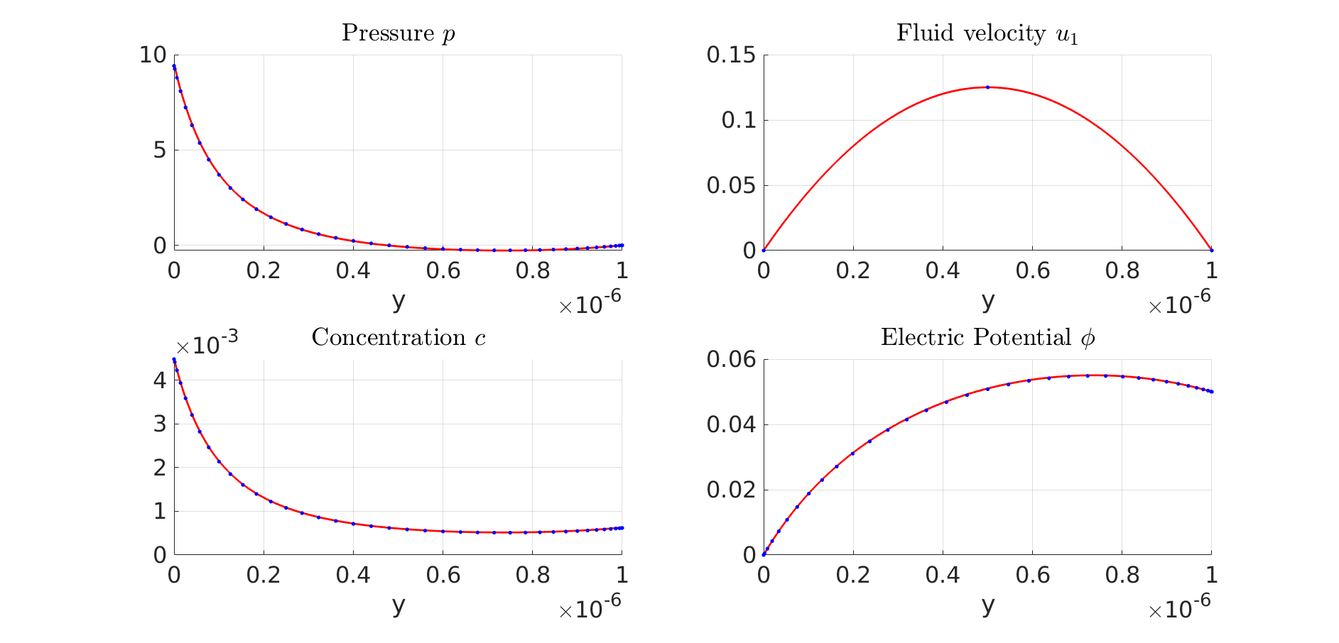
(a) Comparison of Chebfun (blue dots) and pnpFoam (red line) of the pressure, fluid velocity, ion concentration, and electric potential respectively, along the channel width i.e., in $y$.

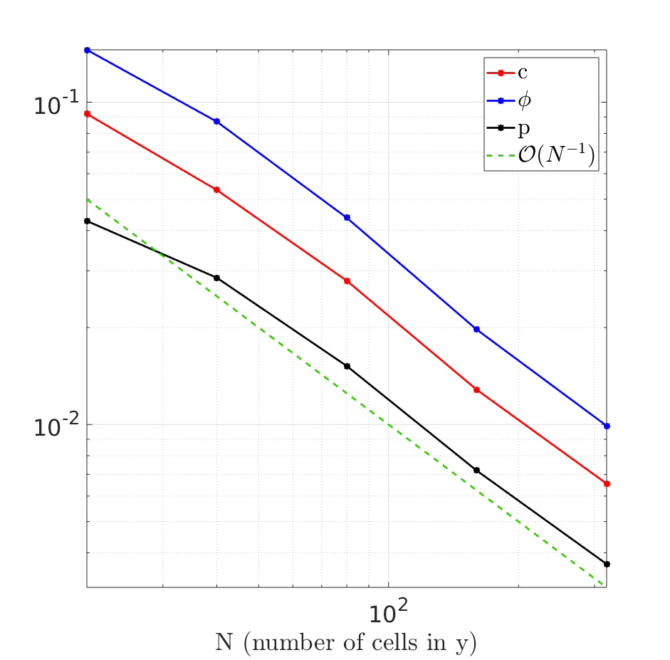
(b) $L^{2}$ error norm convergence plot of pnpFoam results, showing spatial convergence of $\mathcal{O}(N^{-1})$

6.2 Multi-component ionic fluid

To verify pnpFoam and pnpMultiFoam for a multi-component fluid we take two species $c_{1}$ and $c_{2}$ with opposite valencies $z_{1}=-z_{2}=1$ over the domain $\Omega\in[0,L]$ where $L=1\times 10^{-6}$. We set a zero-flux BC, i.e., $j(c_{i})=0$ at $x=0,L$ for both species and fix $\phi=0.1$ at $x=L$ and $\phi=0$ at $x=0$. We fix here a constant velocity $\mathbf{u}=0.001$ for simplicity, and we bypass the solution of the Stokes system (frozenFlow flag). Concentrations and potential are initially set to $c_{i}=1\times 10^{-3}$ and $\phi=0.05(1-\cos{\frac{\pi x}{L}})$.

We consider here the dimensionless number values in Table 2, indicating electrostatic forces dominate. From $\mathcal{L}$ we find the Debye length as approximately $\lambda_{\text{D}}=$308\text{\,}\mathrm{nm}$$. Since we are fixing $\mathbf{u}$ and neglecting Stokes we have $\mathcal{P}=0$.

Symbol	$\mathcal{N}$	Pe	$\mathcal{L}$	$\mathcal{P}$
Value	$3.868$	$1\times 10^{-3}$	$9\times 10^{-3}$	$0$

Table 2: Dimensionless numbers and parameters for the multi-component ionic fluid testcase.

When running pnpFoam we use a time step $\Delta t=10^{-7}$s, end time $t=1\times 10^{-5}$s, third-order implicit time scheme (backward keyword) and a mesh of up to $N=1000$ cells. Results and $L^{2}$ norm convergence plots are depicted in fig. 5(c) where we find good agreement of results and linear spatial convergence of all fields.

We see the ions are transported to the outer walls due to the high electric potential gradient. Most of the ions then accumulate within $\lambda_{\text{D}}$ from the walls forming two overlapping EDLs. Non-linear behaviour between $c_{i}$ and $\phi$ is observed through the slight shift in $\phi$’s profile due to the clustering of ions at the walls.

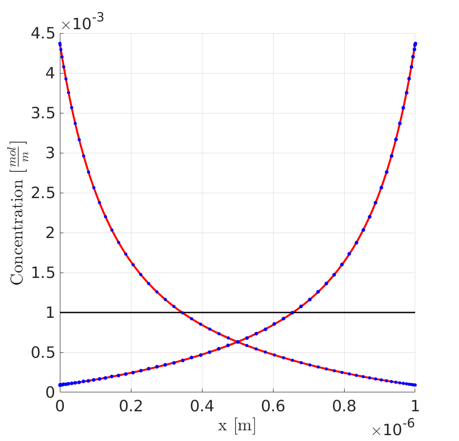
(a) Results of $c_{1}$ (left curve) and $c_{2}$ (right) at $t=1\times 10^{-5}$s. Blue and red denote Chebfun and pnpFoam results respectively. Black is the initial condition.

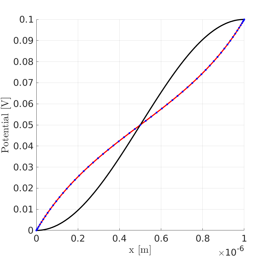
(b) Results of $\phi$ for Chebfun (blue) and pnpFoam (red) at $t=1\times 10^{-5}$s, with initial condition in black.

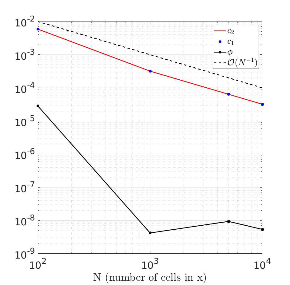
(c) $L^{2}$ point error norm convergence plot, showing $\mathcal{O}(N^{-1})$ spatial convergence of pnpFoam.

6.3 Reactive interface

Here we verify the accuracy of mappedChemicalKinetics, the numerical counterpart to the conditions found in §4.2.1. Consider the domain $\Omega=\Omega_{\text{s}}\cup\Omega_{\text{f}}=[-1,1]$ split into fluid $\Omega_{\text{f}}\in[-1,0]$ and solid $\Omega_{\text{s}}\in[0,1]$, each containing the species $c_{\text{f}}$ and $c_{\text{s}}$ respectively. Both species are restricted to their respective sub-domain, i.e. $c_{\text{s}}=0$ in $\Omega_{\text{f}}$ and vice versa. Consider the following elementary reaction at the $x=0$ interface:

$$[\text{s}]\leftrightharpoons[\text{f}].$$ (82)

As $c_{\text{s}}$ and $c_{\text{f}}$ are restricted to $\Omega_{\text{s}}$ and $\Omega_{\text{f}}$ respectively the reactive conditions of eqs. 52 and 53 become

$$j(c_{\text{f}}) =j(c_{\text{s}}),\quad x=0,$$ (83)

$$j(c_{\text{f}}) =k_{\text{f}}c_{\text{s}}-k_{\text{r}}c_{\text{f}},\quad x=0,$$ (84)

where we have used the linear rate law to model the reaction rate. Note $c_{\text{f}}$ and $c_{\text{s}}$ in eqs. 83 and 84 are evaluated on $\Omega_{\text{f}}$ and $\Omega_{\text{s}}$’s side of $x=0$ respectively. We set both species as uncharged, i.e. $z_{i}=0$, to remove electrostatic effects and $u=1$ in $\Omega_{\text{f}}$ to ignore Stokes. We initially set $c_{\text{s}}=0$ in $\Omega_{\text{s}}$ and $c_{\text{f}}=e^{-200(x+0.5)^{2}}$ in $\Omega_{\text{f}}$ so that a clear increase in $c_{\text{s}}$ can be seen.

Figure 6: Graphical representation of domain $\Omega$ containing a solid and fluid with zero flux outer boundaries and reactive flux conditions at the shared interface.

Looking at the dimensionless numbers for the problem in Table 3 we can notice here that advection dominates. We also include two more numbers from the reactive interface conditions at $x=0$. These are $\textrm{Da}_{\text{II,f}}$ and $\textrm{Da}_{\text{II,r}}$, the Damköhler numbers given as the ratio between the diffusion rate and reaction rates, forward and reverse, respectively.

Symbol	$\mathcal{N}$	Pe	$\mathcal{L}$	$\mathcal{P}$	$\textrm{Da}_{\text{II,f}}$	$\textrm{Da}_{\text{II,r}}$
Value	$0$	$1$	$0$	$0$	$10$	$100$

Table 3: Table of dimensionless values

When running pnpMultiFoam to show qualitative comparison we use a time step $\Delta t=10^{-3}$s, second-order implicit time scheme backwards and mesh discretisation of $N=1000$ cells (500 in $\Omega_{\text{f}}$, 500 in $\Omega_{\text{s}}$). To show convergence of results and compute the $L^{2}$ error point norm we move to the steadyState time scheme to compare steady states. Results of the transient case are shown on the left in fig. 7 where we find good agreement. First an initial diffusion and advection of $c_{\text{f}}$ is seen towards the interface, once $c_{\text{f}}$ reaches $x=0$ it reacts to form $c_{\text{s}}$ in $\Omega_{\text{s}}$, where afterwards $c_{\text{s}}$ diffuses through $\Omega_{\text{s}}$. After $t=15$s a steady state is reached implying chemical equilibrium of the reaction. As for the $L^{2}$ error norm of the steady case, seen in fig. 7, we find a second-order convergence of mappedChemicalKinetics to Chebfun. This is because the interface conditions are linear and therefore exactly approximated by the linear approximation.

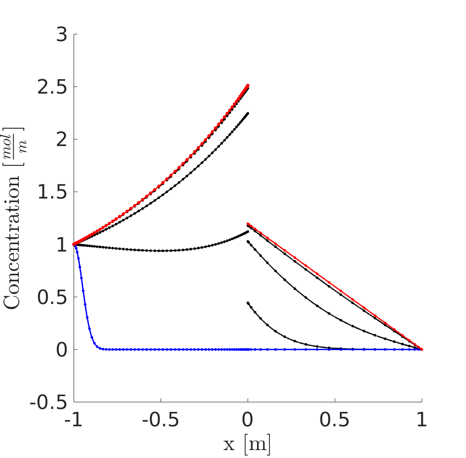
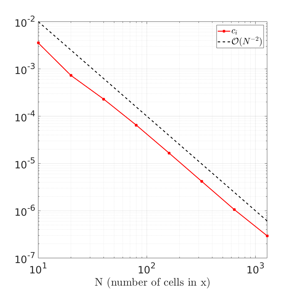
Figure 7: Left: Molar concentration results of $c_{\text{f}}$ in fluid (dashed for pnpMultiFoam, markers for Chebfun) and $c_{\text{s}}$ in solid (solid for pnpMultiFoam, markers for Chebfun). Blue for initial concentrations, black at intermediate times, red for final time (i.e steady state), Right: $L^{2}$ norm convergence plot between Chebfun and mappedChemicalKinetics/pnpMultiFoam

6.4 Random porous REV

To demonstrate the capabilities of our solvers, we consider a randomly generated porous solid-fluid domain $\Omega=\Omega_{\text{s}}\cup\Omega_{\text{f}}$, see fig. 8. The random generation is done by a truncated Gaussian random field [12, 24], sampled at the mesh points and categorized into two bins, denoting solid and fluid cells, by a threshold. Raising or lowering this threshold alters the porosity of the domain.

To have $\Omega$ be a microscopic representative elementary volume (REV) of a much larger macroscopic porous medium, we apply periodic conditions along the outer boundaries $\Gamma_{\text{ext}}=\Gamma_{\text{in}}\cup\Gamma_{\text{out}}\cup\Gamma_{\text{t}}\cup\Gamma_{\text{b}}$. To generate movement, we fix a jump in $\phi$ between $\Gamma_{\text{in,s}}$ and $\Gamma_{\text{out,s}}$, where the subscript $s$ denotes the section of $\Gamma_{\text{in}}$ neighbouring $\Omega_{\text{s}}$. This is to mimic a fixed applied potential difference across the macroscopic medium, such as an applied voltage across a battery cell. We consider two ion species $c_{1}$ and $c_{2}$ with opposite valencies $z_{1}=-z_{2}=-1$. The height and length of the region is set as $H=1\times 10^{-4}$m.

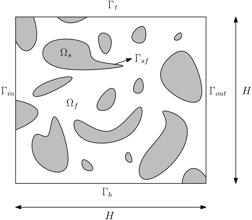
Figure 8: Visual representation of the random porous domain containing solid $\Omega_{\text{s}}$ (grey) and fluid $\Omega_{\text{f}}$ (white) with shared interface $\Gamma_{\text{sf}}$.

In $\Omega_{\text{f}}$ we start with a uniform concentration of $c_{2}$, the same is done for $\Omega_{\text{s}}$ with $c_{1}$. Fluid is initially taken at rest. Along $\Gamma_{\text{sf}}$ we set no flux for $c_{1}$ and flux continuity for $c_{2}$. For $\phi$ we assume continuity of the electric displacement $\mathbf{D}=\varepsilon\mathbf{E}$ along $\Gamma_{\text{sf}}$. In Table 4 we list the dimensionless number values of the case.

Symbol	$\mathcal{N}$	Pe	$\mathcal{L}$	$\mathcal{P}$
Value	$0.4$	$9.65\times 10^{-4}$	$0.95$	$1$

Table 4: Dimensionless numbers for the random porous media testcase.

The system is initialized with constant $c_{1}$ and $c_{2}$ in $\Omega_{\text{f}}$ and $\Omega_{\text{s}}$ respectively. All fields are periodic on the outer boundaries $\Gamma_{\text{ext}}=\Gamma_{\text{in}}\cup\Gamma_{\text{out}}\cup\Gamma_{\text{t}}\cup\Gamma_{\text{b}}$, apart from $\phi$ where we introduce a quasi-periodic condition with a fixed jump between $\Gamma_{\text{in,s}}$ and $\Gamma_{\text{out,s}}$, denoting the parts of $\Gamma_{\text{in}}$ and $\Gamma_{\text{out}}$ neighbouring $\Omega_{\text{s}}$. We apply no flux and flux continuity for $c_{1}$ and $c_{\text{s}}$ along $\Gamma_{\text{sf}}$ respectively. For $\phi$ we assume continuity of the electric displacement $\mathbf{D}=\varepsilon\mathbf{E}$ along $\Gamma_{\text{sf}}$:

$$c_{1}(\mathbf{x},0)=0\,,\quad c_{2}(\mathbf{x},0)=1\times 10^{-8}\,,\quad\phi(\mathbf{x},0)=0,\quad \mathbf{x}\in\Omega_{\text{s}};$$ (85)

$$c_{1}(\mathbf{x},0)=1\times 10^{-8}\,,\quad c_{2}(\mathbf{x},0)=0\,,\quad\phi(\mathbf{x},0)=0\,,\quad\mathbf{u}(\mathbf{x},0)=\mathbf{0}\,,\quad p(\mathbf{x},0)=0,\quad \mathbf{x}\in\Omega_{\text{f}};$$ (86)

$$\bigg{[}\bm{\nabla}_{\mathbf{n}}a\bigg{]}^{\Gamma_{\text{in,s}}}_{\Gamma_{\text{out,s}}}=0\,,\quad\bigg{[}a\bigg{]}^{\Gamma_{\text{in,s}}}_{\Gamma_{\text{out,s}}}=0\,,\quad\bigg{[}\bm{\nabla}_{\mathbf{n}}\phi\bigg{]}^{\Gamma_{\text{in,s}}}_{\Gamma_{\text{out,s}}}=0\,,\quad\bigg{[}\phi\bigg{]}^{\Gamma_{\text{in,s}}}_{\Gamma_{\text{out,s}}}=1\times 10^{-2},\quad a\in\{c_{1},c_{2}\};$$ (87)

$$\bigg{[}\bm{\nabla}_{\mathbf{n}}a\bigg{]}^{\Gamma_{\text{in,f}}}_{\Gamma_{out,f}}=0\,,\quad\bigg{[}a\bigg{]}^{\Gamma_{\text{in,f}}}_{\Gamma_{out,f}}=0,\quad a\in\{c_{1},c_{2},\phi,p,\mathbf{u}\};$$ (88)

$$\bigg{[}\bm{\nabla}_{\mathbf{n}}a\bigg{]}^{\Gamma_{\text{t}}}_{\Gamma_{\text{b}}}=0\,,\quad\bigg{[}a\bigg{]}^{\Gamma_{\text{t}}}_{\Gamma_{\text{b}}}=0,\quad a\in\{c_{1},c_{2},\phi,p,\mathbf{u}\};$$ (89)

$$\mathbf{j}_{1}\cdot\mathbf{n}=0\,,\quad\bigg{[}\mathbf{j}_{2}\cdot\mathbf{n}\bigg{]}^{\Gamma_{\text{sf,f}}}_{\Gamma_{\text{sf,s}}}=0\,,\quad\bm{\nabla}p\cdot\mathbf{n}=0\,,\quad\mathbf{u}\cdot\mathbf{n}=0\,,\quad\bigg{[}\varepsilon\bm{\nabla}_{\mathbf{n}}\phi\bigg{]}^{\Gamma_{\text{sf,f}}}_{\Gamma_{\text{sf,s}}}=0,\quad \mathbf{x}\in\Gamma_{\text{sf}}.$$ (90)

To show consistency in the results we run four simulations in total. This is done for two randomly generated meshes, each discretized over two levels of refinement for $N=1\times 10^{4}$ and $N=4\times 10^{4}$ cells. We will use letters $A$ and $B$ to differentiate between the random generations and subscripts $1$ and $2$ for the levels of refinement. E.g., $A_{2}$ denotes the first random mesh, refined using $4\times 10^{4}$ cells. All runs use a time step $\Delta t=5\times 10^{-4}$ and second-order implicit time scheme backwards. To observe the advective and electrostatic effects on our ions we define the following velocities in $\Omega_{\text{f}}$:

$$\mathbf{v}_{i}=\mathbf{u}-\frac{D_{i}z_{i}F}{RT}\bm{\nabla}\phi,$$ (91)

such that the continuity eq. 6 in $\Omega_{\text{f}}$ may be written as

$$\frac{\partial c_{i}}{\partial t}+\bm{\nabla}\cdot\left(\mathbf{v}_{i}c_{i}-D_{i}\bm{\nabla}c_{i}\right)=0.$$ (92)

Figure 9 shows the results of the first random realization with a finer mesh ($N=4\times 10^{4}$), where we observe a gradient in $\phi$ formed between regions of $\Omega_{\text{s}}$ connected at $\Gamma_{\text{in}}$ and $\Gamma_{\text{out}}$. This is primarily due to our jump condition for $\phi$ applied along $\Gamma_{\text{in,s}}$ and $\Gamma_{\text{out,s}}$. Whilst the movement of our ion species has an effect on this gradient, for the most part, it remains steady. The applied electrical driving force causes the uniform concentration $c_{1}$ in $\Omega_{\text{f}}$ to accumulate around the regions of $\Omega_{\text{s}}$ connected at $\Gamma_{\text{out}}$, where a higher electric potential is present. Conversely, around $\Omega_{\text{s}}$ connected at $\Gamma_{\text{in}}$ we find a much lower, but not zero, concentration of $c_{1}$. A similar observation is found with $c_{2}$, once diffused out of $\Omega_{\text{s}}$, accumulating where there is a lower potential. As with $c_{1}$, at the region of $\Omega_{\text{s}}$ connected at $\Gamma_{\text{out}}$ there is a much lower, but again not zero, concentration of $c_{2}$. We observe therefore the formation of EDLs, see §3, around these connected solids. Given more time to evolve these EDLs would become further apparent, with more of $c_{2}$ diffusing out of $\Omega_{\text{s}}$. As for $\mathbf{v}_{1}$ and $\mathbf{v}_{2}$ we find their magnitudes $||\mathbf{v}_{1}||$ and $||\mathbf{v}_{2}||$ are highest within these EDLs located at the connected solids due to higher gradients in $\phi$.

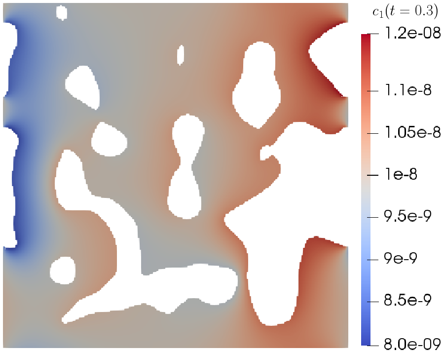
(a)

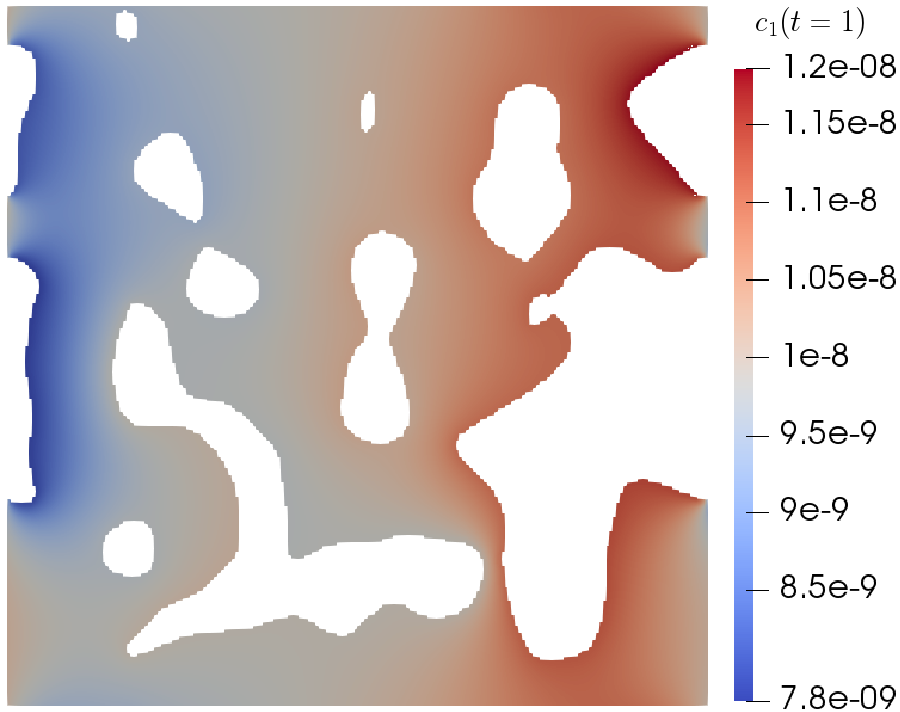
(b)

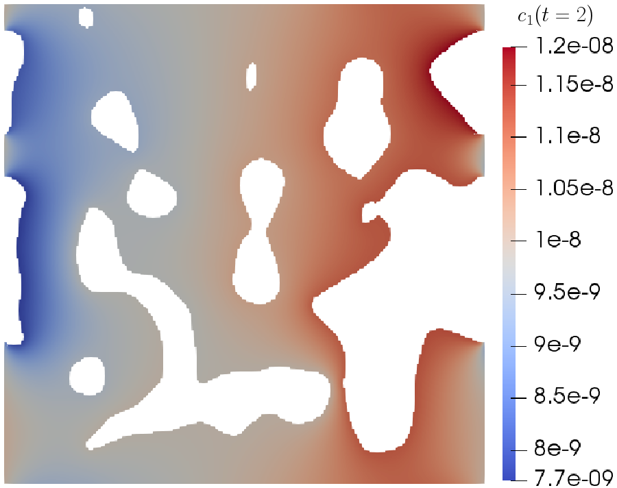
(c)

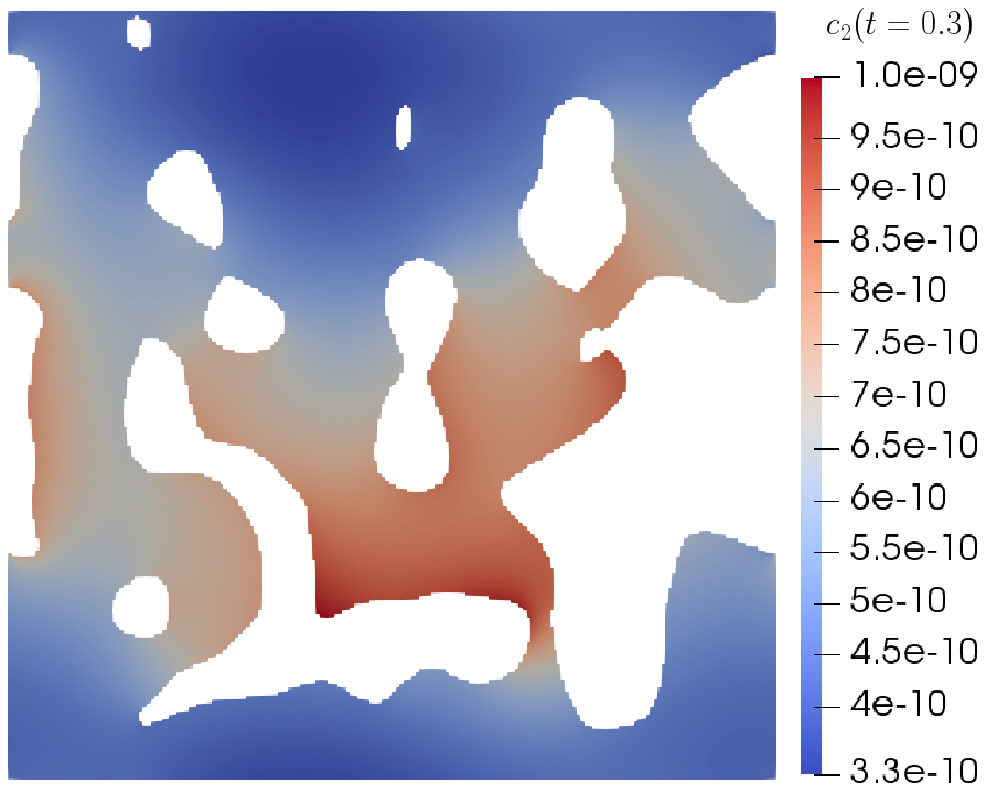
(d)

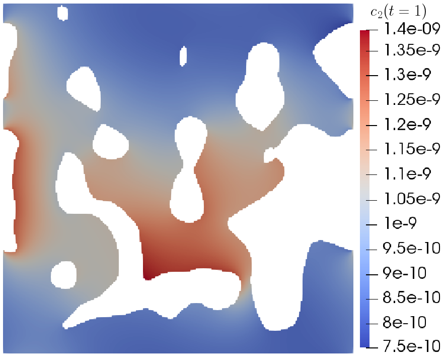
(e)

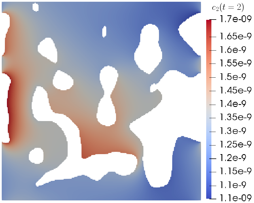
(f)

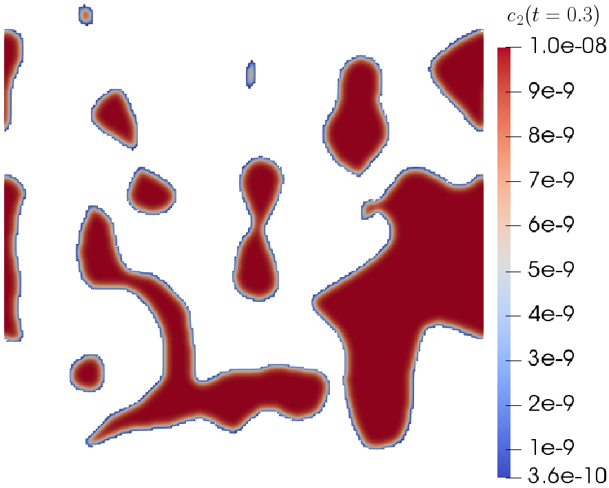
(g)

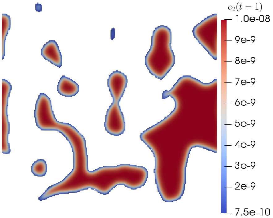
(h)

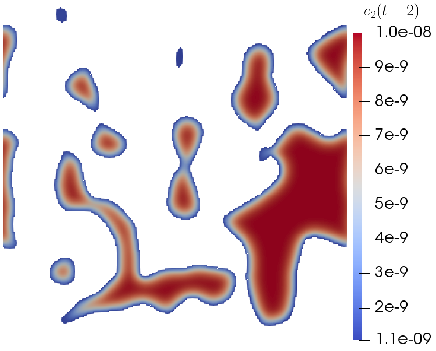
(i)

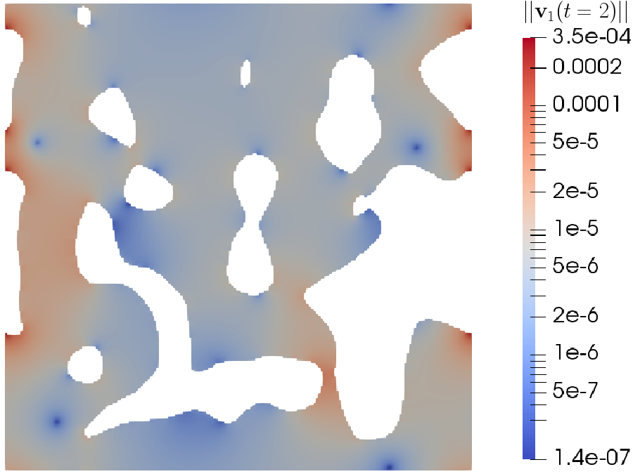
(j)

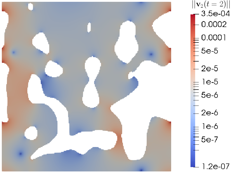
(k)

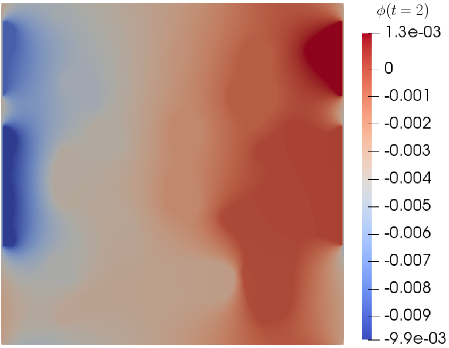
(l)

Figure 9: Results of the first random solid-fluid geometry, discretized using $4\times 10^{4}$ cells. (a)-(f): Profiles of $c_{1}$ and $c_{2}$ at $t=0.3$, $1$, $2$s within $\Omega_{\text{f}}$. (g)-(i): Profiles of $c_{2}$ at $t=0.3$, $1$, $2$s within $\Omega_{\text{s}}$. (j)-(l): Profiles of $||\mathbf{v}_{1}||$, $||\mathbf{v}_{2}||$ and $\phi$ at $t=2$s.

We can compare these results with coarse mesh ($N=1\times 10^{4}$) results as well as with other random generation seeds. Results of the first realization with a coarse mesh, and of a coarse and fine simulation of a second random realization are reported respectively in fig. 10, fig. 11, and fig. 12.

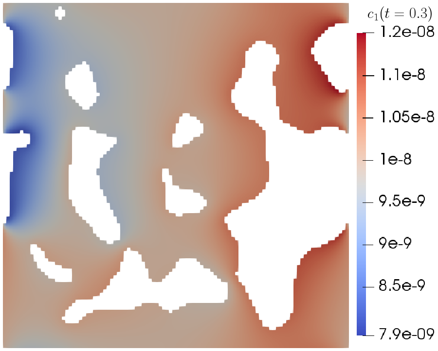
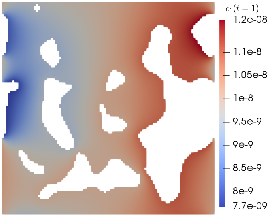
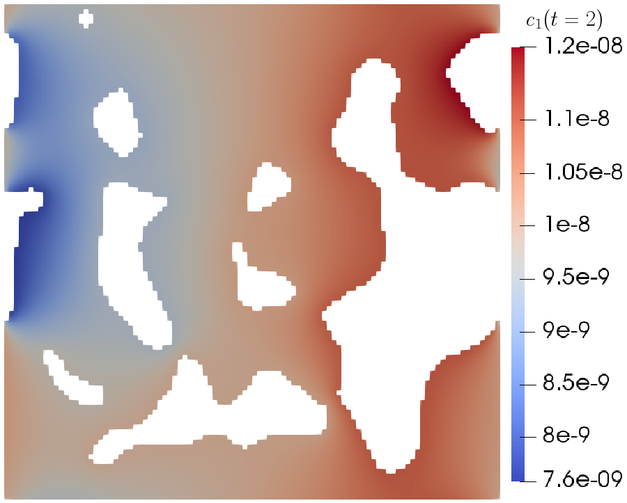
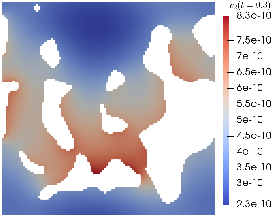
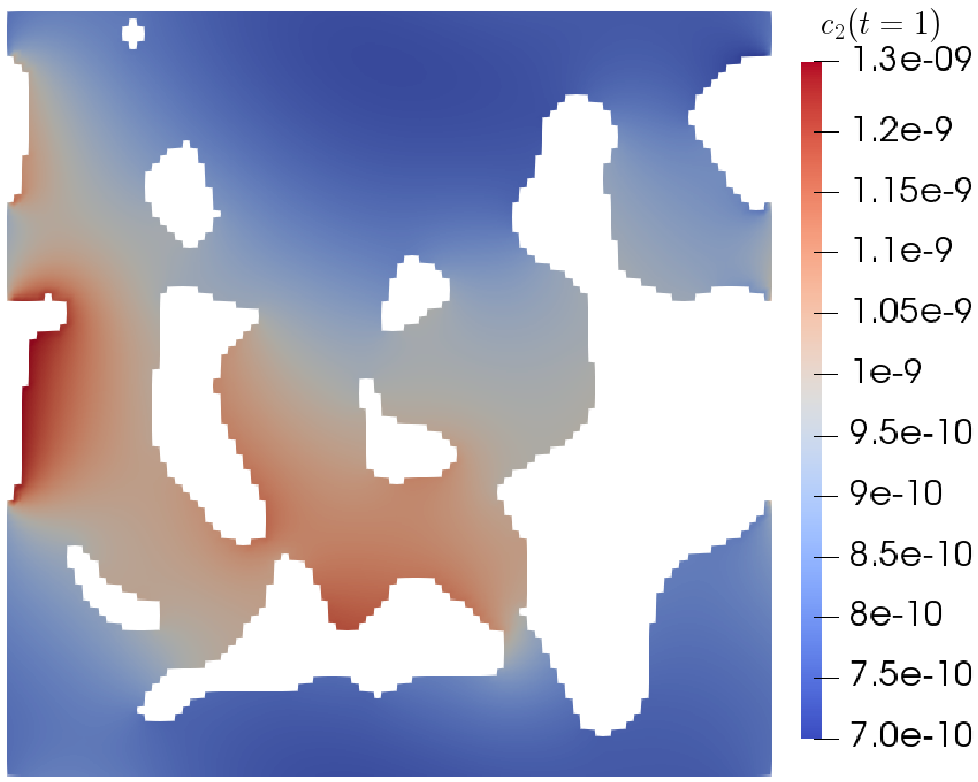
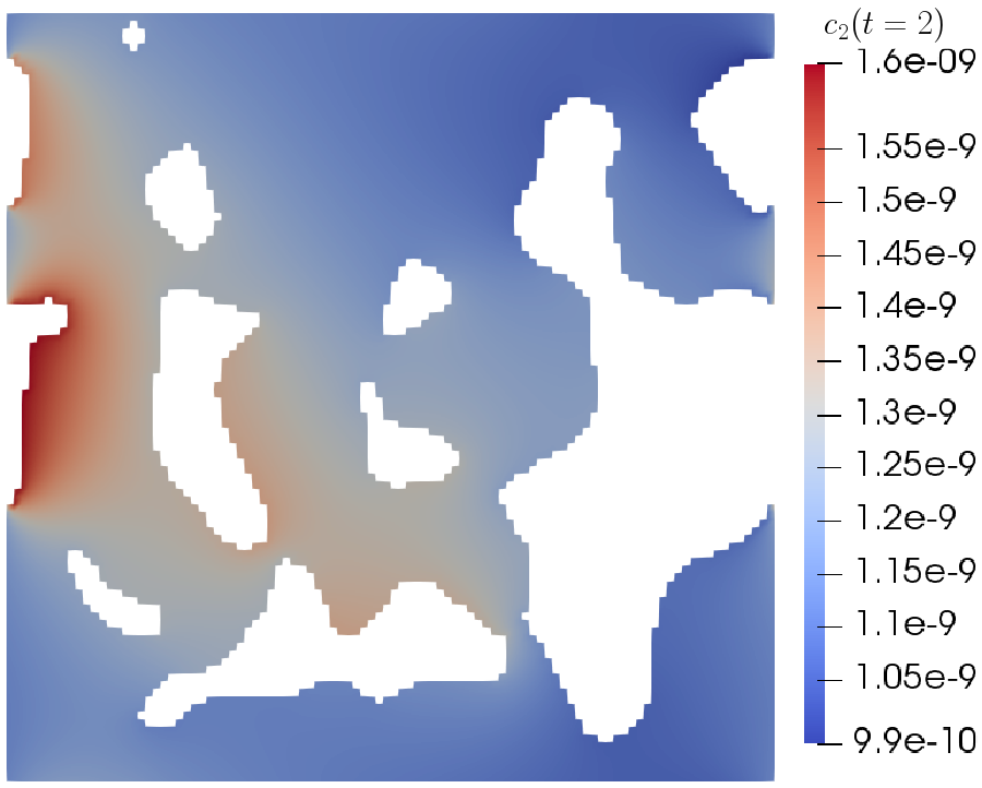
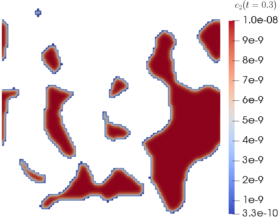
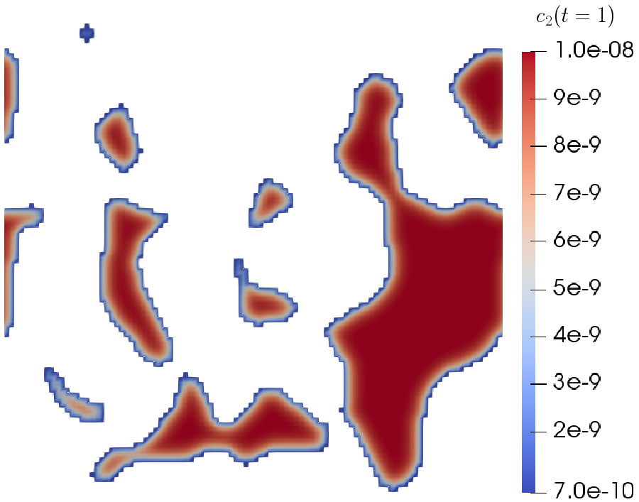
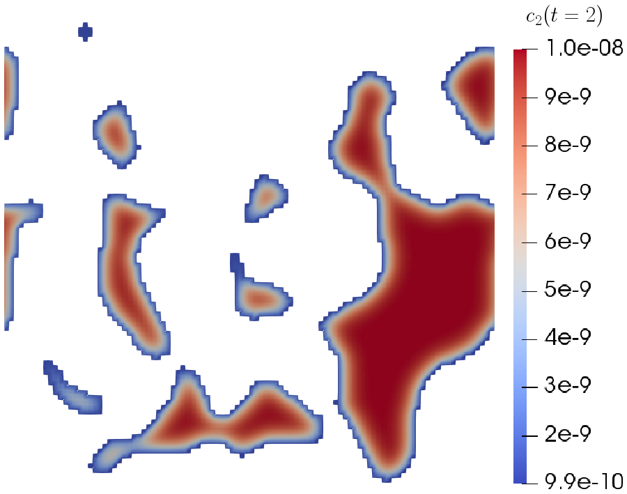
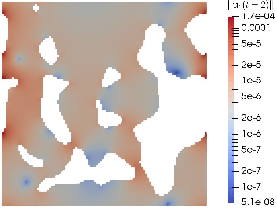
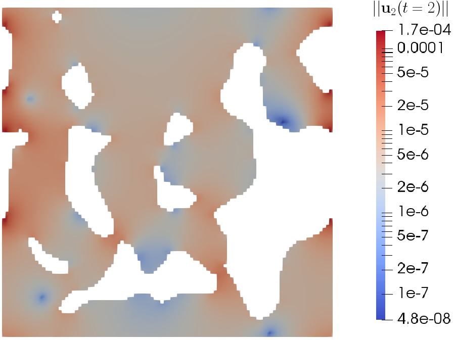
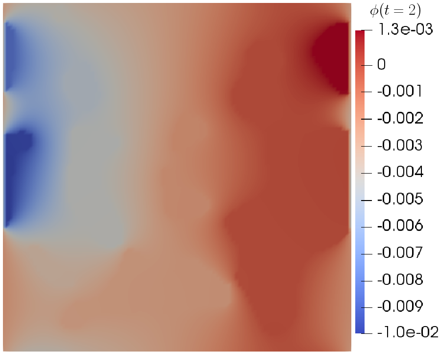
Figure 10: Results of the first random solid-fluid geometry, discretized using $N=1\times 10^{4}$ cells. Top two rows: Profiles of $c_{1}$ and $c_{2}$ at $t=0.3$, $1$, $2$s within $\Omega_{\text{f}}$. Third row: Profiles of $c_{2}$ at $t=0.3$, $1$, $2$s within $\Omega_{\text{s}}$. Bottom row: Profiles of $||\mathbf{u}_{1}||$, $||\mathbf{u}_{2}||$ and $\phi$ at $t=2$s.

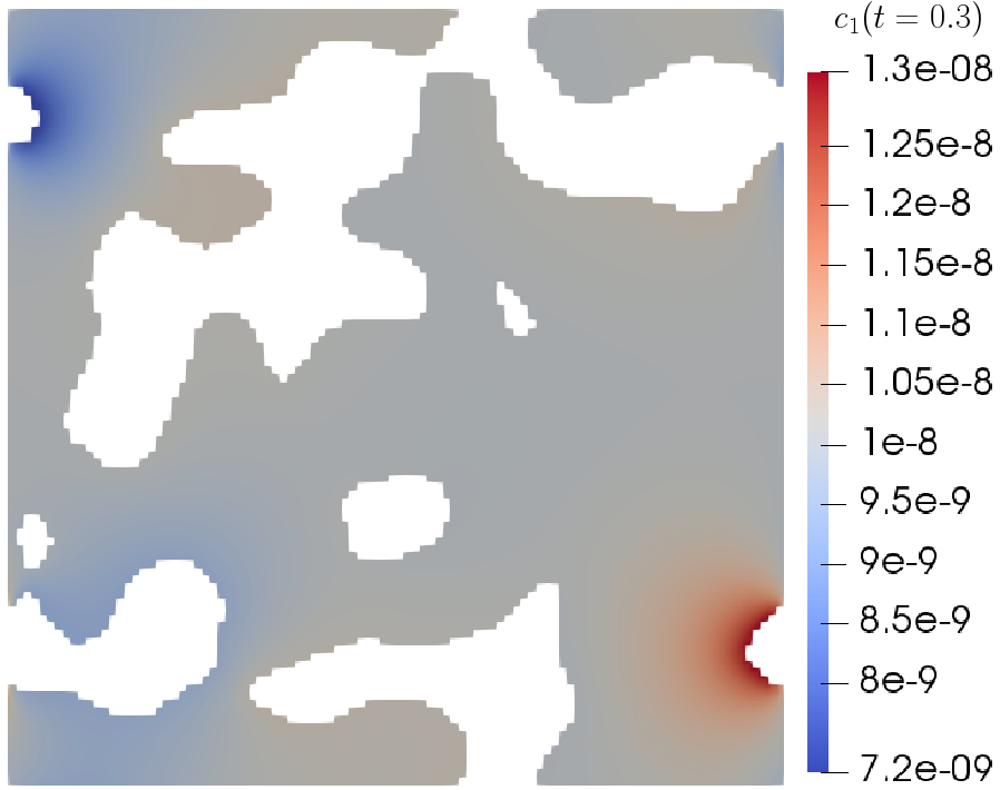
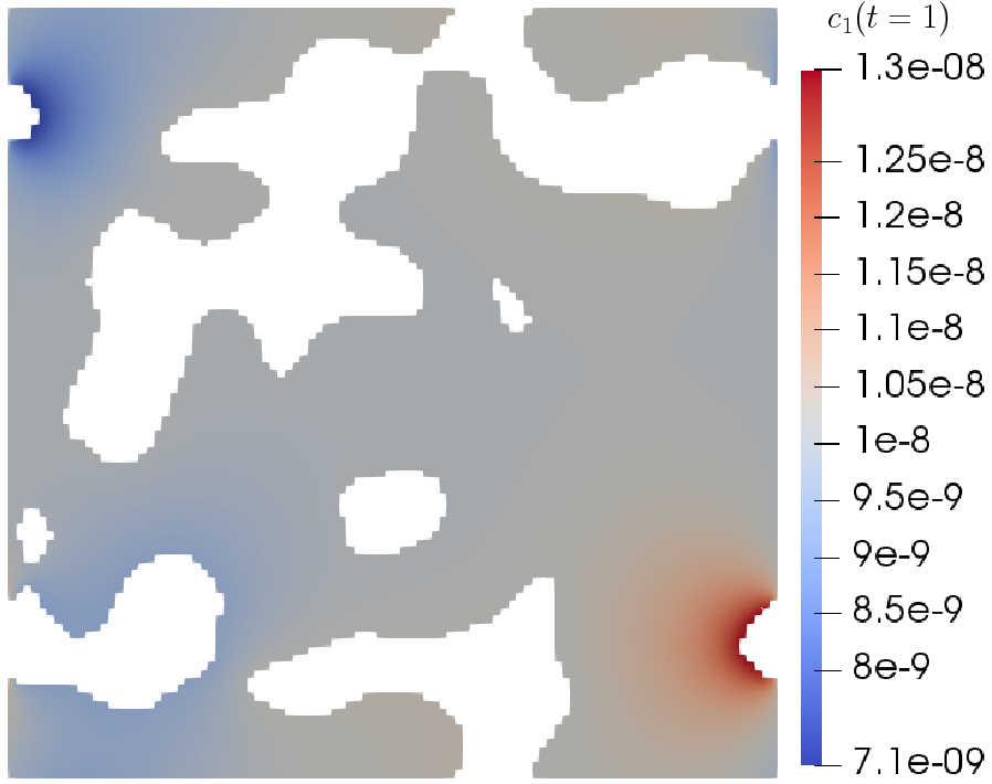
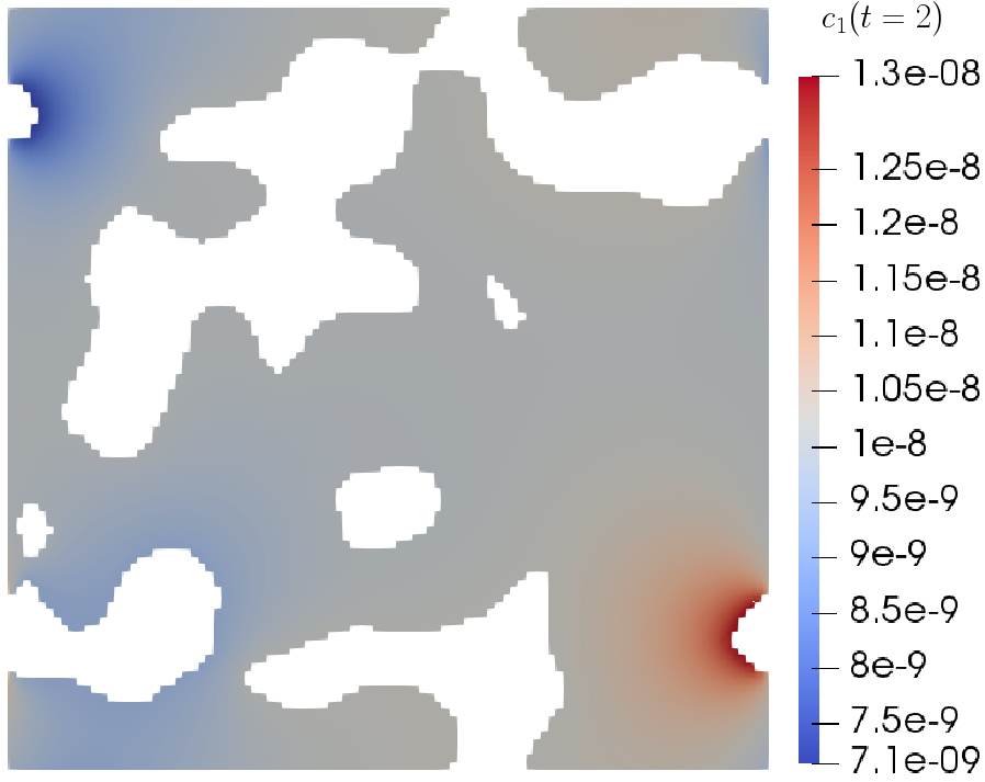
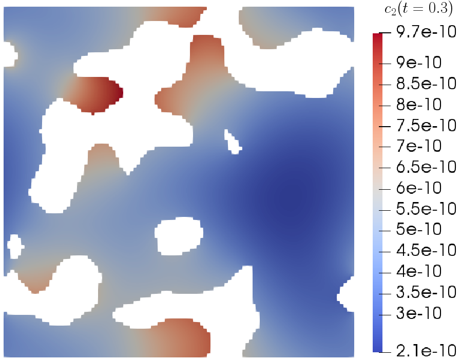
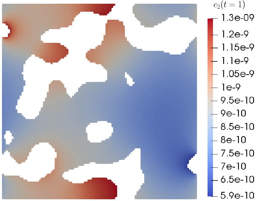
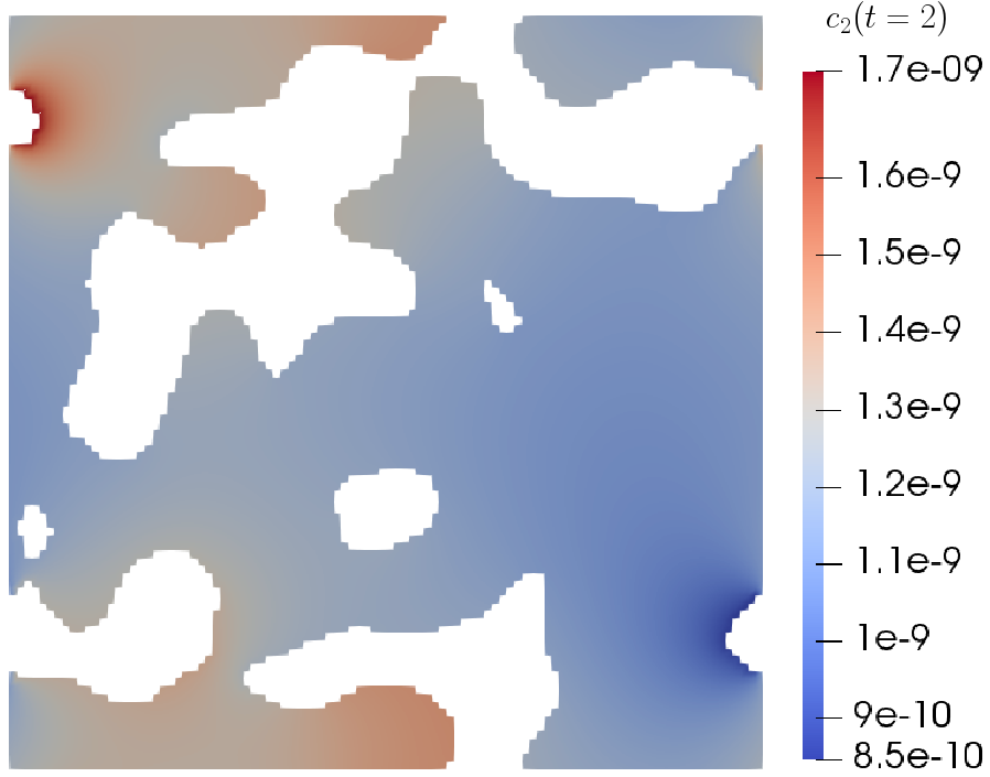
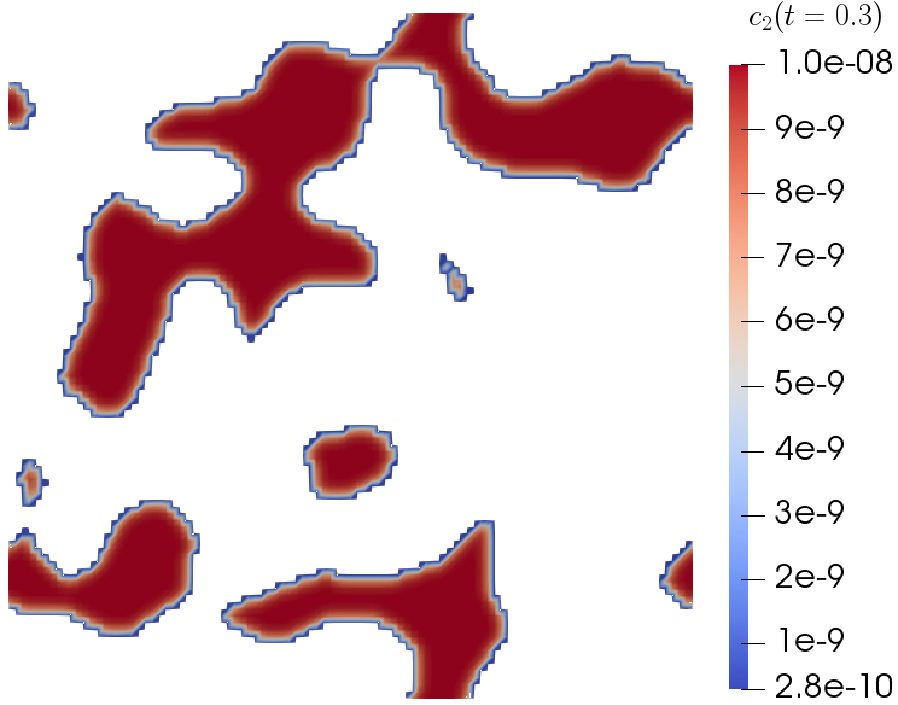
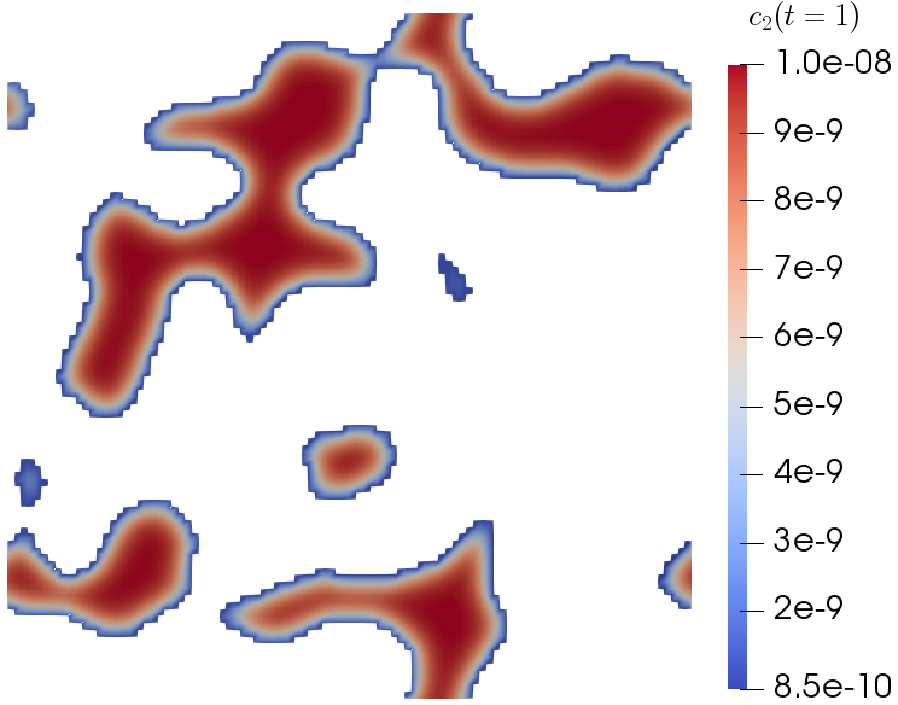
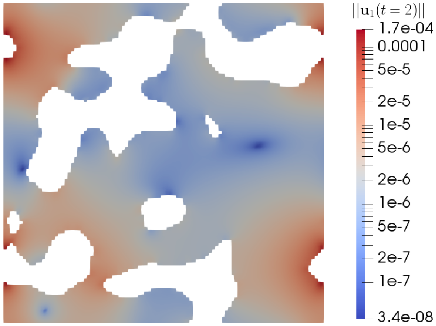
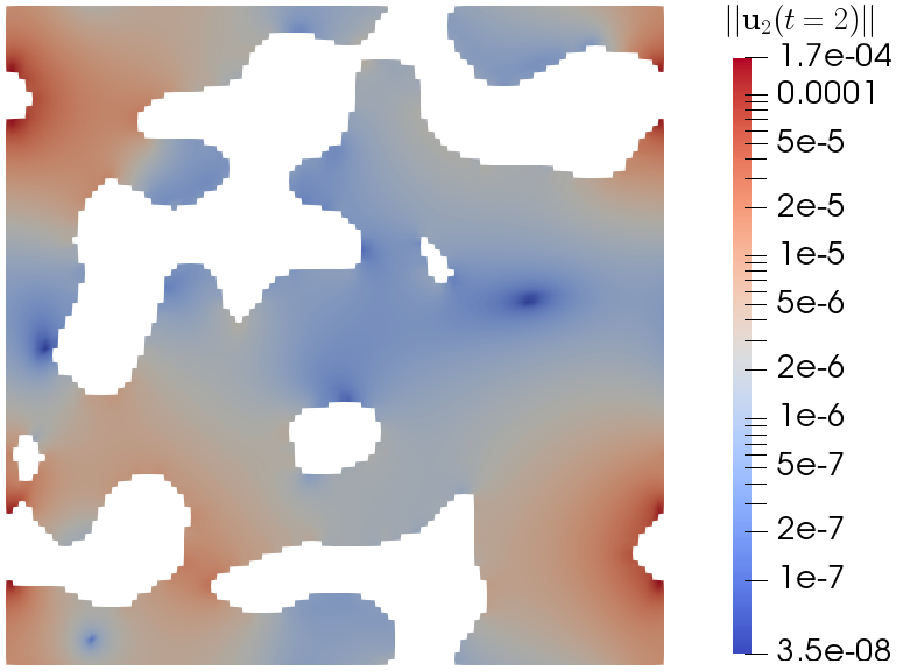
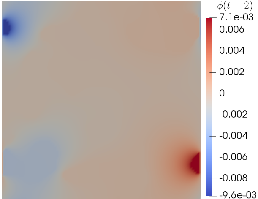
Figure 11: Results of the second random solid-fluid geometry, discretized using $N=1\times 10^{4}$ cells. Top two rows: Profiles of $c_{1}$ and $c_{2}$ at $t=0.3$, $1$, $2$s within $\Omega_{\text{f}}$. Third row: Profiles of $c_{2}$ at $t=0.3$, $1$, $2$s within $\Omega_{\text{s}}$. Bottom row: Profiles of $||\mathbf{u}_{1}||$, $||\mathbf{u}_{2}||$ and $\phi$ at $t=2$s.

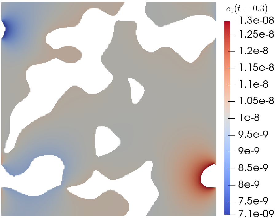
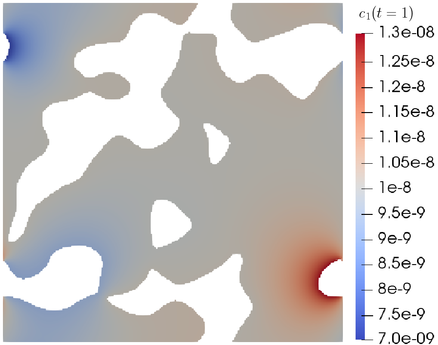
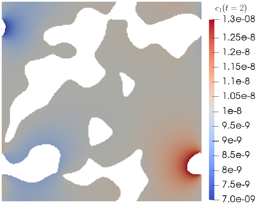
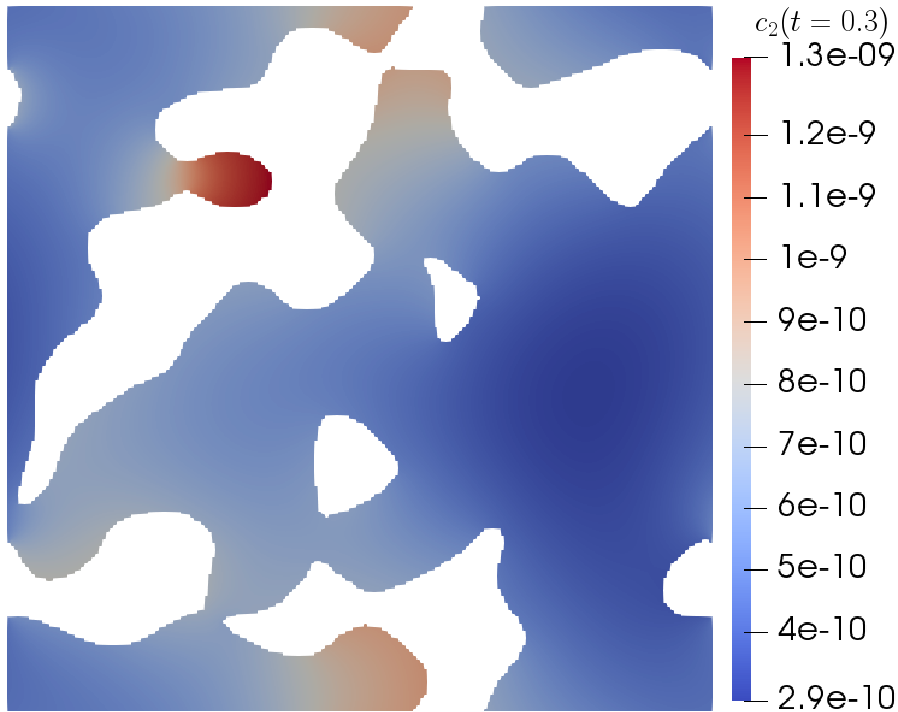
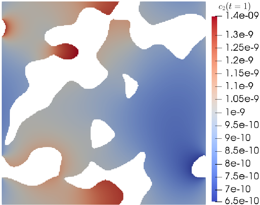
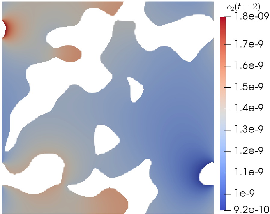
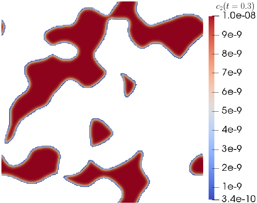
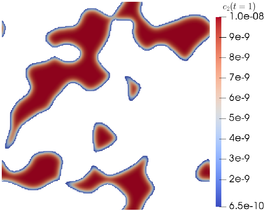
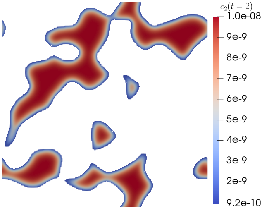
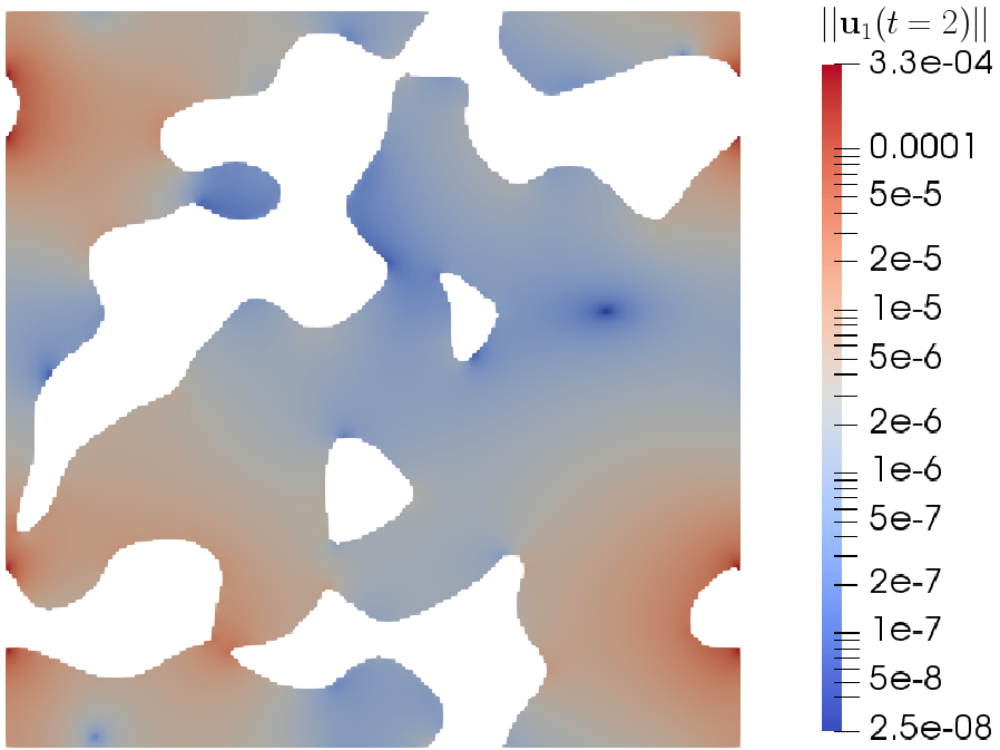
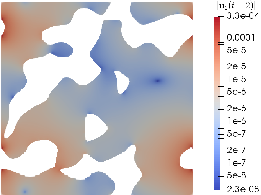
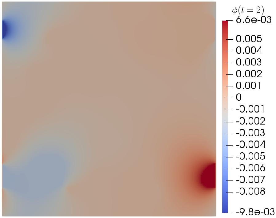
Figure 12: Results of the second random solid-fluid geometry, discretized using $N=4\times 10^{4}$ cells. Top two rows: Profiles of $c_{1}$ and $c_{2}$ at $t=0.3$, $1$, $2$s within $\Omega_{\text{f}}$. Third row: Profiles of $c_{2}$ at $t=0.3$, $1$, $2$s within $\Omega_{\text{s}}$. Bottom row: Profiles of $||\mathbf{u}_{1}||$, $||\mathbf{u}_{2}||$ and $\phi$ at $t=2$s.

7 Conclusions

In this paper, we present the development of open-source solvers in OpenFOAM^® capable of simulating microscopic electrokinetic flows of dilute ionic fluids. The underlying system, known as Stokes-Poisson-Nernst-Planck, is thoroughly reviewed where we discuss the assumptions on the fluid properties and limitations these bring. We later apply dimensional analysis to characterize the effects of dominating physical forces. This analysis is later used to give a better understanding of a common model reduction, known as the electro-neutrality assumption, as a result of such analysis.

Many real-world applications of these flows involve some form of reactions between involved ionic species at the interface between fluid and solid. As such, we formulate a fully general reaction model capable of describing said heterogeneous reactions as a balance of fluxes across all reacting species.

To verify flow descriptions obtained from our solvers are accurate, we compare against highly accurate solutions obtained, for simplified cases, with the Matlab toolbox Chebfun for a number of cases. With each case we find good agreement, showing spatial grid convergence of the results. We later use our solvers across a randomly generated solid-fluid porous cell, similar to a representative elementary volume (REV) used in homogenization theory, to show the solver’s ability in handling complex microstructures.

In future works, we plan on constructing fully physically realistic cases, such as modelling the electrokinetic flow through a porous battery half-cell. Furthermore, we later plan to apply uncertainty quantification in conjunction with these randomly generated porous cells, quantifying the effects on the flow for varying geometrical properties.

Declarations

The authors declare that they have no conflicts of interest. MI and RB have been supported by the University of Nottingham Impact Acceleration Award.

Appendix A Quasi-coupled Newton iterative effective reactive Robin conditions

A.1 General non-linear reaction rate for restricted binary reaction

Let there be the following reversible binary reaction between species $c_{\text{s}}$ and $c_{\text{f}}$ along the interface $\Gamma$ shared by $\Omega_{\text{s}}$ and $\Omega_{\text{f}}$,

$$\ce{\nu_{\text{s}}X_{\text{s}}<=>\nu_{\text{f}}X_{\text{f}}},$$ (93)

and consider each species restricted to its respective sub-domains:

$$c_{\text{s}}=\begin{cases}0&\mathbf{x}\in\Omega_{\text{f}}\\ c_{\text{s}}&\mathbf{x}\in\Omega_{\text{s}}\end{cases},\qquad c_{\text{f}}=\begin{cases}c_{\text{f}}&\mathbf{x}\in\Omega_{\text{f}}\\ 0&\mathbf{x}\in\Omega_{\text{s}}\end{cases}.$$ (94)

In these circumstances, we have the following condition along $\Gamma$ with reaction rate $r$:

$$\mathbf{j}_{\text{s}}\big{\rvert}_{\Gamma_{\text{s}}}\cdot\mathbf{n}=r(c_{\text{s}}\rvert_{\Gamma_{\text{s}}},c_{\text{f}}\rvert_{\Gamma_{\text{f}}})=-\mathbf{j}_{\text{f}}\big{\rvert}_{\Gamma_{\text{f}}}\cdot\mathbf{n^{\prime}}.$$ (95)

We denote here $\mathbf{n}$ to be the unit normal along $\Gamma$ facing outwards of $\Omega_{\text{s}}$ and $\mathbf{n^{\prime}}=-\mathbf{n}$. Consider the reaction rate $r$ is a non-linear function of $c_{\text{s}}$ and $c_{\text{f}}$. To obtain effective Robin conditions of eq. 95 for $c_{\text{s}}$ and $c_{\text{f}}$ we employ the Newton-Raphson method. First, we take the vector form of eq. 95 with all terms moved to the left. To simplify writing, for now we omit what side of $\Gamma$ each term is evaluated on:

$$\mathbf{J}(c_{\text{s}},c_{\text{f}})=\begin{pmatrix}J_{1}\\ J_{2}\end{pmatrix}\equiv\begin{pmatrix}-D_{\text{s}}\bm{\nabla}_{\mathbf{n}}c_{\text{s}}-r(c_{\text{s}},c_{\text{f}})\\[6.0pt] (\mathbf{u}_{\text{f}}\cdot\mathbf{n}^{\prime})c_{\text{f}}-D_{\text{f}}\bm{\nabla}_{\mathbf{n}^{\prime}}c_{\text{f}}-\frac{z_{\text{f}}D_{\text{f}}F}{RT}c_{\text{f}}\bm{\nabla}_{\mathbf{n}^{\prime}}\phi_{\text{f}}+r(c_{\text{s}},c_{\text{f}})\end{pmatrix}=\mathbf{0}.$$ (96)

Assume we have a current approximate solution $\mathbf{c}^{N}=(c_{\text{s}}^{N}\hskip 5.0ptc_{\text{f}}^{N})^{\top}$. Linearizing $\mathbf{J}$ around $\mathbf{c}^{N}$ then gives

$$\mathbf{J}(\mathbf{c}^{N})+\frac{\partial\mathbf{J}}{\partial\mathbf{c}}\bigg{\rvert}_{\mathbf{c}^{N}}\left(\mathbf{c}-\mathbf{c}^{N}\right)=\mathbf{0},$$ (97)

whereby setting $\mathbf{c}=\mathbf{c}^{N+1}$ is the next iterative solution. We denote here $\frac{\partial\mathbf{J}}{\partial\mathbf{c}}$ to be the Jacobian matrix of $\mathbf{J}$. To determine the Jacobian we define the directional derivative for some function $G(c)$ along the direction $\delta c=c-c^{N}$ as:

$$\frac{\partial G}{\partial c}(\delta c)=\lim_{\varepsilon\rightarrow 0}\frac{G(c+\varepsilon\delta c)-G(c)}{\varepsilon}.$$ (98)

Using this definition of the directional derivative we can then determine the Jacobian within eq. 97. Since the method is similar for all components of $\mathbf{J}$, we will focus on the first element $J_{1}$. Taking the directional derivative of $J_{1}$ with respect to $c_{\text{s}}$ along $\delta c_{\text{s}}$ at $\mathbf{c}=\mathbf{c}^{N}$ gives:

$$\frac{\partial J_{1}}{\partial c_{\text{s}}}\bigg{\rvert}_{\mathbf{c}^{N}}(\delta c_{\text{s}})=\lim_{\varepsilon\rightarrow 0}\frac{1}{\varepsilon}\left(-D_{\text{s}}\bm{\nabla}_{\mathbf{n}}(c_{\text{s}}^{N}+\varepsilon\delta c_{\text{s}})-r(c_{\text{s}}^{N}+\varepsilon\delta c_{\text{s}},c_{\text{f}}^{N})+D_{\text{s}}\bm{\nabla}_{\mathbf{n}}c_{\text{s}}^{N}+r(c_{\text{s}}^{N},c_{\text{f}}^{N})\right).$$ (99)

Taking the following Taylor expansions about $\varepsilon=0$ of $r$ and the concentration gradient,

$$\bm{\nabla}_{\mathbf{n}}(c_{\text{s}}^{N}+\varepsilon\delta c_{\text{s}}) =\bm{\nabla}_{\mathbf{n}}c_{\text{s}}^{N}+\varepsilon\bm{\nabla}_{\mathbf{n}}\delta c_{\text{s}}+\mathcal{O}(\varepsilon^{2}),$$ (100)

$$r(c_{\text{s}}^{N}+\varepsilon\delta c_{\text{s}},c_{\text{f}}^{N}) =r(c_{\text{s}}^{N},c_{\text{f}}^{N})+\varepsilon\delta c_{\text{s}}\frac{\partial r}{\partial c_{\text{s}}}\bigg{\rvert}_{\mathbf{c}^{N}}+\mathcal{O}(\varepsilon^{2}),$$ (101)

then substituting into eq. 99 we obtain:

$$\frac{\partial J_{1}}{\partial c_{\text{s}}}\bigg{\rvert}_{\mathbf{c}^{N}}(\delta c_{\text{s}})=-D_{\text{s}}\bm{\nabla}_{\mathbf{n}}\delta c_{\text{s}}-\delta c_{\text{s}}\frac{\partial r}{\partial c_{\text{s}}}\bigg{\rvert}_{\mathbf{c}^{N}}.$$ (102)

The same can be done to find the directional derivative of $J_{1}$ with respect to $c_{\text{f}}$, giving:

$$\frac{\partial J_{1}}{\partial c_{\text{f}}}\bigg{\rvert}_{\mathbf{c}^{N}}(\delta c_{\text{f}})=-\delta c_{\text{f}}\frac{\partial r}{\partial c_{\text{f}}}\bigg{\rvert}_{\mathbf{c}^{N}}.$$ (103)

Repeating the same process for $J_{2}$ of eq. 96 and collecting all elements together and evaluating at $\mathbf{c}^{N}$ gives

$$\frac{\partial\mathbf{J}}{\partial\mathbf{c}}\bigg{\rvert}_{\mathbf{c}^{N}}\left(\mathbf{\delta c}\right)=\begin{pmatrix}-D_{\text{s}}\bm{\nabla}_{\mathbf{n}}\delta c_{\text{s}}-\delta c_{\text{s}}\frac{\partial r}{\partial c_{\text{s}}}-\delta c_{\text{f}}\frac{\partial r}{\partial c_{\text{f}}}\\[6.0pt] \delta c_{\text{s}}\frac{\partial r}{\partial c_{\text{s}}}+(\mathbf{u}_{\text{f}}\cdot\mathbf{n}^{\prime})\delta c_{\text{f}}-\frac{z_{\text{f}}D_{\text{f}}F}{RT}\delta c_{\text{f}}\bm{\nabla}_{\mathbf{n}}\phi_{\text{f}}+\delta c_{\text{f}}\frac{\partial r}{\partial c_{\text{f}}}\end{pmatrix},$$ (104)

where derivatives in $r$ are evaluated at $\mathbf{c}^{N}$. We may then substitute eq. 104 into eq. 97 to get

$$\begin{pmatrix}-D_{\text{s}}\bm{\nabla}_{\mathbf{n}}c_{\text{s}}-r-\delta c_{\text{f}}\frac{\partial r}{\partial c_{\text{f}}}-\delta c_{\text{s}}\frac{\partial r}{\partial c_{\text{s}}}\\[6.0pt] (\mathbf{u}_{\text{f}}\cdot\mathbf{n}^{\prime})c_{\text{f}}-D_{\text{f}}\bm{\nabla}_{\mathbf{n}^{\prime}}c_{\text{f}}-\frac{z_{\text{f}}D_{\text{f}}F}{RT}c_{\text{f}}\bm{\nabla}_{\mathbf{n}^{\prime}}\phi_{\text{f}}+r+\delta c_{\text{s}}\frac{\partial r}{\partial{c}_{\text{s}}}+\delta c_{\text{f,f}}\frac{\partial r}{\partial c_{\text{f}}}\end{pmatrix}=\mathbf{0},$$ (105)

where $r$ and its derivatives are evaluated at $\mathbf{c}^{N}$. Re-arranging the first element of eq. 105, using the first order approximation $\bm{\nabla}_{\mathbf{n}}c_{\text{s}}=B_{\text{s}}(c_{\text{s}}-c_{\text{s,c}})$ where $c_{\text{s,c}}$ is the value at the cell centre of cells sharing a face with $\Gamma$, and substituting into the second element then gives:

$$(\mathbf{u}_{\text{f}}\cdot\mathbf{n}^{\prime})c_{\text{f}}-D_{\text{f}}\bm{\nabla}_{\mathbf{n}^{\prime}}c_{\text{f}}-\frac{z_{\text{f}}D_{\text{f}}F}{RT}c_{\text{f}}\bm{\nabla}_{\mathbf{n}^{\prime}}\phi_{\text{f}}=-r-\delta c_{\text{f}}\frac{\partial r}{\partial c_{\text{f}}}+c_{\text{s}}^{N}\frac{\partial r}{\partial c_{\text{s}}}+P(c_{\text{f}}),$$ (106)

where

$$P(c_{\text{f}})=\frac{\partial r}{\partial c_{\text{s}}}\left(\frac{-D_{\text{s}}B_{\text{s}}c_{\text{s,c}}+r+\delta c_{\text{f}}\frac{\partial r}{\partial c_{\text{f}}}-c_{\text{s}}^{N}\frac{\partial r}{\partial c_{\text{s}}}}{D_{\text{s}}B_{\text{s}}+\frac{\partial r}{\partial c_{\text{s}}}}\right).$$ (107)

Setting $\mathbf{c}=\mathbf{c}^{N+1}$ to indicate the next iterative solution results in an iterative Robin condition of the form $-D_{\text{f}}^{*}\bm{\nabla}_{\mathbf{n}^{\prime}}c_{\text{f}}^{N+1}=-K_{\text{f}}^{*}c_{\text{f}}^{N+1}-F_{\text{f}}^{*}$, with effective coefficients dependent on the previous iteration $\mathbf{c}^{N}$:

$$D_{\text{f}}^{*} =D_{\text{f}},$$ (108)

$$K_{\text{f}}^{*} =-\frac{\frac{\partial r}{\partial c_{\text{s}}}\frac{\partial r}{\partial c_{\text{f}}}}{D_{\text{s}}B_{\text{s}}+\frac{\partial r}{\partial c_{\text{s}}}}+\frac{\partial r}{\partial c_{\text{f}}}-\frac{z_{\text{f}}D_{\text{f}}F}{RT}\bm{\nabla}_{\mathbf{n}^{\prime}}\phi_{\text{f}}+(\mathbf{u}_{\text{f}}\cdot\mathbf{n}^{\prime}),$$ (109)

$$F_{\text{f}}^{*} =r-c_{\text{f}}^{N}\frac{\partial r}{\partial c_{\text{f}}}-c_{\text{s}}^{N}\frac{\partial r}{\partial c_{\text{s}}}-\frac{\partial r}{\partial c_{\text{s}}}\left(\frac{-D_{\text{s}}B_{\text{s}}c_{\text{s,c}}+r-c_{\text{f}}^{N}\frac{\partial r}{\partial c_{\text{f}}}-c_{\text{s}}^{N}\frac{\partial r}{\partial c_{\text{s}}}}{D_{\text{s}}B_{\text{s}}+\frac{\partial r}{\partial c_{\text{s}}}}\right).$$ (110)

Remember, $r$ and its derivatives are evaluated at the previous iteration $\mathbf{c}^{N}$. Similar steps can also be applied to the accompanying iterative Robin condition for $c_{\text{s}}$ of the form $-D_{\text{s}}^{*}\bm{\nabla}_{\mathbf{n}}c_{\text{s}}^{N+1}=-K_{\text{s}}^{*}c_{\text{s}}^{N+1}-F_{\text{s}}^{*}$, with coefficients:

$$D_{\text{s}}^{*} =D_{\text{s}},$$ (111)

$$K_{\text{s}}^{*} =\frac{\frac{\partial r}{\partial c_{\text{s}}}\frac{\partial r}{\partial c_{\text{f}}}}{(\mathbf{u}_{\text{f}}\cdot\mathbf{n}^{\prime})-D_{\text{f}}B_{\text{f}}-\frac{z_{\text{f}}D_{\text{f}}F}{RT}\bm{\nabla}_{\mathbf{n}^{\prime}}\phi_{\text{f}}+\frac{\partial r}{\partial c_{\text{f}}}}-\frac{\partial r}{\partial c_{\text{s}}},$$ (112)

$$F_{\text{s}}^{*} =-r+c_{\text{f}}^{N}\frac{\partial r}{\partial c_{\text{f}}}+c_{\text{s}}^{N}\frac{\partial r}{\partial c_{\text{s}}}-\frac{\partial r}{\partial c_{\text{f}}}\left(\frac{-D_{\text{f}}B_{\text{f}}c_{\text{f,c}}-r+c_{\text{f}}^{N}\frac{\partial r}{\partial c_{\text{f}}}+c_{\text{s}}^{N}\frac{\partial r}{\partial c_{\text{s}}}}{(\mathbf{u}_{\text{f}}\cdot\mathbf{n}^{\prime})-D_{\text{f}}B_{\text{f}}-\frac{z_{\text{f}}D_{\text{f}}F}{RT}\bm{\nabla}_{\mathbf{n}^{\prime}}\phi_{\text{f}}+\frac{\partial r}{\partial c_{\text{f}}}}\right).$$ (113)

A.2 General non-linear unrestricted reaction rate

Here we will formulate a set of iterative Robin conditions required to solve the reactive conditions for unrestricted species and non-linear reactions. Consider a general non-linear reaction with $i=J,...,K$ reactants and $i=K+1,...,M$ products:

$$\sum_{i=J}^{K}\nu_{i}B_{i}+ne^{-}=\sum_{i=K+1}^{M}\nu_{i}B_{i}\,.$$ (114)

We model eq. 114 using the following conditions with general, possibly non-linear, reaction rates $r_{i}$:

$$\big{[}\mathbf{j}_{i}\cdot\mathbf{n}\big{]}^{\Gamma_{\text{s}}}_{\Gamma_{\text{f}}} =r_{i}(c_{J},c_{J+1},\dots,c_{M})\qquad \mathbf{x}\in\Gamma\text{ for }i=J,...,M,$$ (115)

$$\big{[}c_{i}\big{]}^{\Gamma_{\text{s}}}_{\Gamma_{\text{f}}} =0\qquad \mathbf{x}\in\Gamma\text{ for }i=J,...,M.$$ (116)

We begin by writing $\mathbf{j}_{i}$ in full and use $\mathbf{n}=-\mathbf{n}^{\prime}$ to give $\mathbf{j}_{i}\rvert_{\Gamma_{\text{f}}}\cdot\mathbf{n}=-\mathbf{j}_{i}\rvert_{\Gamma_{\text{f}}}\cdot\mathbf{n}^{\prime}$, a more acceptable form for OpenFOAM^® . Since formulating the necessary Robin conditions is the same for all species $i$, we omit the subscript from here onward unless necessary. Instead, we introduce two new subscripts $s$ and $f$ denoting evaluation on the solid or fluid side of $\Gamma$:

$$-D_{i}\nabla_{\mathbf{n}}c_{\text{s}}+(\mathbf{u}_{\text{f}}\cdot\mathbf{n}^{\prime})c_{\text{f}}-D_{i}\left(\nabla_{\mathbf{n}^{\prime}}c_{\text{f}}+\frac{z_{i}F}{RT}\nabla_{\mathbf{n}^{\prime}}\phi_{\text{f}}\right)=r_{i}(c_{J},c_{J+1},\dots,c_{M}).$$ (117)

We next use the first order approximation $\nabla_{\mathbf{n}^{\prime}}c_{\text{f}}=B_{\text{f}}(c_{\text{f}}-c_{\text{f,c}})$, where the coefficient $B_{\text{f}}$ is determined by OpenFOAM^® and $c_{\text{f,c}}$ denotes the cell centre value of cells sharing a face with $\Gamma$. Alongside the continuity condition eq. 116 this allows us to rearrange eq. 117 into a form close to Robin:

$$-D_{i}\nabla_{\mathbf{n}}c_{s,f}=c_{s,f}\left[-(\mathbf{u}_{\text{f,f}}\cdot\mathbf{n}^{\prime})+D_{i}B_{\text{f}}+\frac{z_{i}D_{i}F}{RT_{\text{f,f}}}\nabla_{\mathbf{n}^{\prime}}\phi_{\text{f,f}}\right]-D_{i}B_{\text{f}}c_{\text{f,c}}+r_{i}(c_{j=J,...,M}).$$ (118)

Since $r_{i}$ may be non-linear, we linearise about an initial guess $\mathbf{c}^{N}=(c_{J}^{N},c_{J+1}^{N},...,c_{i}^{N},...,c_{M}^{N})$ of concentrations and define $\delta c_{j}=c_{j}-c_{j}^{N}$:

$$r_{i}(c_{j=J,...,M})=r_{i}(\mathbf{c^{N}})+\delta c_{J}\frac{\partial r_{i}}{\partial c_{J}}\bigg{\rvert}_{\mathbf{c}^{N}}+\delta c_{J+1}\frac{\partial r_{i}}{\partial c_{J+1}}\bigg{\rvert}_{\mathbf{c}^{N}}+...+\delta c_{i}\frac{\partial r_{i}}{\partial c_{i}}\bigg{\rvert}_{\mathbf{c}^{N}}+...+\delta c_{M}\frac{\partial r_{i}}{\partial c_{M}}\bigg{\rvert}_{\mathbf{c}^{N}}+\mathcal{O}(\delta c^{2}).$$ (119)

Substitute eq. 119 into eq. 118 and take $c_{\text{s}}=c_{\text{s}}^{N+1}$ to be the next iterative solution. To decouple the iterative conditions, all other concentrations we set as $c_{j}=c_{j}^{N}$ for $i\neq j$. The result is the following iterative Robin condition for $c_{\text{s}}^{N+1}$, the concentration of species $i$ on the solid side of $\Gamma$:

$$-D^{\star}_{\text{s}}\nabla_{\mathbf{n}}c_{\text{s}}^{N+1}=-K^{\star}_{\text{s}}c_{\text{s}}^{N+1}-F^{\star}_{\text{s}},$$ (120)

$$D^{\star}_{\text{s}}=D_{i},$$ (121)

$$K^{\star}_{\text{s}}=\mathbf{u}_{\text{f}}\cdot\mathbf{n}^{\prime}-D_{i}B_{\text{f}}-\frac{z_{i}D_{i}F}{RT}\nabla_{\mathbf{n}^{\prime}}\phi_{\text{f}}-\frac{\partial r_{i}}{\partial c_{i}}\bigg{\rvert}_{\mathbf{c}^{N}},$$ (122)

$$F^{\star}_{\text{s}}=D_{i}B_{\text{f}}c_{\text{f,c}}-r_{i}(\mathbf{c}^{N})+c_{\text{s}}^{N}\frac{\partial r_{i}}{\partial c_{i}}\bigg{\rvert}_{\mathbf{c}^{N}}.$$ (123)

The same process can be done to determine the iterative Robin condition for $c_{\text{f}}=c_{\text{f}}^{N+1}$, the concentration of species $i$ on the fluid side of $\Gamma$:

$$-D^{\star}_{\text{f}}\nabla_{\mathbf{n^{\prime}}}c_{\text{f}}^{N+1}=-K^{\star}_{\text{f}}c_{\text{f}}^{N+1}-F^{\star}_{\text{f}},$$ (124)

$$D^{\star}_{\text{f}}=D_{i}\,,$$ (125)

$$K^{\star}_{\text{f}}=\mathbf{u}_{\text{f}}\cdot\mathbf{n}^{\prime}-D_{i}B_{\text{s}}-\frac{z_{i}D_{i}F}{RT}\nabla_{\mathbf{n}^{\prime}}\phi_{\text{f}}-\frac{\partial r_{i}}{\partial c_{i}}\bigg{\rvert}_{\mathbf{c}^{N}},$$ (126)

$$F^{\star}_{\text{f}}=D_{i}B_{\text{s}}c_{\text{s,c}}-r_{i}(\mathbf{c}^{N})+c_{\text{f}}^{N}\frac{\partial r_{i}}{\partial c_{i}}\bigg{\rvert}_{\mathbf{c}^{N}}.$$ (127)

References

- Alizadeh et al. [2021] A. Alizadeh, W. Hsu, M. Wang, and H. Daiguji. Electroosmotic flow: From microfluidics to nanofluidics. ELECTROPHORESIS, 42(7-8):834–868, apr 2021. ISSN 0173-0835. 10.1002/elps.202000313. URL https://onlinelibrary.wiley.com/doi/10.1002/elps.202000313.
- Baird [1999] J. K. Baird. A generalized statement of the law of mass action. Journal of Chemical Education, 76:1146–1150, 1999.
- Basu et al. [2020] H. S. Basu, S. S. Bahga, and S. Kondaraju. A fully coupled hybrid lattice Boltzmann and finite difference method-based study of transient electrokinetic flows. Proceedings of the Royal Society A: Mathematical, Physical and Engineering Sciences, 476(2242):20200423, oct 2020. ISSN 1364-5021. 10.1098/rspa.2020.0423. URL https://royalsocietypublishing.org/doi/10.1098/rspa.2020.0423.
- Berg and Findlay [2011] P. Berg and J. Findlay. Analytical solution of the Poisson–Nernst–Planck–Stokes equations in a cylindrical channel. Proceedings of the Royal Society A: Mathematical, Physical and Engineering Sciences, 467(2135):3157–3169, nov 2011. ISSN 1364-5021. 10.1098/rspa.2011.0080. URL https://royalsocietypublishing.org/doi/10.1098/rspa.2011.0080.
- Boccardo et al. [2020] G. Boccardo, E. Crevacore, A. Passalacqua, and M. Icardi. Computational analysis of transport in three-dimensional heterogeneous materials. Computing and Visualization in Science, 23(1):1–15, 2020.
- Chang [2000] R. Chang. Physical Chemistry for the chemical and biological sciences. University Science Books, 2000. URL https://books.google.com/books?hl=en&lr=&id=iND9qjGHCFYC&oi=fnd&pg=PR15&dq=Physical+chemistry+for+the+chemical+sciences+/+Raymond+Chang,+John+W.+Thoman,+Jr.&ots=nEpRTsyFyo&sig=lpYtoIIY_q0ZxiBWjW0PvFGQU2g.
- Constantin and Ignatova [2019] P. Constantin and M. Ignatova. On the Nernst–Planck–Navier–Stokes system. Archive for Rational Mechanics and Analysis, 232(3):1379–1428, jun 2019. ISSN 0003-9527. 10.1007/s00205-018-01345-6. URL http://link.springer.com/10.1007/s00205-018-01345-6.
- Dreyer et al. [2013] W. Dreyer, C. Guhlke, and R. Müller. Overcoming the shortcomings of the Nernst–Planck model. Physical Chemistry Chemical Physics, 15(19):7075, 2013. ISSN 1463-9076. 10.1039/c3cp44390f. URL http://xlink.rsc.org/?DOI=c3cp44390f.
- Driscoll et al. [2014] T. A. Driscoll, N. Hale, and L. N. Trefethen. Chebfun Guide, 2014.
- Gagneux and Millet [2016] G. Gagneux and O. Millet. Survey on properties of Nernst–Planck–Poisson system. Application to ionic transport in porous media. Applied Mathematical Modelling, 40:846–858, 2016.
- Icardi et al. [2021] M. Icardi, R. Barnett, and F. Municchi. spnpFoam, June 2021. URL https://doi.org/10.5281/zenodo.4973896.
- Icardi et al. [2022] M. Icardi, E. Pescimoro, F. Municchi, and J. H. Hidalgo. Computational framework for complex flow and transport in heterogeneous porous media. 12 2022. URL https://arxiv.org/pdf/2212.10961.pdf.
- Jensen et al. [2015] M. Jensen, K. D. Weerdt, B. Johannesson, and M. Geiker. Use of a multi-species reactive transport model to simulate chloride ingress in mortar exposed to NaCl solution or sea-water. Computational Materials Science, 105:75–82, 2015.
- Ji and Liu [2012] S. Ji and W. Liu. Poisson–Nernst–Planck Systems for Ion Flow with Density Functional Theory for Hard-Sphere Potential: I–V Relations and Critical Potentials. Part I: Analysis. Journal of Dynamics and Differential Equations, 24(4):955–983, dec 2012. ISSN 1040-7294. 10.1007/s10884-012-9277-y. URL http://link.springer.com/10.1007/s10884-012-9277-y.
- K.Kontturi et al. [2008] K.Kontturi, L.Murtomaki, and J.A.Manzanares. Ionic transport processes. Oxford Press, 2008.
- Krishna and Wesselingh [1997] R. Krishna and J. Wesselingh. The Maxwell-Stefan approach to mass transfer. Chemical Engineering Science, 52(6):861–911, mar 1997. ISSN 00092509. 10.1016/S0009-2509(96)00458-7. URL https://linkinghub.elsevier.com/retrieve/pii/S0009250996004587.
- Lai and Ciucci [2011] W. Lai and F. Ciucci. Mathematical modeling of porous battery electrodes-Revisit of Newman’s model. Electrochimica Acta, 56:4369–4377, 2011.
- Latz and Zausch [2011] A. Latz and J. Zausch. Thermodynamic consistent transport theory of Li-ion batteries. Journal of Power Sciences, 196:3296–3302, 2011.
- Li and Toschi [2020] H. Li and F. Toschi. Plasma-induced catalysis: towards a numerical approach. Philosophical Transactions of the Royal Society A: Mathematical, Physical and Engineering Sciences, 378(2175):20190396, jul 2020. ISSN 1364-503X. 10.1098/rsta.2019.0396. URL https://royalsocietypublishing.org/doi/10.1098/rsta.2019.0396.
- Liu and Eisenberg [2014] J. Liu and B. Eisenberg. Poisson-Nernst-Planck-Fermi theory for modeling biological ion channels. Journal of Chemical Physics, 141, 2014.
- Ma et al. [2020] M. Ma, Z. Xu, and L. Zhang. Modified Poisson-Nernst-Planck model with Coulomb and hard-sphere correlations. feb 2020. URL http://arxiv.org/abs/2002.07489.
- Maex [2017] R. Maex. On the Nernst–Planck equation. Journal of Integrative Neuroscience, 16(1):73–91, feb 2017. ISSN 1757448X. 10.3233/JIN-170008. URL http://www.medra.org/servlet/aliasResolver?alias=iospress&doi=10.3233/JIN-170008.
- Moshtarikhah et al. [2017] S. Moshtarikhah, N. A. Oppers, M. T. de Groot, J. T. Keurentjes, J. C. Schouten, and J. van der Schaaf. Nernst–Planck modeling of multicomponent ion transport in a Nafion membrane at high current density. Journal of Applied Electrochemistry, 47:51–62, 2017.
- Municchi et al. [2021] F. Municchi, N. Di Pasquale, M. Dentz, and M. Icardi. Heterogeneous Multi-Rate mass transfer models in OpenFOAM®. Computer Physics Communications, 261:107763, apr 2021. ISSN 00104655. 10.1016/j.cpc.2020.107763. URL https://linkinghub.elsevier.com/retrieve/pii/S0010465520303817.
- Němeček et al. [2018] J. Němeček, J. Kruis, T. Koudelka, and T. Krejčí. Simulation of chloride migration in reinforced concrete. Applied Mathematics and Computation, 319:575–585, 2018.
- Nernst [1888] W. Nernst. Zur kinetik der in lösung befindlichen körper. phys. Chem, 2:613–637, 1888. URL http://www.physik.uni-augsburg.de/theo1/hanggi/History/Nernst.pdf.
- Nuca et al. [2022] R. Nuca, E. Storvik, F. A. Radu, and M. Icardi. Splitting schemes for coupled differential equations: Block schur-based approaches and partial jacobi approximation. 12 2022. URL https://arxiv.org/pdf/2212.11111.pdf.
- Patankar and Spalding [1972] S. V. Patankar and D. B. Spalding. A calculation procedure for heat, mass and momentum transfer in three-dimensional parabolic flows. International Journal of Heat and Mass Transfer, 15(10):1787–1806, 1972. ISSN 00179310. 10.1016/0017-9310(72)90054-3.
- Pimenta and Alves [2019] F. Pimenta and M. Alves. A coupled finite-volume solver for numerical simulation of electrically-driven flows. Computers & Fluids, 193:104279, oct 2019. ISSN 00457930. 10.1016/j.compfluid.2019.104279. URL https://linkinghub.elsevier.com/retrieve/pii/S0045793019302427.
- Planck [1890] M. Planck. Ueber die Erregung von Electricität und Wärme in Electrolyten. Annalen der Physik und Chemie, 275(2):161–186, 1890. ISSN 00033804. 10.1002/andp.18902750202. URL http://doi.wiley.com/10.1002/andp.18902750202.
- Probstein [1994] R. F. Probstein. Physicochemical hydrodynamics. Wiley-Interscience, 2nd edition, 1994. ISBN 0-471-01011-1.
- Psaltis and Farrell [2011] S. Psaltis and T. Farrell. Comparing charge transport predictions for a ternary electrolyte using the Maxwell-Stefan and Nernst-Planck equations. Journal of Electrochemical Society, 158, 2011.
- Richardson et al. [2020] G. Richardson, J. Foster, R. Ranom, C. Please, and A. Ramos. Charge transport modelling of lithium ion batteries. arXiv preprint arXiv:2002.00806, 2020.
- Samson and Marchand [1999] E. Samson and J. Marchand. Numerical Solution of the Extended Nernst–Planck Model. Journal of Colloid and Interface Science, 215(1):1–8, jul 1999. ISSN 00219797. 10.1006/jcis.1999.6145. URL https://linkinghub.elsevier.com/retrieve/pii/S0021979799961453.
- Schmuck [2011] M. Schmuck. Modeling and deriving porous media Stokes-Poisson-Nernst-Planck equations by a multi-scale approach. Communications in Mathematical Sciences, 9:685–710, 2011.
- Squires [2009] T. M. Squires. Induced-charge electrokinetics: fundamental challenges and opportunities. Lab on a Chip, 9(17):2477, 2009. ISSN 1473-0197. 10.1039/b906909g. URL http://xlink.rsc.org/?DOI=b906909g.
- Voukadinova and Gillespie [2019] A. Voukadinova and D. Gillespie. Energetics of counterion adsorption in the electrical double layer. The Journal of Chemical Physics, 150(15):154706, apr 2019. ISSN 0021-9606. 10.1063/1.5087835. URL http://aip.scitation.org/doi/10.1063/1.5087835.
- Yang et al. [2017] P. Yang, G. Sant, and N. Neithalath. A refined, self-consistent Poisson-Nernst-Planck (PNP) model for electrically induced transport of multiple ionic species through concrete. Cement and Concrete Composites, 82:80–94, 2017.
- Ying et al. [2021] J. Ying, R. Fan, J. Li, and B. Lu. A new block preconditioner and improved finite element solver of Poisson-Nernst-Planck equation. Journal of Computational Physics, 430:110098, apr 2021. ISSN 00219991. 10.1016/j.jcp.2020.110098. URL https://linkinghub.elsevier.com/retrieve/pii/S002199912030872X.
- Zheng and Wei [2011] Q. Zheng and G. Wei. Poisson-Boltzmann-Nernst-Planck model. The Journal of chemical physics, 134, 2011.
- Zheng et al. [2011] Q. Zheng, D. Chen, and G.-W. Wei. Second-order Poisson–Nernst–Planck solver for ion transport. Journal of Computational Physics, 230(13):5239–5262, jun 2011. ISSN 00219991. 10.1016/j.jcp.2011.03.020. URL https://linkinghub.elsevier.com/retrieve/pii/S002199911100163X.
- Zhu and Kee [2016] H. Zhu and R. Kee. Membrane polarization in mixed-conducting ceramic fuel cells and electrolyzers. International Journal of Hydrogen Energy, 41:2931–2943, 2016.