Compacton existence and spin-orbit density dependence in Bose-Einstein condensates

Abstract

We demonstrate the existence of compactons matter waves in binary mixtures of Bose-Einstein condensates (BEC) trapped in deep optical lattices (OL) subjected to equal contributions of intra-species Rashba and Dresselhaus spin-orbit coupling (SOC) under periodic time modulations of the intra-species scattering length. We show that these modulations lead to a rescaling of the SOC parameters that involves the density imbalance of the two components. This gives rise to a density dependent SOC parameters that strongly influence the existence and the stability of compacton matter waves. The stability of SOC-compactons is investigated both by linear stability analysis and by time integrations of the coupled Gross-Pitaevskii equations. We find that SOC restricts the parameter ranges for stable stationary SOC-compacton existence but, on the other side, it gives a more stringent signature of their occurrence. In particular, SOC-compactons should appear when the intra-species interactions and the number of atoms in the two components are perfectly balanced (or close to be balanced for metastable case). The possibility to use SOC-compactons as a tool for indirect measurements of the number of atoms and/or the intra-species interactions, is also suggested.

I Introduction

Recently theoretical and experimental investigations of Bose-Einstein condensates (BEC) based on Floquet engineering (FE) of the different parameters have been performed (see for example the review Bukov ). The FE usually involves linear optical lattices, periodically shaken in time either through frequency or amplitude Lin ; Galitski , or nonlinear optical lattices in which FE is realized through the modulation of the interactions Abdullaev1 . Periodic modulations of the scattering lengths can also be used to emulate synthetic dimensions and to create density-dependent gauge fields Greschner , this being a research area of rapidly growing interest connected with interesting physical phenomena, including pair superfluidity, exactly defect-free Mott insulator states Rapp , etc. In the case of BEC with modulated interactions in double-well potential, the investigation shows that the tunneling transition amplitude between two wells depends on the relative imbalance of the atomic population between wells. This phenomenon leads to the suppression of the tunneling between wells for specific values of the imbalance Gong , a prediction that was recently experimentally confirmed in Meinert .

For Bose-Einstein condensates trapped in a deep optical lattice (OL) the phenomenon of tunneling suppression leads to the existence of a new form the localized matter waves, also called BEC compactons, in which the density is strictly localized on a compact domain without any exponential decay tail at the boundary Abdullaev1 . BEC compactons can exist not only in ordinary (e.g. single component) BEC but also in binary BEC mixtures Abdullaev2 ; Abdullaev3 as well as in multidimensional contexts multidim . In the case of a deep modulation of the potential, the problem can be reduced to the nonlinear lattice described by a discrete nonlinear Schrödinger (DNLS) model with modulated nonlinearity. In this case the maximum localization is achieved with one-site compactons, i.e., excitations in which all the matter remains localized in a single well of the OL.

In binary BEC mixtures, however, another type of coupling, besides the one induced by the two-body inter- and intra-species interactions, is also possible, namely the spin-orbit–coupling (SOC). BEC with spin-orbit coupling (SOC-BEC) is presently receiving a lot of attention as with the ultra-cold atoms variety of synthetic SOC can be engineered and controlled by external laser fields. The experimental realization of SOC-BEC for the case of binary mixtures was reported in Lin ; Galitski , while nonlinear excitations of intra-SOC and inter-SOC, i.e., with the spatial derivative of the SOC term acting inside each species or between the species, respectively, were theoretically investigated in Belicev . For SOC-BEC trapped in deep OL, the existence of strongly localized excitation in the form of discrete breathers was theoretically investigated in Salerno1 and the SOC tunability induced by periodic time modulations of the Zeeman term was demonstrated in Salerno2 .

Very recently the nonlinearity management of the spin-orbit coupled BEC has been investigated in SM where it has been shown that for slow time periodic modulations of the nonlinearity, resonances between the frequencies of the modulation and of the intrinsic nonlinear modes (solitons) can lead to the appearance of instability and stability tongues for the solitons.

We remark that only a few studies exist for the case of SOC-BEC in deep OL subjected to nonlinear management Lin . This case is rather interesting because, compared to previous studies, the presence of the SOC term may affect the compacton matter waves excitations found in absence of SOC Abdullaev1 ; Abdullaev2 ; Abdullaev3 . In particular, the spatial derivative of the SOC term may interfere with the tunneling of atoms between adjacent wells, making it unclear whether SOC-compactons may still be possible. At the best of our knowledge, this problem is completely uninvestigated.

The aim of the present paper is to provide an answer to the above problem, i.e., we investigate the formation of binary matter-wave compactons in the presence of SOC. For this, we consider an intra-SOC-BEC mixture in a deep OL subjected to strong nonlinear management (SNM) consisting in time-periodic modulations of the inter-species scattering length. Using the averaging method, we show that the SNM induces a rescaling of the inter-well tunneling constant and of the SOC parameters that depend on the density imbalance between neighboring sites, this making the conditions for the compacton existence and stability much more involved.

In particular, we show that the interplay between SOC and inter-well tunneling produce a big effect on the stability of the compactons which appears very much reduced by the presence of SOC. This is true even for the case of a single site compacton for which the existence range is completely independent on SOC parameters. A detailed linear stability analysis shows that single site compactons are stable for a wide range of inter-well tunneling when the SOC parameter is relatively small. The SOC range, however, can be made wider by increasing the Rabi frequency. This is true also for compactons localized on more than one site.

It is worth to note that the possibility to induce by means of SNM a local density imbalance dependence on the SOC parameters is a fact that persists independently on compacton existence and, as far as we know, was not reported before. Very recently a density-dependent SOC was also introduced in ultracold Bose and Fermi gases in terms of interaction assisted Raman processes Xu2021 . We remark that our approach is different from this, being completely independent on indirect Raman processes (the density dependence of the SOC in our case is only due to scattering length modulations).

The paper is organized as follows. In Section II, we introduce the model equations for the system and show in detail the averaging procedure to derive the effective equations that are valid in the limit of strong modulations of the interspecies scattering length. In Sections III and IV we study the SOC-compacton stationary and existence conditions, respectively. In Section V we present numerical results for the cases of one, two and three sites compactons and investigate their stability both by linear analysis and by direct time integrations of the equations of motion. Finally, in Section VI the main results of this paper are briefly summarized.

II Model equations and averaging

As a model for a quasi-one-dimensional BEC mixture trapped in an OL in the presence of SOC, we consider the following coupled Gross-Pitaevskii equations (CGPE)

$$i\hbar\frac{\partial\Psi}{\partial t} = H\Psi\equiv\left[H_{0}+H_{nl}\right]\Psi,$$ (1)

$$H_{0} \equiv \frac{p_{x}^{2}}{2m}+\frac{\hbar\kappa}{m}p_{x}\sigma_{z}+V_{ol}(x)+\hbar\bar{\Omega}\sigma_{x},$$

$$H_{nl} \equiv 2\hbar\omega\left(\begin{array}[]{cc}\sum_{j}a_{1j}\left|\Psi_{j}\right|^{2}&0\\ 0&\sum_{j}a_{j2}\left|\Psi_{j}\right|^{2}\end{array}\right),$$ (4)

where $\sigma_{x,z}$ are usual Pauli matrices and $\Psi=\left(\Psi_{1},\Psi_{2}\right)^{T}$ denotes the two-component wave function normalized to the total number of atoms. This quasi-1D model can be derived from a more general three-dimensional setting by considering a trapping potential with the transversal frequency $\omega_{\perp}$ much larger than the longitudinal one, $\omega_{\perp}\gg\omega_{\parallel}$. The linear part, $H_{0}$, of the Hamiltonian $H$ includes the kinetic energy $p_{x}^{2}/(2m)$ of the condensate, the diagonal SOC term of strength $\kappa$, the off-diagonal Rabi oscillation term of frequency $\Omega$, and an optical lattice in the $x$-direction represented by a periodic potential $V_{ol}(x)\sim\sin^{2}\left(k_{L}x\right)$ where $k_{L}$ is the lattice wavenumber. Note that the SOC term is diagonal in the two components, meaning that we are considering the intra-SOC case (a similar analysis can be done for the inter-SOC case with an off-diagonal $\kappa$ term and a diagonal Zeeman term). The nonlinear part, $H_{nl}$, includes contact interactions, with $a_{jj}\,\,(j=1,2)$ and $a_{12}$ the two-body intra-species and inter-species scattering lengths, respectively. By rescaling variables and component wavefunctions according to

$$x \rightarrow \frac{x}{k_{L}},\,\,\,t\rightarrow\omega_{R}t,\,\,\,\mathrm{where}\,\,\omega_{R}\equiv\frac{E_{R}}{\hbar}\equiv\frac{\hbar k_{L}^{2}}{2m};$$

$$V_{ol}(x) \rightarrow E_{R}V(x)=E_{R}V_{0}\cos(2x),$$ (5)

$$\Psi_{j} \equiv \sqrt{\frac{\omega_{R}}{2\omega_{\perp}a_{0}}}\psi_{j}(x,t),$$

the Eq. (1) can be put in the dimensionless form:

$$i\frac{\partial\psi_{j}}{\partial t} = \left[-\frac{\partial^{2}}{\partial x^{2}}+V\left(x\right)-\left(-\right)^{j}i\frac{2\kappa}{k_{L}}\frac{\partial}{\partial x}\right]\psi_{j}$$

$$+ \left(\frac{a_{jj}}{a_{0}}\left|\psi_{j}\right|^{2}+\frac{a_{j,3-j}}{a_{0}}\left|\psi_{3-j}\right|^{2}\right)\psi_{j}$$

$$+ \frac{\bar{\Omega}}{\omega_{R}}\psi_{3-j},\;\;\;j=1,2,$$

with $a_{0}$ denoting the background scattering length and $E_{R}$ the lattice recoil energy.

By expanding the two component fields as: $\psi_{1}(x,t)=\sum_{n}u_{n}(t)w(x-na)$, $\psi_{2}(x,t)=\sum_{n}v_{n}(t)w(x-na)$ alfimov , with $w(x-na)$ the lower band Wannier functions of the underlying linear system, one obtains in the tight-binding approximation appropriate for deep optical lattices, the following discrete nonlinear Schrödinger system Salerno1

$$iu_{n,t}= -\varGamma(u_{n+1}+u_{n-1})+i\sigma(u_{n+1}-u_{n-1})$$ (7)

$$+\Omega v_{n}+[\gamma_{1}\left|u_{n}\right|^{2}+\gamma\left|v_{n}\right|^{2}]u_{n},$$

$$iv_{n,t}= -\varGamma(v_{n+1}+v_{n-1})-i\sigma(v_{n+1}-v_{n-1})$$

$$+\Omega{u}_{n}+[\gamma\left|u_{n}\right|^{2}+\gamma_{2}\left|v_{n}\right|^{2}]v_{n}.$$

Here $n$ denotes the lattice site at position $na$, $a$ is the lattice constant, below fixed to $a=1$ without any loss of generality, $\varGamma$ is the inter-site hopping coefficient, $\sigma$ the rescaled SOC strength, $\gamma_{1},\gamma_{2}$ and $\gamma$ are the coefficients of intra and inter-species interactions, respectively. The system (7) is of Hamiltonian form with the Hamiltonian given by:

$$H= \sum_{n}\Big{[}-\varGamma(u_{n+1}u_{n}^{*}+u_{n+1}^{*}u_{n})$$ (8)

$$-\varGamma(v_{n+1}v_{n}^{*}+v_{n+1}^{*}v_{n})$$

$$+i\sigma(u_{n+1}u_{n}^{*}-u_{n+1}^{*}u_{n})$$

$$-i\sigma(v_{n+1}v_{n}^{*}-v_{n+1}^{*}v_{n})$$

$$+\Omega(u_{n}v_{n}^{*}+u_{n}^{*}v_{n})$$

$$+\frac{1}{2}(\gamma_{1}|u_{n}|^{4}+\gamma_{2}|v_{n}|^{4})+\gamma(t)|u_{n}|^{2}|v_{n}|^{2}\Big{]}.$$

In the absence of nonlinearity, i.e. $\gamma_{1}=\gamma_{2}=\gamma=0$, the dispersion relation can be obtained by substituting $u_{n}=A\exp\left[i\left(kn-\mu{t}\right)\right]$ and $v_{n}=B\exp\left[i\left(kn-\mu{t}\right)\right]$ into Eq. (7), this giving the following lower and upper branches for the chemical potentials of the two components:

$$\mu_{\pm}\left(k\right)=-2\varGamma\cos\left(k\right)\pm\sqrt{\Omega^{2}+\sigma^{2}\sin^{2}\left(k\right)}.$$ (9)

In the following we shall investigate the possibility of compacton formation via an inter-species NM, this being more simple than the intra-species case since it involves the modulation of just a single parameter, i.e. the inter-species scattering length. Specifically, we keep the intra-species nonlinear coefficients, $\gamma_{i},i=1,2$, in Eq. (8) to be constants and assume the inter-species nonlinearity coefficient $\gamma$ to be a time periodic function of the form:

$$\gamma(t)=\gamma^{(0)}+\frac{\gamma^{(1)}}{\epsilon}\cos\left(\frac{\omega t}{\epsilon}\right)$$

with $\epsilon$ a real parameter which allows to control the strength of the management and to separate the fast and slow time scales (see below). Our analysis will be valid in the limit of strong NM which requires $\epsilon\ll 1$. In this case it is possible to eliminate the explicit time dependence from Eq. (8) by means of the transformation:

$$u_{n}=U_{n}e^{-i\Lambda(\tau)|{V}_{n}|^{2}},\quad v_{n}=V_{n}e^{-i\Lambda(\tau)|{U}_{n}|^{2}},$$ (10)

with

$$\Lambda(\tau)=\alpha\sin(\omega\tau),\quad\alpha=\frac{\gamma^{(1)}}{\omega},\quad\tau=\frac{t}{\epsilon},$$ (11)

and to apply the averaging method to eliminate the fast time scale. The resulting averaged equations for the amplitudes $U_{n},V_{n}$ are given in the Appendix (see Eqs.(25) and (26)).

It turns out that also the averaged equations have Hamiltonian structure (see Appendix) with the same Hamiltonian (8) of the unmodulated system but with $u_{n},v_{n}$ replaced by $U_{n},V_{n}$, respectively, and $\varGamma,\sigma,\Omega$ rescaled according to:

$$\varGamma\rightarrow\tilde{\varGamma}_{i}\equiv\varGamma J_{0}(\theta_{3-i}^{+}),$$

$$\sigma\rightarrow\tilde{\sigma}_{i}\equiv\sigma J_{0}(\theta_{3-i}^{+}),$$ (12)

$$\Omega\rightarrow\tilde{\Omega}\equiv\Omega J_{0}(\theta_{0}).$$

Here $i=1,2$ refer to first and second component respectively, $J_{0}$ is the Bessel function of order zero and $\theta_{1}^{\pm}=|U_{n\pm 1}|^{2}-|U_{n}|^{2}$, $\theta_{2}^{\pm}=|V_{n\pm 1}|^{2}-|V_{n}|^{2}$ and $\theta_{0}=|U_{n}|^{2}-|V_{n}|^{2}$. From this we see that the effect of the modulation is to introduce a dependence in the parameters $\varGamma,\sigma$ of the unmodulated system, on the density imbalance between adjacent sites of the same component, and a dependence on the density imbalance between the two components on the same site, for $\Omega$. Obviously the condition for compacton existence, i.e. the complete suppression of the tunneling at the compacton edges, involves also the SOC parameters and will have more restrictive conditions to be satisfied.

This can be also intuitively understood by observing that the term proportional to $\sigma_{z}$ in the Hamiltonian changes the kinetic energy of both components while the term proportional to $\sigma_{x}$ corresponds to Rabi-coupling leading to oscillations between the two BEC components. On the other hand, the variation of the kinetic energy due to the $\sigma$ part of the SOC interferes with the natural dispersion of the system, i.e. with the intra-well tunneling $\Gamma$, while the Rabi term interferes with the stationarity condition of compacton. From this it is clear that the conditions on parameters for the SOC-compacton existence are expected to be more stringent than those in the absence of SOC.

Finally, we remark that while in the density-dependent SOC approach considered in Ref. Xu2021 the rescaling of the parameter $\Omega$ involves both the zeroth and the first-order Bessel functions, in our case, due to the absence of indirect Raman processes, only the function $J_{0}$ is involved.

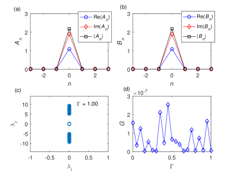
Figure 1: (a),(b) Binary one-site compactons (16) localized at $n=0$, for the case $\sigma=0,\Omega=0$ and with $A_{0}=B_{0}=a+ib$ with $a=0.5\sqrt{\xi_{1}/\alpha}$ and $b=\sqrt{\xi_{1}/\alpha-a^{2}}$. Other parameters are fixed as $\varGamma=1,\gamma_{1}=\gamma_{2}=-1$, $\gamma^{(0)}=-0.5$, $\gamma^{(1)}=0.5$, $\omega=1.0$. (c) The eigenvalue spectrum at $\varGamma=1$, (d) Gain $G$ versus $\varGamma$.

III Stationary conditions for SOC-compactons

We look for stationary SOC-compactons of the form:

$$U_{n}=A_{n}e^{-i\mu_{1}t},\quad V_{n}=B_{n}e^{-i\mu_{2}t},$$ (13)

with $A_{n}$, $B_{n}$ complex amplitudes and $\mu_{1}$, $\mu_{2}$ chemical potentials for the two BEC components. By substituting these expressions into the averaged equations for $U_{n}$, $V_{n}$ given in the Appendix, one finds that all the time dependent exponential factors can be cancelled out except the ones that are proportional to $\Omega$, these being of the form:

$$\Omega e^{-i(\mu_{1}+\mu_{2})t}\Big{\{}\alpha A_{n}^{2}B_{n}^{*}e^{2i\mu_{2}t}J_{1}(\alpha\theta_{0})\;\;\;\;\;\;\;\;\;\;\;\;$$ (14)

$$\;\;\;\;\;\;\;\;-e^{2i\mu_{1}t}B_{n}\Big{[}J_{0}(\alpha\theta_{0})-\alpha|A_{n}|^{2}J_{1}(\alpha\theta_{0})\Big{]}\Big{\}}$$

for Eq. (27), and similar expression for Eq. (28) but with the exchanges $A\leftrightarrow B$ and $\mu_{1}\leftrightarrow\mu_{2}$. From these expressions it is clear that stationary SOC-compactons are possible only if $\Omega=0$ or if the chemical potentials of the two species are equal, i.e. $\mu_{1}=\mu_{2}\equiv\mu$. The corresponding steady-state equations then are:

$$\mu_{1}A_{n}=F_{1}|_{\Omega=0},\,\,\mu_{2}B_{n}=F_{2}|_{\Omega=0},$$ (15)

for case $\Omega=0$, and

$$\mu A_{n}=F_{1},\,\,\,\mu B_{n}=F_{2},$$ (16)

for case $\mu_{1}=\mu_{2}=\mu$. Here $F_{1}$ and $F_{2}$ denote the right hand side of Eqs.(27) and (28), respectively, but with the replacements: $U_{n}\rightarrow A_{n}$, $V_{n}\rightarrow B_{n}$. We remark that although the above stationary conditions are specific of the intra-SOC system, similar conditions would appear also for the inter-SOC system Note2 .

As we shall see in the next section, the condition $\Omega=0$ is too restrictive and can be satisfied only for one-site compactons. In this case, however, although the stability of the solutions will be influenced by the SOC, the analytical expression of the solutions will be the same as for the non-SOC case.

Note that Eq. (16) implies the equality of the number of atoms $N_{1},N_{2}$ in the two components, this being true in general also for multi-site SOC-compactons. This can be easily understood from the fact that for $N_{1}\neq N_{2}$ and $\Omega\neq 0$, there will be oscillations in the number of atoms that will make the zero tunneling conditions at the compacton edges impossible to satisfy. The only way to avoid this is to equilibrate the two components. This, however, requires the additional restriction of the equality of the intra-species interactions (see below).

IV Existence conditions for SOC-compactons

The conditions for the existence of stationary compactons are obtained from Eqs.(15), once the following compacton ansatz is adopted

$$\begin{gathered}A_{n},\,B_{n}\neq 0\;\mbox{\;\;\;\;\; if\;\;$n_{0}-s\leq n\leq n_{0}+s$},\\ A_{n},\,B_{n}=0\;\;\;\;\;\;\mbox{otherwise,\;\;\;\;\;\;\;\;\;\;\;\;\;\;\;\;\;\;\;}\end{gathered}$$ (17)

with $n_{0}-s$ and $n_{0}+s$ denoting the left and right edge of the compacton, respectively, and $s+1$ its width. Since the coupling in the stationary equations involves only first next neighbors, the substitution of the ansatz $\eqref{eq:013}$ into either Eq. (15) or Eq. (16) will give $2(s+3)$ nontrivial equations in correspondence of sites $n_{0}-s-1,...,n_{0},...,n_{0}+s+1,$, with all the others, $n\leq n_{0}-s-2$ and $n\geq n_{0}+s+2$, automatically satisfied. The compacton existence relies on the possibility to solve these $2(s+3)$ equations for the nonzero amplitudes by achieving both the tunneling suppression at the compacton edges and the fixing of the chemical potentials.

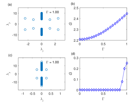
Figure 2: Parameters for panels (a) and (b) are fixed as in panels (c) and (d) of Fig. 1 except $\sigma=1$ and for panels (c) and (d), the parameters are fixed as in (a) and (b) except $\Omega=-2$.

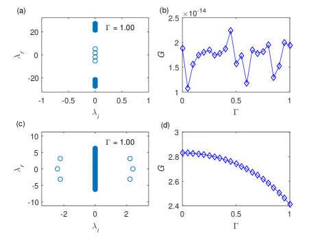
Figure 3: Linear stability analysis for the one-site compactons , (a) The eigenvalue spectrum for case $\varGamma=1,\gamma_{1}=\gamma_{2}=-1$, $\gamma^{(0)}=-1$, $\gamma^{(1)}=0.2$, $\omega=1.0$, $\Omega=-0.4,\sigma=1$, (b) Gain $G$ versus $\varGamma$ with parameters as in (a), (c) The eigenvalue spectrum for case $\varGamma=1,\gamma_{1}=\gamma_{2}=-1$, $\gamma^{(0)}=-0.2$, $\gamma^{(1)}=1$, $\omega=1$ , $\Omega=-0.4,\sigma=1$, (d) Gain $G$ versus $\varGamma$ with parameters as in (c).

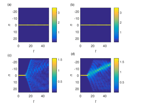
Figure 4: Space-time evolution of the on-site compactons by solving Eq. (7) with $\epsilon=0.01$ , (a) $\left|u_{n}\right|$ and (b) $\left|v_{n}\right|$ for stable case as in Fig.3(a) while (c) $\left|u_{n}\right|$ and (d) $\left|v_{n}\right|$ for unstable case as in Fig. 3(c).

IV.1 One-site SOC-compactons

For a one-site compacton the condition $\Omega=0$ implies existence conditions completely independent on the SOC parameters $\sigma,\Omega$ and therefore will be similar to the case of BEC mixtures in absence of SOC considered in previous papers Abdullaev2 ; Abdullaev3 . On the other hand, for $N_{1}=N_{2}=N/2$ the compacton existence will depend on $\Omega$ but not on $\sigma$, this is because the $\sigma$ term always involves as a factor a zero amplitude on a site $n_{0}\pm 1$ different to the site $n_{0}$. In both cases, however, the SOC terms will strongly influence the stability, therefore it is worth considering in more detail the existence conditions for these two cases.

Case $\Omega=0.$

We take $s=0$ in Eq. (17) and fix the amplitudes at site $n_{0}$ as $A_{n_{0}}=a+ib$, $B_{n_{0}}=c+id$, with $a,b,c,d$ reals and by substituting into Eqs. (15), one obtains in correspondence to sites $n_{0}\pm 1$ four equations that are automatically satisfied if $J_{0}(\alpha(c^{2}+d^{2}))=0$ and $J_{0}(\alpha(a^{2}+b^{2}))=0$, e.g., if $a,b,c,d$ are taken as

$$a^{2}+b^{2}=N_{1}=\frac{\xi_{m}}{\alpha},\;\;c^{2}+d^{2}=N_{2}=\frac{\xi_{l}}{\alpha},$$ (18)

with $\xi_{m},\xi_{l}$ two different zeros of the Bessel function $J_{0}$. One can then check that the other two equations, e.g., the ones for the site $n_{0}$, give the chemical potentials as

$$\mu_{1}=N_{2}\gamma^{(0)}+N_{1}\gamma_{1},\quad\mu_{2}=N_{1}\gamma^{(0)}+N_{2}\gamma_{2}.$$ (19)

Case ${\bf\Omega\neq 0.}$

In this case, we must have $N_{1}=N_{2}=N/2$, so we fix $s=0$ in Eq. (17) and take $A_{n_{0}}=B_{n_{0}}=a+ib$, with $a,b$ reals. One can check that the equations in correspondence to the edges $n_{0}\pm 1$ are automatically satisfied if $J_{0}(\alpha(a^{2}+b^{2}))=0$, e.g., if $a^{2}+b^{2}=N/2=\xi_{l}/\alpha$, with $\xi_{l}$ a zeros of $J_{0}$. The other two equations for the site $n_{0}$ can be solved for the chemical potential only if $\gamma_{1}=\gamma_{2}\equiv\tilde{\gamma}$, this giving:

$$\mu=\frac{N}{2}(\gamma^{(0)}+\tilde{\gamma})+\Omega.$$ (20)

Note that in this case $\Omega$ enters the $\mu$ expressions simply as a shift.

IV.2 Two-site SOC-compactons

For a two-site compacton, $\Omega=0$ will not provide real solutions for the chemical potentials due to the presence of imaginary terms proportional to $\sigma$. It is possible however to eliminate such terms by considering some suitable ansatzes for the amplitudes. For this, let us fix $s=1$ in Eq. (17) and take $A_{n_{0}}=B_{n_{0}+1}=a+ib$, $B_{n_{0}}=A_{n_{0}+1}=a-ib$, with $a,b$ reals (in-phase solution). From Eqs. (16) one then obtains eight equations in correspondence of sites $n_{0}-1,n_{0},n_{0}+1,n_{0}+2$. One can show that these equations lead to the following solution for the chemical potential

$$\mu=\left(a^{2}+b^{2}\right)\left(\frac{\Omega-\varGamma}{a^{2}-b^{2}}+\gamma+\gamma^{(0)}\right),$$ (21)

with $a,b$ given by

$$\begin{gathered}a^{2}=\frac{\xi_{l}}{2\alpha}\left(1+\frac{\Omega-\varGamma}{\sqrt{(\varGamma-\Omega)^{2}+\sigma^{2}}}\right),\\ b^{2}=\frac{\xi_{l}}{2\alpha}\left(1-\frac{\Omega-\varGamma}{\sqrt{(\varGamma-\Omega)^{2}+\sigma^{2}}}\right),\end{gathered}$$ (22)

and $\xi_{l}$ denoting a zero of $J_{0}$. Using Eqs. (22) one can rewrite Eqs. (21) in a more explicit form

$$\mu=\frac{N}{4}\left(\gamma+\gamma^{(0)}\right)+\sqrt{\sigma^{2}+(\varGamma-\Omega)^{2}},$$ (23)

showing the full dependence on parameters $\varGamma,\sigma,\Omega$ and on the total numbers of atoms $N$.

Similarly, one can obtain out-of-phase two-site compactons solutions by assuming the ansatz $A_{n_{0}}=-B_{n_{0}+1}=a+ib$, $B_{n_{0}}=-A_{n_{0}+1}=a-ib$. In this case, the expressions for $\mu,a,b$ are the same as in Eqs. (21) - (23), except for the replacement $\varGamma\rightarrow-\varGamma$ in all equations and for the change of sign in front of the fractions appearing inside the parenthesis in Eqs. (22).

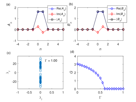
Figure 5: Two-site in-phase compacton for case $\gamma_{1}=\gamma_{2}=1$, $\gamma^{(0)}=4$, $\gamma^{(1)}=1$, $\omega=1$, $\Omega=4$ and $\sigma=1$

.

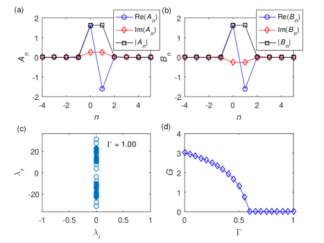
Figure 6: Two-site out-phase compacton for case $\gamma_{1}=\gamma_{2}=-1$, $\gamma^{(0)}=-4$,$\gamma^{(1)}=1$, $\omega=1$, $\Omega=-4$ and $\sigma=1$

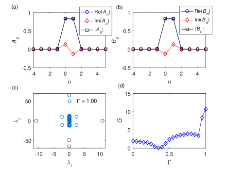
Figure 7: Two-site in-phase compacton for case $\gamma_{1}=\gamma_{2}=1$, $\gamma^{(0)}=4$, $\gamma^{(1)}=8.0$, $\omega=1$, $\Omega=4$ and $\sigma=1$

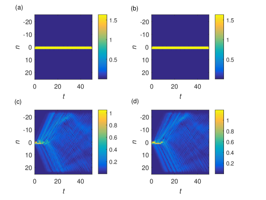
Figure 8: Space-time evolution of the two-site compactons obtained from numerical integrations of Eq. (7) with $\epsilon=0.01$: (a) $\left|u_{n}\right|$ and (b) $\left|v_{n}\right|$ for the stable case at $\Gamma=1$ in Fig.5; (c) $\left|u_{n}\right|$ and (d) $\left|v_{n}\right|$ for unstable case at $\Gamma=1$ in Fig.7.

IV.3 Multi-site SOC-compactons

In principle, the above analysis, being completely general, can be applied to SOC-compactons of arbitrary size. The equations to solve, however, in these cases become much more involved for an exact analysis and one must recourse to numerical methods. An example of this is given for a three-site compacton in the next section.

V Numerical results

In order to check the above results, we will use both linear stability analysis and direct numerical integrations of the original discrete CGPE equations in Eq. (7). For the linear stability analysis, the standard procedure is employed by considering the ansatz with perturbation of the form:

$$\begin{gathered}U_{n}=[A_{n}+\varepsilon(a_{n}e^{-i\lambda t}+b_{n}e^{i\lambda^{*}t})]e^{-i\mu t},\\ V_{n}=[B_{n}+\varepsilon(c_{n}e^{-i\lambda t}+d_{n}e^{i\lambda^{*}t})]e^{-i\mu t},\end{gathered}$$ (24)

where $\lambda=\lambda_{r}+i\lambda_{i}$ denotes the linearization eigenvalue and $\varepsilon\ll{1}$. Substituting Eq. (24) in Eqs. (27), (28) and taking only the terms with $O\left(\varepsilon\right)$ (linear terms of $\varepsilon$), one obtains an eigenvalue problem for $\lambda$ that can be solved numerically. Ideally, the perturbation part in Eq. (24) will remain small (stable) if all imaginary eigenvalues $\lambda_{i}$ are zeros or negligibly small, for gain $G=\max\left(\left|\lambda_{i}\right|\right)\simeq 0$.

Typically, the results of the linear stability analysis of SOC-compactons are further checked by direct integrations of both the averaged and original equations Eq. (7). Since they are found in agreement, however, results in the following will be reported only for the original equations.

V.1 One-site SOC-compactons

As discussed above, the existence condition for one-site SOC-compactons, apart possible shifts of the chemical potential by $\Omega$, are the same as in the absence of SOC. This, however, does not imply that there is no effects of the SOC on compactons because both $\sigma$ and $\Omega$ can strongly influence their stability.

We show this by comparing results of the linear stability analysis in the case of absence of SOC , i.e. $\sigma=0,\Omega=0$, (see Fig. 1) with the ones obtained in the presence of SOC (see Figs.2 and 3). From Fig. 1 we see that the linear spectrum has a gain $G$ that is practically zero for all $\varGamma\in\left[0,1\right]$, meaning that the solutions are stable, a fact that is already known from previous results Abdullaev3 . By increasing $\sigma$ away from zero but retaining $\Omega=0$, we find that the solution becomes unstable (see panels a, b of Fig. 2) for the case $\sigma=1,\Omega=0$. This instability, however, is physically not very significative because the SOC implementation usually requires both $\sigma,\Omega$ to be nonzero. By increasing also $|\Omega|$ away from zero, the stability can be restored almost for the whole range in $\varGamma$ of the zero SOC case, as one can see from panels (c, d) of Fig. 2, for the case $\sigma=1,\Omega=-2$. Similar results are obtained for different choices of the system parameters and for different compacton amplitudes. In general, we have that stable one-site SOC-compactons can exist in wide regions of the parameter space.

We have also investigated the effects of the nonlinearity management parameters $\gamma^{(0)}$, $\gamma^{(1)}$, on the stability of one-site SOC-compactons. Note from Eq. (18) that the compacton amplitude is inversely proportional to the value of $\gamma^{(1)}$, despite $\gamma^{(1)}$ alone does not affect the stability. Remarkably, the solutions become significantly stable when $\left|\gamma^{(0)}\right|$ is much larger than $\gamma^{(1)}$ as demonstrated in Fig. 3(a, b) and, oppositely, the solutions become unstable when $\left|\gamma^{(0)}\right|$ is much lower than $\gamma^{(1)}$, as portrayed in Fig. 3 (c, d). The above linear stability results are further confirmed by nonlinear stability analysis achieved via numerical time-integrations of the nonlinear system in Eq. (7), as one can see from Fig. 4.

V.2 Two-site SOC-compactons

For multi-site compactons, we must necessarily to have the condition $\Omega\neq 0$, i.e. equal chemical potentials for the two BEC components and this implies equal intra-species interactions. Let us consider first the case of an in-phase SOC-compacton with amplitudes $A_{0}=B_{1}=a+ib,A_{1}=B_{0}=a-ib,$ with $a=\sqrt{\xi_{1}/2\alpha}$, $b=\sqrt{\xi_{1}/\alpha-a^{2}}$. We fix parameters as: $\gamma_{1}=\gamma_{2}=1$, $\gamma^{(0)}=4$, $\gamma^{(1)}=1$, $\omega=1$, $\Omega=4$, $\sigma=1$. Note that all the nonlinear parameters here are positive, i.e interactions are repulsive. In panels a,b of Fig. 5 we show the real and imaginary parts versus $n$ of the first and second component $A_{n},B_{n}$ , respectively, of a two-site in-phase compactons, while in the bottom panels (c,d) their stability analysis is reported as a function of the parameter $\Gamma$. From panel d) it is clear that for $\Gamma$ less than $\approx 0.6$ the gain $G$ is positive and the solution is unstable, while for all $\Gamma\geq 0.6$ the gain reduces to zero and the solution becomes stable. The panel c of the figure just shows the stability in terms of the linear eigenvalues at $\Gamma=1$ from which we see that they are all real numbers.

Similarly, for an out-of-phase two-site compacton we fix the amplitudes as: $A_{0}=-B_{1}=a+ib$, $B_{0}=-A_{1}=a-ib$, with the same $a$, $b$ of the previous case. Parameters are fixed as $\gamma_{1}=\gamma_{2}=-1$, $\gamma^{(0)}=-4$, $\gamma^{(1)}=1$, $\omega=1$, $\Omega=-4$, $\sigma=1$. Results, are reported in Fig. 6, where panels (a, b) depict the solutions of typical out-of-phase profiles and panels (c,d) show the results from the stability analysis. Notice that despite the type of interactions is changed from repulsive to attractive, the range of stability is the same as for the in-phase case. Thus, independently on the sign of the interaction, in the interval $0.6\leq\varGamma\leq 1$ both the in-phase and the out-of phase compactons appear to be stable. This is quite interesting because it shows SOC-compacton bistability in contrast with usual inter-site breathers (i.e. localized out-of-phase solutions with tails) which are known to be unstable in conventional (i.e. in absence of SNM) SOC-BEC mixtures Belicev .

The stability of the solution also depends on the ratio $\eta=\gamma^{(0)}<\gamma^{(1)}$ between the dc and ac strengths of the inter-site interaction, with the two-site SOC-compacton becoming unstable for $\eta<1$. This is shown in Fig.7 for the case of the same two-site in-phase compacton depicted in Fig. 5 but with $\eta=0.5$.

Finally, we find the results of the linear stability analysis to be in very good agreement with those obtained from direct numerical integrations of Eq. (7). An example of this is shown in Fig.8 where the stable and unstable time evolution of the two-site in-phase compactons of Fig.s 5 and 7 at $\Gamma=1$, are reported.

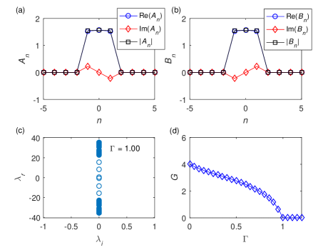
Figure 9: Three-site compacton for case $\gamma_{1}=\gamma_{2}=1$, $\gamma^{(0)}=10$, $\gamma^{(1)}=1$, $\omega=1$, $\Omega=4$ and $\sigma=1$.

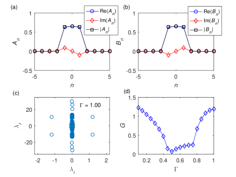
Figure 10: Three-site compacton for case $\gamma_{1}=\gamma_{2}=1$, $\gamma^{(0)}=10$, $\gamma^{(1)}=6.0$, $\omega=1$, $\Omega=4$ and $\sigma=1$.

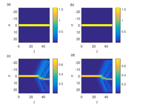
Figure 11: Space-time evolution of the three-site compactons obtained from numerical integrations of Eq. (7) with $\epsilon=0.01$, (a) $\left|u_{n}\right|$ and (b) $\left|v_{n}\right|$ for the stable case at $\Gamma=1$ in Fig.9; (c) $\left|u_{n}\right|$ and (d) $\left|v_{n}\right|$ for unstable case at $\Gamma=1$ in Fig.10.

V.3 Three-site SOC-compactons

Three-site SOC-compacton solutions are obtained from Eq. (17) with $s=2$ by taking $\mu_{1}=\mu_{2}=\mu$ and assuming the following ansatz for the solution: $A_{n_{0}}=a+ib$, $B_{n_{0}}=a-ib$, $A_{n_{0}\pm 1}=c+id$ and $B_{n_{0}\pm 1}=c-id$, with $a,b,c,d$ real numbers. Direct substitution of the ansatz into Eq. (16) provides ten equations which are reduced to six (for instance only those for sites $n_{0}-2,n_{0}-1,n_{0}$) thanks to the symmetry of the solution around the central site $n_{0}$. From the equations for the site $n_{0}-2$ one obtains the zero tunneling conditions for $A_{n_{0}\pm 2},B_{n_{0}\pm 2}$ at the edges of the compacton in terms of roots of the Bessel function as in Eq. (18). Substituting these conditions into the equation relative to sites $n_{0}-1$ one obtains two equations that can be combined into the following expression for the chemical potential:

$$\mu = -\frac{1}{Re\left(w_{2}\right)}\left[\alpha\varGamma\left(Re\left(w_{2}\bar{z}_{1}w_{1}\right)\right.\right.$$

$$\left.+Re\left(w_{2}z_{1}\bar{w}_{1}\right)\right)J_{1}\left(\alpha\left(\left|z_{2}\right|^{2}-\left|w_{2}\right|^{2}\right)\right)$$

$$+\varGamma Re\left(z_{2}\right)J_{0}\left(\alpha\left(\left|z_{1}\right|^{2}-\left|w_{1}\right|^{2}\right)\right)$$

$$-\Omega Re\left(w_{1}\right)-\gamma\left|w_{1}\right|^{2}Re\left(w_{2}\right)$$

$$-\gamma^{\left(0\right)}\left|w_{1}\right|^{2}Re\left(w_{2}\right)$$

$$-\alpha\sigma J_{1}\left(\alpha\left(\left|z_{2}\right|^{2}-\left|w_{2}\right|^{2}\right)\right)\cdot$$

$$\left(Im\left(w_{2}\bar{z}_{1}w_{1}\right)-Im\left(w_{2}z_{1}\bar{w}_{1}\right)\right)$$

$$-\sigma J_{0}\left(\alpha\left(\left|z_{1}\right|^{2}-\left|w_{1}\right|^{2}\right)\right)\left.Im\left(z_{2}\right)\right].$$

Here we used $\gamma_{1}=\gamma_{2}=\gamma$ and denoted $z_{1}=a+ib,z_{2}=a-ib,w_{1}=c+id,w_{2}=c-id$. Lastly, from the equations for site $n_{0}$ one gets:

$$\mu z_{j+1}+2\alpha\varGamma z_{j+1}\left(\bar{w}_{2-j}z_{2-j}+w_{2-j}\bar{z}_{2-j}\right)\cdot$$

$$J_{1}\left(\alpha\left(\left|w_{j+1}\right|^{2}-\left|z_{j+1}\right|^{2}\right)\right)$$

$$+\alpha\varOmega\left(z_{2-j}\left|z_{j+1}\right|^{2}+z_{2-j}z_{j+1}^{2}\right)\cdot$$

$$J_{1}\left(\alpha\left(\left|z_{j+1}\right|^{2}-\left|z_{2-j}\right|^{2}\right)\right)$$

$$+2\varGamma w_{j+1}J_{0}\left(\alpha\left(\left|w_{2-j}\right|^{2}-\left|z_{2-j}\right|^{2}\right)\right)$$

$$-\varOmega z_{2-j}J_{0}\left(\alpha\left(\left|z_{j+1}\right|^{2}-\left|z_{2-j}\right|^{2}\right)\right)$$

$$-\gamma\left|z_{j+1}\right|^{2}z_{j+1}-\gamma^{\left(0\right)}\left|z_{2-j}\right|^{2}z_{j+1} = 0,$$

with $j=0,1$. These nonlinear equations together with the previous ones should be solved numerically for $a,b,c,d$ giving the the compacton amplitudes of the two components at sites $n_{0},n_{0}\pm 1$.

Stability patterns for three-site compactons are in general similar to the ones previously investigated but for $\sigma=1$ or larger it is more difficult to obtain stable solutions unless $\varGamma\geq 1$, as shown in Fig. 9. Another distinctive feature in this case is the absence of stable solutions $\gamma^{(0)}<\gamma^{(1)}$, and even for $\gamma^{(0)}>\gamma^{(1)}$, if the difference is not sufficiently large, the solution might become unstable as depicted in Fig. 10. Lastly, in the top and bottom panels of Fig. 11 we report the time evolution obtained from numerical integrations of Eq. (7) by initial conditions the solutions at $\Gamma=1$ depicted in Fig. 9 and Fig. 10, for which the linear stability analysis predicts stability and instability, respectively. As one can see from panels (a,b) and (c,d) of Fig. 11 these predictions are fully confirmed.

VI Conclusions

In this paper we have investigated the existence and stability properties of compactons matter waves excitations of binary BEC mixtures with spin-orbit coupling trapped in an OL, subjected to SNM. We considered for simplicity an inter-SOC system (i.e. with an off-diagonal Rabi term) and assumed both the OL to be deep enough to justify the tight-binding approximation and the strength and the frequency of the modulation to be large enough to use the averaging method.

Within this model, we derived effective averaged equations of motion for the matter wave complex amplitudes in the form of a two coupled discrete NLS and demonstrated that the SNM introduces a local density imbalance dependence not only in the tunneling parameter $\Gamma$ but also in the SOC parameters $\sigma$ and $\Omega$. This density dependence of the SOC parameters persists in the system independently on the SOC-compacton existence.

The dependence of both $\sigma$ and $\Omega$ on the local density imbalance, however, give rise to conditions for stable SOC-compactons existence that are more restrictive than the ones obtained in the absence of SOC. In general, the stationarity condition requires the equality of the chemical potentials of the two components, a fact that can be satisfied when the number of atoms of the two species are equal as well as their intra-species nonlinearities. We have also investigated the stability of SOC-compactons versus the system parameters, i.e. the SOC strength $\sigma$, the Rabi frequency $\Omega$, the coupling or hopping constant $\varGamma$ and the ratio between the nonlinear coefficients $\gamma^{(0)},\gamma^{(1)}$. This has been done both using a linear stability analysis of the averaged equations and by direct numerical time integrations of the original nonlinear PDE equations. Numerical simulations show that by keeping the other parameters fixed, an enlargement of the stability region of SOC-compactons can be achieved by decreasing $\sigma$ or by increasing $\Omega$. Stability seems also more easily obtainable for $\left|\gamma^{(0)}\right|>\left|\gamma^{(1)}\right|$ and large values of $\varGamma$.

From this, we conclude that while on one side the SOC restricts the parameter range for stationary SOC-compacton existence, on the other side it gives a more stringent signature of their occurrence. Indeed, they should appear when the intra-species interactions and the number of atoms in the two components are perfectly balanced (or close to being balanced for metastable cases). This suggests SOC-compactons as possible tools for indirect measurements of the number of atoms, and/or the intra-species interactions, in experiments.

VII APPENDIX: Averaged equations and Hamiltonian structure

Below we provide the derivation of the averaged system Eq. (13). By substituting Eq. (10) into Eq. (7) we get:

$$iU_{n,t}= -i\varGamma U_{n}(\langle\Lambda\bar{X}_{1}^{+}\rangle V_{n}-\langle\Lambda X_{1}^{+}\rangle V_{n}^{*})$$

$$-\sigma U_{n}(\langle\Lambda\bar{X}_{1}^{-}\rangle V_{n}+\langle\Lambda X_{1}^{-}\rangle V_{n}^{*})$$

$$+i\Omega(\langle\Lambda\bar{X}_{0}^{+}\rangle V_{n}|U_{n}|^{2}-\langle\Lambda X_{0}^{-}\rangle V_{n}^{*}U_{n}^{2})$$

$$-\varGamma\langle X_{2}^{+}\rangle+i\sigma\langle X_{2}^{-}\rangle+\Omega\langle X_{0}^{-}\rangle V_{n}$$

$$+\gamma_{1}|U_{n}|^{2}U_{n}+\gamma^{(0)}|V_{n}|^{2}U_{n},$$ (25)

$$iV_{n,t}= -i\varGamma V_{n}(\langle\Lambda\bar{X}_{2}^{+}\rangle U_{n}-\langle\Lambda X_{2}^{+}\rangle U_{n}^{*})$$

$$+\sigma V_{n}(\langle\Lambda\bar{X}_{2}^{-}\rangle U_{n}+\langle\Lambda X_{2}^{-}\rangle U_{n}^{*})$$

$$+i\Omega(\langle\Lambda\bar{X}_{0}^{+}\rangle U_{n}|V_{n}|^{2}-\langle\Lambda X_{0}^{-}\rangle U_{n}^{*}V_{n}^{2})$$

$$-\varGamma\langle X_{1}^{+}\rangle-i\sigma\langle X_{1}^{-}\rangle+\Omega\langle X_{0}^{+}\rangle U_{n}$$

$$+\gamma_{2}|V_{n}|^{2}V_{n}+\gamma^{(0)}|U_{n}|^{2}V_{n}.$$ (26)

where

$$X_{2}^{\pm} =U_{n+1}e^{i\Lambda(|{V_{n+1}}|^{2}-|{V_{n}}|^{2})}\pm U_{n-1}e^{i\Lambda(|{V_{n-1}}|^{2}-|{V_{n}}|^{2})},$$

$$X_{1}^{\pm} =V_{n+1}e^{i\Lambda(|{U_{n+1}}|^{2}-|{U_{n}}|^{2})}\pm V_{n-1}e^{i\Lambda(|{U_{n-1}}|^{2}-|{U_{n}}|^{2})},$$

$$X_{0}^{\pm} =e^{\pm i\Lambda(|{U_{n}}|^{2}-|{V_{n}}|^{2})}.$$

and $\langle\cdot\rangle$ is the rapid modulated term to be averaged. The averaged terms can be evaluated as:

$$\langle\Lambda X_{1}^{\pm}\rangle=V_{n+1}\langle\Lambda e^{i\Lambda\theta_{1}^{+}}\rangle\pm V_{n-1}\langle\Lambda e^{i\Lambda\theta_{1}^{-}}\rangle,$$

$$\langle\Lambda X_{2}^{\pm}\rangle=U_{n+1}\langle\Lambda e^{i\Lambda\theta_{2}^{+}}\rangle\pm U_{n-1}\langle\Lambda e^{i\Lambda\theta_{2}^{-}}\rangle,$$

$$\langle X_{1}^{\pm}\rangle=V_{n+1}\langle e^{i\Lambda\theta_{1}^{+}}\rangle\pm V_{n-1}\langle e^{i\Lambda\theta_{1}^{-}}\rangle,$$

$$\langle X_{2}^{\pm}\rangle=U_{n+1}\langle e^{i\Lambda\theta_{2}^{+}}\rangle\pm U_{n-1}\langle e^{i\Lambda\theta_{2}^{-}}\rangle,$$

$$\langle\Lambda X_{0}^{\pm}\rangle=\langle\Lambda e^{\pm{i}\Lambda\theta_{0}}\rangle,\quad\langle X_{0}^{\pm}\rangle=\langle e^{\pm{i}\Lambda\theta_{0}}\rangle,$$

with $\theta_{1}^{\pm}=|U_{n\pm 1}|^{2}-|U_{n}|^{2}$, $\theta_{2}^{\pm}=|V_{n\pm 1}|^{2}-|V_{n}|^{2}$ and $\theta_{0}=|U_{n}|^{2}-|V_{n}|^{2}$ and furthermore

$$\langle\Lambda e^{\pm{i}\Lambda\theta_{j}^{\pm}}\rangle =\frac{\omega}{2\pi}\int_{0}^{2\pi/\omega}\frac{\gamma^{(1)}}{\omega}\sin(\omega\tau)e^{\pm{i}\frac{\gamma^{(1)}}{\omega}\theta_{j}^{\pm}\sin(\omega\tau)}\ d\tau$$

$$=\pm{i}\alpha J_{1}(\alpha\theta_{j}^{\pm}),\;\;\;\;\;\langle e^{\pm{i}\Lambda\theta_{j}^{\pm}}\rangle=J_{0}(\alpha\theta_{j}^{\pm}),$$

$$\langle\Lambda e^{\pm{i}\Lambda\theta_{0}}\rangle =\pm i\alpha{J_{1}}(\alpha\theta_{0}),\;\;\;\;\;\langle e^{\pm{i}\Lambda\theta_{0}}\rangle=J_{1}(\alpha\theta_{0}),$$

where $\alpha=\gamma^{(1)}/\omega$ and $J_{0}$, $J_{1}$ are the Bessel functions of order 0 and 1 respectively. Substituting the averages into Eqs.(25) and (26) yields:

$$i U_{n,t}=-\varGamma\Big{\{}\alpha U_{n}\Big{[}(V_{n+1}^{*}V_{n}+V_{n+1}V_{n}^{*})J_{1}(\alpha\theta_{1}^{+})+$$

$$(V_{n-1}^{*}V_{n}+V_{n-1}V_{n}^{*})J_{1}(\alpha\theta_{1}^{-})\Big{]}+U_{n+1}J_{0}(\alpha\theta_{2}^{+})+$$

$$U_{n-1}J_{0}(\alpha\theta_{2}^{-})\Big{\}}+\Big{\{}\gamma_{1}|U_{n}|^{2}+\gamma^{(0)}|V_{n}|^{2}\Big{\}}U_{n}+$$ (27)

$$i\sigma\Big{\{}\alpha U_{n}\Big{[}(V_{n+1}^{*}V_{n}-V_{n+1}V_{n}^{*})J_{1}(\alpha\theta_{1}^{+})-(V_{n-1}^{*}V_{n}-$$

$$V_{n-1}V_{n}^{*})J_{1}(\alpha\theta_{1}^{-})\Big{]}+U_{n+1}J_{0}(\alpha\theta_{2}^{+})-U_{n-1}J_{0}(\alpha\theta_{2}^{-})\Big{\}}$$

$$-\Omega\Big{\{}\alpha J_{1}(\alpha\theta_{0})(V_{n}|U_{n}|^{2}+V_{n}^{*}U_{n}^{2})-V_{n}J_{0}(\alpha\theta_{0})\Big{\}},$$

$$i V_{n,t}=-\varGamma\Big{\{}\alpha V_{n}\Big{[}(U_{n+1}^{*}U_{n}+U_{n+1}U_{n}^{*})J_{1}(\alpha\theta_{2}^{+})+$$

$$(U_{n-1}^{*}U_{n}+U_{n-1}U_{n}^{*})J_{1}(\alpha\theta_{2}^{-})\Big{]}+V_{n+1}J_{0}(\alpha\theta_{1}^{+})+$$

$$V_{n-1}J_{0}(\alpha\theta_{1}^{-})\Big{\}}+\Big{\{}\gamma_{2}|V_{n}|^{2}+\gamma^{(0)}|U_{n}|^{2}\Big{\}}V_{n}-$$ (28)

$$i\sigma\Big{\{}\alpha V_{n}\Big{[}(U_{n+1}^{*}U_{n}-U_{n+1}U_{n}^{*})J_{1}(\alpha\theta_{2}^{+})-(U_{n-1}^{*}U_{n}-$$

$$U_{n-1}U_{n}^{*})J_{1}(\alpha\theta_{2}^{-})\Big{]}+V_{n+1}J_{0}(\alpha\theta_{1}^{+})-V_{n-1}J_{0}(\alpha\theta_{1}^{-})\Big{\}}$$

$$+\Omega\Big{\{}\alpha J_{1}(\alpha\theta_{0})(U_{n}|V_{n}|^{2}+U_{n}^{*}V_{n}^{2})+U_{n}J_{0}(\alpha\theta_{0})\Big{\}}.$$

Furthermore, the pdes Eqs. (27) and (28) can be written in terms of $iU_{n,t}=\delta H_{av}/\delta U_{n}^{*}$ and $iV_{n,t}=\delta H_{av}/\delta V_{n}^{*}$ respectively, where the averaged Hamiltonian is:

$$H_{av}= \sum_{n}\Big{[}-\varGamma J_{0}(\alpha\theta_{2}^{+})(U_{n+1}U_{n}^{*}+U_{n+1}^{*}U_{n})$$ (29)

$$-\varGamma J_{0}(\alpha\theta_{1}^{+})(V_{n+1}V_{n}^{*}+V_{n+1}^{*}V_{n})$$

$$+i\sigma J_{0}(\alpha\theta_{2}^{+})(U_{n+1}U_{n}^{*}-U_{n+1}^{*}U_{n})$$

$$-i\sigma J_{0}(\alpha\theta_{1}^{+})(V_{n+1}V_{n}^{*}-V_{n+1}^{*}V_{n})$$

$$+\Omega J_{0}(\alpha\theta_{0})(U_{n}V_{n}^{*}+U_{n}^{*}V_{n})$$

$$+\frac{1}{2}(\gamma_{1}|U_{n}|^{4}+\gamma_{2}|V_{n}|^{2})+\gamma^{(0)}|U_{n}|^{2}|V_{n}|^{2}\Big{]}.$$

By comparing the averaged Hamiltonian in Eq. (29) with the original Hamiltonian Eq. (8), their terms coincide if one rescales the tunneling or hopping constant $\varGamma$, the SOC parameter $\sigma$ and the Rabi frequency $\Omega$ according to Eq. (12). It should be noted here that the averaged equations only valid for $t\leq 1/\epsilon$ with accuracy of $\mathfrak{\mathcal{O}}\left(\epsilon\right)$ Sanders .

References

• (1) M. Bukov, L. D’Alessio, A. Polkovnikov, Advances in Physics, 64, 139226 (2015).
• (2) Y.J. Lin, K. Jiménez-García and I. B. Spielman, Nature, 471, 83–86, (2010).
• (3) V. Galitski and I. B. Spielman, Nature 494, 49–54 (2013).
• (4) F. Kh. Abdullaev, P. G. Kevrekidis, and M. Salerno, Phys. Rev.Lett. 105, 113901 (2010).
• (5) S. Greschner, G. Sun, D. Poletti, and L. Santos, Phys. Rev. Lett. 113, 215303 (2014).
• (6) A. Rapp, X. Deng, and L. Santos, Phys. Rev. Lett. 109, 203005 (2012).
• (7) J. Gong, L. Morales-Molina, and P. Hänggi, Phys. Rev. Lett. 103, 133002 (2009).
• (8) F Meinert, MJ Mark, K Lauber, AJ Daley, HC Nägerl, Phys. Rev. Lett. 116, 205301 (2020).
• (9) F. Kh. Abdullaev, M. S. A. Hadi, M. Salerno, and B. Umarov, Phys. Rev. A 90, 063637 (2014).
• (10) F. Kh. Abdullaev, M. S. A. Hadi, M. Salerno, and B. Umarov, J. Phys. B 50, 16 (2017).
• (11) J. D’Ambroise, M. Salerno, P. G. Kevrekidis, and F. Kh. Abdullaev, Phys. Rev. A 92, 053621 (2015).
• (12) P.P. Belicev, G. Gligoric, J. Petrovic, A. Maluckov, L. Hadievski, B.A. Malomed, J. Phys. B 48, 065301 (2015).
• (13) M. Salerno and F. Kh. Abdullaev, Phys. Lett. A 379, 2252 (2015).
• (14) M. Salerno, F. Kh. Abdullaev, A. Gammal, and Lauro Tomio, Phys. Rev. A 94, 043602 (2016).
• (15) P. Xu, T. Deng, W. Zheng, H. Zhai, Phys Rev. A 103, L061302 (2021).
• (16) G.L. Alfimov, P.G. Kevrekidis, V.V. Konotop, M. Salerno, Phys. Rev. E 66 (2002) 046608.
• (17) S. Sakaguchi, and B. A. Malomed, Symmetry, 11, 388 (2019).
• (18) J.A. Sanders, F. Verhulst, and J. Murdock, Averaging Methods in Nonlinear Dynamical Systems (Springer Science+Business Media, LLC, 2007).
• (19) In the inter-SOC case $\Omega$ is a diagonal Zeeman term while $\sigma$ term is off-diagonal. In this case the terms proportional to $\sigma$ in the averaged equations, will have time dependent factors similar to the ones in (III) but with the roles of $\sigma$ and $\Omega$ interchanged.