1 Introduction

Extremal black holes are objects of great interest to the string theorists, though they concern a pretty ideal situation, as they lack temperature $T$. In the recent past, near-extremal black holes have also been objects of intense study. A near-extremal black hole is a black hole which is not far from saturating the extremality bound, namely which is not far from having the minimal possible mass that can be compatible with the charges, and possible angular momentum (or momenta), of the black hole itself. In supersymmetric theories, near-extremal black holes are often small perturbations of supersymmetric (BPS) black holes; as such, near-extremal black holes have small Hawking temperatures and consequently emit small amounts of Hawking radiation.

Jackiw-Teitelboim (JT) gravity, introduced in the 80’s [1, 2], has recently been exploited in order to study higher-dimensional near-extremal black holes within the two-dimensional dilaton gravity theory obtained upon dimensional reduction [3, 4]. In this framework, it has been shown that as an $AdS_{2}$ factor emerges within the near-horizon geometry of a near-extremal black hole, its dynamics can be effectively described by a two-dimensional dilaton gravity, obtained by dimensional reduction. This results in to a dramatic simplification, opening up new directions within the study of near-extremal black holes. For instance, in recent years, a broad variety of near-extremal black holes has been studied through JT gravity in great detail, ranging from charged to rotational black holes [5, 6], for non-relativistic theories [7] as well as for higher-derivative gravity [8].

A natural question arising in this context is whether the properties of extremal black holes still persist, and, if and how they get changed or deformed when one (slightly) departs from extremality by considering near-extremal black holes. In this paper, we will focus on the Freudenthal duality [9, 10], by investigating whether one can make sense at all of such a property of extremal black holes in Maxwell-Einstein (super)gravity theories in four-space time dimensions when considering near-extremal black holes. Freudenthal duality is an intrinsically non-linear symmetry of the Bekenstein-Hawking entropy of extremal black holes, which, in the case of asymptotically flat and static solutions is also an anti-involutive map in the space of electric and magnetic charges of the black holes themselves [9, 10, 11] (cf. discussion in Sec. 2.3). Within its anti-involutive formulation, Freudenthal duality has been extended to act also on the fluxes supporting flux compactification of string theory, giving rise to gauged supergravity theories in four dimensions [12]; further investigations have been made e.g. in [13]-[18]. Under Freudenthal duality, dyonic charges and fluxes (i.e., gauging parameters) undergo non-linear transformations, which therefore cannot be regarded as electric-magnetic duality (U-duality) transformations, because the latter is linearly realized in the framework under consideration [19, 20, 21]. Remarkably, in extremal black holes also the attractor points, describing the attractor configurations of scalar fields at the (unique) event horizon of the black hole, are invariant under Freudenthal duality [10].

In [22], an attempt has first been made in order to establish how Freudenthal duality acts on near-extremal black holes: the outcome of such an investigation resulted in the statement that two near-extremal black holes cannot be Freudenthal dual (i.e., cannot have the same entropy and temperature, with electric-magnetic (e.m.) charges related by a Freudenthal duality transformation) if their e.m. charges are not related via the Freudenthal duality transformation defined by the corresponding extremal entropy (i.e., by the entropy pertaining to the uniquely defined extremal limit $\lim_{T\rightarrow 0^{+}}$ of the $T$-dependent near-extremal entropy); actually, this breakdown is expected, as the near-extremal entropy is no more a homogeneous function of degree two of the charges [20, 21].

In the present paper, we will show how to circumvent such an obstruction, and thus how to consistently formulate a Freudenthal duality for the entropy of near-extremal black holes; we anticipate that the price to pay for it is a (remarkably, non-linear and uniquely defined) transformation of the temperature $T$ itself.

The plan of the paper is as follows.

In Sec. 2 we review some topics of the framework in which we will derive our results, such as $\mathcal{N}=2$, $D=4$ ungauged supergravity (or, more in general, Maxwell-Einstein theories coupled to a non-linear sigma model of scalar fields in absence of a potential) in Sec. 2.1 and the approach to the entropy of near-extremal black holes based on Jackiw-Teitelboim gravity in Sec. 2.2. We will also comment on the invariance of extremal entropy under Freudenthal duality and on the non-invariance of near-extremal entropy under a naïve notion of Freudenthal duality in presence of a non-vanishing temperature, respectively in Secs. 2.3 and 2.4. Then, in Sec. 3 we present near-extremal Freudenthal duality, which is the consistent generalization of the intrinsically non-linear Freudenthal duality map (originally introduced for extremal black holes) to the class of near-extremal black hole solutions of Einstein-Maxwell equations of motion. In particular, the introduction of a non-linear transformation of the temperature is discussed in Sec. 3.1, whereas its uniqueness and identification with a specific solution of a quartic algebraic equation are discussed in Secs. 3.2 and 3.3, respectively. In Sec. 4 we briefly present an application of our results to the STU model. Concluding remarks and hints for further developments are given in the final Sec. 5. Two appendices conclude the paper, dedicated to the statement of the technical results which we will exploit in order to derive our results: namely, Descartes’ rule of signs (in App. A) and Sturm’s Theorem (in App. B).

2 Freudenthal duality in $\mathcal{N}=2$, $D=4$ ungauged supergravity

2.1 A few basics

Here we will briefly review the observation made by two of the present authors in [22], which dealt with the Freudenthal duality of a near-extremal black hole in type $IIA$, $\mathcal{N}=2$, $D=4$ ungauged supergravity, by exploiting the JT gravity theory. The bosonic part of the corresponding ungauged supergravity action coupled with an arbitrary number of vector multiplets can be written as

$$\mathcal{S} = -\frac{1}{8\pi G_{4}}\int d^{4}x\sqrt{-G}\Bigg{(}-{\frac{R}{2}}+h_{a\bar{b}}\partial_{\mu}x^{a}\partial_{\nu}\bar{x}^{\bar{b}}G^{\mu\nu}$$ (2.1)

$$-\mu_{\Lambda\Sigma}\mathcal{F}_{\mu\nu}^{\Lambda}\mathcal{F}_{\lambda\rho}^{\Sigma}G^{\mu\lambda}G^{\nu\rho}-\nu_{\Lambda\Sigma}\mathcal{F}_{\mu\nu}^{\Lambda}\ast\mathcal{F}_{\lambda\rho}^{\Sigma}G^{\mu\lambda}G^{\nu\rho}\Bigg{)},$$

with $G_{4}$ standing for the four-dimensional Newton’s constant, and $G_{\mu\nu}$, $R$ and $G$ respectively denoting the space-time metric, the Ricci scalar and the determinant of the metric. On the other hand, $h_{a\bar{b}}$ denotes the moduli space metric for the $n$ complex scalars $x^{a}$. The action (2.1) also includes $n+1$ 1-form Maxwell potentials $A_{\mu}^{\Lambda}$, $\Lambda=0,1,...,n$, whose corresponding 2-form field strengths are denoted as $\mathcal{F}^{\Lambda}$.

The action (2.1) can be conceived as the purely bosonic sector of a Maxwell-Einstein supergravity theory arising as the large-volume, low-energy limit of type $IIA$ string theory compactified on some Calabi-Yau threefold $\mathcal{M}$. For this theory, the prepotential $F$ and the Kähler potential $K$ read as

$$F=D_{abc}{\frac{X^{a}X^{b}X^{c}}{X^{0}}},\quad K=-\log\left[i\sum_{\Lambda=0}^{n}\left(\overline{X^{\Lambda}}\partial_{\Lambda}F-X^{\Lambda}\overline{\partial_{\Lambda}F}\right)\right],$$ (2.2)

where $X^{a}=x^{a}X^{0}$. The Kähler potential $K$ yields the moduli space metric $h_{a\bar{b}}=\partial_{a}\partial_{\bar{b}}K$, where the partial derivatives are taken with respect to the complex moduli fields. The gauge coupling constants in (2.1) can be considered to be given by the real and imaginary part of a complex symmetric matrix $\mathcal{N}_{\Lambda\Sigma}$ as $\mu=\text{Im}\mathcal{N}$ and $\nu=-\text{Re}\mathcal{N}$ with

$$\mathcal{N}_{\Lambda\Sigma}=\overline{F_{\Lambda\Sigma}}+2i{\frac{\text{Im}F_{\Lambda\Omega}\text{Im}F_{\Sigma\Pi}X^{\Omega}X^{\Pi}}{\text{Im}F_{\Omega\Pi}X^{\Omega}X^{\Pi}}};\quad F_{\Lambda\Sigma}:=\partial_{\Lambda}\partial_{\Sigma}\,F.$$ (2.3)

Defining the 2-forms $\alpha_{a}$ to be the basis of the second integral cohomology group $H^{2}(\mathcal{M},\mathbb{Z})$, the triple intersection numbers $D_{abc}$ of $\mathcal{M}$ are defined as

$$D_{abc}:=\frac{1}{6}\int_{\mathcal{M}}\alpha_{a}\wedge\alpha_{b}\wedge\alpha_{c}.$$ (2.4)

Nota Bene : while we refer to type $IIA$, $\mathcal{N}=2$, $D=4$ ungauged supergravity for a concrete framework, all results obtained in this paper actually hold irrespective of (local) supersymmetry, namely they actually, hold for any Maxwell-Einstein theory in $D=4$ space-time dimensions with an action given by (2.1). This is a remarkable fact, which was proved within the general treatment firstly given in [10], and then developed and detailed in subsequent works, such as [11], [19], [20] and [21].

2.2 Jackiw-Teitelboim gravity and near-extremal entropy

Before discussing the application of Freudenthal duality to near-extremal black hole, here we will briefly summarize the procedure to derive the near-extremal black hole entropy; further details and comments can be found in [23, 22]. A crucial property is the fact that the near-horizon geometry of an asymptotically flat, static, spherically symmetric, dyonic extremal black hole factorises as $AdS_{2}\otimes S^{2}$, with both factors having the same radius; this results in the so-called Bertotti-Robinson geometry [24, 25]. We will consider the simple case, in which the near-extremal black hole inherits the spherical symmetry and the staticity from its extremal counterpart/limit. In this scenario, one can split the computation of the near-extremal black hole entropy into four steps, briefly listed below [23, 22].

1. Dimensional reduction: The first step is to start with a dimensional reduction, by considering a spherically symmetric Ansatz for the four-dimensional, asymptotically flat black hole metric $G_{\mu\nu}$ as

   $$ds^{2}=G_{\mu\nu}dx^{\mu}dx^{\nu}=\tilde{g}_{\alpha\beta}dx^{\alpha}dx^{\beta}+{\Phi}^{2}d\Omega_{2}^{2};\quad\mu,\nu\in[0,3],\quad\alpha,\beta\in[0,1].$$ (2.5)

   Furthermore, we denote the electric and magnetic charges of the black hole by $Q_{\Lambda}$ and $P^{\Lambda}$ respectively, and by spherical symmetry we find that $\mathcal{F}_{\theta\phi}^{\Lambda}=P^{\Lambda}sin\theta$. Within this set of assumptions, a straightforward dimensional reduction would generally contain derivatives of $\Phi$, which can be regarded as an additional scalar field (dilaton). As we are aiming at getting a JT-like action, the derivatives of $\Phi$ need to be removed. In order to achieve this, one can perform a Weyl-rescaling of the metric, as follows

   $$g_{\alpha\beta}={\frac{\Phi}{\Phi_{0}}}\tilde{g}_{\alpha\beta}.$$ (2.6)

   Therefore, the dimensionally reduced and Weyl-rescaled version of (2.1) turns out to be [22]

   $$\mathcal{S}_{tot}= {\frac{1}{2G_{4}}}\int d^{2}x\sqrt{-g}\,\Bigg{[}{\frac{\Phi^{2}R(g)}{2}}+{\frac{\Phi_{0}}{\Phi}}+{\frac{\Phi^{3}}{\Phi_{0}}}\mu_{\Lambda\Sigma}\mathcal{F}_{\alpha\beta}^{\Lambda}\mathcal{F}^{\Sigma\,\alpha\beta}+\frac{2\Phi_{0}}{\Phi^{3}}\mu_{\Lambda\Sigma}P^{\Lambda}P^{\Sigma}$$

   $$-\Phi^{2}\,h_{a\bar{b}}\partial_{\alpha}x^{a}\partial_{\beta}\bar{x}^{\bar{b}}g^{\alpha\beta}\Bigg{]}+{\frac{1}{2G_{4}}}\int d^{2}x(2\nu_{\Lambda\Sigma}P^{\Lambda}\mathcal{F}_{\alpha\beta}^{\Sigma}\epsilon^{\alpha\beta})$$

   $$+16\pi\int dt\,\sqrt{-h}\left[{\frac{\Phi^{3}}{\Phi_{0}}}\mu_{\Lambda\Sigma}\,n_{\alpha}\mathcal{F}^{\Lambda\,\alpha\beta}A_{\beta}^{\Sigma}+{\frac{1}{\sqrt{-g}}}\,\nu_{\Lambda\Sigma}\,n_{r}P^{\Lambda}A_{t}^{\Sigma}\right]$$

   $$+{\frac{1}{2G_{4}}}\pi\int dt\sqrt{-h}\,\Phi^{2}\,k,$$ (2.7)

   where $g$ is the determinant of the two-dimensional metric (2.6), and in the last term, we have also included the dimensionally reduced Gibbons-Hawking-York (GHY) boundary term, with $k$ being the extrinsic curvature of the induced boundary metric after dimensional reduction. The two dimensional Levi-Civita symbol $\epsilon^{\alpha\beta}$ is taken such that $\epsilon^{rt}=1$.

2. Deriving the effective dilaton action: Next, we will further introduce some simplifying assumptions, namely focusing on double-extremal solutions, in which the moduli fields are constant in space-time. Consequently, the equations of motion for moduli fields get trivially satisfied, and one is only left with the equations of motion for the dilaton $\Phi$, the metric $g_{\alpha\beta}$ (2.6) and the gauge fields $A^{\Lambda}$. To get a JT-like gravity action, one then has to integrate out the gauge fields from the equations by inserting the gauge field solutions (along with the proper scaling, due to the Weyl transformation (2.6), as discussed in [22]. By doing so, the equations of motion for $\Phi$ and $g_{\alpha\beta}$ boil down to

   $$\begin{split}\Phi R(g)-{\frac{\Phi_{0}}{\Phi^{2}}}-6{\frac{\Phi_{0}}{\Phi^{4}}}\left(\mathcal{X}+\frac{G_{4}}{2}\mu_{\Lambda\Sigma}p^{\Lambda}p^{\Sigma}\right)&=0;\\ 1+{\frac{2}{\Phi^{2}}}\left(\mathcal{X}+\frac{G_{4}}{2}\mu_{\Lambda\Sigma}p^{\Lambda}p^{\Sigma}\right)+{\frac{\Phi}{\Phi_{0}}}(\nabla_{\alpha}\Phi)^{2}+{\frac{\Phi^{2}}{\Phi_{0}}}\nabla^{2}\Phi&=0,\end{split}$$ (2.8)

   where

   $$\mathcal{X}(\mu,\nu,P,Q): = \frac{G_{4}}{2}\Bigg{(}(\mu^{-1})^{\Lambda\Sigma}q_{\Lambda}q_{\Sigma}+p^{\Sigma}{(\nu\mu^{-1})_{\Sigma}}^{\Lambda}q_{\Lambda}+q_{\Lambda}{(\mu^{-1}\nu)^{\Lambda}}_{\Sigma}p^{\Sigma}$$ (2.9)

   $$+p^{\Lambda}(\nu\mu^{-1}\nu)_{\Lambda\Sigma}p^{\Sigma}\Bigg{)}.$$

   Crucially, the same equations of motion (2.8) can be obtained as Euler-Lagrange equations from the effective, two-dimensional action

   $$\mathfrak{S} = -{\frac{1}{2G_{4}}}\int d^{2}x\,\sqrt{-g}\left[-{\frac{\Phi^{2}R}{2}}-{\frac{\Phi_{0}}{\Phi}}-{\frac{2\Phi_{0}}{\Phi^{3}}}\left(\mathcal{X}+\frac{G_{4}}{2}\mu_{\Lambda\Sigma}p^{\Lambda}p^{\Sigma}\right)\right]$$ (2.10)

   $$+{\frac{1}{2G_{4}}}\int dt\sqrt{-h}\Phi^{2}k,$$

   which can simply be conceived as a two-dimensional dilatonic gravity theory,

   $$\mathfrak{S}=-{\frac{1}{2G_{4}}}\int d^{2}x\,\sqrt{-g}\left[-{\frac{\Phi^{2}R}{2}}-U(\Phi)\right]+{\frac{1}{2G_{4}}}\int dt\sqrt{-h}\Phi^{2}K,$$ (2.11)

   with the “effective dilaton potential” defined as

   $${U(\Phi):={\frac{\Phi_{0}}{\Phi}}+{\frac{2\Phi_{0}}{\Phi^{3}}}\left(\mathcal{X}+\frac{G_{4}}{2}\mu_{\Lambda\Sigma}p^{\Lambda}p^{\Sigma}\right).}$$ (2.12)

3. Extremal black hole entropy from the effective action: Following [23, 22], the most general static solution for the dilatonic gravity theory (2.11)-(2.12) can be written as

   $$\Phi=r,$$ (2.13)

   thus yielding that

   $$ds^{2} = \frac{\Phi}{\Phi_{0}}\left(-f(r)dt^{2}+\frac{dr^{2}}{f(r)}\right),$$ (2.14)

   $$f(r) : =1+\frac{\mathcal{C}}{\Phi}+\frac{2\Theta(\mu,\nu,P,Q)}{\Phi^{2}},$$ (2.15)

   $$\Theta(\mu,\nu,P,Q) = :-\left(\mathcal{X}(\mu,\nu,P,Q)+\frac{G_{4}}{2}\mu_{\Lambda\Sigma}p^{\Lambda}p^{\Sigma}\right),$$ (2.16)

   where $\Theta$ is nothing but (one half of) the “black hole effective potential” [26]. Furthermore, $\mathcal{C}$ is an integration constant, which needs to be fixed from the boundary conditions. As mentioned above, the whole space-time metric $G_{\mu\nu}$ is well approximated by the $AdS_{2}\otimes S^{2}$ Bertotti-Robinson geometry in the near-horizon (NH) region, in which $r-r_{0}\ll r_{0}$, with $r_{0}$ denoting the radius of the (unique) event horizon of the extremal black hole. Both for extremal and near-extremal black holes, the far-horizon (FH) region still remains well approximated by the extremal metric of the form

   $$ds_{FH}^{2}=-f_{FH}(r)\,dt^{2}+{\frac{dr^{2}}{f_{FH}(r)}}+r^{2}\,d\Omega_{2}^{2}.$$ (2.17)

   On the other hand, as from the above discussion, in the NH region the metric of the extremal black hole reads as

   $$\quad ds^{2} = -\frac{(r-r_{0})^{2}}{L_{2}^{2}}dt^{2}+\frac{L_{2}^{2}}{(r-r_{0})^{2}}dr^{2}+r_{0}^{2}d\Omega_{2}^{2},$$

   $$\text{with\leavevmode\nobreak\ }L_{2} = r_{0}.$$ (2.18)

   One can similarly take the NH limit of the metric (2.13)-(2.16), whose comparison with (2.18) allows one to fix

   $$\mathcal{C}=-2r_{0},\quad\text{and }\quad\Phi=r_{0}.$$ (2.19)

   Since we are considering an asymptotically flat, four-dimensional space-time, without any loss of generality we can set $L_{2}=\Phi_{0}=r_{0}$, with $L_{2}$ being the $AdS_{2}$ radius. At the (unique) event horizon $r=r_{0}$ of the extremal black hole, the equations of motion (2.8) imply that

   $$r_{0}^{2}=2\Theta^{\ast}\left(P,Q\right),\quad R=-{\frac{2}{\Phi_{0}^{2}}},$$ (2.20)

   where $\Theta^{\ast}\left(P,Q\right):=\Theta(\mu_{H}\left(P;Q\right),\nu_{H}\left(P,Q\right),P,Q)$, where $\mu_{H}$ and $\nu_{H}$ are the purely $P,Q$-dependent matrices $\mu$ and $\nu$ at $r=r_{0}$. In the NH region, the actual values of the dilaton and the metric can be thought of as small perturbations around the background solution. Interestingly, the extremal black hole entropy can be recovered from these background solutions, whereas perturbations to the above scenario give rise to near-extremal corrections. In the conformal gauge, the background solution can be written as

   $$ds^{2}=e^{2\omega_{0}}(-dt^{2}+d\rho^{2}),\quad e^{2\omega_{0}}={\frac{L_{2}^{2}}{\rho^{2}}},$$ (2.21)

   from which one can calculate that

   $$R=-2e^{-2\omega}\left({\frac{\partial^{2}\omega}{\partial\rho^{2}}}-{\frac{\partial^{2}\omega}{\partial t^{2}}}\right),\quad\text{and}\quad k={\frac{1}{r_{0}}},$$ (2.22)

   obtained after switching to the Euclidean time $\tau:=it$. In fact, the Euclidean setup simplifies the calculation very much, eventually yielding the extremal entropy to be given by

   $$S_{0}=\frac{\pi r_{0}^{2}}{G_{4}}={\frac{2\pi\lvert\Theta^{\ast}\left(P,Q\right)\rvert}{G_{4}}}.$$ (2.23)

   Following [22], one can show that the result (2.23) is the same as the one obtained some decades ago by Shmakova after incorporating the attractor values of the double-extremal $STU$ model [30].

4. The near-extremal black hole entropy: Remarkably, in the scenario under consideration, a near-extremal black hole can be obtained simply by “perturbating” an extremal black hole [23, 22]. Therefore, to calculate the near-extremal black hole entropy we will now switch some perturbations on the dilaton and the metric background solutions, denoted by $\phi$ and $\Omega$, respectively,

   $$\Phi=r_{0}(1+\phi),\leavevmode\nobreak\ \leavevmode\nobreak\ \leavevmode\nobreak\ \leavevmode\nobreak\ \leavevmode\nobreak\ \leavevmode\nobreak\ \leavevmode\nobreak\ \omega=\omega_{0}+\Omega.$$ (2.24)

   As retrieved at point III above, the leading order part of the action, along with the leading order GHY term, gives rise to the extremal black hole entropy. On the other hand, the first-order perturbation of the action (without the boundary term) vanishes, due to the equations of motion. One is thus left with the first-order term in perturbation only coming out from the GHY term, as

   $$\mathcal{S}_{1,\leavevmode\nobreak\ \text{boundary}}=-\frac{r_{0}^{2}}{G_{4}}\int dx\,\sqrt{h}\phi K,$$ (2.25)

   where the subscript “$1$” denotes the evaluation at the first order on perturbation theory. Thus, the evaluation of the integral (2.25) will yield the correction to the near-extremal black hole entropy (with respect to the entropy of the corresponding extremal black hole limit), namely the correction at the first order in perturbation theory to the extremal black hole itself. Following [22], one can evaluate the integral and obtain the near-extremal correction to the extremal black hole entropy as

   $$\delta S=\frac{4\pi^{2}}{G_{4}}r_{0}^{3}T.$$ (2.26)

2.3 $T=0$ : invariance of extremal entropy

Freudenthal duality is a symmetry of the entropy $S_{0}$ of asymptotically flat, static, spherically symmetric, dyonic extremal black holes in (not necessarily supersymmetric) Maxwell-Einstein-scalar theories in four space-time dimensions which have a non-trivial e.m. duality symmetry, endowed with a symplectic structure satisfying the identity defining “generalized special geometry”, given e.g. by Eqs. (1.14) and (1.15) of [10]. It is here worth pointing out that in the treatment of [10] no constraints on the special Kähler geometry of $\mathcal{N}=2$ (vector multiplets’) scalar manifolds are considered. However, as discussed in footnote 2, we have assumed that, up to some flat directions (whose interplay with Freudenthal duality is discussed in [31], and - in a slightly less general framework - in [15]), the scalar fields only have attractor directions at the event horizon of the extremal black hole (namely, the Attractor Mechanism holds, up to some flat directions).

By defining the Freudenthal transformation acting on the e.m. black hole charges as

$$\mathcal{\tilde{Q}}^{M}:=\Omega^{MN}{\frac{\partial S_{0}(\mathcal{Q})}{\partial\mathcal{Q}^{N}}=}\mathcal{\tilde{Q}}^{M}\left(\mathcal{Q}\right),$$ (2.27)

it holds that [9, 10]

$$S_{0}(\mathcal{\tilde{Q}})=S_{0}(\mathcal{Q}).$$ (2.28)

In this framework, the Freudenthal map (2.27) is anti-involutive since it can be recast in the following form:

$$\mathcal{\tilde{Q}}^{M}=-\Omega^{MN}\mathcal{M}_{H|NP}\left(\mathcal{Q}\right)\mathcal{Q}^{P},$$ (2.29)

where $\mathcal{M}_{H}(\mathcal{Q})$ denotes the matrix $\mathcal{M}$ of special Kähler geometry (see e.g. [31] and Refs. therein), evaluated at the (unique) event horizon of the extremal black hole (at which the attractor mechanism [27, 28, 29, 26] takes place; see also ). The $\mathcal{M}_{H}(\mathcal{Q})$ is real, symmetric and symplectic:

$$\mathcal{M}_{H}^{T} = \mathcal{M}_{H};$$ (2.30)

$$\overline{\mathcal{M}_{H}} = \mathcal{M}_{H};$$ (2.31)

$$\mathcal{M}_{H}\Omega\mathcal{M}_{H} = \Omega.$$ (2.32)

These properties, together with $\Omega^{2}=-\mathbb{I}$, imply the anti-involutivity of the Freudenthal map defined by (2.27), or, equivalently, by (2.29) :

$$\widetilde{\mathcal{\tilde{Q}}}^{M}:=-\mathcal{Q}^{M}.$$ (2.33)

In the following treatment, we will present a consistent generalization of the definition (2.27) of the Freudenthal duality map, in presence of a non-vanishing temperature $T\neq 0$, namely for near-extremal black holes. It is, however, worth noticing that such a variant of Freudenthal duality, named near-extremal Freudenthal duality, is no more anti-involutive.

2.4 $T\neq 0$ : no invariance of near-extremal entropy

Thus, within the framework under consideration, the near-extremal black hole entropy (denoted by the subscript “$NE$”) reads

$$S_{NE}\left(\mathcal{Q};T\right)\simeq S_{0}\left(\mathcal{Q}\right)+\delta S\left(\mathcal{Q};T\right)=\frac{\pi r_{0}^{2}}{G_{4}}\left(1+4\pi Tr_{0}\right)=S_{0}+4\sqrt{\pi G_{4}}\,\,TS_{0}^{3/2}.$$ (2.34)

It should be remarked that in formula (2.34) we have disregarded the logarithmic term arising from the quantum corrections due to the measure of the partition function [23, 22]; in other words, we are focusing only on the semi-classical part of the near-extremal entropy; see also the concluding remarks in Sec. 5.

Starting from (2.34), one can then easily check that $S_{NE}$ is not invariant under the naïve definition of Freudenthal duality,

$$\hat{\mathcal{Q}}^{M}:=\Omega^{MN}{\frac{\partial S_{NE}(\mathcal{Q};T)}{\partial\mathcal{Q}^{N}}=}\hat{\mathcal{Q}}^{M}\left(\mathcal{Q};T\right),$$ (2.35)

where $\Omega$ is the invariant metric of the symplectic representation space of e.m. black hole charges spanned by $\mathcal{Q}$. Namely, one can check that [22]

$$S_{NE}(\hat{\mathcal{Q}};T)\neq S_{NE}(\mathcal{Q};T).$$ (2.36)

Moreover, it can be further shown that the invariance of the near-extremal black hole entropy $S_{NE}$ is not restored, also when including the aforementioned quantum corrections (by means of a logarithmic term) in $S_{NE}$ itself [22].

3 $T\neq 0$ : Near-extremal Freudenthal duality

In this section, we will generalise the notion of Freudenthal duality for a near-extremal black hole, namely in presence of a non-vanishing temperature $T\neq 0$. From the discussion in Sec. 2.4, Eq. (2.36) means that two near-extremal black holes (having the same temperature) cannot have the same entropy if their e.m. charges are related by the Freudenthal duality map constructed from the full-fledged near-extremal entropy (2.34); trivially, as observed in [22], the near-extremal entropy is invariant only under the Freudenthal map constructed from the extremal entropy.

Still, it might be possible that two near-extremal black holes are Freudenthal dual to each other (with the Freudenthal map defined by the near-extremal entropy (2.34)), that they have the same entropy, but then this should imply that the two near-extremal black holes have different temperatures. The present section will be devoted to considering this possibility in detail. So, we will be aiming at varying the temperature such that two Freudenthal dual near-extremal black holes have the same entropy.

For simplicity’s sake, we report here Eq. (2.34) as

$$S_{NE}(\mathcal{Q};T)=S_{0}\left(\mathcal{Q}\right)+\alpha TS_{0}^{3/2}\left(\mathcal{Q}\right),$$ (3.1)

where $\alpha:=4\sqrt{\pi G_{4}}$, such that $S_{NE}(\mathcal{Q};T)\geqslant 0\leavevmode\nobreak\ \forall\mathcal{Q},T$, where

$$S_{0}\left(\mathcal{Q}\right):=\lim_{T\rightarrow 0^{+}}S_{NE}(\mathcal{Q};T),$$ (3.2)

is the corresponding extremal black hole entropy.

Let us now define the near-extremal (on-shell) Freudenthal duality (acting on black hole e.m. charges $\mathcal{Q}$), namely, let us make the definition (2.35) explicit by specifying (3.1)

$$\mathfrak{F}_{T}\left(\mathcal{Q}\right)\equiv\hat{\mathcal{Q}}\left(\mathcal{Q};T\right): = \Omega\frac{\partial S_{NE}(\mathcal{Q};T)}{\partial\mathcal{Q}}=\Omega\frac{\partial S_{0}\left(\mathcal{Q}\right)}{\partial\mathcal{Q}}+\frac{3\alpha}{2}T\sqrt{S_{0}\left(\mathcal{Q}\right)}\Omega\frac{\partial S_{0}\left(\mathcal{Q}\right)}{\partial\mathcal{Q}}$$ (3.3)

$$= \left(1+\frac{3\alpha}{2}T\sqrt{S_{0}\left(\mathcal{Q}\right)}\right)\Omega\frac{\partial S_{0}\left(\mathcal{Q}\right)}{\partial\mathcal{Q}}$$

$$= \left(1+\frac{3\alpha}{2}T\sqrt{S_{0}\left(\mathcal{Q}\right)}\right)\mathfrak{F}_{0}\left(\mathcal{Q}\right),$$

where we have recalled the definition (2.27),

$$\mathfrak{F}_{0}\left(\mathcal{Q}\right)\equiv\mathcal{\tilde{Q}}\left(\mathcal{Q}\right):=\Omega\frac{\partial S_{0}\left(\mathcal{Q}\right)}{\partial\mathcal{Q}}=\lim_{T\rightarrow 0^{+}}\mathfrak{F}_{T}\left(\mathcal{Q}\right)\equiv\lim_{T\rightarrow 0^{+}}\hat{\mathcal{Q}}\left(\mathcal{Q};T\right).$$ (3.4)

The action of the near-extremal Freudenthal duality map (3.3) on the near-extremal black hole entropy (3.1) can then be written as

$$\mathfrak{F}_{T}\left(S_{NE}(\mathcal{Q};T)\right) = S_{NE}(\mathfrak{F}_{T}\left(\mathcal{Q}\right);T)=S_{0}\left(\mathfrak{F}_{T}\left(\mathcal{Q}\right)\right)+\alpha TS_{0}^{3/2}\left(\mathfrak{F}_{T}\left(\mathcal{Q}\right)\right)$$

$$= \left(1+\frac{3\alpha}{2}T\sqrt{S_{0}\left(\mathcal{Q}\right)}\right)^{2}\left[1+\alpha T\left(1+\frac{3\alpha}{2}T\sqrt{S_{0}\left(\mathcal{Q}\right)}\right)\sqrt{S_{0}\left(\mathcal{Q}\right)}\right]S_{0}\left(\mathcal{Q}\right),$$

where we have used the homogeneity of degree two of the extremal entropy $S_{0}\left(\mathcal{Q}\right)$ as a function of $\mathcal{Q}$,

$$S_{0}\left(\lambda\mathcal{Q}\right)=\lambda^{2}S_{0}\left(\mathcal{Q}\right),\leavevmode\nobreak\ \forall\lambda\in\mathbb{R}_{0},$$ (3.6)

as well as its invariance under $\mathfrak{F}_{0}\left(\mathcal{Q}\right)$ (3.4), expressed by Eq. (2.28) [10].

In Sec. 2.4 we have recalled the result (2.36) obtained in [22], two near-extremal black holes, with charges related by the Freudenthal map (2.35) (or, more explicitly, (3.3)) and with same temperature $T\neq 0$, cannot have the same entropy. By virtue of Eq. (LABEL:transf-S), this fact can be retrieved by observing that the condition for invariance of $S_{NE}(\mathcal{Q};T)$ under the Freudenthal map (3.3), namely

$$\mathfrak{F}_{T}\left(S_{NE}(\mathcal{Q};T)\right)=S_{NE}(\mathcal{Q};T),$$ (3.7)

can be recast into the algebraic inhomogeneous equation of degree three

$$x^{3}+2x^{2}+2x+\frac{8}{9}=0$$ (3.8)

by exploiting Eqs. (3.1) and (LABEL:transf-S), and defining

$$x:=\alpha T\sqrt{S_{0}(Q)}.$$ (3.9)

By recalling that $\alpha:=4\sqrt{\pi G_{4}}$, the condition of invariance (3.7) has a physically meaningful solution (which determines the analytical functional form of $T=T\left(S_{0}(\mathcal{Q})\right)$) iff there exists a positive solution to Eq. (3.8). However, as obtained in [22], there are no positive solutions to Eq. (3.8). Indeed, by exploiting Descartes’ rule of signs (discussed in App. A), one can show the cubic inhomogeneous Eq. (3.8) does not admit any positive real root. Equivalently, the direct resolution of Eq. (3.8) yields one real, negative root and two complex conjugate roots. Given the physical meaning of $x$ defined by (3.9), these corresponding solutions are unphysical, thereby reinforcing the results of [22], as anticipated.

3.1 $T\neq 0$ and $\delta T\neq 0$ : invariance of near-extremal entropy

As anticipated above, not having any positive real roots for the cubic inhomogeneous Eq. (3.8) prompts us to consider a transformation of the temperature $T$, which we assume to be given by

$$T\longrightarrow T+\delta T,$$ (3.10)

with

$$\delta T=\delta T\left(S_{0}(\mathcal{Q}),T\right).$$ (3.11)

Thus, the transformation of the temperature (3.10) accompanies the action (LABEL:transf-S) of the Freudenthal map onto the near-extremal entropy (3.1) as

$$S_{NE}(\mathcal{Q};T)\longrightarrow\mathfrak{F}_{T+\delta T}\left(S_{NE}\left(\mathcal{Q};T+\delta T\right)\right).$$ (3.12)

Consequently, the condition of invariance of the near-extremal entropy under the combined action of Freudenthal duality and temperature transformation (3.10) reads

$$\mathfrak{F}_{T+\delta T}\left(S_{NE}\left(\mathcal{Q};T+\delta T\right)\right)=S_{NE}(\mathcal{Q};T),$$ (3.13)

which should be solved in terms of $\delta T$ (3.11). Physically speaking, we are aiming at finding two near-extremal black holes, with small temperatures $T$ and $T+\delta T$, such that they have the same entropy and their charges are related by the Freudenthal map defined by (3.3) evaluated at $T+\delta T$:

$$\mathcal{Q}\longrightarrow\mathfrak{F}_{T+\delta T}\left(\mathcal{Q}\right)\equiv\hat{\mathcal{Q}}\left(\mathcal{Q};T+\delta T\right): = \Omega\frac{\partial S_{NE}(\mathcal{Q};T+\delta T)}{\partial\mathcal{Q}}$$ (3.14)

$$= \Omega\frac{\partial S_{0}\left(\mathcal{Q}\right)}{\partial\mathcal{Q}}+\frac{3\alpha}{2}\left(T+\delta T\right)\sqrt{S_{0}\left(\mathcal{Q}\right)}\Omega\frac{\partial S_{0}\left(\mathcal{Q}\right)}{\partial\mathcal{Q}}$$

$$= \left(1+\frac{3\alpha}{2}\left(T+\delta T\right)\sqrt{S_{0}\left(\mathcal{Q}\right)}\right)\mathfrak{F}_{0}\left(\mathcal{Q}\right).$$

Correspondingly, the action of the Freudenthal map $\mathfrak{F}_{T+\delta T}$ onto the near-extremal black hole entropy $S_{NE}(\mathcal{Q};T)$ (3.1) is given by (3.12), as

$$\mathfrak{F}_{T+\delta T}\left(S_{NE}\left(\mathcal{Q};T+\delta T\right)\right) = S_{NE}(\mathfrak{F}_{T+\delta T}\left(\mathcal{Q}\right);T+\delta T)$$ (3.15)

$$= S_{0}\left(\mathfrak{F}_{T+\delta T}\left(\mathcal{Q}\right)\right)+\alpha\left(T+\delta T\right)S_{0}^{3/2}\left(\mathfrak{F}_{T+\delta T}\left(\mathcal{Q}\right)\right)$$

$$= \left(1+\frac{3\alpha}{2}\left(T+\delta T\right)\sqrt{S_{0}\left(\mathcal{Q}\right)}\right)^{2}S_{0}\left(\mathcal{Q}\right)$$

$$+\alpha\left(T+\delta T\right)\left(1+\frac{3\alpha}{2}\left(T+\delta T\right)\sqrt{S_{0}\left(\mathcal{Q}\right)}\right)^{3}S_{0}^{3/2}\left(\mathcal{Q}\right)$$

$$= \left(1+\frac{3\alpha}{2}\left(T+\delta T\right)\sqrt{S_{0}\left(\mathcal{Q}\right)}\right)^{2}\Bigg{[}1+\alpha\left(T+\delta T\right)\Big{(}1+$$

$$\frac{3\alpha}{2}\left(T+\delta T\right)\sqrt{S_{0}\left(\mathcal{Q}\right)}\Big{)}\sqrt{S_{0}\left(\mathcal{Q}\right)}\Bigg{]}S_{0}\left(\mathcal{Q}\right),$$

Therefore, by virtue of (3.15), the condition of invariance (3.13) of the near-extremal entropy yields the following algebraic, inhomogeneous equation of degree four in $\delta T$ as

$$\left(\delta T\right)^{4}+a_{3}\left(\delta T\right)^{3}+a_{2}\left(\delta T\right)^{2}+a_{1}\delta T+a_{0}=0,$$ (3.16)

with

$$\begin{split}a_{3}&:=2\left(\frac{1}{A}+2T\right);\\ a_{2}&:=2\left(\frac{1}{A^{2}}+\frac{3T}{A}+3T^{2}\right);\\ a_{1}&:=4\left(\frac{8}{27A^{3}}+\frac{T}{A^{2}}+\frac{3T^{2}}{2A}+T^{3}\right);\\ a_{0}&:=T\left(\frac{8}{9A^{3}}+\frac{2T}{A^{2}}+\frac{2T^{2}}{A}+T^{3}\right),\end{split}$$ (3.17)

and

$$A:=\alpha\sqrt{S_{0}\left(\mathcal{Q}\right)}.$$ (3.18)

The physically consistent (namely, real) solutions to the quartic inhomogeneous Eq. (3.16) will determine the analytical functional form of (3.11). At best, Eq. (3.16) admits four real, analytical solutions, e.g. given by (see e.g. [32], p. 17)

$$\begin{split}\delta T_{1}&:=-\frac{a_{3}}{4}+\frac{R}{2}+\frac{D}{2};\\ \delta T_{2}&:=-\frac{a_{3}}{4}+\frac{R}{2}-\frac{D}{2};\\ \delta T_{3}&:=-\frac{a_{3}}{4}-\frac{R}{2}+\frac{E}{2};\\ \delta T_{4}&:=-\frac{a_{3}}{4}-\frac{R}{2}-\frac{E}{2},\end{split}$$ (3.19)

where

$$R : =\sqrt{\frac{a_{3}^{2}}{4}-a_{2}+y};$$ (3.20)

$$D : =\left\{\begin{array}[]{l}\sqrt{\frac{3}{4}a_{3}^{2}-R^{2}-2a_{2}+\frac{1}{4R}\left(4a_{2}a_{3}-8a_{1}-a_{3}^{3}\right)}\leavevmode\nobreak\ \text{for}\leavevmode\nobreak\ R\neq 0,\\ \sqrt{\frac{3}{4}a_{3}^{2}-2a_{2}+2\sqrt{y^{2}-4a_{0}}}\leavevmode\nobreak\ \text{for\leavevmode\nobreak\ }R=0;\end{array}\right.$$ (3.23)

$$E : =\left\{\begin{array}[]{l}\sqrt{\frac{3}{4}a_{3}^{2}-R^{2}-2a_{2}-\frac{1}{4R}\left(4a_{2}a_{3}-8a_{1}-a_{3}^{3}\right)}\leavevmode\nobreak\ \text{for}\leavevmode\nobreak\ R\neq 0,\\ \sqrt{\frac{3}{4}a_{3}^{2}-2a_{2}-2\sqrt{y^{2}-4a_{0}}}\leavevmode\nobreak\ \text{for\leavevmode\nobreak\ }R=0,\end{array}\right.$$ (3.26)

and $y$ is a real root of the algebraic inhomogeneous equation of degree three

$$y^{3}-a_{2}y^{2}+\left(a_{1}a_{3}-4a_{0}\right)y+\left(4a_{0}a_{2}-a_{1}^{2}-a_{0}a_{3}^{2}\right)=0.$$ (3.27)

The four solutions (3.19) will generally express $\delta T$ as a (real, analytical) function of $T$ and $A$, and thus of $T$ and $S_{0}\left(\mathcal{Q}\right)$, as given by (3.11). Therefore, as we said, four different real, analytical functions $f_{i}\left(T,A\right):=\delta T_{i}$ ($i=1,...,4$) are at best possible. Eqs. (3.19) defines four possible sets of transformations of the temperature $T$ of an asymptotically flat, static, spherically symmetric near-extremal black hole with e.m. charge $\mathcal{Q}$, mapping it to its Freudenthal dual (asymptotically flat, static, spherically symmetric) near extremal black hole with the e.m. charges $\mathfrak{F}_{T+f_{i}\left(T,A\right)}\left(\mathcal{Q}\right)$ and the temperature $T+f_{i}\left(T,A\right)$, i.e.,

$$\left\{\begin{array}[]{l}T\longrightarrow T+f_{i}\left(T,A\right);\\ \\ \mathcal{Q}\longrightarrow\mathfrak{F}_{T+f_{i}\left(T,A\right)}\left(\mathcal{Q}\right),\end{array}\right.$$ (3.28)

such that

$$\mathfrak{F}_{T+f_{i}\left(T,A\right)}\left(S_{NE}\left(\mathcal{Q};T+f_{i}\left(T,A\right)\right)\right)=S_{NE}(\mathcal{Q};T),\leavevmode\nobreak\ \forall i,$$ (3.29)

where we understood that

$$\mathfrak{F}_{T+f_{i}\left(T,A\right)}\left(S_{NE}\left(\mathcal{Q};T+f_{i}\left(T,A\right)\right)\right)=S_{NE}\left(\mathfrak{F}_{T+f_{i}\left(T,A\right)}\left(\mathcal{Q}\right);T+f_{i}\left(T,A\right)\right).$$ (3.30)

Let us analyse the solutions (3.19) more carefully. We are looking for a physical solution $\delta T$ such that, for a given (small) temperature $T$, the temperature $T+\delta T$ is always positive (and small). As $A$ (3.18) and $T$ are both positive and real, so are the coefficients $a_{0},a_{1},a_{2},a_{3}$ of the quartic equation (3.16), as defined in (3.17). By applying Descartes’ rule of signs (see App. B), one can realize that Eq. (3.16) does not have any positive real root, but it rather can have four, two or zero negative roots. Thus, in order to select a physically meaningful solution, we need to show that Eq. (3.16), with coefficients (3.17), has at least one real negative root $\delta T$, such that

$$\delta T\in\left(-T,0\right)\Leftrightarrow 0<\left|\delta T\right|=-\delta T<T,$$ (3.31)

otherwise, the Freudenthal dual near-extremal black hole will not have a real and positive temperature $T+\delta T=T-\left|\delta T\right|$.

3.2 Uniqueness of $\delta T$

In this subsection, without explicitly solving (3.16), we will prove and verify that such a quartic equation does always have a unique root $\delta T$ satisfying (3.31), namely does always have an unique physically sensible solution $\delta T$.

In order to achieve such a result, we will invoke Sturm’s Theorem, which is recalled in App. B. To get started with the root analysis, we write down the so-called Sturm’s sequence for the quartic equation (3.16) with coefficients (3.17) : by denoting $\delta T\equiv x$, such a finite sequence is made of five polynomials $p_{I}(x)$ with $I=0,1,...,4$, such that

1. $p_{0}(x)=0$ is nothing but Eq. (3.16) (with coefficients (3.17) made explicit);

2. $p_{1}(x)={\frac{dp_{0}(x)}{dx};}$

3. $p_{2}(x)=-$Rem$\left(p_{0}(x),p_{1}(x)\right);$

4. $p_{3}(x)=-$Rem$\left(p_{1}(x),p_{2}(x)\right);$

5. $p_{4}=-$Rem$\left(p_{2}(x),p_{3}(x)\right),$

where, for non zero polynomials $a(x)$ and $b(x)$, Rem$(a(x),b(x))$ denotes the remainder of the Euclidean division of $a(x)$ by $b(x)$. The degree in $x$ of the (generally inhomogeneous) polynomials $p_{I}(x)$ is $4-I$, so actually $p_{4}$ does not depend on $x$ : $p_{4}\neq p_{4}(x)$. Further details can be found in App. B. Explicitly, one obtains

$$p_{0}(\delta T) = (\delta T+T)^{4}+{\frac{(\delta T+T)^{3}}{2\sqrt{\pi S_{0}}}}+{\frac{(\delta T+T)^{2}}{8\pi S_{0}}}+{\frac{4\delta T+3T}{216\pi^{\frac{3}{2}}S_{0}^{\frac{3}{2}}};}$$ (3.32)

$$p_{1}(\delta T) = 4(\delta T+T)^{3}+{\frac{3(\delta T+T)^{2}}{2\sqrt{\pi S_{0}}}}+{\frac{\delta T+T}{4\pi S_{0}}}+{\frac{1}{54\pi^{\frac{3}{2}}S_{0}^{\frac{3}{2}}};}$$ (3.33)

$$p_{2}(\delta T) = {\frac{-54\pi S_{0}(\delta T+T)^{2}-\sqrt{\pi S_{0}}(21\delta T+5T)+2}{3456\pi^{2}S_{0}^{2}};}$$ (3.34)

$$p_{3}(\delta T) = -{\frac{2\left(2+144\pi S_{0}T(\delta T+T)+\sqrt{\pi S_{0}}(51\delta T+49T)\right)}{243\pi^{\frac{3}{2}}S_{0}^{\frac{3}{2}}};}$$ (3.35)

$$p_{4} = -{\frac{(1+4\sqrt{\pi S_{0}}T)(44+289\sqrt{\pi S_{0}}T+512\pi S_{0}T^{2})}{192\pi^{2}S_{0}^{2}(17+48\sqrt{\pi S_{0}}T)^{2}}.}$$ (3.36)

Next, the application of Descartes’ rule of signs (discussed in App. A) yields that no positive real roots exist for the quartic equation (3.16); thus, the unique physically sensible domain for a root $\delta T$ is specified by (3.31), namely $\delta T\in\left(-T,0\right)$. Thus, we need to compute the signs of the limits of $p_{I}\left(\delta T\right)$ (with $I=0,1,2,3$) for $\delta T\rightarrow 0^{-}$ and $\delta T\rightarrow-T^{+}$. For what concerns $\lim_{\delta T\rightarrow 0^{-}}p_{I}\left(\delta T\right)$ and their signs, one obtains

$$\lim_{\delta T\rightarrow 0^{-}}p_{0}(\delta T) = {\frac{1}{72}}T\left({\frac{1}{\pi^{\frac{3}{2}}S_{0}^{\frac{3}{2}}}}+{\frac{9T}{\pi S_{0}}}+{\frac{36T^{2}}{\sqrt{\pi S_{0}}}}+72T^{3}\right)>0;$$ (3.37)

$$\lim_{\delta T\rightarrow 0^{-}}p_{1}(\delta T) = {\frac{1}{54\pi^{\frac{3}{2}}S_{0}^{\frac{3}{2}}}}+{\frac{T}{4\pi S_{0}}}+{\frac{3T^{2}}{2\sqrt{\pi S_{0}}}}+4T^{3}>0;$$ (3.38)

$$\lim_{\delta T\rightarrow 0^{-}}p_{2}(\delta T) = {\frac{2-5\sqrt{\pi S_{0}}T-54\pi S_{0}T^{2}}{3456\pi^{2}S_{0}^{2}}\gtreqless 0\Leftrightarrow}T\lesseqgtr C_{1};$$ (3.39)

$$\lim_{\delta T\rightarrow 0^{-}}p_{3}(\delta T) = -{\frac{2(2+49\sqrt{\pi S_{0}}T+144\pi S_{0}T^{2})}{243\pi^{\frac{3}{2}}S_{0}^{\frac{3}{2}}}<0,}$$ (3.40)

with

$$C_{1}:={\frac{-5+\sqrt{457}}{108\sqrt{\pi S_{0}}}}\approx{\frac{0.08555}{\sqrt{S_{0}}}.}$$ (3.41)

Thus, recalling that $p_{4}$ is always negative, for the signs of $\lim_{\delta T\rightarrow 0^{-}}p_{I}(\delta T)$ (for $I=0,1,..,4$) we obtain the sequence

$$\{+,+,\pm,-,-\}\leavevmode\nobreak\ \text{for\leavevmode\nobreak\ }T\lessgtr C_{1}.$$ (3.42)

Regardless of whether $T\lessgtr C_{1}$, there is always only one change in the sequence of signs (3.42). By denoting with $\sigma(\alpha)$ the number of sign changes function evaluated at the point $\alpha$ (cfr. App. B), we obtain that, regardless of whether $T\lessgtr C_{1}$,

$$\sigma(0)=1.$$ (3.43)

On the other hand, for what concerns $\lim_{\delta T\rightarrow-T^{+}}p_{I}\left(\delta T\right)$ and their signs, one obtains

$$\lim_{\delta T\rightarrow-T^{+}}p_{0}(\delta T) = -{\frac{T}{216\pi^{\frac{3}{2}}S_{0}^{\frac{3}{2}}}<0;}$$ (3.44)

$$\lim_{\delta T\rightarrow-T^{+}}p_{1}(\delta T) = {\frac{1}{54\pi^{\frac{3}{2}}S_{0}^{\frac{3}{2}}}>0;}$$ (3.45)

$$\lim_{\delta T\rightarrow-T^{+}}p_{2}(\delta T) = {\frac{1+8\sqrt{\pi S_{0}}T}{1728\pi^{2}S_{0}^{2}}>0;}$$ (3.46)

$$\lim_{\delta T\rightarrow-T^{+}}p_{3}(\delta T) = {\frac{4(-1+\sqrt{\pi S_{0}}T)}{243\pi^{\frac{3}{2}}S_{0}^{\frac{3}{2}}}\gtreqless 0\Leftrightarrow}T\gtreqless C_{2},$$ (3.47)

with

$$C_{2}:={\frac{1}{\sqrt{\pi S_{0}}}}\approx{\frac{0.56419}{\sqrt{S_{0}}}.}$$ (3.48)

Thus, recalling again that $p_{4}$ is always negative, for the signs of $\lim_{\delta T\rightarrow-T^{+}}p_{I}(\delta T)$ (for $I=0,1,..,4$) we obtain the sequence

$$\{-,+,+,\pm,-\}\leavevmode\nobreak\ \text{for\leavevmode\nobreak\ }T\gtrless C_{2}.$$ (3.49)

Regardless whether $T\gtrless C_{2}$, there are always two changes in the sequence of signs (3.49); thus, regardless whether $T\gtrless C_{2}$,

$$\sigma(-T)=2.$$ (3.50)

Thus, by virtue of Sturm’s Theorem, discussed in App. B, since

$$\sigma(-T)-\sigma(0)=1,$$ (3.51)

it follows that : $\forall T$ and $S_{0}\in\mathbb{R}_{0}^{+}$ in the quartic equation (3.16), $\exists!$ $\delta T\in\mathbb{R}_{0}^{-}:T+\delta T\in\mathbb{R}_{0}^{+}$. Since $T$ is assumed to be small (from near-extremality of black holes under consideration) and $\delta T$ satisfies (3.31), $T+\delta T$ is also small. In other words, the near-extremal Freudenthal transformation (3.28) for $\delta T\equiv f\left(T,A\right)$ satisfying (3.29) uniquely maps two near-extremal black holes with the same entropy but different (small) temperatures.

3.3 $\delta T=\delta T_{3}$

So far, we have shown that the near-extremal Freudenthal duality transformation (3.28) satisfying (3.29) always admits a physically sensible solution, which is also unique. In fact, by exploiting Sturm’s Theorem, we have been able to show that (3.16) has precisely one real root, ranging as $-T<\delta T<0$. We will now single out such a sensible solution among the four possible ones determined by formula (3.19).

We start and recall again that both $T$ and $S_{0}\equiv S_{0}(\mathcal{Q})$ are always real and positive, and this implies that all coefficients $a_{0},\,a_{1},\,a_{2},\,a_{3}$, defined by (3.17) are real and positive. Moreover, as proved in App. B, the cubic inhomogeneous Eq. (3.27) always admits a unique real root, which is positive. By recalling (3.17) as well as the definition of $R$ given by (3.20), we observe that

$$R^{2}-y={\frac{a_{3}^{2}}{4}}-a_{2}=-{\frac{1+8\sqrt{\pi S_{0}}T+32\pi S_{0}T^{2}}{16\pi S_{0}}<0,}$$ (3.52)

and $R\neq 0$ for any value of $T$ and $S_{0}$. Because

$$R=0\overset{\text{(\ref{eq:RDE})}}{\Leftrightarrow}y=a_{2}-\frac{a_{3}^{2}}{4},$$ (3.53)

but the algebraic system made by (3.27) and (3.53) has no solution.

Let us now introduce a trick to show that $R$ is always real and positive. Under the reparametrisation $y^{\prime}:=y-a_{2}+{\frac{a_{3}^{2}}{4}}$, Eq. (3.27) becomes

$$y^{\prime 3}+\left(2a_{2}-{\frac{3a_{3}^{2}}{4}}\right)y^{\prime 2}+\left(a_{2}^{2}-4a_{0}+a_{1}a_{3}-a_{2}a_{3}^{2}+{\frac{3a_{3}^{4}}{16}}\right)y^{\prime}-{\frac{1}{64}}\left(8a_{1}-4a_{2}a_{3}+a_{3}^{3}\right)^{2}=0,$$ (3.54)

which simplifies into

$$y^{\prime 3}+{\frac{1}{16\pi S_{0}}}y^{\prime 2}+{\frac{\left(37+128\sqrt{\pi S_{0}}T\right)}{6912\pi^{2}S_{0}^{2}}}y^{\prime}-{\frac{25}{2985984\pi^{3}S_{0}^{3}}}=0;$$ (3.55)

By applying Descartes’ rule of signs (cf. App. A), one can establish that Eq. (3.55) always admits only one real root $y^{\prime}$, which is positive. Since we already mentioned that Eq. (3.27) always admits only one real root $y$, which is positive, one obtains that

$$\left.\begin{array}[]{r}y^{\prime}:=y-a_{2}+{\frac{a_{3}^{2}}{4}>0;}\\ y>0;\end{array}\right\}\Rightarrow y>a_{2}-{\frac{a_{3}^{2}}{4}>0}\Rightarrow R\in\mathbb{R}_{0}^{+}.$$ (3.56)

Next, moving onto the analysis of the term $D$ defined in the formula (3.23), for $R\neq 0$,

$$D:=\sqrt{\frac{3}{4}a_{3}^{2}-R^{2}-2a_{2}+\frac{1}{4R}\left(4a_{2}a_{3}-8a_{1}-a_{3}^{3}\right)},$$

one should firstly note that the Eq. (3.17) yield

$${\frac{3}{4}}a_{3}^{2}-2a_{2} = -{\frac{1}{16\pi S_{0}};}$$ (3.57)

$$4a_{2}a_{3}-8a_{1}-a_{3}^{3} = -{\frac{5}{216\pi^{\frac{3}{2}}S_{0}^{\frac{3}{2}}}},$$ (3.58)

implying

$$D^{2}=\frac{3}{4}a_{3}^{2}-R^{2}-2a_{2}+\frac{1}{4R}\left(4a_{2}a_{3}-8a_{1}-a_{3}^{3}\right)<0,$$ (3.59)

Where the definition (3.23) and the result (3.56) have been used. Thus, $D\in i\mathbb{R}_{0}$, and the solutions $\delta T_{1}$ and $\delta T_{2}$ in the formula (3.19) acquire a non-vanishing imaginary part. Hence they are to be discarded as they are unphysical. In general, the quartic inhomogeneous Eq. (3.16) always admits two complex conjugate roots $\delta T_{1}$ and $\delta T_{2}$, as defined by formula (3.19).

As discussed above, Descartes’ rule of signs (cf. App. A) yields that the quartic Eq. (3.16) has no positive real roots, but rather it can have four, two or zero negative roots. The result obtained on the complex nature of $\delta T_{1}$ and $\delta T_{2}$ allows us to discard the case of four negative real roots. Whereas the proof given above (through the use of Sturm’s Theorem; cf. App. B) that exactly one real negative root in the interval $(-T,0)$ is admitted by Eq. (3.16) allows us to discard the case of zero negative real roots. Thus, we can conclude that, for any real positive values of $T$ and $S_{0}$, Eq. (3.16) admits two complex conjugate solutions $\delta T_{1}$ and $\delta T_{2}$ defined by (3.19), as well as two real negative roots $\delta T_{3}$ and $\delta T_{4}$ defined by (3.19). Among the two negative real roots, only one lies in the physically admissible range $\left(-T,0\right)$, and thus satisfies (3.31). At this point, we have to establish which one between $\delta T_{3}$ and $\delta T_{4}$, defined by (3.19) is a physically sensible real negative root. We observe that in the same way we proved (3.59), we can also prove that

$$E^{2}\overset{\text{(\ref{eq:alla})}}{=}\frac{3}{4}a_{3}^{2}-R^{2}-2a_{2}-\frac{1}{4R}\left(4a_{2}a_{3}-8a_{1}-a_{3}^{3}\right)>0,$$ (3.60)

thus yielding $E\in\mathbb{R}_{0}^{+}$. Thus, from the fourth of (3.19) it follows that

$$T+\delta T_{4}=T-\frac{a_{3}}{2}-\frac{1}{2}\left(R+E\right)\overset{\text{(\ref{eq:alla})}}{=}-T-\frac{1}{A}-\frac{1}{2}\left(R+E\right)<0,$$ (3.61)

where in the last step we have used the fact that $T$, $A$, $R$ and also $E$ are all real and positive. Hence, the negative real root $\delta T_{4}$ defined by (3.19) is unphysical, and it must be discarded. By recalling the outcome of the root analysis based on Sturm’s Theorem done above, we can conclude that the negative real root $\delta T_{3}$ defined by (3.19) is the physically admissible and sensible one, since it satisfies the inequality (3.31), i.e. it holds that $-T<\delta T_{3}<0$.

The validity of $\delta T_{3}$ as the physically admissible real roots of the quartic inhomogeneous equation (3.16) can also be confirmed through numerical calculation, as shown in Fig. 1 and in Fig. 2.

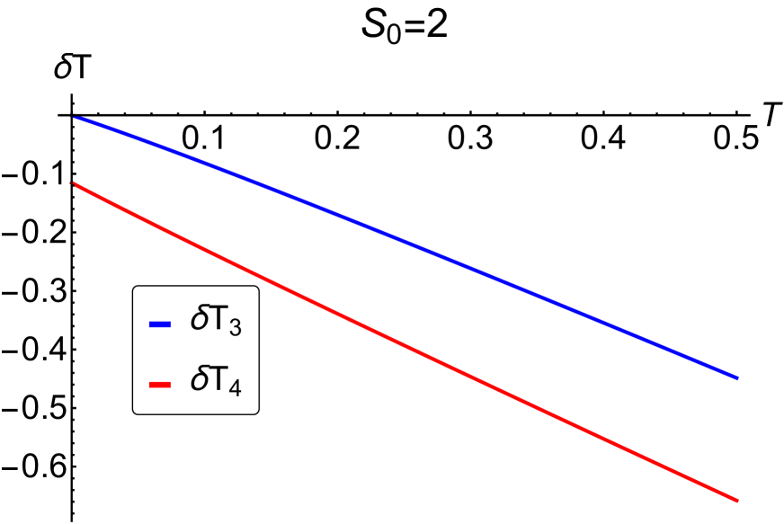
(a) Fixed Entropy

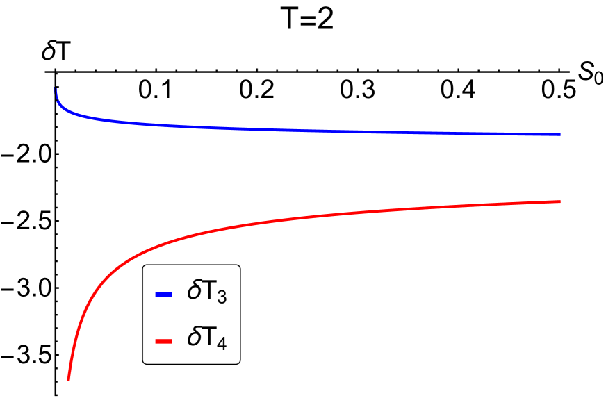
(b) Fixed temperature

Figure 1: Showing the two negative roots of (3.16)

Fig. 1 shows that both $\delta T_{3}$ and $\delta T_{4}$ are real and negative, as discussed. On the other hand, the Freudenthal dual black hole temperature $T+\delta T$ is positive only for $\delta T_{3}$, as shown in Fig. 2. In each figure, we plot two cases, namely when considering fixed entropy $S_{0}$ and when considering fixed temperature $T$.

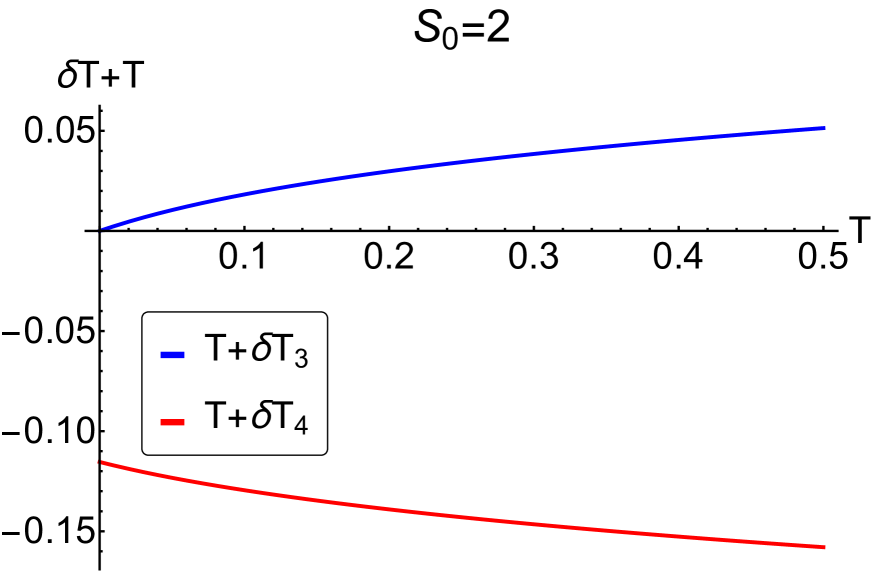
(a) Fixed Entropy

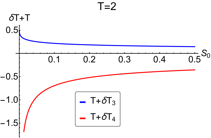
(b) Fixed temperature

Figure 2: Showing the Freudenthal dual temperature $T+\delta T$ corresponding to the two negative real roots $\delta T_{3}$ and $\delta T_{4}$ of (3.16)

Thus, we have finally determined the near-extremal Freudenthal transformation (3.28) for $\delta T=\delta T_{3}\equiv f_{3}\left(T,A\right)$ which satisfies (3.29). This non-linear transformation of the e.m. charges $\mathcal{Q}$ and of the (small) temperature $T$ of a given near-extremal (asymptotically flat, static, spherically symmetric) black hole maps it to another near-extremal (asymptotically flat, static, spherically symmetric) with Freudenthal dual e.m. charges $\mathfrak{F}_{T+\delta T_{3}}\left(\mathcal{Q}\right)$ and Freudenthal dual temperature $T+\delta T_{3}$, but with the same entropy, namely, it holds

$$\mathfrak{F}_{T+\delta T_{3}}\left(S_{NE}\left(\mathcal{Q};T+\delta T_{3}\right)\right)=S_{NE}(\mathcal{Q};T).$$ (3.62)

In other words, we have precisely selected $i=3$ in Eqs. (3.28) and (3.29), disregarding the other three values $i=1,2$ and $4$ (within the labelling defined by formula (3.19)).

Remark

It is here worth remarking that the near-extremal (on-shell) Freudenthal duality $\mathfrak{F}$, defined by (3.28) and (3.29) with $i=3$ (cf. (3.62)), cannot determine a transition to and from the extremal limit :

$$\text{near-extremal}\overset{\mathfrak{F}}{\begin{array}[]{c}\nRightarrow\\ \nLeftarrow\end{array}}\text{extremal.}$$ (3.63)

Proof

$\nLeftarrow$

Since the $\delta T$ pertaining to $\mathfrak{F}$ (i.e., uniquely satisfying (3.16) and (3.31)) is negative, $-T<\delta T<0$, it follows that $\mathfrak{F}$ cannot be used to make a transition from the extremal state ($T=0$) to a near-extremal one ($T>0$), and keep the Bekenstein-Hawking entropy/area of the horizon fixed. In other words, the following transformation :

$$\left\{\begin{array}[]{l}\mathcal{Q}\longrightarrow\mathfrak{F}_{\delta T}\left(\mathcal{Q}\right)\equiv\hat{\mathcal{Q}}\left(\mathcal{Q};\delta T\right):=\Omega\frac{\partial S_{NE}(\mathcal{Q};\delta T)}{\partial\mathcal{Q}};\\ \nobreak\leavevmode\\ T=0\longrightarrow T=\delta T,\end{array}\right.\leavevmode\nobreak\ \text{such\leavevmode\nobreak\ that\leavevmode\nobreak\ }S_{0}\left(\mathcal{Q}\right)=S_{\delta T}\left(\hat{\mathcal{Q}}\left(\mathcal{Q};\delta T\right)\right),$$ (3.64)

cannot occur, simply because $\delta T<0$.

$\nRightarrow$

On the other hand, it can be proved per absurdum that the same $\delta T$ cannot reach the limit value of $-T$. In fact, if we set $\delta T=-T$, one could perform a $\mathfrak{F}$-transformation from a near-extremal state ($T\neq 0$) to the extremal state ($T=0$), and keep the black hole entropy fixed,but this is impossible. In other words, by recalling the definition (3.2), the following transformation :

$$\left\{\begin{array}[]{l}\mathcal{Q}\longrightarrow\mathfrak{F}_{0}\left(\mathcal{Q}\right):=\Omega\frac{\partial S_{0}(\mathcal{Q})}{\partial\mathcal{Q}};\\ \nobreak\leavevmode\\ T\longrightarrow T+\delta T=0,\end{array}\right.\leavevmode\nobreak\ \text{such\leavevmode\nobreak\ that\leavevmode\nobreak\ }S_{NE}\left(\mathcal{Q};T\right)=S_{0}\left(\mathfrak{F}_{0}\left(\mathcal{Q}\right)\right)=S_{0}\left(\mathcal{Q}\right),$$ (3.65)

cannot occur, because, through (2.34), it would imply

$$S_{NE}\left(\mathcal{Q};T\right)\simeq S_{0}\left(\mathcal{Q}\right)+\delta S\left(\mathcal{Q};T\right)=S_{0}\left(\mathcal{Q}\right)$$ (3.66)

$$\Updownarrow$$

$$\delta S\left(\mathcal{Q};T\right)\simeq 0,$$ (3.67)

This cannot true, since, again by means of (2.34), it would yield to

$$TS_{0}\left(\mathcal{Q}\right)=0,$$ (3.68)

which is impossible, because $T>0$ and $S_{0}\left(\mathcal{Q}\right)>0$ $\blacksquare$

4 An Example: STU black hole

In this section, we apply the notion of generalized Freudenthal duality introduced above to deal with an explicit example. Namely, we consider the $STU$ black hole with $D0-D2-D4-D6$ brane charges. The entropy of an extremal black hole with such charge configuration has the following form ($a=1,2,3$) [30],

$$S_{0}=\frac{\pi}{3p^{0}}\sqrt{\frac{4}{3}(\Delta_{a}\tilde{x}^{a})^{2}-9(p^{0}p\cdot q-2D)^{2}}$$

where $q_{0},q_{a},p^{a},p^{0}$ are the $D0,D2,D4$ and $D6$ brane charges respectively, $p\cdot q=p^{0}q_{0}+p^{a}q_{a}$, with $\tilde{x}^{a}$ denoting the real solution of the algebraic inhomogeneous system $\Delta_{a}=D_{abc}\tilde{x}^{b}\tilde{x}^{c}=3D_{a}-p^{0}q_{a}$, and $D_{a}=D_{abc}\,p^{b}p^{c}$, $D=D_{a}p^{a}$. Considering an Ansatz that $\tilde{x}^{a}=\sqrt{{\frac{3D-p^{0}\,q_{b}p^{b}}{D}}}p^{a}$ [22], the extremal entropy can be written as [16],

$$S_{0}={\frac{\pi}{3p^{0}}}\sqrt{{\frac{4}{3}}{\frac{(3D-p^{0}\,q_{a}p^{a})^{3}}{D}}-9(p^{0}\,p\cdot q-2D)^{2}}.$$ (4.1)

Here we begin with an extremal $D0-D2-D4-D6$ STU black hole with charge vectors as $\left(q_{0},q_{a}\right)=(11,5,3,-6)$ and $\left(p^{0},p^{a}\right)=(7,1,2,9)$. The numerical value of the entropy (4.1) of this black hole is $S_{0}=259.534$. As it is an extremal black hole, it has an F-dual with the same value of the entropy, whose charges can be obtained following (2.27) and they are given by $\left(\tilde{q}_{0},\tilde{q}_{a}\right)=(-3.86709,17.0006,7.78631,11.2499)$ and $\left(\tilde{p}^{0},\tilde{p}^{a}\right)=(0.266305,1.42794,2.85587,12.8514)$.

Now we will show numerically that there also exists a unique near-extremal, generalised F-dual black hole to another near-extremal black hole, but with different temperatures. Again, we begin with a $D0-D2-D4-D6$ STU black hole with charge vector $\left(q_{0},q_{a}\right)=(11,5,3,-6)$ and $\left(p^{0},p^{a}\right)=(7,1,2,9)$, and with temperature $T=10^{-3}$ (${{}^{\circ}}K$). Inserting these values to derive the entropy of the corresponding near-extremal black hole, we get the entropy $S_{NE}=289.177$. Following the formulæ discussed in this paper, we find the F-dual charges as

$$\left(\tilde{q}_{0},\tilde{q}_{a}\right) = (-4.02524,17.6959,8.10476,11.71);$$ (4.2)

$$\left(p^{0},p^{a}\right) = (0.277196,1.48634,2.97267,13.377),$$ (4.3)

and the F-dual temperature becomes $T+\delta T=0.000238713$ (${{}^{\circ}}K$). Using these charges and temperature, we find the near-extremal entropy $\tilde{S}_{NE}=289.177$, which is the same as that of the different near-extremal black hole, which we have started with.

5 Conclusion

In this paper, we have introduced the notion of Freudenthal duality for near-extremal black holes, for which the formula (3.1), obtained in [22], holds true. We have explicitly proved that in any four-dimensional Maxwell-Einstein theory with action (2.1) (corresponding to the purely bosonic sector of any $\mathcal{N}\geqslant 2$-extended, $D=4$ supergravity theory), two near-extremal black holes with temperatures respectively $T$ and $T+\delta T$, and with charges related by the Freudenthal duality generated by the near-extremal entropy, can have the same entropy (for a given - unique! - analytical expression of $\delta T$ as a the function of $T$ and of the extremal entropy of one of the two black holes). We have called this duality map, which non-linearly transforms both the e.m. charges and the temperature, near-extremal Freudenthal duality.

It should be remarked that, even if in our treatment we have considered doubly-extremal black holes for simplicity’s sake, our analysis and the resulting Eq. (2.26) are actually holding true for any “large”, asymptotically flat, static, spherically symmetric, dyonic near-extremal black hole in (not necessarily supersymmetric) Einstein-Maxwell-scalar ungauged theories, endowed with a geometry of the scalar manifold such that the e.m. charges under consideration support an attractor solution at the event horizon (in the extremal limit $T\rightarrow 0^{+}$). This is due to the fact that our analysis is strictly confined within the near-horizon region, in which (when assuming the Attractor Mechanism to occur, up to flat directions; cf. footnote 2) the scalar fields are fixed in terms of e.m. charges for any extremal black hole.

Moreover, we would like to stress that temperature is not a fundamental variable: it can always be expressed in terms of the conserved charges of the black hole and the asymptotic values of the scalars. Thus, the transformation under Freudenthal duality of the temperature ${T}$ should be consistent with the transformations of those parameters. In fact, non-extremal black hole do not generally exhibit the Attractor Mechanism, so their Bekenstein-Hawking entropy depends on both the conserved charges of the system (i.e., in the case under consideration, on the e.m. charges) and on the values of the scalar fields at spacial infinity which, in ungauged theories, can be freely specified. Within the framework considered in the present paper, the dependence of temperature on the e.m. charges as well as on the asymptotic values of scalar fields could be obtained as follows : by considering the general expression of the non-extremal black hole entropy, one should expand into the non-extremality parameter, and truncate to the lowest non-trivial order in such a parameter; hence, the comparison with Eqs. (2.26) or (2.34) would allow to obtain the explicit expression of the temperature $T$ in the near-extremal limit in terms of the e.m. charges and of the asymptotic values of scalars. While we consider this task of utmost interest, our humble opinion is that its thorough investigation lies beyond the scope of this paper, in which we have dealt with non-extremality in an effective way, by resorting to temperature within the JT framework.

So far, Freudenthal duality had been introduced for extremal black holes only, in both gauged and ungauged supergravity in four space-time dimensions. Away from extremality (even when the departure from extremality is slight, such as in near-extremal black holes), entropy generally is no more homogeneous of degree two in e.m. charges, and a naïve extension of Freudenthal duality fails. In order to consistently formulate a Freudenthal duality map for near-extremal black holes, we have introduced a (non-linear) transformation of the temperature, as well. By exploiting Descartes’ rule of signs as well as Sturm’s Theorem, which are excellent tools for analysing the real roots of an algebraic equation without solving it, we have precisely shown that for a given set of e.m. charges (which support an extremal black hole with a non-vanishing area of the event horizon and thus with a non-vanishing Bekenstein-Hawking entropy), there indeed exist two near-extremal black holes with two unique, small temperatures such that they share the same entropy while their e.m. charges are related by the Freudenthal duality generated at a non-vanishing temperature. Thus, our analysis sheds new light on the invariance properties of the macroscopic entropy of near-extremal black holes in four space-time dimensions, providing the first example, as far as we know, of intrinsically non-linear symmetry of the entropy itself.

In this paper, we have investigated Freudenthal duality for near-extremal black holes in ungauged supergravity (or, more in general, in absence of a potential for scalar fields and of gauging of the isometries of the associated non-linear sigma model). It would be interesting to extend our analysis to near-extremal black holes in gauged supergravity (or, more in general, in presence of a potential for scalar fields and of gauging of the isometries of the associated non-linear sigma model).

Moreover, in the present work, we did not consider the extra, logarithmic correction to the entropy of near-extremal black holes, which was partially present in the analysis of [22], and which was discussed in its (one-loop) full-fledged form recently in [33]. It would be interesting to analyze the notion of Freudenthal duality for the logarithmic corrected entropy of both extremal and near-extremal black holes. Also, rotating extremal black holes have a Bekenstein-Hawking entropy which is not invariant under the naïvely defined Freudenthal duality, and it would be of interest to investigate the possibility of a consistent generalization of such an intrinsically non-linear map to this class of solutions of the Maxwell-Einstein equations, as well.

It is here worth remarking that in [14] an alternative version of Freudenthal duality was put forward, relying on the crucial observation that the representation of black hole solutions in terms of the $H$-variables (which are harmonic functions in the supersymmetric case) is non-unique, due to the existence of a local symmetry in the effective action. In [14] this symmetry is considered as a continuous (and local) generalization of the Freudenthal duality, which allows to rewrite the physical fields of a solution in terms of entirely different-looking functions. While we agree that the near-horizon limit of the treament of [14] for near-extremal black holes would yield to results consistent with the ones obtained within our investigation, we feel that a thorough study of such a relation would deserve a separate study, which we leave for future work.

Acknowledgments

The work of AC is supported in part by the South African Research Chairs Initiative of the National Research Foundation, grant number 78554 and by the European Union’s Horizon 2020 research and innovation programme under the Marie Sklodowska Curie grant agreement number 101034383.  The work of TM is supported by a Simons Foundation Grant Award ID 509116 and by the South African Research Chairs initiative of the Department of Science and Technology and the National Research Foundation. The work of AM is supported by a “Maria Zambrano” distinguished researcher fellowship at the University of Murcia, Spain, financed by the European Union within the NextGenerationEU programme.

Appendix A Descartes’ rule of signs

Descartes’ rule of signs states that, for a univariate polynomial function $f(x)$ and the corresponding equation

$$f(x)=0,$$ (A.1)

• the number of positive real roots of Eq. (A.1) is the same as (or less than by an even number) the number of changes in the sign of the coefficients of $f(x)$;

• the number of negative real roots of Eq. (A.1) is the same as (or less than by an even number) the number of changes in the sign of the coefficients of $f(-x)$.

Such a rule can be applied to the various cases within the present paper, namely:

1. $$f(x)=x^{3}+2x^{2}+2x+\frac{8}{9}.$$ (A.2)

   Eq. (A.2), which is Eq. (3.8), admits no real positive roots. Since $f(-x)=-x^{3}+2x^{2}-2x+\frac{8}{9}$, Eq. (3.8) admits three or one real negative root(s).

2. $$f(x)=x^{4}+a_{3}x^{3}+a_{2}x^{2}+a_{1}x+a_{0},$$ (A.3)

   with $a_{3},a_{2},a_{1},a_{0}\in\mathbb{R}_{0}^{+}$ . Eq. (A.3), which is Eq. (3.16) with $x\equiv\delta T$ and all the coefficients positive and defined by (3.17), admits no real positive roots. Since $f(-x)=x^{4}-a_{3}x^{3}+a_{2}x^{2}-a_{1}x+a_{0}$, Eq. (3.16) admits four, two or zero real negative roots.

3. $$f(x)=x^{3}-a_{2}x^{2}+\left(a_{1}a_{3}-4a_{0}\right)x+\left(4a_{0}a_{2}-a_{1}^{2}-a_{0}a_{3}^{2}\right),$$ (A.4)

   again with $a_{3},a_{2},a_{1},a_{0}\in\mathbb{R}_{0}^{+}$. From (3.17), since $a_{2}>0$, $a_{1}a_{3}-4a_{0}>0$ and $4a_{0}a_{2}-a_{1}^{2}-a_{0}a_{3}^{2}<0$, Eq. (A.4), which is Eq. (3.27) with $x\equiv y$ and the coefficients defined by (3.17), admits three or one real positive root(s). Since $f(-x)=-x^{3}-a_{2}x^{2}-\left(a_{1}a_{3}-4a_{0}\right)x+\left(4a_{0}a_{2}-a_{1}^{2}-a_{0}a_{3}^{2}\right)$, Eq. (3.27) admits zero real negative roots.

4. $$f(x)=x^{3}+{\frac{1}{16\pi S_{0}}}x^{2}+{\frac{\left(37+128\sqrt{\pi S_{0}}T\right)}{6912\pi^{2}S_{0}^{2}}}x-{\frac{25}{2985984\pi^{3}S_{0}^{3}}}.$$ (A.5)

   Eq. (A.5), which is Eq. (3.55) with $x\equiv y^{\prime}$, admits one real positive root. Since $f(-x)=-x^{3}+{\frac{1}{16\pi S_{0}}}x^{2}-{\frac{\left(37+128\sqrt{\pi S_{0}}T\right)}{6912\pi^{2}S_{0}^{2}}}x-{\frac{25}{2985984\pi^{3}S_{0}^{3}}}$, Eq. (3.55) admits two or zero real negative roots.

Appendix B Sturm’s Theorem

Sturm’s Theorem provides an algorithmic way of calculating the number of simple roots of a non-zero polynomial

$$p(x):=a_{n}x^{n}+a_{n-1}x^{n-1}+\cdots+a_{1}x+a_{0}$$ (B.1)

of degree $n\geqslant 0$ with real coefficients. Before stating Sturm’s Theorem [34, 35, 36], let us introduce the following

Definition

The canonical sequence associated to a non-zero polynomial $p(x)$ is defined as the set of polynomials starting from $p(x)$, with the properties that

1. If $p_{0}(x)=p(x)$ is a constant polynomial, then the sequence stops there.

2. $p_{1}(x)=p^{\prime}(x)$.

3. for $i\geqslant 2$, $p_{i}(x)=-$Rem$(p_{i-2}(x),p_{i-1}(x))$ iff Rem$(p_{i-2}(x),p_{i-1}(x))\neq 0$.
   For non-zero polynomials $a(x)$ and $b(x)$, we denote by Rem$(a(x),b(x))$ the remainder of the Euclidean division of $a(x)$ by $b(x)$.

4. If Rem$(p_{i-2}(x),p_{i-1}(x))=0$, then $p_{i}(x)$ remains undefined, and the sequence stops there.

There are several consequences of the above definition, but one should note that canonical sequence starting with $p_{0}(x)$ always stops in less than $n$ steps, where $n$ is the degree of $p_{0}(x)$; if the last term in the sequence is $p_{m}(x)$, with of course $m\leqslant n$, then $p_{m}(x)$ is equal to the greatest common divisor (gcd) of $p(x)$ and $p^{\prime}(x)$, up to sign.

Definition

Let $p_{0}(x),p_{1}(x),\cdots,p_{m}(x)$ be a non-empty finite sequence of polynomials, with $p_{0}(x)$ not identically zero. Such a sequence is called a Sturm sequence iff

1. The last term $p_{m}(x)$ of the sequence is either always positive or always negative on the real line.

2. No two consecutive $p_{i}(x)$ are simultaneously zero for $x$ a real number.

3. Suppose that $\alpha$ is a root of $p_{i}(x)$, for some $i$ with $0<i<m$. Then $p_{i-1}(\alpha)$ and $p_{i+1}(\alpha)$ have opposite signs.

4. At any real root $\alpha$ of $p_{0}(x)$, the values of $p_{0}(x)$ at $\alpha+0$ and $\alpha-0$ is of opposite sign. This last condition ensures that $\alpha$ cannot be a repeated root of $p_{0}(x)$.

One can prove that the canonical sequence associated to a polynomial without repeated real roots is a Sturm sequence.

The final ingredient that we need to state Sturm’s Theorem is the sign change number function. Given $\alpha\in\mathbb{R}$ and a polynomial $p(x)$, the number of sign change function at $\alpha$, denoted by $\sigma(\alpha)$, as the number of sign changes (ignoring the zeros) in any Sturm sequence associated to $p(x)$, computed at $x=\alpha$.

We can now state

Sturm’s Theorem

Let $p(x)$ be a non-zero polynomial with real coefficients. The number of distinct real roots (counted without multiplicity) of $p(x)$ in an interval $(a,b]$ of the real line is given by $\sigma(a)-\sigma(b)$, the difference in the sign change number function at the end points $a$ and $b$, with respect to any Sturm sequence associated to the given polynomial $p(x)$.

When we are interested in looking for real roots of a polynomial $p(x)$ (without repeated real roots) in a given interval of the real line, we can construct the canonical sequence associated to $p(x)$ (which will be a Sturm sequence associated to $p(x)$ itself), and calculate the difference between the values of the sign change number function of $p(x)$ evaluated at the extrema of the interval, in order to determine the number of real roots of $p(x)$ in such an interval. On the other hand, Descartes’ rule of signs applied to $p(x)$ will let us know about the number of roots being on the positive or negative part of the real axis.

Example I

Let us consider Eq. (3.8). The canonical sequence associated to

$$p_{0}(x):=x^{3}+2x^{2}+2x+\frac{8}{9},$$ (B.2)

which in this case is a Sturm sequence associated to $p_{0}(x)$ itself, is given by

$$\begin{split}p_{0}(x)&=x^{3}+2x^{2}+2x+{\frac{8}{9};}\\ p_{1}(x)&=2+4x+3x^{2};\\ p_{2}(x)&=-{\frac{4}{9}}(1+x);\\ p_{3}(x)&=-1.\end{split}$$ (B.3)

We want to calculate the number of real roots of the polynomial $p_{0}(x)$, namely the number of real roots in the interval $(-\infty,\infty)$. Therefore we check the sign changes for this sequence at $-\infty$ and $\infty$. We find that at $x=-\infty$,

$p_{0}$	$p_{1}$	$p_{2}$	$p_{3}$
-	+	+	-

Thus, $\sigma(-\infty)=2$. Similarly at $x=\infty$, we find

$p_{0}$	$p_{1}$	$p_{2}$	$p_{3}$
+	+	-	-

implying $\sigma(\infty)=1$. This yields

$$\sigma(-\infty)-\sigma(\infty)=2-1=1,$$ (B.4)

signalling the existence of a single real root between $(-\infty,\infty)$. Either using Descartes’ rule of signs, or by splitting the interval $(-\infty,\infty)$ in positive and negative semilines and applying Sturm’s Theorem twice, one can finally prove that Eq. (3.8) admits only one real root, which is negative.

Example II

Let us consider Eq. (3.27). By considering $a_{0},a_{1},a_{2},a_{3}$ $\in\mathbb{R}_{0}^{+}$ and $B\in\mathbb{R}_{0}^{-}$, the canonical sequence associated to

$$p_{0}\left(y\right):=y^{3}-a_{2}y^{2}+(a_{1}a_{3}-4a_{0})y+B,$$ (B.5)

which in this case is a Sturm sequence associated to $p_{0}(y)$ itself, is given by

$$p_{0}(y) = y^{3}-a_{2}y^{2}+\left(a_{1}a_{3}-4a_{0}\right)y+B;$$

$$p_{1}(y) = 3y^{2}-2a_{2}y+B_{1};$$

$$p_{2}(y) = B_{2}y+B_{3};$$

$$p_{3}(y) = 4a_{0}-a_{1}a_{3}+{\frac{1}{B_{2}^{2}}}\left({\frac{64}{3}}a_{0}a_{1}^{2}a_{2}-{3a_{1}^{4}}-{\frac{1024}{27}}a_{0}^{2}a_{2}^{2}+{\frac{2}{3}}a_{1}^{3}a_{2}a_{3}-{\frac{64}{27}}a_{0}a_{1}a_{2}^{2}a_{3}\right.$$ (B.6)

$$-6a_{0}a_{1}^{2}a_{3}^{2}+{\frac{64}{3}}a_{0}^{2}a_{2}a_{3}^{2}-{\frac{1}{27}}a_{1}^{2}a_{2}^{2}a_{3}^{2}+{\frac{2}{3}}a_{0}a_{1}a_{2}a_{3}^{3}-3a_{0}^{2}a_{3}^{4}-2B_{2}a_{1}^{2}a_{2}$$

$$\left.+{\frac{64}{9}}B_{2}a_{0}a_{2}^{2}+{\frac{2}{9}}B_{2}a_{1}a_{2}^{2}a_{3}-2B_{2}a_{0}a_{2}a_{3}^{2}\right),$$

where, by setting

$$B:=4a_{0}a_{2}-a_{1}^{2}-a_{0}a_{3}^{2},$$ (B.7)

it follows that

$$B_{1} : =-4a_{0}+a_{1}a_{3};$$

$$B_{2} : =\frac{8}{3}a_{0}+\frac{2}{9}a_{2}^{2}-\frac{2}{3}a_{1}a_{3};$$

$$B_{3} : =a_{1}^{2}-{\frac{32a_{0}a_{2}}{9}}-{\frac{a_{1}a_{2}a_{3}}{9}}+a_{0}a_{3}^{2}.$$ (B.8)

We want to calculate the sign sequence at the three points $y=\{-\infty,0,\infty\}$. By recalling the definitions (3.17) and the fact that both $S_{0}$ and $T$ are real positive (with $T$ also small), we find the signs of $B,B_{1},B_{2}$ and $B_{3}$ are $\{-,+,-,+\}$, $p_{3}(y)<0$ $\forall y\in\mathbb{R}$. With these information, we find that the signs of the Sturm sequence associated to $p_{0}(y)$ evaluated at $y=\{-\infty,0,\infty\}$ are respectively given by the following quadruplets : $\{-,+,+,-\}$, $\{-,+,+,-\}$, $\{+,+,-,-\}$. Thus, we obtain

$$\sigma(-\infty)=2,\quad\sigma(0)=2,\quad\sigma(\infty)=1,$$ (B.9)

which implies that Eq. (3.27) admits only one real root, which is positive. Therefore, for any positive and real value of $T$ and $S_{0}$, Eq. (3.27) always admits only one real root, which is positive.

Analogously, one can show that the Sturm sequence associated to Eq. (3.55) has exactly the same values of $\sigma(\alpha)$ as the example (B.5), at $\alpha=\{-\infty,0,\infty\}$. This implies that Eq. (3.55) has only one real root, which is positive too.

References

- [1] C. Teitelboim, Gravitation and Hamiltonian Structure in Two Space-Time Dimensions, Phys. Lett. B 126 (1983) 41–45.
- [2] R. Jackiw, Lower Dimensional Gravity, Nucl. Phys. B 252 (1985) 343–356.
- [3] J. Maldacena, D. Stanford and Z. Yang, Conformal symmetry and its breaking in two dimensional Nearly Anti-de-Sitter space, PTEP 2016 (2016) 12C104, [1606.01857].
- [4] A. Almheiri and J. Polchinski, Models of AdS2 backreaction and holography, JHEP 11 (2015) 014, [1402.6334].
- [5] P. Nayak, A. Shukla, R. M. Soni, S. P. Trivedi and V. Vishal, On the Dynamics of Near-Extremal Black Holes, JHEP 09 (2018) 048, [1802.09547].
- [6] U. Moitra, S. K. Sake, S. P. Trivedi and V. Vishal, Jackiw-Teitelboim Gravity and Rotating Black Holes, JHEP 11 (2019) 047, [1905.10378].
- [7] K. S. Kolekar and K. Narayan, AdS2 dilaton gravity from reductions of some nonrelativistic theories, Phys. Rev. D 98 (2018) 046012, [1803.06827].
- [8] N. Banerjee, T. Mandal, A. Rudra and M. Saha, Equivalence of JT gravity and near-extremal black hole dynamics in higher derivative theory, JHEP 01 (2022) 124, [2110.04272].
- [9] L. Borsten, D. Dahanayake, M. J. Duff and W. Rubens, Black holes admitting a Freudenthal dual, Phys. Rev. D 80 (2009) 026003, [0903.5517].
- [10] S. Ferrara, A. Marrani and A. Yeranyan, Freudenthal Duality and Generalized Special Geometry, Phys. Lett. B 701 (2011) 640–645, [1102.4857].
- [11] L. Borsten, M. J. Duff, S. Ferrara and A. Marrani, Freudenthal Dual Lagrangians, Class. Quant. Grav. 30 (2013) 235003, [1212.3254].
- [12] D. Klemm, A. Marrani, N. Petri and M. Rabbiosi, Nonlinear symmetries of black hole entropy in gauged supergravity, JHEP 04 (2017) 013, [1701.08536].
- [13] A. Marrani, C.-X. Qiu, S.-Y. D. Shih, A. Tagliaferro and B. Zumino, Freudenthal Gauge Theory, JHEP 03 (2013) 132, [1208.0013].
- [14] P. Galli, P. Meessen and T. Ortin, The Freudenthal gauge symmetry of the black holes of N=2,d=4 supergravity, JHEP 05 (2013) 011, [1211.7296].
- [15] J. J. Fernandez-Melgarejo and E. Torrente-Lujan, SUGRA BPS Multi-center solutions, quadratic prepotentials and Freudenthal transformations, JHEP 05 (2014) 081, [1310.4182].
- [16] A. Marrani, P. K. Tripathy and T. Mandal, Supersymmetric Black Holes and Freudenthal Duality, Int. J. Mod. Phys. A 32 (2017) 1750114, [1703.08669].
- [17] L. Borsten, M. J. Duff and A. Marrani, Freudenthal duality and conformal isometries of extremal black holes, 1812.10076.
- [18] L. Borsten, M. J. Duff, J. J. Fernández-Melgarejo, A. Marrani and E. Torrente-Lujan, Black holes and general Freudenthal transformations, JHEP 07 (2019) 070, [1905.00038].
- [19] A. Marrani, Freudenthal Duality in Gravity: from Groups of Type E7 to Pre-Homogeneous Spaces, p Adic Ultra. Anal. Appl. 7 (2015) 322–331, [1509.01031].
- [20] A. Marrani, Non-Linear Invariance of Black Hole Entropy, PoS EPS-HEP2017 (2017) 543.
- [21] A. Marrani, Non-linear Symmetries in Maxwell-Einstein Gravity: From Freudenthal Duality to Pre-homogeneous Vector Spaces, Springer Proc. Math. Stat. 335 (2019) 253–264.
- [22] A. Chattopadhyay and T. Mandal, Freudenthal duality of near-extremal black holes and Jackiw-Teitelboim gravity, Phys. Rev. D 105 (2022) 046014, [2110.05547].
- [23] L. V. Iliesiu and G. J. Turiaci, The statistical mechanics of near-extremal black holes, JHEP 05 (2021) 145, [2003.02860].
- [24] B. Bertotti, Uniform electromagnetic field in the theory of general relativity, Phys. Rev. 116 (1959) 1331.
- [25] I. Robinson, A Solution of the Maxwell-Einstein Equations, Bull. Acad. Pol. Sci. Ser. Sci. Math. Astron. Phys. 7 (1959) 351–352.
- [26] S. Ferrara, G. W. Gibbons and R. Kallosh, Black holes and critical points in moduli space, Nucl. Phys. B 500 (1997) 75–93, [hep-th/9702103].
- [27] S. Ferrara, R. Kallosh and A. Strominger, N=2 extremal black holes, Phys. Rev. D 52 (1995) R5412–R5416, [hep-th/9508072].
- [28] S. Ferrara and R. Kallosh, Supersymmetry and attractors, Phys. Rev. D 54 (1996) 1514–1524, [hep-th/9602136].
- [29] S. Ferrara and R. Kallosh, Universality of supersymmetric attractors, Phys. Rev. D 54 (1996) 1525–1534, [hep-th/9603090].
- [30] M. Shmakova, Calabi-Yau black holes, Phys. Rev. D 56 (1997) 540–544, [hep-th/9612076].
- [31] S. Ferrara, A. Marrani, E. Orazi and M. Trigiante, Dualities Near the Horizon, JHEP 11 (2013) 056, [1305.2057].
- [32] M. Abramowitz and I. Stegun, eds., Handbook of Mathematical Functions. Dover, New York, 1965.
- [33] L. V. Iliesiu, S. Murthy and G. J. Turiaci, Revisiting the Logarithmic Corrections to the Black Hole Entropy, 2209.13608.
- [34] H. Dörrie and D. Antin, 100 Great Problems of Elementary Mathematics: Their History and Solution. Dover Books on Mathematics Series. Dover Publications, 1965.
- [35] K. N. Raghavan, Sturm’s method for the number of real roots of a real polynomial. "https://www.imsc.res.in/knr/past/sturm/formal_notes.pdf".
- [36] P. Bartlett, Finding All the Roots: Sturm’s Theorem. "http://web.math.ucsb.edu/ padraic/mathcamp_2013/root_find_alg/Mathcamp_2013_Root-Finding_Algorithms_Day_2.pdf".