Spin resonance induced by a mechanical rotation of a polariton condensate

Abstract

We study theoretically the polarization dynamics in a ring-shape bosonic condensate of exciton-polaritons confined in a rotating trap. The interplay between the rotating potential and TE-TM splitting of polariton modes offers a tool of control over the spin state and the angular momentum of the condensate. Specific selection rules describing the coupling of pseudospin and angular momentum are formulated. The resonant coupling between states having linear and circular polarizations leads to the polarization beats. The effect may be seen as a polariton analogy to the electronic magnetic resonance in the presence of constant and rotating magnetic fields. Remarkably, spin beats are induced by a purely mechanical rotation of the condensate.

Introduction. Exciton-polaritons are hybrid light-matter quasiparticles emerging in the regime of the strong coupling between a photonic mode of a planar semiconductor microcavity and an excitonic resonance in a quantum well embedded in the antinode of a cavity mode. From their photonic component polaritons inherit extremely small effective mass (about $10^{-5}$ of the mass of free electrons) and large coherence length (in the mm scale) [1]. On the other hand, the presence of an excitonic component leads to the sensitivity of the polariton systems to external electric and magnetic fields, and robust polartion-polariton interactions [2].

Remarkable tunability of cavity polaritons allows to engineer their spatial confinement in a variety of experimental geometries, ranging from individual micropillars [3, 4, 5, 6] to the systems of several coupled pillars forming so-called polariton molecules [7, 8] or periodically arranged arrays of the pillars forming polariton superlattices [9, 10, 11, 12, 13]. Annular geometries are of particular interest, as in this case the interplay between non-trivial topology of the system and polarization TE-TM and Zeeman splittings can lead to a variety of intriguing physical phenomena, such as formation of the polaritonic persistent currents [14] including symmetry breaking in spinor polariton current states [15], linear [16] and nonlinear [17] polaritonic Aharonov-Bohm effect, topological spin Meissner effect [18], angular momentum fractionalization [19], and others. Moreover, it was recently proposed, that polariton rings can form a material platform for the realization of optical qubits [20].

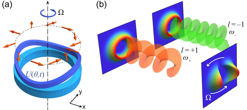
Figure 1: (a) Polariton ring condensate (blue) in the presence of TE-TM splitting, producing an effective magnetic field (orange arrows) acting on pseudospins of polaritons, subjected to an external rotating perturbation potential ${U(\theta,t)=U_{0}\cos(2\theta-\Omega t)}$. Orange arrows indicate the directions of the effective magnetic field produced by the TE-TM splitting along the ring. (b). Superposition of the two Laguerre-Gaussian laser beams characterised by the angular momenta $l=\pm 1$ and slightly different in frequencies $\omega_{\pm}$. The frequency detuning between the two beams leads to the appearance of the angular potential, rotating with the frequency $\Omega=\omega_{+}-\omega_{-}$.

In the present paper we theoretically predict a strong polarization resonance to appear in a ring-shape polariton condensate subject to a rotating potential trap. Such rotating traps can be produced by optical pumping with Laguerre-Gaussian laser beams as detailed below. We demonstrate, that linear to circular polarization coupling provided by the perturbation leads to the strong beats between the corresponding states. The phenomenon is a polaritonic counterpart of the magnetic resonance experienced by the spin of an electron placed in a combination of constant and rotating magnetic fields.

The model. We assume the geometry of an experiment illustrated in Fig. 1(a). A thin polariton ring of the radius $R$, is subjected to the external scalar perturbation potential having the form

$$U(\theta,t)=U_{0}\cos(2\theta-\Omega t),$$ (1)

where $\theta$ is an angular coordinate along the ring.We assume that the thickness of the ring $d\ll R$, so that only the lowest radial mode can be excited. Such kind of a perturbation results from a superposition of two optical Laguerre-Gaussian modes having the angular momenta $l=\pm 1$, which are slightly detuned in energy [21] (see Fig. 1(b)).

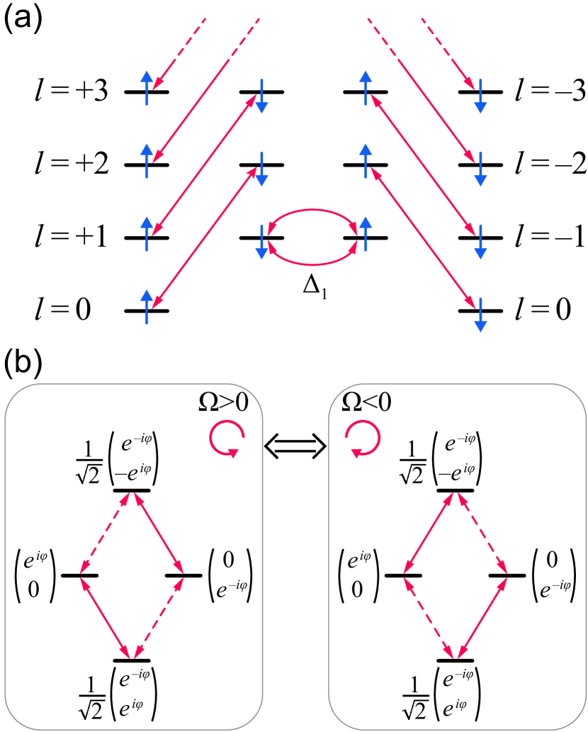
Figure 2: (Color online) (a) Scheme of the coupling of the levels of a polariton ring by TE-TM interaction $\Delta_{1}$ (see Eq. (6)). Black horizontal lines correspond to the energy levels for the case $\Delta_{1}$=0, up and down vertical arrows denote states with right and left circular polarizations, $l$ correspond to the winding numbers. The ground state is twice degenerate in polarization, all other states are four time degenerate: in polarization and sign of $l$. If $\Delta_{1}\neq 0$, the states with $l_{\downarrow}-l_{\uparrow}=2$ become mixed, and degenaracies are partially lifted. Among all coupled pairs, the one corresponding to the states with $l_{\downarrow}=1,l_{\uparrow}=-1$ is particular, as corresponding states have equal energies, and thus they are most efficiently coupled by TE-TM splitting. (b). The scheme illustrating the transitions induced by the rotating potential $U(\theta,t)=U_{0}\cos(2\theta-\Omega t)$ in the subspace of the states with winding numbers $l_{\uparrow,\downarrow}=\pm 1$. Upper and lower states are strongly split due to TE-TM interaction and are linearly polarized in radial and tangential directions, respectively. Two states in the middle remain degenerate in energy and correspond to two circular polarizations. Resonant and anti-resonant transitions are shown by solid and dashed red arrows, respectively.

The state of the system is described by a two component spinor, corresponding to the two opposite circular polarizations $\psi=(\psi_{\uparrow},\psi_{\downarrow})^{\text{T}}$, and its dynamics is given by a Shrödinger-type equation,

$$i\hbar\partial_{t}\psi=\hat{H}\psi.$$ (2)

In this paper, we focus on the conservative linear limit, where we neglect the dissipative nature of cavity polaritons and polariton-polariton interactions. These approximations will allow us to reveal the proposed effect analytically. We acknowledge that the optical pump in polariton systems normally crates a complex potential whose imaginary part corresponds to the effective gain seen by the polaritons, but related effects require special consideration which is left for the follow-up paper. In the same time we would like to emphasise that the conservative case is also very relevant from physical point of view.

The operator $\hat{H}$ in this approximation is hermitian and corresponds to the Hamiltonian of the system, which reads [22]:

$$\hat{H}=\hat{H}_{0}+U(\theta,t),$$ (3)

where, in the basis of the circular polarizations

$$\hat{H}_{0}=\frac{\hbar^{2}}{2m_{p}R^{2}}\left(\begin{array}[]{cc}-\partial_{\theta}^{2}&\Delta_{1}e^{-2i\theta}\\ \Delta_{1}e^{2i\theta}&-\partial_{\theta}^{2}\end{array}\right).$$ (6)

Here $m_{p}$ is an effective mass of polaritons, $\partial_{\theta}=d/d\theta$, and the dimensionless parameter $\Delta_{1}$ is proportional to the inverse square of the ring thickness $d$ and characterizes the value of the TE-TM splitting in the system.

To better understand the effect proposed here qualitatively, let us first consider the structure of the energy levels of a ring described by the Hamiltonian (6). In the case where TE-TM splitting is absent ($\Delta_{1}=0$), the states of the opposite circular polarizations are decoupled from each other, so that the energy levels are characterized by the independent winding numbers $l_{\uparrow}$ and $l_{\downarrow}$, corresponding to right and left circular polarizations, respectively. The ground state with $l_{\uparrow}=l_{\downarrow}=0$ is twice degenerated, while all upper energy levels are degenerated four times, as clockwise and anticlockwise rotations, corresponding to the different signs of $l$ are all equivalent.

The presence of the TE-TM splitting mixes the states with opposite circular polarizations having the winding numbers $l_{-}-l_{+}=2$, as it is shown by the red arrows in Fig. 2(a). One can see that the states with $l_{\pm}=\pm 1$ are different from all the rest [23], as only within this quadruplet we have a pair of the states with the same energy coupled to each other. We will therefore focus on them and project the dynamic equation (2) into the corresponding subspace. Its four basis vectors split in the two groups.

The first one corresponds to the states with ${l_{\uparrow}=-1}$, ${l_{\downarrow}=+1}$, coupled by TE-TM splitting. As the result, two linearly polarized states, with tangential and radial polarizations are produced, with the energies ${E_{T}=\hbar^{2}(1-\Delta_{1})/2m_{p}R^{2}}$ and ${E_{R}=\hbar^{2}(1+\Delta_{1})/2m_{p}R^{2}}$ and wave functions

$$\psi_{T}=\frac{1}{\sqrt{2}}\left(\begin{array}[]{c}e^{-i\theta}\\ e^{i\theta}\end{array}\right),\psi_{R}=\frac{1}{\sqrt{2}}\left(\begin{array}[]{c}e^{-i\theta}\\ -e^{i\theta}\end{array}\right).$$ (11)

The second group corresponds to a pair of degenerate states, which stem from the states with ${l_{\uparrow}=+1}$ and ${l_{\downarrow}=-1}$, with some admixture of the states with $l_{\uparrow}=-3,l_{\downarrow}=3$. For simplicity, we neglect this admixture, assuming that ${\Delta_{1}\ll 1}$. In this case, these states remain circularly polarized, their energies being ${E_{c}=\hbar^{2}/2m_{p}R^{2}}$ and the wave functions

$$\psi_{\uparrow}=\left(\begin{array}[]{c}e^{i\theta}\\ 0\end{array}\right),\psi_{\downarrow}=\left(\begin{array}[]{c}0\\ e^{-i\theta}\end{array}\right).$$ (16)

Approximating the wavefunction as $\psi=\sum_{j}A_{j}\psi_{j}$, where $j=T,R,\uparrow,\downarrow$ we obtain the following set of the coupled equations for the amplitudes of the modes $A_{j}$:

$$\partial_{t}A_{T}=-i\omega_{c}(1-\Delta_{1})A_{T}+i\eta\left(e^{i\Omega t}A_{\uparrow}+e^{-i\Omega t}A_{\downarrow}\right),\,$$ (17a)

$$\partial_{t}A_{R}=-i\omega_{c}(1+\Delta_{1})A_{R}+i\eta\left(e^{i\Omega t}A_{\uparrow}-e^{-i\Omega t}A_{\downarrow}\right),\,$$ (17b)

$$\partial_{t}A_{\uparrow}=-i\omega_{c}A_{\uparrow}+i\eta e^{-i\Omega t}(A_{T}+A_{R}),\,$$ (17c)

$$\partial_{t}A_{\downarrow}=-i\omega_{c}A_{\downarrow}+i\eta e^{i\Omega t}(A_{T}-A_{R}),\,$$ (17d)

where $\omega_{c}=E_{c}/\hbar,\eta=U_{0}/\hbar$. As one can see, the rotating perturbation mixes the states with linear and circular polarizations, while it does not mix the states of the opposite linear polarizations $A_{R}$ and $A_{T}$ directly. This is because of the interplay between TE-TM splitting and particular symmetry of the perturbation, which mixes the components with the winding numbers differing by two.

Rotating wave approximation. Let us consider the resonant case, where $\Omega\approx\omega_{c}\Delta_{1}$. One can see that the couplings can be either resonant, or antiresonant, depending on the sign of $\Omega$, i.e. the direction of the rotation of the perturbation. In the case, when $\Omega>0$ the tangentially linearly polarized lowest energy state resonantly couples to the right circular polarized state, and antiresonantly to the left circular polarized state, while the radially polarized highest energy state, on the contrary, resonantly couples to the left circular polarized state, and antiresonantly to the right circular polarized state. The change of the rotation direction will lead to the inversion of the coupling scheme, as it is shown in Fig. 2(b).

In the rotating wave approximation the system of the four coupled equations thus splits into the two independent pairs, each of which coincides with well known equations for the description of the magnetic resonance of a spin,

$$\partial_{t}A_{T}=-i\omega_{c}(1-\Delta_{1})A_{T}+i\eta e^{i\Omega t}A_{\uparrow},$$ (18a)

$$\partial_{t}A_{\uparrow}=-i\omega_{c}A_{\uparrow}+i\eta e^{-i\Omega t}A_{T},$$ (18b)

and

$$\partial_{t}A_{R}=-i\omega_{c}(1+\Delta_{1})A_{R}-i\eta e^{-i\Omega t}A_{\downarrow},$$ (19a)

$$\partial_{t}A_{\downarrow}=-i\omega_{c}A_{\downarrow}-i\eta e^{i\Omega t}A_{R}.$$ (19b)

The application of the resonant rotating perturbation will thus lead to linear-circular polarization beats. Note, that for a stationary potential ($\Omega=0$), two circular polarized components will be coupled instead [24].

In resonant approximation one can easily get the simple analytical expression for the polarization occupancies. For example, if at $t=0$ the lowest energy linear polarized state $A_{T}$ is populated, the occupancy of the circular polarized state resonantly coupled to it is

$$|A_{\uparrow}(t)|^{2}|=\frac{4\eta^{2}}{4\eta^{2}+\delta^{2}}\sin^{2}\left(\sqrt{\frac{\delta^{2}}{4}+\eta^{2}}t\right),$$ (20)

where $\delta=\Omega-\omega_{c}\Delta_{1}$ is the detuning from the exact resonance [24].

The temporal evolution of the resonant $A_{T,\uparrow}(t)$ and nonresonant $A_{R,\downarrow}(t)$ modes calculated from (17) is illustrated in Figs. 3(a) and 3(b), respectively. One can see that the contribution of the nonresonant modes is negligibly small, and the formula (20) gives almost perfect approximation of the systems dynamics.

The normalized Stokes vectors $\vec{S}=(\psi^{\dagger}\vec{\sigma}\psi)/\psi^{\dagger}\psi$ accompanied by polariztion ellipses at different spatial points are shown in panels (c)–(e) and (f)–(h), respectively, for the times corresponding to the maximum occupancy of $A_{T}$ states, the maximum occupancy of $A_{\uparrow}$ state and the moment when these modes have the same occupancies. $\vec{\sigma}=(\sigma_{1},\sigma_{2},\sigma_{3})$ is the vector of Pauli matrices. One can clearly see the beatings between linear and circular polarized states, going through elliptically polarized states at intermediate times.

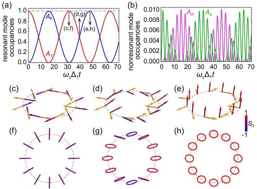
Figure 3: (Color online) The dependencies of the occupancies of the resonant $A_{T,\uparrow}$ (a) and nonresonant $A_{R,\downarrow}$ (b) modes on time for the case of the exact resonance, $\omega_{c}\Delta_{1}=\Omega$. The normalized Stokes vector $\vec{S}$ and the effective magnetic field at different angular positions on the ring are shown in panels (c)–(e) for the times indicated in (a). The arrows showing the Stokes vector are shown in color ranging from red to blue. Orange arrows indicate the orientation of the effective magnetic field. The polarization ellipses are shown in panels (f)–(h). The parameters are ${\omega_{c}\Delta_{1}=\Omega=1}$, ${\eta=0.1}$.

Floquet spectrum. The coefficients in the system (17) are periodic functions of time, and, according to the Floquet theorem the solutions of the system can be resperentes in the form

$$A_{j}(t)=e^{-i\varepsilon t/\hbar}a_{j}(t),$$ (21)

where $a_{j}(t)=a_{j}(t+2\pi/\Omega)$ are periodic functions of time. The parameters $\varepsilon$ correspond to the so-called Floquet quasienergies of the system [25].

In our case, making the substitution $(a_{1},a_{2},a_{2},a_{4})^{\text{T}}=(b_{1},b_{2},b_{3}e^{-i\Omega t},b_{4}e^{i\Omega t})^{\text{T}}$ we get:

$$i\frac{\partial\vec{b}}{\partial t}=\hat{L}\vec{b},$$ (22)

where the matrix $\hat{L}$ is time independent,

$$\hat{L}=\left(\begin{array}[]{cccc}\omega_{c}(1-\Delta_{1})&0&-\eta&-\eta\\ 0&\omega_{c}(1+\Delta_{1})&-\eta&\eta\\ -\eta&-\eta&\omega_{c}-\Omega&0\\ -\eta&\eta&0&\omega_{c}+\Omega\\ \end{array}\right).\,\,$$ (27)

and Floquet quasienergies, up to a Planck constant, can be thus found as its eigenvalues. Thus we conclude that the problem of polariton states in a rotating potential can be conveniently considered in terms of Floquet states.

Note that Floquet quasienergies can be found analytically, but corresponding expressions are bulky and they are not shown here. Instead we plot in Figure 4 the calculated dependencies of the Floquet energies on the rotation velocity $\Omega$. The presence of the rotating potential leads to the visible anticrossings of the Floquet quasienergies at $\Omega=0$ and $\Omega=\pm\omega_{c}\Delta_{1}$. Around $\Omega=0$ the anticrossing comes from the coupling between the states of the opposite circular polarizations $\psi_{\uparrow}$ and $\psi_{\downarrow}$, while at $\Omega=\pm\omega_{c}\Delta$ – from the coupling between linear and circular polarized states, as it is shown in Fig. 2.

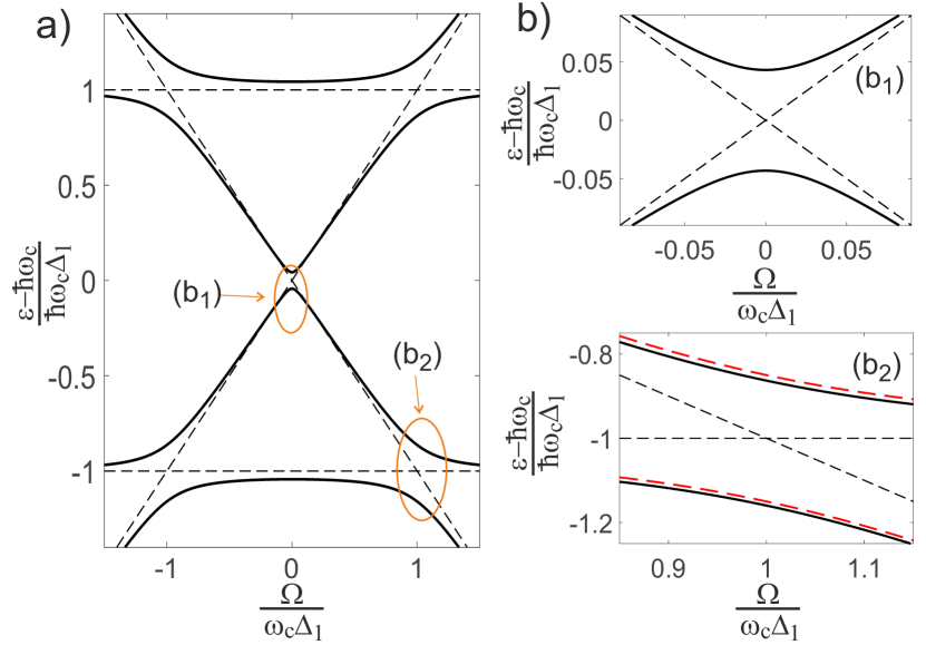
Figure 4: (Color online) The dependencies of the Floquet eigenenergies on the potential rotation velocity $\Omega$ are shown in panel (a) for $\frac{\eta}{\omega_{c}\Delta_{1}}=0.15$. The thin dashed lines correspond to the case $\eta=0$. The panels (b₁) and (b₂) show the energy level splitting in the areas shown by the orange ovals in panel (a). The red lines in the right inset correspond to the eigenenergies calculated neglecting the anti-resonant terms.

Close to the resonance, in the rotating wave approximation Floquet quasienergies can be approximated as  [24]:

$$\varepsilon=\hbar\left(\omega_{c}+\frac{\omega_{c}\Delta_{1}+\Omega}{2}\pm\sqrt{\frac{(\omega_{c}\Delta_{1}-\Omega)^{2}}{4}+\eta^{2}}\right),\qquad\,$$ (28a)

$$\varepsilon=\hbar\left(\omega_{c}-\frac{\omega_{c}\Delta_{1}+\Omega}{2}\pm\sqrt{\frac{(\omega_{c}\Delta_{1}-\Omega)^{2}}{4}+\eta^{2}}\right).\qquad\,$$ (28b)

They are shown by the red lines in panel (b₂). One can see that for a relatively shallow rotating potential the perturbation theory provides a very accurate estimate for the eigenenergies. Note here that the limit of shallow potential is highly relevant to the experiments with optically induced rotating traps  [21].

Conclusions. In conclusion, we predict a parametric resonance leading to the polarization beats in polariton ring condensates subjected to a rotating perturbation. The considered effect is a polaritonic analogue of the electronic magnetic resonance. We demonstrate, that a rotating perturbation leads to the beats between linear and circular polarizations that manifest a cyclic dynamics of the polariton pseudospin. The phenomenon is a remarkable manifestation of the effect of mechanical rotation on spin properties of a quantum object. It may be used as a tool of control over the quantum state of a ring-shape polariton condensate which is important for applications in quantum and classical polariton computing. Finally, let us notice that the incoherent pumping of polariton condensates creates complex effective potentials in general. The imaginary part of such a potential accounting for the interplay between losses and gain in each specific point of the real space. This interplay may lead to the pseudodrag effect  [26] that remained beyond the scope of the present study.

A.V.Y. and I.A.S. acknowledge financial support from Icelandic Research Fund (Rannis, the project “Hybrid polaritonics”), “Priority 2030 Academic Leadership Program” and “Goszadanie no. 2019-1246”. A.V.K. and E.S.S. acknowledge Saint-Petersburg State University for the financial support (research grant No 91182694). E.S.S. acknowledges support from the RF Ministry of Science and Higher Education as part of State Task no. 0635-2020-0013.

References

- Ballarini et al. [2017] D. Ballarini, D. Caputo, C. S. Muñoz, M. De Giorgi, L. Dominici, M. H. Szymańska, K. West, L. N. Pfeiffer, G. Gigli, F. P. Laussy, et al., Phys. Rev. Lett. 118, 215301 (2017), URL https://link.aps.org/doi/10.1103/PhysRevLett.118.215301.
- Glazov et al. [2009] M. M. Glazov, H. Ouerdane, L. Pilozzi, G. Malpuech, A. V. Kavokin, and A. D’Andrea, Phys. Rev. B 80, 155306 (2009), URL https://link.aps.org/doi/10.1103/PhysRevB.80.155306.
- Bajoni et al. [2008] D. Bajoni, P. Senellart, E. Wertz, I. Sagnes, A. Miard, A. Lemaître, and J. Bloch, Phys. Rev. Lett. 100, 047401 (2008), URL https://link.aps.org/doi/10.1103/PhysRevLett.100.047401.
- Ctistis et al. [2010] G. Ctistis, A. Hartsuiker, E. van der Pol, J. Claudon, W. L. Vos, and J.-M. Gérard, Phys. Rev. B 82, 195330 (2010), URL https://link.aps.org/doi/10.1103/PhysRevB.82.195330.
- Ferrier et al. [2011] L. Ferrier, E. Wertz, R. Johne, D. D. Solnyshkov, P. Senellart, I. Sagnes, A. Lemaître, G. Malpuech, and J. Bloch, Phys. Rev. Lett. 106, 126401 (2011), URL https://link.aps.org/doi/10.1103/PhysRevLett.106.126401.
- Real et al. [2021] B. Real, N. Carlon Zambon, P. St-Jean, I. Sagnes, A. Lemaître, L. Le Gratiet, A. Harouri, S. Ravets, J. Bloch, and A. Amo, Phys. Rev. Research 3, 043161 (2021), URL https://link.aps.org/doi/10.1103/PhysRevResearch.3.043161.
- Galbiati et al. [2012] M. Galbiati, L. Ferrier, D. D. Solnyshkov, D. Tanese, E. Wertz, A. Amo, M. Abbarchi, P. Senellart, I. Sagnes, A. Lemaître, et al., Phys. Rev. Lett. 108, 126403 (2012), URL https://link.aps.org/doi/10.1103/PhysRevLett.108.126403.
- Sala et al. [2015] V. G. Sala, D. D. Solnyshkov, I. Carusotto, T. Jacqmin, A. Lemaître, H. Terças, A. Nalitov, M. Abbarchi, E. Galopin, I. Sagnes, et al., Phys. Rev. X 5, 011034 (2015), URL https://link.aps.org/doi/10.1103/PhysRevX.5.011034.
- Milićević et al. [2017] M. Milićević, T. Ozawa, G. Montambaux, I. Carusotto, E. Galopin, A. Lemaître, L. Le Gratiet, I. Sagnes, J. Bloch, and A. Amo, Phys. Rev. Lett. 118, 107403 (2017), URL https://link.aps.org/doi/10.1103/PhysRevLett.118.107403.
- Suchomel et al. [2018] H. Suchomel, S. Klembt, T. H. Harder, M. Klaas, O. A. Egorov, K. Winkler, M. Emmerling, R. Thomale, S. Höfling, and C. Schneider, Phys. Rev. Lett. 121, 257402 (2018), URL https://link.aps.org/doi/10.1103/PhysRevLett.121.257402.
- Whittaker et al. [2018] C. E. Whittaker, E. Cancellieri, P. M. Walker, D. R. Gulevich, H. Schomerus, D. Vaitiekus, B. Royall, D. M. Whittaker, E. Clarke, I. V. Iorsh, et al., Phys. Rev. Lett. 120, 097401 (2018), URL https://link.aps.org/doi/10.1103/PhysRevLett.120.097401.
- Whittaker et al. [2021] C. E. Whittaker, T. Dowling, A. V. Nalitov, A. V. Yulin, B. Royall, E. Clarke, M. S. Skolnick, I. A. Shelykh, and D. N. Krizhanovskii, Nat. Photon. 15, 193 (2021), URL https://www.nature.com/articles/s41566-020-00729-z.
- Kuriakose et al. [2022] T. Kuriakose, P. M. Walker, T. Dowling, O. Kyriienko, I. A. Shelykh, P. St-Jean, N. Carlon Zambon, A. Lemaitre, I. Sagnes, L. Legratiet, et al., Nat. Photon. 16, 566 (2022), URL https://www.nature.com/articles/s41566-022-01019-6.
- Lukoshkin et al. [2018] V. A. Lukoshkin, V. K. Kalevich, M. M. Afanasiev, K. V. Kavokin, Z. Hatzopoulos, P. G. Savvidis, E. S. Sedov, and A. V. Kavokin, Phys. Rev. B 97, 195149 (2018), URL https://link.aps.org/doi/10.1103/PhysRevB.97.195149.
- Sedov et al. [2021a] E. Sedov, S. Arakelian, and A. Kavokin, Scientific Reports 11, 22382 (2021a), URL https://doi.org/10.1038/s41598-021-01812-3.
- Shelykh et al. [2009] I. A. Shelykh, G. Pavlovic, D. D. Solnyshkov, and G. Malpuech, Phys. Rev. Lett. 102, 046407 (2009), URL https://link.aps.org/doi/10.1103/PhysRevLett.102.046407.
- Zezyulin et al. [2018] D. A. Zezyulin, D. R. Gulevich, D. V. Skryabin, and I. A. Shelykh, Phys. Rev. B 97, 161302 (2018), URL https://link.aps.org/doi/10.1103/PhysRevB.97.161302.
- Gulevich et al. [2016] D. R. Gulevich, D. V. Skryabin, A. P. Alodjants, and I. A. Shelykh, Phys. Rev. B 94, 115407 (2016), URL https://link.aps.org/doi/10.1103/PhysRevB.94.115407.
- Sedov et al. [2021b] E. S. Sedov, V. A. Lukoshkin, V. K. Kalevich, P. G. Savvidis, and A. V. Kavokin, Phys. Rev. Research 3, 013072 (2021b), URL https://link.aps.org/doi/10.1103/PhysRevResearch.3.013072.
- Xue et al. [2021] Y. Xue, I. Chestnov, E. Sedov, E. Kiktenko, A. K. Fedorov, S. Schumacher, X. Ma, and A. Kavokin, Phys. Rev. Research 3, 013099 (2021), URL https://link.aps.org/doi/10.1103/PhysRevResearch.3.013099.
- Gnusov et al. [2023] I. Gnusov, S. Harrison, S. Alyatkin, K. Sitnik, J. Töpfer, H. Sigurdsson, and P. Lagoudakis, Science Advances 0, 0 (2023), URL https://link.aps.org/doi/10.1103/PhysRevResearch.3.013099.
- Kozin et al. [2018] V. K. Kozin, I. A. Shelykh, A. V. Nalitov, and I. V. Iorsh, Phys. Rev. B 98, 125115 (2018), URL https://link.aps.org/doi/10.1103/PhysRevB.98.125115.
- Rubo [2022] Y. G. Rubo, Phys. Rev. B 106, 235306 (2022), URL https://link.aps.org/doi/10.1103/PhysRevB.106.235306.
- [24] See Supplemental Material for the corrections to the evolution of the beating polarization modes die to the contribution of non-resonant terms, derivation of occupancies of the beating modes and analysis of the polarization beating in the case of the resting potential.
- Shirley [1965] J. H. Shirley, Phys. Rev. 138, B979 (1965), URL https://link.aps.org/doi/10.1103/PhysRev.138.B979.
- Chestnov et al. [2019] I. Y. Chestnov, Y. G. Rubo, and A. V. Kavokin, Phys. Rev. B 100, 085302 (2019), URL https://link.aps.org/doi/10.1103/PhysRevB.100.85302.