Optimizing tip-surface interactions in ESR-STM experiments

Abstract

Electron-spin resonance carried out with scanning tunneling microscopes (ESR-STM) is a recently developed experimental technique that is attracting enormous interest on account of its potential to carry out single-spin on-surface resonance with subatomic resolution. Here we carry out a theoretical study of the role of tip-adatom interactions and provide guidelines for choosing the experimental parameters in order to optimize spin resonance measurements. We consider the case of the Fe adatom on a MgO surface and its interaction with the spin-polarized STM tip. We address three problems: first, how to optimize the tip-sample distance to cancel the effective magnetic field created by the tip on the surface spin, in order to carry out proper magnetic field sensing. Second, how to reduce the voltage dependence of the surface-spin resonant frequency, in order to minimize tip-induced decoherence due to voltage noise. Third, we propose an experimental protocol to infer the detuning angle between the applied field and the tip magnetization, which plays a crucial role in the modeling of the experimental results.

I Introduction

Properly designed experiments seek to minimize the influence of the probing apparatus on the system of interest. This becomes increasingly difficult at the nanoscale, where macroscopic instruments interact with nanometric systems, and particularly challenging when it comes to probe quantum systems. In this work, we address this issue in the context of electron spin resonance (ESR) driven with a scanning tunneling microscope (STM). After several decades of attempts Manassen et al. (1989); Balatsky et al. (2012), reproducible ESR-STM of individual adatoms on a surface of MgO(100)/Ag was reported in 2015Baumann et al. (2015a). This has paved the way for many other outstanding advances in the study of spin physics of individual magnetic atomsNatterer et al. (2017); Choi et al. (2017); Yang et al. (2017); Willke et al. (2018a, b); Bae et al. (2018); Yang et al. (2018, 2019a); Willke et al. (2019a, b). Spin resonance of isolated magnetic atoms promises novel applications ranging from quantum information technology to atomic-scale magnetometry.

ESR-STM has now been implemented in several different labs, extending the temperature range, both down to the mili-Kelvin regimevan Weerdenburg et al. (2021); Steinbrecher et al. (2021), as well as towards higher temperaturesNatterer et al. (2019); Hwang et al. (2022). Recently experiments with higher driving frequencies were performed Seifert et al. (2020a). ESR-STM has been demonstrated now in individual atoms (Fe, Cu), hydrogenated TiYang et al. (2017, 2018); Steinbrecher et al. (2021); Kot et al. (2022), both alone and in artificially created structures such as dimersYang et al. (2017); Bae et al. (2018); Veldman et al. (2021); Kot et al. (2022), trimers, and tetramersYang et al. (2021), and on alkali atoms on MgO Kovarik et al. (2022), as well as molecules Willke et al. (2021); Zhang et al. (2022). The state-of-the-art spectral resolution of this ESR-STM, down to a few MHz, makes it possible to resolve the hyperfine structure of Fe, Ti, and Cu atomsWillke et al. (2018b); Yang et al. (2018); Farinacci et al. (2022). ESR-STM setup can also be used to manipulate surface spins coherentlyYang et al. (2019b), with pulses, as well as to drive nuclear spin states Yang et al. (2018).

Different mechanisms can account for the driving of the surface spin by the tip bias voltage Balatsky et al. (2012); Caso et al. (2014); Berggren and Fransson (2016); Lado et al. (2017); Shakirov et al. (2019); Gálvez et al. (2019); Ferrón et al. (2019); Delgado and Lorente (2021). For instance, in Ref. [Lado et al., 2017] two of us proposed a mechanism based on the modulation of the exchange interaction between the magnetic tip and the magnetic adatom, that originates from the piezoelectric distortion of the adatom. In [Ferrón et al., 2019] we proposed another complementary mechanism, that can coexist with the others, based on the electric modulation of the $g$ tensor associated with the piezoelectric distortion of the adatom.

Spin interactions between the tip and on-surface species are definitely needed for the detection of ESR-STM, as the resonance readout is magnetoresistive, but they also bring unwanted features, such as uncontrolled variations of the local magnetic field of the surface spins that make absolute magnetometry measurements difficult and may also induce dephasing on the surface spin as mechanical and electrical noise lead to spin noise. Expectedly, Lado et al. (2017); Willke et al. (2019a); Seifert et al. (2021) the magnetic interaction between the tip and the surface spins strongly depends on their separation, the nature of the ad-atom, the tip design, and the angle formed by the tip magnetization vector and the applied field, that is non-zero on account of the tip magnetic anisotropy. Importantly, the tip-atom distance is expected to depend on the DC voltage drop at the STM-surface junction, on account of the piezoelectric displacement of the surface spinsLado et al. (2017); Seifert et al. (2020b). Therefore, we see the tip exerts an influence on the surface spins.

The main goal of the present work is to provide a theoretical basis that permits to control and quantify this influence, improving thereby the sensing capabilities of ESR-STM. Specifically, we consider the case of a single Fe atom on MgO and address three problems: First, we analyze the optimal tip-adatom distance that minimizes the tip-induced effective magnetic field on the surface spin. This point is known as the No-tip influence (NOTIN) point $d_{n}$ and it was described by Seifert and co-workers in [Seifert et al., 2021] as the sweet spot where the tip does not influence the measured resonance frequency. Second, we study how to reduce the voltage dependence of the surface-spin resonance frequency and we show how this reduces tip-induced decoherence due to voltage noise. Third, we propose an experimental protocol to infer the detuning angle $\delta$ between the applied field and the tip magnetization, which plays a crucial role in the modeling of the experimental results.

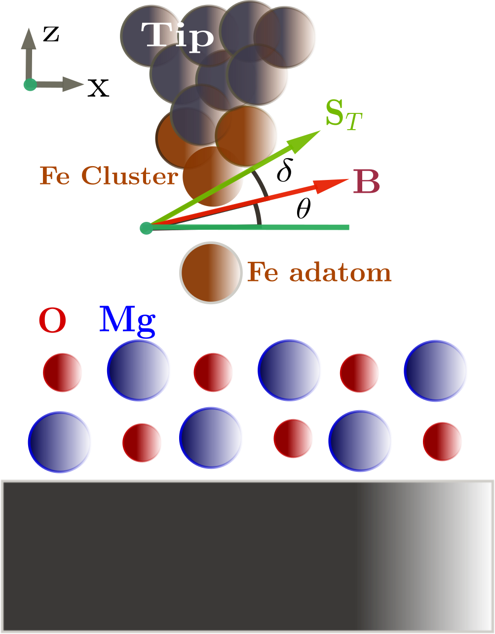
Figure 1: Sketch of a Fe atom in MgO/Ag and an SPSTM-tip

The rest of this paper is organized as follows. In sec. II, we present our models to address the problem of ESR-STM experiments in Fe at MgO. Sec. III is devoted to the study of the resonance frequency and the effect of the tip in ESR-STM experiments. We analyze, in detail, the possibility of optimizing the tip-sample interaction to perform ESR-STM experiments. In Sec. IV we propose a simple method to determine the main magnetic properties of the STM-tip. Finally in Sec. V we describe the most important findings and summarize the conclusions of the work.

II Model Hamiltonian

II.1 Spin Hamiltonian

The spin physics of individual adatoms can be described at two different levelsAbragam and Bleaney (1970). First, a multi-orbital electronic model for the outermost $d$ electrons, which includes Coulomb interactions, crystal field, and spin-orbit coupling, that we describe in Appendix A. The ground state manifold, obtained by numerical diagonalization, can be also described with an effective spin model. For the case of Fe on MgO the effective spin model, at zero field and ignoring coupling to the tip, is given byBaumann et al. (2015a, b); Ferrón et al. (2015, 2019):

$$\hat{H}_{eff}=-{\cal D}_{2}\hat{S}_{z}^{2}+{\cal D}_{4}\hat{S}_{z}^{4}-{\cal F}(\hat{S}_{+}^{4}+\hat{S}_{-}^{4})$$ (1)

where the spin operators act on the $S=2$ subspace. The anisotropy terms ${\cal D}_{2}$, ${\cal D}_{4}$ and ${\cal F}$ can be obtained from the diagonalization of the multi-orbital electronic model as shown in the Appendix B. Now, the spectrum of the ground state manifold has an EPR active space formed by a doublet of states with $S_{z}=\pm 2$. Yet, this doublet has a zero-field splitting (ZFS), given by $\Delta_{ZFS}=48{\cal F}=0.2$ $\mu$eV, due to quantum spin tunneling Klein (1952); Garg (1993); Delgado et al. (2015). We treat tip spin as a classical unit vector, $\vec{n}_{T}$. As a result, the interaction of the adatom with the tip can be treated as an effective field:

$${\cal H}_{1}=\mu_{B}\sum_{\beta=x,y,z}g^{\beta}B_{eff}^{\beta}S^{\beta}.$$ (2)

If the magnetic field is along the $z$ direction, we find that the gap between the ground state and the first excited state is

$$\Delta\approx 2\sqrt{(24{\cal F})^{2}+(2\mu_{B}g^{z}B_{eff}^{z})^{2}}\,.$$ (3)

This equation is still true if we add the component of the magnetic field along the $x$ direction, as long as the Zeeman energy associated to $B_{eff}^{x}$ is smaller than ${\cal D}_{2}+{\cal D}_{4}$, as we show in Appendix B. In the present case, the effective field $\vec{B}_{eff}$ is the sum of three contributions, external magnetic field, dipolar field of the tip, and exchange field of the tip:

$$B^{\beta}_{eff}=B^{\beta}+\frac{J_{ex}(z)}{g^{\beta}\mu_{B}}n_{T}^{\beta}+B^{\beta}_{dip}\equiv B^{\beta}+B^{\beta}_{\rm tip}$$ (4)

where $B^{\beta}$ is the $\beta=x,y,z$ component of the external magnetic field,

$$J_{ex}(z)=\langle S_{tip}\rangle J_{0}\,e^{-z/l_{0}}$$ (5)

is the distance-dependent tip-adatom exchange, $S_{tip}$ is the spin of the tip and $n_{T}^{\beta}$ are the components of the unit vector that describes the orientation of the tip spin. In the rest of the work, and so that our results show agreement with the experiments, we will use $J_{0}=20$ eV, $l_{0}=0.04$ nm and $\langle S_{tip}\rangle=2$.

Given the $C_{4}$ symmetry of the Fe adatom on top of an oxygen atom on the 001 MgO surface, we can assume the external field lies in the xz plane:

$$\vec{B}=B(\cos\theta,0,\sin\theta)$$ (6)

Because of its magnetic anisotropy, the tip magnetization can be misaligned from the external field by an angle $\delta$:

$$\vec{n}_{T}=(\cos(\theta+\delta),0,\sin(\theta+\delta))$$ (7)

The dipolar interaction between the magnetic moment of the tip and the surface spin comes from the magnetic field created by the tip,

$$\vec{B}_{dip}=\frac{\mu_{0}}{4\pi}\left(3\frac{(\vec{m}\cdot\vec{d})\vec{d}}{d^{5}}-\frac{\vec{m}}{d^{3}}\right)$$ (8)

where $\vec{m}=g_{\rm tip}\mu_{B}\langle S_{tip}\rangle\vec{n}_{T}\equiv M_{\rm tip}\vec{n}_{T}$. Of course, $M_{\rm tip}$ depends on the number of atoms in the tip. In the literatureWillke et al. (2019a) values of $M_{\rm tip}\simeq 10\mu_{B}-40\mu_{B}$ seems to be reasonable. In the rest of the work, and so that our results show agreement with some of the last experiments, we will use $M_{\rm tip}=30\mu_{B}$. When the Fe atom is just above the O atom we have $\vec{B}_{dip}=\,\mu_{0}\,M_{tip}\hat{n}_{dip}/(4\pi|z|^{3})$, where $\hat{n}_{dip}=(\cos(\theta+\delta),0,-2\,\sin(\theta+\delta))$.

Altogether, we arrive to the following expression for the $z$ component of the effective field acting on the Fe adatom:

$$B_{eff}^{(z)}=\left(\frac{J_{ex}(z)}{g^{z}\mu_{B}}-2\frac{\mu_{0}\,M_{tip}}{4\pi|z|^{3}}\right)\sin(\theta+\delta)+B\sin\theta$$ (9)

II.2 Effect of the tip-electric field on the surface spin

In actual EPR-STM experiments, there is a $DC$ bias, with amplitude $V_{DC}$, superimposed to the $AC$ bias $V_{RF}\sin{(\omega t)}$. Applying an electric field induces a strain $\delta z$ of the bond between the Fe adatom and the oxygen atom underneath Lado et al. (2017). This leads to a modulation of the crystal field Lado et al. (2017); Ferrón et al. (2019) and the magnetic field induced by the tipLado et al. (2017) (see Appendix C). The electric field across the gap between the STM and the MgO surface, $E=V_{DC}/d$, where $d$ is the tip-MgO distance, induces a force on the adatom, $F=qV_{DC}/d$ on account of its charge $q$. This force is compensated by a restoring elastic force $F=-k\delta z$. Then, we can evaluate how much the Fe atom is displaced from its equilibrium position Lado et al. (2017):

$$\delta z=\frac{qV_{DC}}{kd}$$ (10)

With this sign convention, increasing $V_{DC}$ leads to a stretching of the Fe-O bond and a reduction of the tip-Fe distance. In the present case we have $q=2$ and, from DFT calculations for Fe on MgO Lado et al. (2017); Ferrón et al. (2019), we obtain $k=600$ eV nm^-2. We find a modulation of the crystal field parameters in the multi-orbital fermionic model (see Appendix A and Appendix C) whose low energy states are described by Eq. (1). Using DFT calculations, we have computed this dependence for Fe on MgO Lado et al. (2017); Ferrón et al. (2019). Numerical diagonalization of the multi-orbital model that takes into account the modulation of the crystal field parameters as we described in Appendix C gives:

$${\cal D}_{i}={\cal D}_{i_{eq}}+\alpha_{{\cal D}_{i}}\,\delta z$$

$${\cal F}={\cal F}_{eq}+\alpha_{{\cal F}}\,\delta z$$

$$g^{\beta}=g^{\beta}_{eq}+\alpha_{g^{\beta}}\,\delta z$$ (11)

where the equilibrium parameters are those corresponding to a zero electric field when the piezoelectric displacement is not present. The parameters $\alpha_{X}$ are defined and evaluated in Appendix C and account for the effect of the piezoelectric displacement on the atom-surface interaction.

The combination of the piezoelectric distortion of the atom-tip distance due to the external electric field (Eq. (10)) and the crystal field parameter modulation (Eq. (II.2)) lead also to a modulation of the effective tip-induced field:

$$\frac{\partial B^{\beta}_{eff}}{\partial z}=\frac{\partial J_{ex}(z)}{\partial z}\frac{1}{g^{\beta}\mu_{B}}n^{\beta}+\frac{\partial B^{\beta}_{dip}}{\partial z}-\frac{J_{exc}(z)}{(g^{\beta})^{2}\mu_{B}}\,\frac{\partial g^{\beta}}{\partial z}$$ (12)

Finally, we can express the shift in the adatom resonance frequency, $f=\Delta/h$, as follows:

$$\delta f=\frac{\partial f}{\partial B^{\beta}_{eff}}\frac{\partial B^{\beta}_{eff}}{\partial z}\,\delta z+\frac{\partial f}{\partial{\cal F}}\frac{\partial{\cal F}}{\partial z}\,\delta z+\frac{\partial f}{\partial g^{\beta}}\frac{\partial g^{\beta}}{\partial z}\,\delta z$$ (13)

with $\beta=z$.

III Sweet spots for optimal tip-sample interactions

We now study how to optimize experimental parameters in the ESR-STM setup, such as the tip-adatom distance $d_{\rm tip}$ and the DC voltage $V_{DC}$. Specifically, we devote ourselves to describing two special points of operation. First, the optimal $d_{\rm tip}$ for which the effective magnetic field vanishes. The second, the regions in the $d_{\rm tip},V_{DC}$ plane where the variation of the frequency with respect to $V_{DC}$ is either large, affording voltage-controlled resonance frequency, or vanishing, which will mitigate dephasing.

III.1 No-tip influence distance

To establish to what extent the magnetic field induced by the tip affects the measurements, we must know how the resonance frequency, given in Eq. (3) behaves as a function of tip-sample distance when we experiment with different STM tips.

The influence of the tip arises from the $z$ component of the total magnetic field term (see Eq. (9)). It is important to note that ${\cal F}$ is small and therefore, in most situations, we can usually assume that $\Delta\simeq 4\mu_{B}g_{z}B_{eff}{(z)}$. In Fig. 2 we depict the ESR frequency as a function of the tip-adatom distance for different values of the tip anisotropy, $\delta$ (see Fig. 1). In solid lines, we show the corresponding calculations obtained by direct diagonalization of our multi-orbital electronic model (see Appendix A) for two different experimental situations. Filled dots in Fig. 2 show calculations performed using the perturbative expression Eq. (3). Panel (a) corresponds to an external magnetic field almost in-plane Willke et al. (2019a, 2018a, 2018b, b); Yang et al. (2018, 2017, 2019a) while in panel (b) an out-of-plane external magnetic field is applied Seifert et al. (2020b). Expectedly, the resonance frequency goes to a plateau-like regime for a large atom-tip distance, as both exchange and dipolar interactions fade away.

Interestingly, we observe in Fig. 2 a point at which all the curves intersect at a value approximately given by $4\mu_{B}g_{z}B_{z}$, independent of the dipolar and exchange field of the tip. This happens when the off-plane component of the tip field vanishes, ${B}_{tip}^{(z)}=0$ (see Eq. (4) and Eq. (9)). Using the expressions for the dipolar and exchange fields we obtain an implicit equation for the tip-atom distance $d_{n}$ for which these two contributions cancel each other:

$$J_{0}e^{-d_{n}/l_{0}}=\frac{g^{z}\gamma_{t}M_{tip}}{d_{n}^{3}},$$ (14)

where $\gamma_{t}=\mu_{B}\mu_{0}/4\pi$. For the choice of $J_{0}$, $l_{0}$ and $M_{tip}$, we find the NOTIN point at $d_{n}=0.59$ nm.

We observe, for the parameters employed in Fig. 2, that displacements of $10$ pm from the NOTIN point produce tip magnetic fields of $50$ mT. Although the NOTIN position seems to be optimal to carry out most of the measurements, it is clear that any small tip drift or tip vibration can make the scenario a little more complex by inducing unwanted magnetic fields and unexpected frequency alterations. For instance, the NOTIN distance has a small dependence on $V_{DC}$, by virtue of the piezoelectric displacement of the surface atom and the modulation of its $g$ factor, given in eq. (II.2). For the chosen value of tip parameters and up $V_{DC}=200mV$, we obtain changes around 2 pm in the NOTIN tip position.

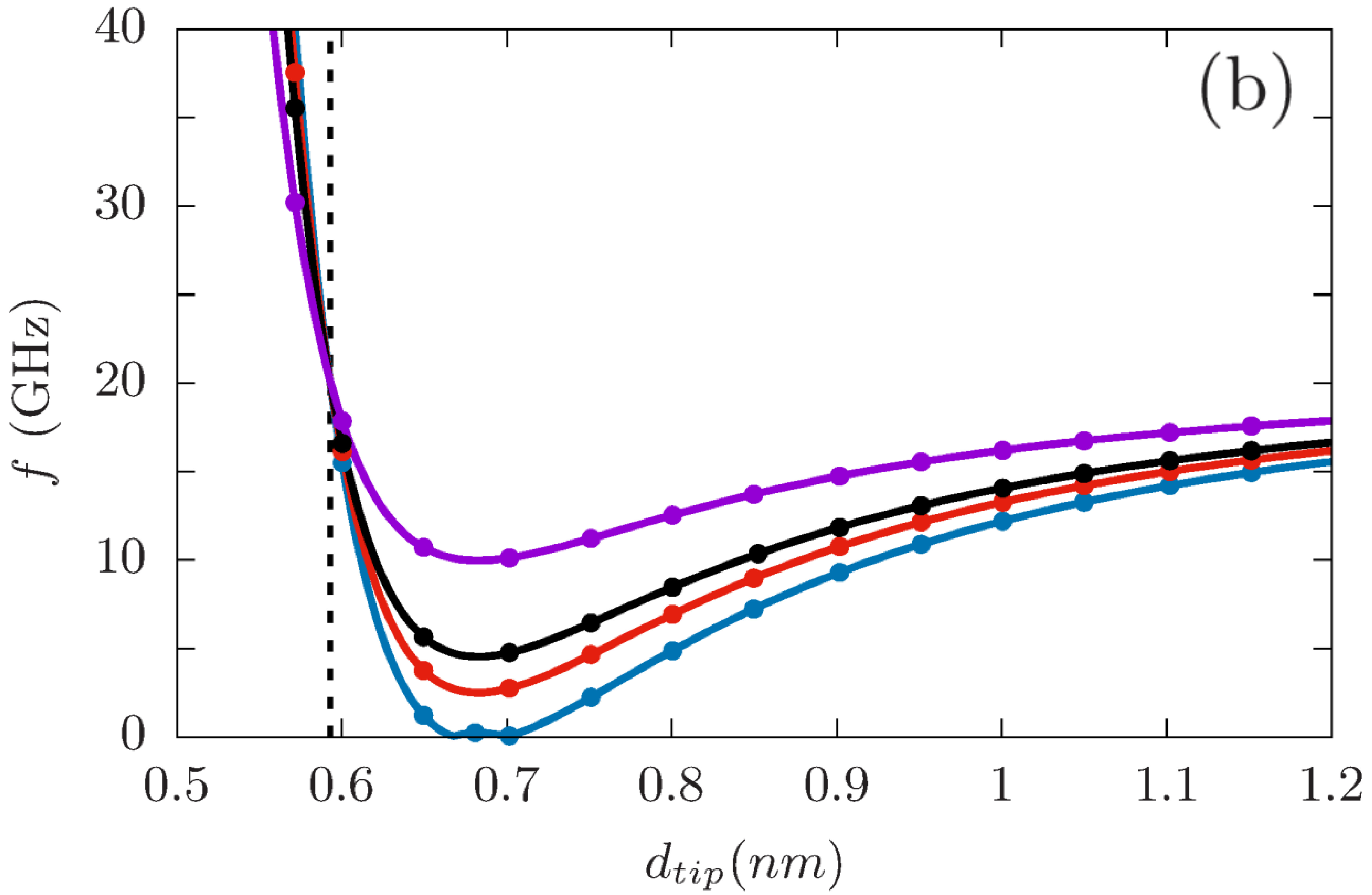
Figure 2: Resonance frequency as a function of the tip atom distance for different values of the tip anisotropy $\delta$. Panel (a) shows results for $\theta=8^{\circ}$ and $B_{ext}=0.9$ T. Panel (b) corresponds to the results with $\theta=90^{\circ}$ and $B_{ext}=0.1$ T. Solid lines show results obtained by direct diagonalization of the multi-orbital model while dots represent perturbative results obtained using Eq. (3).

III.2 Control of the $V_{DC}$ dependence

We now analyze how DC electric field of the tip changes the resonance frequency of the surface spin. This dependence arises from the combination of the piezoelectric displacement of the surface atom (Eq. 10) and the distance dependence of the frequency (Eq. 13). Depending on the target application, this dependence could be either a resource, for instance, to control $f$ without modifying the applied magnetic field, or a problem to avoid, as it can bring additional dephasing, as discussed below. In order to quantify these matters, we define the variation of the resonant frequency $f$ with respect to its $V_{DC}=0$ value,

$$\delta f=f(V_{DC})-f(V_{DC}=0)$$ (15)

The contour map of Fig. 3 (a) shows $|\delta f|$ (Eq. 15) as a function of both the external voltage and the tip-atom distance, for $\theta=8^{\circ}$, $\delta=60^{\circ}$ and $B_{ext}=0.9$ T. We focus our attention first on regions where $\delta f$ is small. This happens both for $d\simeq 0.7$nm and $d\simeq 0.9$ nm. In these two regions we have $df/dV_{DC}=0$ (see Eq. 3) at $V_{DC}=0$.

We now discuss how a small value of $df/dV_{DC}$ mitigates decoherence. It is known that, for a two-level system, stochastic fluctuations of fluctuating energy difference lead to pure dephasing. Specifically, let us write the effective field as the sum of the static contribution and a time-dependent fluctuation part, $B_{eff}^{z}=B_{eff,0}^{z}+b(t)$. For the fluctuation function, we assume that the time average vanishes, $\overline{b(t)}=0$ but has finite short memory fluctuations over time, ${\cal S}_{b}(t)\equiv\overline{b(t)b(t+\tau)}$ that decay rapidly when $t>>\tau$, and have an amplitude that scale with $b_{0}^{2}$. We define the Fourier transform $k(\omega)\equiv\frac{1}{2}\int_{-\infty}^{\infty}\overline{b(t)b(t+\tau)}e^{-i\omega t}dt$. We thus see that the stochastic field is characterized by the amplitude $b_{0}$ and a correlation time $\tau$. We can write down the decoherence rate asDelgado and Fernández-Rossier (2017):

$$\frac{1}{T_{2}}=\frac{(2g^{z}\mu_{B})^{2}}{\hbar}k(0)\propto\frac{(2g^{z}\mu_{B})^{2}}{\hbar}b_{0}^{2}\tau_{0}$$ (16)

We note this dephasing mechanism is independent of the current-induced dephasing that has been observed experimentallyWillke et al. (2018a), and would act even if no current is tunneling through the surface spin. Now, it is apparent both electrical noise in $V_{DC}$, $\delta V_{DC}(t)$, and mechanical noise in $\delta z(t)$ will contribute to the amplitude of the fluctuations of the effective field:

$$b(t)=\frac{\partial B_{eff}^{z}}{\partial z}\left(\frac{\partial z}{\partial V_{DC}}\delta V_{DC}(t)+\delta z(t)\right)$$ (17)

and thereby to dephasing. Therefore, having both a small $df/dV_{DC}$ and a small $df/dz$ will eliminate this source of decoherence. Importantly, since the ESR-STM driving of Fe on MgO is associated to the in-plane component of the effective fieldLado et al. (2017) and the frequency is dominated by the off-plane component, it is possible to have a vanishing $df/dz$, and at the same time a large Rabi coupling.

We now focus on the regions where $df/dV_{DC}$ is not small so that the DC bias could be used to achieve electrical control of the resonance frequency. In Fig. 3 (b) we plot the change as a function of applied external voltage for five particular tip-atom distances. For $d_{c1}\simeq 0.67$ nm (violet line) and $d_{c2}\simeq 0.9$ (cyan dashed line) we retrieve the stable regions discussed above, for which $f$ is independent of $V_{DC}$. In contrast, for the other three values of $d_{tip}$ we find a strong dependence of $f$ on $V_{DC}$. We draw attention to the immense value of $df/dV_{DC}$ at the NOTIN point.

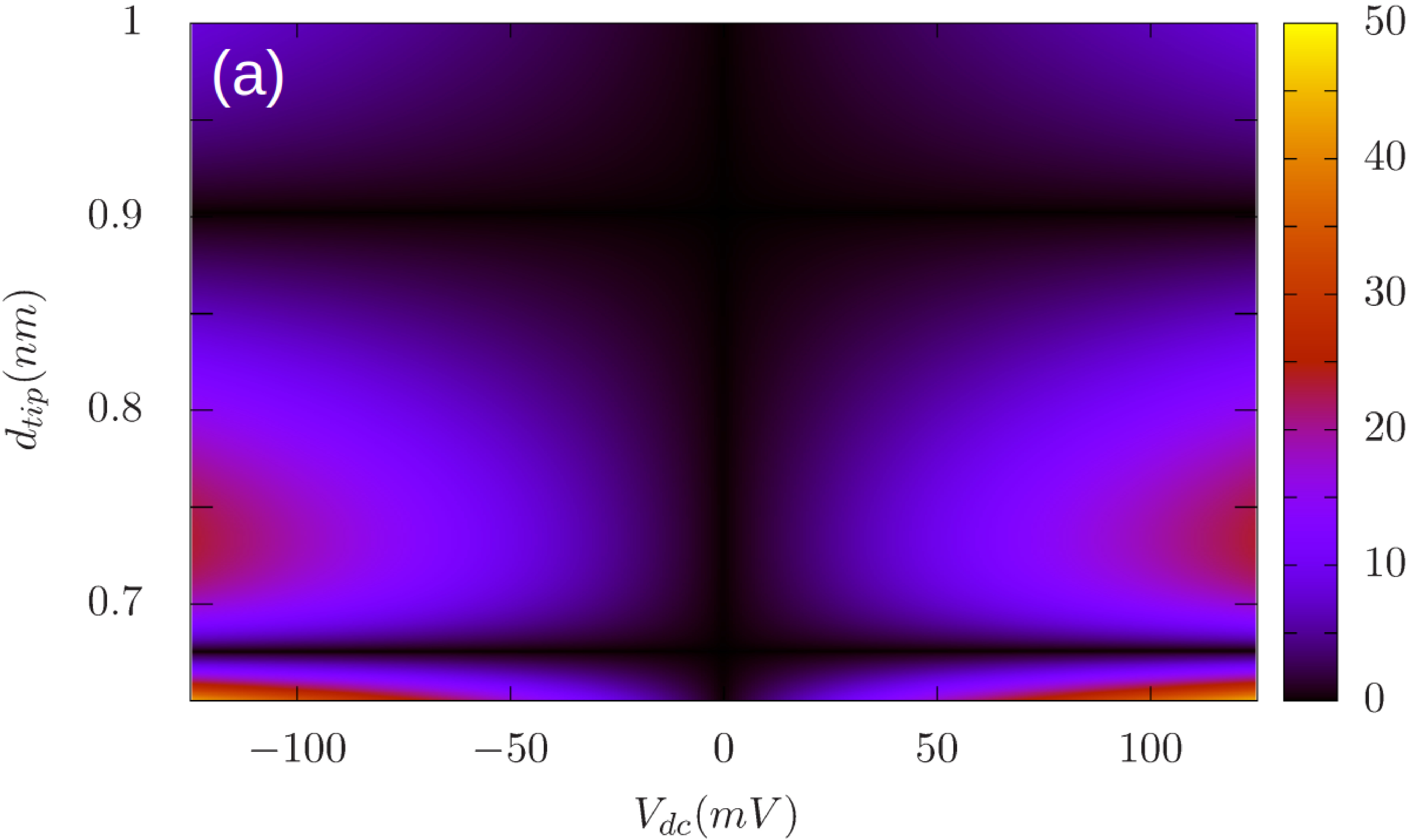
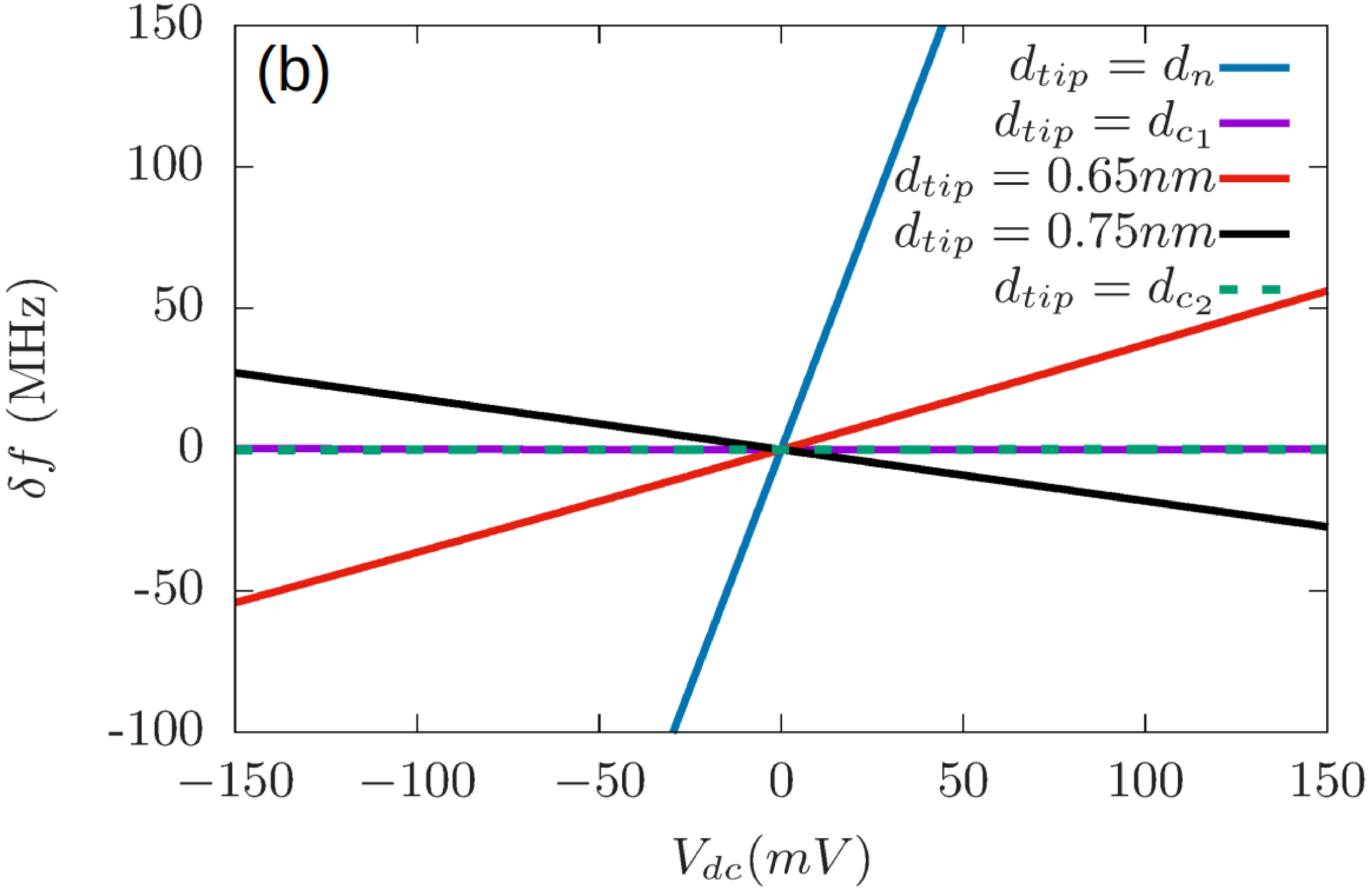
Figure 3: Shift of the resonance frequency versus $V_{DC}$ (Eq. (15) ). (a) Contour map of $|\delta f|$ as a function of the tip atom distance and external voltage for $\delta=60^{\circ}$ and $B=0.9$ T almost in-plane ($\theta=8^{\circ}$). In Panel (b) we plot the shift $\delta f$ (a horizontal section of the map) as a function of the external voltage for five different tip-atom distances.

IV Determination of tip anisotropy

So far, we have assumed that $\delta$, the misalignment angle between the tip magnetic moment and the external magnetic field, is unknown and can take values in a rather wide range, going from almost 0 ^∘ up to 60^∘ Yang et al. (2019a); Seifert et al. (2020b). The origin of this misalignment is necessarily related to some type of tip magnetic anisotropy that can arise both from anisotropy in the $g$ factor and single-ion anisotropies.

We now propose a simple experiment to determine $\delta$, similar to the one carried out by Kim et al. Kim et al. (2021) to probe the magnetic anisotropy of hydrogenated Ti on the surface of MgO. Essentially, we propose to measure the resonant frequency for Fe on MgO as a function of the angle $\theta$ formed between the external magnetic field and the surface, away from the NOTIN point. Our calculations (see Fig. 4) show a marked dependence of $f$ on $\theta$, expected because the Fe atom is sensitive mostly to the $z$ component of the effective field. We note how, for different values of $\delta$, our calculations show a lateral shift of the curves. Specifically, we find a dependence of the maximum as a function of the tip anisotropy $\delta$.

Imposing that the derivative of Eq. (3) with respect to $\theta$ vanishes and using Eq. (9), we obtain the following implicit equation for $\delta$

$$\tan(\theta_{max})=\frac{\varepsilon_{ext}+\varepsilon_{tip}\,\cos{(\delta)}}{\varepsilon_{tip}\,\sin{(\delta)}}\,.$$ (18)

where

$$\varepsilon_{ext} = \,g^{z}\mu_{B}\,B\,,$$

$$\varepsilon_{tip} = \varepsilon_{exc}-\varepsilon_{dip}\,,$$

$$\varepsilon_{exc} = 2J_{0}\,e^{-z/l_{0}}\,,$$

$$\varepsilon_{dip} = 2\gamma_{t}\frac{g^{z}\,M_{tip}}{|z|^{3}}\,,$$ (19)

$g_{z}$ is defined in Eq. (II.2) and $z=d_{\rm tip}-\delta z$. Thus, experimental determination of $\theta_{max}$ and the tip effective fields, $\varepsilon_{tip}$ and $\varepsilon_{exc}$, permit to read out the value of $\delta$. Importantly, in the limit of a very small magnetic field, we have a simple linear relation between $\delta$ and $\theta_{max}$, independent of $\varepsilon_{tip}$ and $\varepsilon_{exc}$,

$$\delta=\frac{\pi}{2}-\theta_{max}.$$ (20)

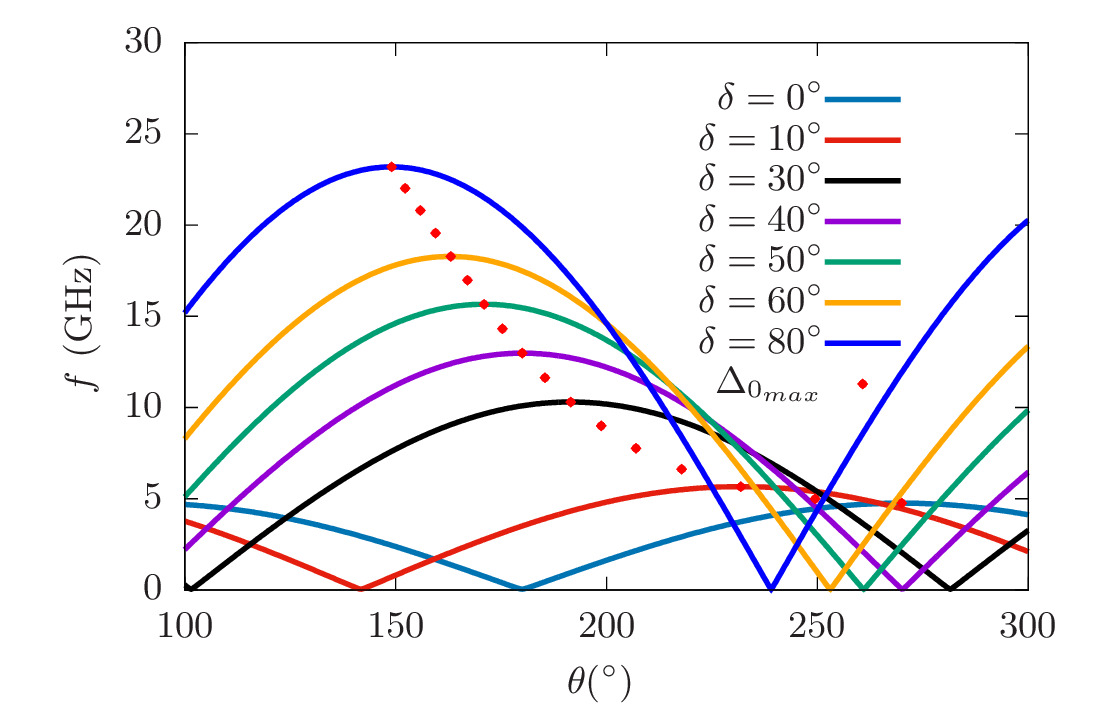
Figure 4: Resonance frequency as a function of the external magnetic orientation, $\theta$, for different values of $\delta$. The calculation was performed by exact diagonalization of the few electron model (see appendix A). All the calculations were performed for $B=0.1$ T, $d_{tip}=0.7$ nm and a strong dipolar contribution $M_{tip}=30\,\mu_{B}$.

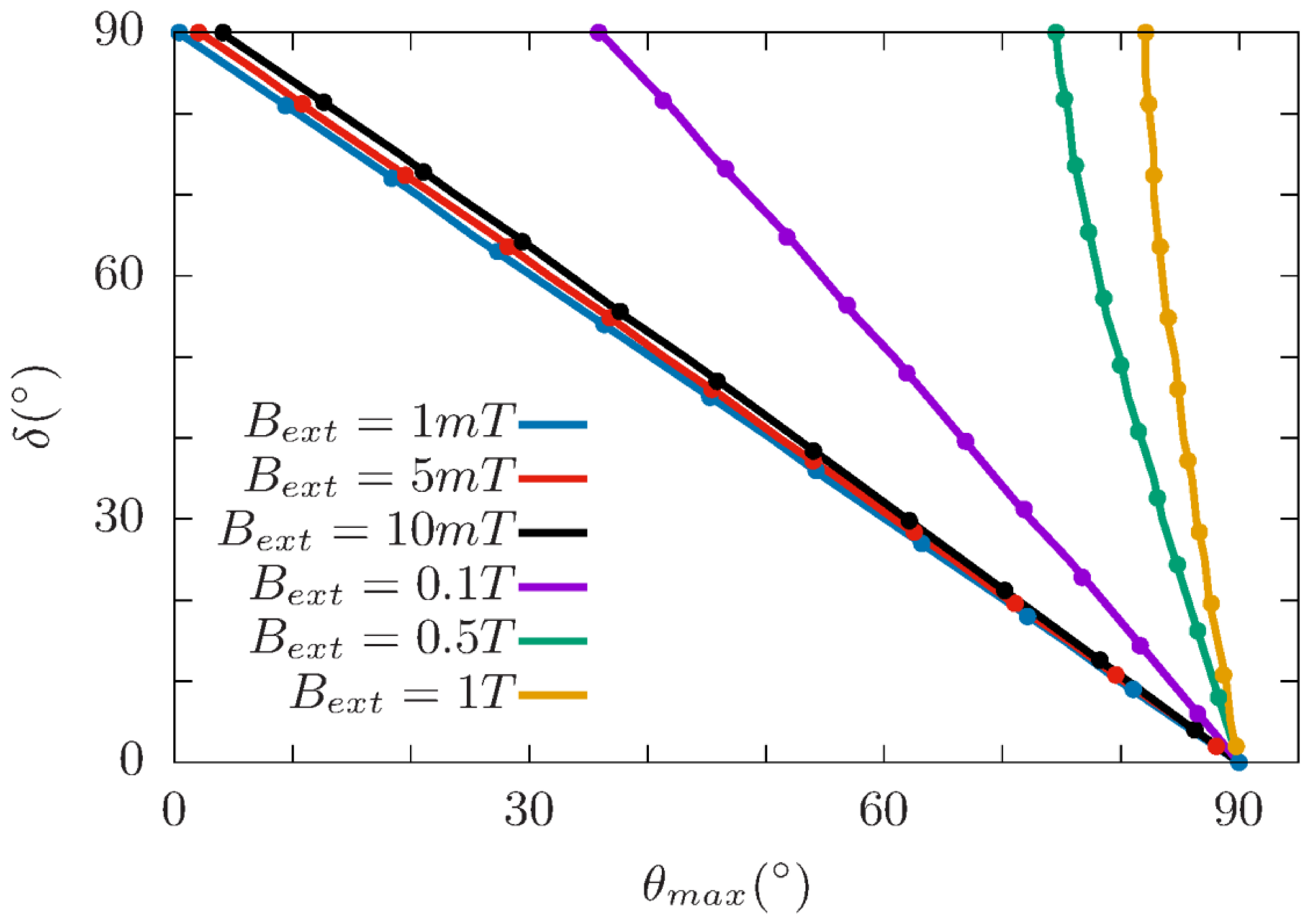
Figure 5: Detuning angle $\delta$ (see Eq. (7)) as a function of $\theta_{max}$ (see Fig. 4) obtained with two methods: solid lines show the results obtained from the exact diagonalization of the few electron model while dots show results obtained from the transcendental Eq. (18).

In Fig. 5 we plot the anisotropy angle $\delta$ as a function of $\theta_{max}$ for different values of the external magnetic field. Solid lines and filled circles show an excellent agreement of the results obtained by numerical diagonalization of our multi-orbital model and the ones obtained from solving Eq. (18). It is clear from this figure that in the small magnetic field limit ($B_{ext}\rightarrow 0$) all the curves converge to the expression in Eq. (20). This suggests that carrying out the experiments with small magnetic fields (it is even possible to carry them out at a vanishing field Willke et al. (2019b)) would make it possible to estimate the misalignment angle $\delta$ without having to infer the values of $\varepsilon_{dip}$ and $\varepsilon_{exc}$. We also note that, in this limit, the relation between $\delta$ and $\theta_{max}$ is independent of $V_{DC}$, which should simplify the experiment.

V Summary and conclusions

In this work we have studied the interactions between a STM tip and a single Fe atom on an MgO surface, relevant for single spin ESR-STM experimentsBaumann et al. (2015a); Willke et al. (2018a). The tip influences the surface spin via three different mechanisms: dipolar coupling, exchange interactions, and the electric coupling that induces piezoelectric displacements of the Fe ion, modulating both its spin interactions with the tip as well as its $g$ factor and crystal field parameters. All these interactions produce shifts of the Fe energy levels and a modification of the resonance frequency $f$. Therefore, in order to use the surface spin as a sensor for magnetometry, it is important to assess the tip contributions.

We have discussed first the existence of a sweet spot at which the dipolar and exchange spin couplings cancel each other, the so called NOTIN point. In figure 2 we have calculated the NOTIN point for $V_{DC}=0$. We have then discussed the influence of $V_{DC}$ on the resonance frequency $f$. We have calculated a phase diagram for the stability of $f$ with respect to variations in $V_{DC}$ as a function of both tip-atom distance $d_{tip}$ and $V_{DC}$. We stress that two different regimes may be of practical interest. First, the regions in this phase diagram where the frequency is very stable with respect to voltage fluctuations. We have discussed how in this region decoherence due to both mechanical and electrical noise would be mitigated. Second, regions in which large variations of the resonant frequency can be obtained by changing $V_{DC}$. Whereas this would increase decoherence it would permit an electrical control of the resonant frequency that may be convenient in some situations.

All of our results depend on $\delta$, the misalignment angle between the tip magnetization and the external magnetic field. We propose the following experimental protocol to measure $\delta$, based on measuring $f(\theta)$, where $\theta$ is the orientation of the applied field. We find that the maxima of this curve depend on $\delta$ and in the limit of vanishing external field, this relation is straightforward: these angles, $\theta$ and $\delta$, are dephased by $90^{\circ}$ (see Eq. (20)).

These results may help the design of future ESR-STM experiments, especially in cases where accurate magnetometry is required del Castillo and Fernández-Rossier (2022); Karjalainen et al. (2022). In this work, we have focused on the case of Fe adatoms on MgO. Similar results should be obtained in the case of other ESR-STM active adatoms, such as Ti-H on MgO, with quantitative modification arising from the differences of $g$ factor anisotropies and magnetic moments between these systems.

Appendix A Multi-orbital Electronic Model

We start with the Hamiltonian for the 6 electrons in the $d$-levels of Fe:

$${\cal H}_{\rm Fe}=H_{\rm CF}+H_{\rm SO}+H_{\rm Z}+H_{ee}+H_{\rm Tip}$$ (21)

where $H_{\rm CF}$ is the crystal field Hamiltonian, $H_{\rm SO}$ is the spin-orbit coupling, $H_{\rm Z}$ is the Zeeman Hamiltonian, $H_{ee}$ is the Coulomb term and $H_{\rm Tip}$ accounts for the interaction of the atom with the tip. The Crystal Field part of the Hamiltonian is obtained from the representation of the DFT Hamiltonian in the basis of maximally localized Wannier orbitals Marzari et al. (2012); Ferrón et al. (2015, 2015); Lado et al. (2017)

$$H_{CF}=\frac{1}{2}\sum_{m,m^{\prime},\sigma}\langle m|h_{\rm CF}|m^{\prime}\rangle d_{m\sigma}^{\dagger}d_{m^{\prime}\sigma},$$ (22)

where $d_{m\sigma}^{\dagger}$ ($d_{m\sigma}$) denotes the creation (annihilation) operator of an electron with spin $\sigma$ in the $\ell=2,\ell_{z}=m$ state of the Fe atom, denoted by $\phi_{m}(\vec{r})$, assumed to be equal to the product of a radial hydrogenic function (with effective charge $Z$ and a effective Bohr radius $a_{\mu}$) and a spherical harmonic. The one-particle elements are calculated from Lado et al. (2017)

$$h_{\rm CF}=Dl_{z}^{2}+F\left(l_{x}^{4}+l_{y}^{4}\right)$$ (23)

where $D=-290$ meV, and $F=-10$ meV are Crystal Field parameters obtained from DFT calculations and Wannierization Lado et al. (2017); Ferrón et al. (2019). We add the spin-orbit coupling operatorFerrón et al. (2015, 2015); Lado et al. (2017)

$$H_{\rm SO}=\lambda_{SO}\,\sum_{mm^{\prime},\sigma\sigma^{\prime}}\langle m\sigma|\vec{\ell}\cdot\vec{S}|m^{\prime}\sigma^{\prime}\rangle d_{m\sigma}^{\dagger}d_{m^{\prime}\sigma^{\prime}},$$ (24)

where we take $\lambda_{SO}=35$ meV Lado et al. (2017); Ferrón et al. (2015). Zeeman Hamiltonian reads:

$$H_{\rm Z}=\mu_{B}\vec{B}\cdot\sum_{mm^{\prime},\sigma\sigma^{\prime}}\langle m,\sigma|\left(\vec{l}+g\vec{S}\right)|m^{\prime}\sigma^{\prime}\rangle d_{m\sigma}^{\dagger}d_{m^{\prime}\sigma^{\prime}},$$ (25)

where $g=2$. The Coulomb term reads:

$$H_{{\rm ee}}=\frac{1}{2}\sum_{m,m^{\prime}\atop n,n^{\prime}}V_{mnm^{\prime}n^{\prime}}\sum_{\sigma\sigma^{\prime}}d_{m\sigma}^{\dagger}d_{n\sigma^{\prime}}^{\dagger}d_{n^{\prime}\sigma^{\prime}}d_{m^{\prime}\sigma},$$ (26)

For the evaluation of the Coulomb integrals $V_{mnm^{\prime}n^{\prime}}$ we transform the angular part to a basis of eigenstates of $l=2$. In the basis of eigenstates of $l=2$, all the Coulomb integrals scale linearly with the value of $V_{0000}=U$Ferrón et al. (2015, 2015). Here we take, as in previous works, $U=5.0$ eV Lado et al. (2017); Ferrón et al. (2015). Now, to end with an adequate description of the situation, we need to describe the interaction of the atom with the tip. Along this work, we consider exchange and dipolar interaction $H_{Tip}=H_{\rm ex}+H_{\rm dip}$. We can write the exchange interaction as $J_{ex}(z)\vec{S}_{tip}\cdot\vec{S}$ Lado et al. (2017) where $S_{tip}$ is the total spin of the spin-polarized tip and $J_{ex}$ is the exchange coupling between the surface spin and the tip. The exchange coupling depends exponentially on the tip-adatom distance and it can be written Lado et al. (2017):

$$J_{ex}(z)=J_{0}\,e^{-z/l_{0}}\,.$$ (27)

where $J_{0}$ and $l_{0}$ depend on the tip and the adatom. The exchange coupling can be written as in most of the experimental worksWillke et al. (2019a) as $J_{ex}(z)=J^{\ast}_{0}\,e^{-(z-z_{pc})/l_{0}}$ by doing $J_{0}=J^{\ast}_{0}e^{z_{pc}/l_{0}}$ and $z_{pc}$ is the tip heights above point contact and can be measured for Ti ($z_{pc}\simeq 0.3$ nm) and Fe ($z_{pc}\simeq 0.4$ nm) atoms Willke et al. (2019a). We ignore the quantum fluctuations of the magnetic moment of the apex atom or atoms, quenched by the combination of an applied magnetic field and strong Korringa damping with the tip electron bathDelgado et al. (2014). Therefore, we treat the tip spin in a mean-field or classical approximation, following [Yan et al., 2015; Lado et al., 2017], and replace $S_{tip}$ by its statistical average $\langle S_{tip}\rangle$. Then, the tip-atom exchange interaction contribution to the Hamiltonian reads

$$H_{\rm ex}=J_{ex}\langle\vec{S}_{tip}\rangle\cdot\sum_{mm^{\prime},\sigma\sigma^{\prime}}\langle m,\sigma|\vec{S}|m^{\prime}\sigma^{\prime}\rangle d_{m\sigma}^{\dagger}d_{m^{\prime}\sigma^{\prime}},$$ (28)

where $\braket{\vec{S_{tip}}}=\braket{S_{tip}}\hat{n}_{T}$ and $\hat{n}_{T}=(\cos(\theta+\delta),0,\sin(\theta+\delta))$ (see Fig. 1).

The dipolar interaction between the magnetic moment of the tip and the surface spin, where the tip creates a magnetic field whose orientation depends on the tip characteristics, gives us a dipolar term of the form:

$$H_{\rm dip}=\mu_{b}\vec{B}_{dip}\cdot\sum_{mm^{\prime},\sigma\sigma^{\prime}}\langle m,\sigma|\left(\vec{l}+g\vec{S}\right)|m^{\prime}\sigma^{\prime}\rangle d_{m\sigma}^{\dagger}d_{m^{\prime}\sigma^{\prime}},$$ (29)

where the effective magnetic field created by the tip is defined in Eq. (8).

The few-body Hamiltonian 21 is solved exactly, by numerical diagonalization in a space constructed with all the states that accommodate six electrons in five spin-degenerate $d$ orbitals.

Appendix B Effective spin model

The lowest energy manifold of the Hamiltonian defined in the previous section has five states separated from the rest of the spectra. These states correspond to a ground state with $S=2$ result of accommodating 6 electrons in 5 $d$ orbitals and can be described in terms of a simple effective spin model Ferrón et al. (2015, 2019):

$$\hat{H}_{eff}=-{\cal D}_{2}\hat{S}_{z}^{2}+{\cal D}_{4}\hat{S}_{z}^{4}-{\cal F}(\hat{S}_{+}^{4}+\hat{S}_{-}^{4})+{\cal H}_{1}\,.$$ (30)

where the spin operators act on the $S=2$ subspace. The term ${\cal H}_{1}$ accounts for the interaction of the adatom with the tip and the external field (see Eq. (4) and Eq. (2)). The anisotropy terms ${\cal D}_{2}$, ${\cal D}_{4}$ and ${\cal F}$ can be obtained from the diagonalization of Hamiltonian Eq. (21) with no magnetic field and no tip. We obtain ${\cal D}_{2}=4.86$ meV, ${\cal D}_{4}=0.23$ meV, and ${\cal F}=4.06$ neV. Now, the spectrum of the ground state manifold has an EPR active space formed by a doublet of states with $S_{z}=\pm 2$. Yet, this doublet has a zero-field splitting (ZFS), given by $\Delta=48{\cal F}=0.2$ $\mu$eV, due to quantum spin tunneling Klein (1952); Garg (1993); Delgado et al. (2015).

Our model for the Fe atom at MgO taking into account the interaction of the surface spin with the magnetic moment of the tip, described by Hamiltonian (21), can be solved by numerical diagonalization. We can calculate the resonance frequency $f=\Delta/h=(E_{1}-E_{0})/h$ as a function of the tip-atom distance $z=d_{tip}$ for different values of $J_{0}$ and $M_{tip}$. Comparing with experimentally determined parameters and the resonance frequency curves obtained experimentally Willke et al. (2018a, b, 2019b, 2019a); Seifert et al. (2020a); Seifert et al. (2021); Seifert et al. (2020b), in particular paying attention to the results presented in [Willke et al., 2019a], [Seifert et al., 2020b] and [Seifert et al., 2021], a reasonable set of values are $l_{0}=0.04-0.06$ nm, $J_{0}=10-60$ eV ($J^{\ast}_{0}=0.5-3$ meV) and $M_{tip}=10\mu_{B}-40\mu_{B}$.

Perturbative expresions

The eigenvalues of the effective spin Hamiltonian assuming $B_{eff}^{(x)}=0$ can be written

$$E_{4}=0\,,$$

$$E_{3}=-{\cal D}_{2}+{\cal D}_{4}+B_{eff}^{z}\,,$$

$$E_{2}=-{\cal D}_{2}+{\cal D}_{4}-B_{eff}^{z}\,,$$

$$E_{1}=-4{\cal D}_{2}+16{\cal D}_{4}+\sqrt{(24{\cal F})^{2}+(2B_{eff}^{z})^{2}}\,,$$

$$E_{0}=-4{\cal D}_{2}+16{\cal D}_{4}-\sqrt{(24{\cal F})^{2}+(2B_{eff}^{z})^{2}}\,,$$

and the eigenvectors

$$\ket{4}=\ket{S_{z}=0}\,,$$

$$\ket{3}=\ket{S_{z}=1}\,,$$

$$\ket{2}=\ket{S_{z}=-1}\,,$$

$$\ket{1}=C_{1}^{1}\ket{S_{z}=2}+C_{2}^{1}\ket{S_{z}=-2}\,,$$

$$\ket{0}=C_{1}^{0}\ket{S_{z}=2}+C_{2}^{0}\ket{S_{z}=-2}\,,$$

where $\{\ket{S_{z}=i}\}$ are eigenstates of $S_{z}$ for $S=2$. We introduce $B_{eff}^{x}$ as a perturbation. Using perturbation up to second order in $B_{eff}^{x}$, we have that

$$E_{i}^{(2)}=E_{i}^{(0)}+{\left(\mu_{B}g^{x}B_{eff}^{x}\right)}^{2}\,\sum_{m\neq i}^{4}\,\frac{|\braket{m}{\hat{S}_{x}}{i}|^{2}}{E_{i}^{(0)}-E_{m}^{(0)}}\,.$$ (31)

Assuming $B_{eff}<<{\cal D}_{i}$ with $i=2,4$ we obtain

$$E_{i}^{(2)}=E_{i}^{(0)}+\frac{3}{2}\,\frac{{\left(\mu_{B}g^{x}B_{eff}^{x}\right)}^{2}\,}{E_{i}^{(0)}-E_{3}^{(0)}}\,.$$ (32)

We thus see that, in the subspace of the two lowest energy states of the Fe adatom, the effect of $B_{x}$ is negligible, to linear order in $B_{x}$. and finally we can write the gap of the system as follows

$$\Delta\approx 2\sqrt{(24{\cal F)}^{2}+(2\mu_{B}g^{z}B_{eff}^{z})^{2})}$$ (33)

As the anisotropy terms, we obtain the $g$ tensor from the diagonalization of Hamiltonian Eq. (21). For the values quoted above and ignoring the effect of the tip, we get $g_{z}=2.8$.

Appendix C Effect of the external electric field on the Hamiltonian parameters

Our model assume a piezoelectric distortion of the atom-tip distance due to the external electric field. This distortion modulates crystal field parameters in the Hamiltonian Eq. (21):

$$F=F_{eq}+\frac{dF}{dz}\bigg{|}_{z_{eq}}\delta z\,,$$ (34)

$$D=D_{eq}+\frac{dD}{dz}\bigg{|}_{z_{eq}}\delta z\,,$$

and tip terms directly by their dependency with $\delta z$ through $z=d_{tip}-\delta z$ where $d_{tip}$ is the tip-atom distance at the equilibrium. Here we take, using DFT calculationsLado et al. (2017), $\frac{dF}{dz}\bigg{|}_{z_{eq}}=280\frac{meV}{nm}$ and $\frac{dD}{dz}\bigg{|}_{z_{eq}}=0$.

For the effective spin Hamiltonian Eq. (30) and Eq. (1) we can calculate the modulation of the parameters by direct diagonalization of Eq. (21) taking into account the modulation of the crystal field parameters described above:

$${\cal D}_{2}={\cal D}_{2_{eq}}+\alpha_{{\cal D}_{2}}\,\delta z$$

$${\cal D}_{4}={\cal D}_{4_{eq}}+\alpha_{{\cal D}_{4}}\,\delta z$$

$${\cal F}={\cal F}_{eq}+\alpha_{{\cal F}}\,\delta z$$

$$g^{x}=g^{x}_{eq}+\alpha_{g^{x}}\,\delta z$$

$$g^{z}=g^{z}_{eq}+\alpha_{g^{z}}\,\delta z\,.$$ (35)

with

$$\alpha_{X}=\frac{\partial X}{\partial F}\,\frac{\partial F}{\partial z}\bigg{|}_{z_{eq}}+\frac{\partial X}{\partial D}\,\frac{\partial D}{\partial z}\bigg{|}_{z_{eq}}.$$ (36)

Finally, calculated modulation and equilibrium parameters for the effective Hamiltonian are depicted in Table 1.

$X$	$X_{eq}$	$\alpha_{X}$
${\cal D}_{2}$	$4.9$ meV	$134$ $\mu$eV/pm
${\cal D}_{4}$	$0.2$ meV	$14$ $\mu$eV/pm
${\cal F}$	$4.1$ neV	$-0.0002$ $\mu$eV/pm
$g^{x}$	$2.0$	$-0.36$ nm-1
$g^{z}$	$2.8$	$-9.02$ nm-1

Table 1: Parameters of the effective Hamiltonian and their modulations.

References

- Manassen et al. (1989) Y. Manassen, R. Hamers, J. Demuth, and A. Castellano Jr, Physical Review Letters 62, 2531 (1989).
- Balatsky et al. (2012) A. V. Balatsky, M. Nishijima, and Y. Manassen, Advances in Physics 61, 117 (2012).
- Baumann et al. (2015a) S. Baumann, W. Paul, T. Choi, C. P. Lutz, A. Ardavan, and A. J. Heinrich, Science 350, 417 (2015a).
- Natterer et al. (2017) F. D. Natterer, K. Yang, W. Paul, P. Willke, T. Choi, T. Greber, A. J. Heinrich, and C. P. Lutz, Nature 543, 226 (2017).
- Choi et al. (2017) T. Choi, W. Paul, S. Rolf-Pissarczyk, A. J. Macdonald, F. D. Natterer, K. Yang, P. Willke, C. P. Lutz, and A. J. Heinrich, Nature nanotechnology 12, 420 (2017).
- Yang et al. (2017) K. Yang, Y. Bae, W. Paul, F. D. Natterer, P. Willke, J. L. Lado, A. Ferrón, T. Choi, J. Fernández-Rossier, A. J. Heinrich, et al., Physical review letters 119, 227206 (2017).
- Willke et al. (2018a) P. Willke, W. Paul, F. D. Natterer, K. Yang, Y. Bae, T. Choi, J. Fernández-Rossier, A. J. Heinrich, and C. P. Lutz, Science advances 4, eaaq1543 (2018a).
- Willke et al. (2018b) P. Willke, Y. Bae, K. Yang, J. L. Lado, A. Ferrón, T. Choi, A. Ardavan, J. Fernández-Rossier, A. J. Heinrich, and C. P. Lutz, Science 362, 336 (2018b).
- Bae et al. (2018) Y. Bae, K. Yang, P. Willke, T. Choi, A. J. Heinrich, and C. P. Lutz, Science advances 4, eaau4159 (2018).
- Yang et al. (2018) K. Yang, P. Willke, Y. Bae, A. Ferrón, J. L. Lado, A. Ardavan, J. Fernández-Rossier, A. J. Heinrich, and C. P. Lutz, Nature nanotechnology 13, 1120 (2018).
- Yang et al. (2019a) K. Yang, W. Paul, F. D. Natterer, J. L. Lado, Y. Bae, P. Willke, T. Choi, A. Ferrón, J. Fernández-Rossier, A. J. Heinrich, et al., Physical Review Letters 122, 227203 (2019a).
- Willke et al. (2019a) P. Willke, K. Yang, Y. Bae, A. J. Heinrich, and C. P. Lutz, Nature Physics 15, 1005 (2019a).
- Willke et al. (2019b) P. Willke, A. Singha, X. Zhang, T. Esat, C. P. Lutz, A. J. Heinrich, and T. Choi, Nano Letters 19, 8201 (2019b).
- van Weerdenburg et al. (2021) W. M. van Weerdenburg, M. Steinbrecher, N. P. van Mullekom, J. W. Gerritsen, H. von Allwörden, F. D. Natterer, and A. A. Khajetoorians, Review of Scientific Instruments 92, 033906 (2021).
- Steinbrecher et al. (2021) M. Steinbrecher, W. M. Van Weerdenburg, E. F. Walraven, N. P. Van Mullekom, J. W. Gerritsen, F. D. Natterer, D. I. Badrtdinov, A. N. Rudenko, V. V. Mazurenko, M. I. Katsnelson, et al., Physical Review B 103, 155405 (2021).
- Natterer et al. (2019) F. D. Natterer, F. Patthey, T. Bilgeri, P. R. Forrester, N. Weiss, and H. Brune, Review of Scientific Instruments 90, 013706 (2019).
- Hwang et al. (2022) J. Hwang, D. Krylov, R. Elbertse, S. Yoon, T. Ahn, J. Oh, L. Fang, W.-j. Jang, F. H. Cho, A. J. Heinrich, et al., Review of Scientific Instruments 93, 093703 (2022).
- Seifert et al. (2020a) T. S. Seifert, S. Kovarik, C. Nistor, L. Persichetti, S. Stepanow, and P. Gambardella, Physical Review Research 2, 013032 (2020a).
- Kot et al. (2022) P. Kot, M. Ismail, R. Drost, J. Siebrecht, H. Huang, and C. R. Ast, arXiv preprint arXiv:2209.10969 (2022).
- Veldman et al. (2021) L. M. Veldman, L. Farinacci, R. Rejali, R. Broekhoven, J. Gobeil, D. Coffey, M. Ternes, and A. F. Otte, Science 372, 964 (2021).
- Yang et al. (2021) K. Yang, S.-H. Phark, Y. Bae, T. Esat, P. Willke, A. Ardavan, A. J. Heinrich, and C. P. Lutz, Nature communications 12, 1 (2021).
- Kovarik et al. (2022) S. Kovarik, R. Robles, R. Schlitz, T. S. Seifert, N. Lorente, P. Gambardella, and S. Stepanow, Nano Letters (2022).
- Willke et al. (2021) P. Willke, T. Bilgeri, X. Zhang, Y. Wang, C. Wolf, H. Aubin, A. Heinrich, and T. Choi, ACS nano 15, 17959 (2021).
- Zhang et al. (2022) X. Zhang, C. Wolf, Y. Wang, H. Aubin, T. Bilgeri, P. Willke, A. J. Heinrich, and T. Choi, Nature Chemistry 14, 59 (2022).
- Farinacci et al. (2022) L. Farinacci, L. M. Veldman, P. Willke, and S. Otte, Nano Letters 22, 8470 (2022).
- Yang et al. (2019b) K. Yang, W. Paul, S.-H. Phark, P. Willke, Y. Bae, T. Choi, T. Esat, A. Ardavan, A. J. Heinrich, and C. P. Lutz, Science 366, 509 (2019b).
- Caso et al. (2014) A. Caso, B. Horovitz, and L. Arrachea, Physical Review B 89, 075412 (2014).
- Berggren and Fransson (2016) P. Berggren and J. Fransson, Scientific reports 6, 25584 (2016).
- Lado et al. (2017) J. L. Lado, A. Ferrón, and J. Fernández-Rossier, Physical Review B 96, 205420 (2017).
- Shakirov et al. (2019) A. M. Shakirov, A. N. Rubtsov, and P. Ribeiro, Physical Review B 99, 054434 (2019).
- Gálvez et al. (2019) J. R. Gálvez, C. Wolf, F. Delgado, and N. Lorente, Physical Review B 100, 035411 (2019).
- Ferrón et al. (2019) A. Ferrón, S. A. Rodríguez, S. S. Gómez, J. L. Lado, and J. Fernández-Rossier, Physical Review Research 1, 033185 (2019).
- Delgado and Lorente (2021) F. Delgado and N. Lorente, Progress in Surface Science 96, 100625 (2021).
- Seifert et al. (2021) T. S. Seifert, S. Kovarik, P. Gambardella, and S. Stepanow, Physical Review Research 3, 043185 (2021).
- Seifert et al. (2020b) T. S. Seifert, S. Kovarik, D. M. Juraschek, N. A. Spaldin, P. Gambardella, and S. Stepanow, Science advances 6, eabc5511 (2020b).
- Abragam and Bleaney (1970) A. Abragam and B. Bleaney, Electron Paramagnetic Resonance of Transition Ions (Oxford University Press, Oxford, 1970).
- Baumann et al. (2015b) S. Baumann, F. Donati, S. Stepanow, S. Rusponi, W. Paul, S. Gangopadhyay, I. Rau, G. Pacchioni, L. Gragnaniello, M. Pivetta, et al., Physical review letters 115, 237202 (2015b).
- Ferrón et al. (2015) A. Ferrón, J. L. Lado, and J. Fernández-Rossier, Phys. Rev. B 92, 174407 (2015).
- Klein (1952) M. J. Klein, Am. J. Phys. 20, 65 (1952).
- Garg (1993) A. Garg, EPL (Europhysics Letters) 22, 205 (1993).
- Delgado et al. (2015) F. Delgado, S. Loth, M. Zielinski, and J. Fernández-Rossier, EPL (Europhysics Letters) 109, 57001 (2015).
- Delgado and Fernández-Rossier (2017) F. Delgado and J. Fernández-Rossier, Progress in Surface Science 92, 40 (2017).
- Kim et al. (2021) J. Kim, W.-j. Jang, T. H. Bui, D.-J. Choi, C. Wolf, F. Delgado, Y. Chen, D. Krylov, S. Lee, S. Yoon, et al., Physical Review B 104, 174408 (2021).
- del Castillo and Fernández-Rossier (2022) Y. del Castillo and J. Fernández-Rossier, arXiv preprint arXiv:2211.14205 (2022).
- Karjalainen et al. (2022) N. Karjalainen, Z. Lippo, G. Chen, R. Koch, A. O. Fumega, and J. L. Lado, arXiv preprint arXiv:2212.07893 (2022).
- Marzari et al. (2012) N. Marzari, A. A. Mostofi, J. R. Yates, I. Souza, and D. Vanderbilt, Rev. Mod. Phys. 84, 1419 (2012).
- Ferrón et al. (2015) A. Ferrón, F. Delgado, and J. Fernández-Rossier, New Journal of Physics 17, 033020 (2015).
- Delgado et al. (2014) F. Delgado, C. Hirjibehedin, and J. Fernández-Rossier, Surface Science 630, 337 (2014).
- Yan et al. (2015) S. Yan, D.-J. Choi, J. A. Burgess, S. Rolf-Pissarczyk, and S. Loth, Nature nanotechnology 10, 40 (2015).