MVTN: Learning Multi-View Transformations for 3D Understanding

Abstract

Multi-view projection techniques have shown themselves to be highly effective in achieving top-performing results in the recognition of 3D shapes. These methods involve learning how to combine information from multiple view-points. However, the camera view-points from which these views are obtained are often fixed for all shapes. To overcome the static nature of current multi-view techniques, we propose learning these view-points. Specifically, we introduce the Multi-View Transformation Network (MVTN), which uses differentiable rendering to determine optimal view-points for 3D shape recognition. As a result, MVTN can be trained end-to-end with any multi-view network for 3D shape classification. We integrate MVTN into a novel adaptive multi-view pipeline that is capable of rendering both 3D meshes and point clouds. Our approach demonstrates state-of-the-art performance in 3D classification and shape retrieval on several benchmarks (ModelNet40, ScanObjectNN, ShapeNet Core55). Further analysis indicates that our approach exhibits improved robustness to occlusion compared to other methods. We also investigate additional aspects of MVTN, such as 2D pretraining and its use for segmentation. To support further research in this area, we have released MVTorch, a PyTorch library for 3D understanding and generation using multi-view projections.

1 Introduction

Given its success in the 2D realm, deep learning naturally expanded to the 3D vision domain. Deep learning networks have achieved impressive results in 3D tasks including classification, segmentation, and detection. These 3D deep learning pipelines generally operate directly on 3D data, which can be represented as point clouds [68, 71, 80], meshes [23, 35], or voxels [63, 17, 29]. However, another approach is to represent 3D information through the rendering of multiple 2D views of objects or scenes, as seen in multi-view methods such as MVCNN [75]. This approach more closely resembles how the human visual system processes information, as it receives streams of rendered images rather than more elaborate 3D representations.

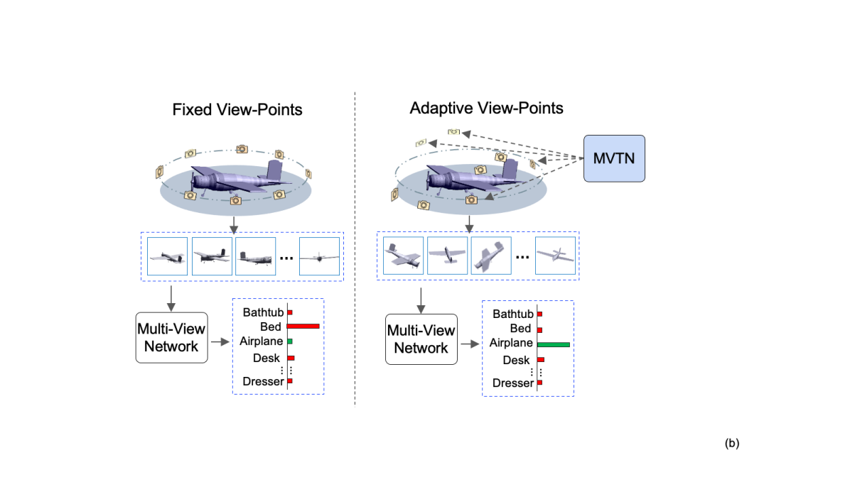
Figure 1: Multi-View Transformation Network (MVTN). We propose a differentiable module that predicts the best view-points for a task-specific multi-view network. MVTN is trained jointly with this network without any extra training supervision, while improving the performance on 3D classification and shape retrieval.

Recent multi-view methods have shown great performance in 3D shape classification and segmentation, often achieving state-of-the-art results [46, 81, 51, 45, 19]. These approaches use 2D convolutional architectures to solve 3D tasks by rendering multiple views of a given 3D shape and leveraging the rendered images. This allows them to build upon advances in 2D deep learning and make use of larger image datasets, such as ImageNet [73], to compensate for the lack of labeled 3D data. However, the choice of rendering view-points for these methods is often based on heuristics, such as random sampling [51] or predefined view-points, rather than being optimized for the task at hand. To address this issue, we propose the Multi-View Transformation Network (MVTN), which learns to regress suitable view-points for a given task and trains a downstream task-specific network in an end-to-end fashion using these views. As shown in Fig. 1, MVTN learns to regress view-points, renders those views with a differentiable renderer, and trains the downstream task-specific network in an end-to-end fashion, thus leading to the most suitable views for the task. This approach is inspired by the Spatial Transformer Network (STN) [40], which performs a similar function in the 2D image domain. Both MVTN and STN learn spatial transformations for the input without requiring additional supervision or adjustments to the learning process.

The concept of perception through the prediction of the best environment parameters that generated an image is known as Vision as Inverse Graphics (VIG) [30, 50, 84, 44, 92]. One approach to VIG is to make the rendering process invertible or differentiable [61, 47, 58, 16, 56]. In this paper, we use the Multi-View Transformation Network (MVTN) to take advantage of differentiable rendering [47, 58, 72] in order to train models end-to-end for a specific 3D vision task, with the view-points (i.e. camera poses) being inferred by MVTN in the same forward pass. To the best of our knowledge, we are the first to integrate a learnable approach to view-point prediction in multi-view methods by using a differentiable renderer and establishing an end-to-end pipeline that works for both mesh and 3D point cloud classification and retrieval.

Contributions: (1) We propose a Multi-View Transformation Network (MVTN) that regresses better view-points for multi-view methods. Our MVTN leverages a differentiable renderer that enables end-to-end training for 3D shape recognition tasks. (2) Combining MVTN with multi-view approaches leads to state-of-the-art results in 3D classification and shape retrieval on standard benchmarks ModelNet40 [85], ShapeNet Core55 [10, 74], and ScanObjectNN [78]. (3) Additional analysis shows that MVTN improves the robustness of multi-view approaches to rotation and occlusion. (4) We investigate an optimization alternative to MVTN, study different 2D pretraining strategies on MVTN, and study extending MVTN for 3D segmentation. To wrap up the work, we release MVTorch, a modular Pytroch library for multi-view research

A preliminary version of this work was published at ICCV 2021 [31]. This journal manuscript extends the initial version in several aspects. First, we investigate and experiment with a logical alternative to MVTN by treating the problem as an optimization of the scene parameters instead of learning a transformation network. Second, we study the effect of different pretraining strategies of the 2D backbone, which was shown in [31] to play an important role in MVTN’s success. Third, we extend MVTN to the 3D part segmentation task and show promise in learning views beyond classification pipelines. Finally, to ensure the reproducibility of our experiments and to contribute to the 3D understanding/generation research community, we have published MVTorch, a modular Pytorch library for training, testing, and visualization of multi-view deep learning pipelines.

2 Related Work

Deep Learning on 3D Data. PointNet [68] was the first deep learning algorithm to operate directly on 3D point clouds. It computed point features independently and aggregated them using an order invariant function such as max-pooling. Subsequent works focused on finding neighborhoods of points in order to define point convolutional operations [71, 80, 57, 53, 52, 79]. Voxel-based deep networks enable 3D CNNs, but they suffer from cubic memory complexity [63, 17, 29]. Some recent works have combined point cloud representations with other 3D modalities, such as voxels [60] or multi-view images [90, 41]. In this paper, we use a point encoder to predict optimal view-points, from which images are rendered and fed to a multi-view network.

Multi-View 3D Shape Classification. The use of 2D images to recognize 3D objects was first proposed by Bradski et al. [5]. Two decades later, MVCNN [75] emerged as the first application of deep 2D CNNs for 3D object recognition. MVCNN used max pooling to aggregate features from different views. Subsequent works proposed different strategies for assigning weights to views in order to perform weighted average pooling of view-specific features [91, 88, 24, 15]. RotationNet [46] classified views and objects jointly, while Equivariant MV-Network [22] used a rotation equivariant convolution operation on multiple views with rotation group convolutions [18]. ViewGCN [81] used dynamic graph convolution operations to adaptively pool features from fixed views for 3D shape classification. Previous methods relied on fixed rendered datasets of 3D objects. The work of [15] attempted to adaptively select views through reinforcement learning and RNNs, but it had limited success and required a complex training process. In this paper, we propose the Multi-View Transformation Network (MVTN) for predicting optimal view-points in a multi-view setup, by jointly training MVTN with a multi-view task-specific network without requiring any additional supervision or adjustments to the learning process.

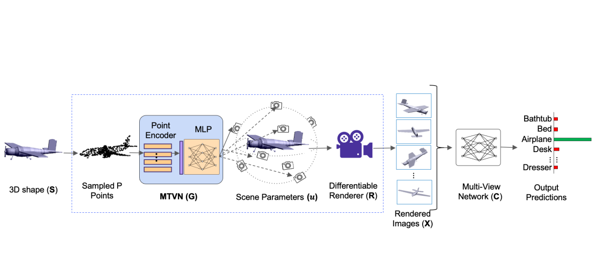
Figure 2: End-to-End Learning Pipeline for Multi-View Recognition. To learn adaptive scene parameters $\mathbf{u}$ that maximize the performance of a multi-view network $\mathbf{C}$ for every 3D object shape $\mathbf{S}$, we use a differentiable renderer $\mathbf{R}$. MVTN extracts coarse features from $\mathbf{S}$ by a point encoder and regresses the adaptive scene parameters for that object. In this example, the parameters $\mathbf{u}$ are the azimuth and elevation angles of cameras pointing towards the center of the object. The MVTN pipeline is optimized end-to-end for the task loss.

3D Shape Retrieval. Early methods in the literature compared the distribution of hand-crafted descriptors to retrieve similar 3D shapes. These shape signatures could represent either geometric [66] or visual [12] cues. Traditional geometric methods estimated the distributions of certain characteristics (such as distances, angles, areas, or volumes) to measure the similarity between shapes [1, 11, 7]. Gao et al. [26] used multiple camera projections, and Wu et al. [86] used a voxel grid to extract model-based signatures. Su et al. [75] introduced a deep learning pipeline for multi-view classification, with aggregated features achieving high retrieval performance. They used a low-rank Mahalanobis metric on top of extracted multi-view features to improve retrieval performance. This work on multi-view learning was extended for retrieval with volumetric-based descriptors [69], hierarchical view-group architectures [24], and triplet-center loss [38]. Jiang et al. [43] investigated better views for retrieval using many loops of circular cameras around the three principal axes. However, these approaches considered fixed camera view-points, as opposed to the learnable view-points of MVTN.

Vision as Inverse Graphics (VIG). A key challenge in Vision as Inverse Graphics (VIG) is the non-differentiability of the classical graphics pipeline. Recent VIG approaches have focused on making graphics operations differentiable, allowing gradients to flow directly from the image to the rendering parameters [61, 47, 58, 56, 16]. NMR [47] approximates non-differentiable rasterization by smoothing edge rendering, while SoftRas [58] assigns a probability for all mesh triangles to every pixel in the image. Synsin [82] proposes an alpha-blending mechanism for differentiable point cloud rendering. Pytorch3D [72] improves the speed and modularity of SoftRas and Synsin, and allows for customized shaders and point cloud rendering. MVTN takes advantage of these advances in differentiable rendering to jointly train with the multi-view network in an end-to-end fashion. By using both mesh and point cloud differentiable rendering, MVTN can work with 3D CAD models and more readily available 3D point cloud data

3 Methodology

We illustrate our proposed multi-view pipeline using MVTN in Fig. 2. MVTN is a generic module that learns camera view-point transformations for specific 3D multi-view tasks, e.g. 3D shape classification. In this section, we review a generic framework for common multi-view pipelines, introduce MVTN details, and present an integration of MVTN for 3D shape classification and retrieval.

3.1 Overview of Multi-View 3D Recognition

3D multi-view recognition defines $M$ different images $\{\mathbf{x}_{i}\}_{i=1}^{M}$ rendered from multiple view-points of the same shape $\mathbf{S}$. The views are fed into the same backbone network $\mathbf{f}$ that extracts discriminative features per view. These features are then aggregated among views to describe the entire shape and used for downstream tasks such as classification or retrieval. Specifically, a multi-view network $\mathbf{C}$ with parameters $\boldsymbol{\theta}_{\mathbf{C}}$ operates on an input set of images $\mathbf{X}\in\mathbb{R}^{M\times h\times w\times c}$ to obtain a softmax probability vector for the shape $\mathbf{S}$.

Training Multi-View Networks. The simplest deep multi-view classifier is MVCNN, where $\mathbf{C}=\text{MLP}\left(\max_{i}\mathbf{f}(\mathbf{x}_{i})\right)$ with $\mathbf{f}:\mathbb{R}^{h\times w\times c}\rightarrow{\mathbb{R}^{d}}$ being a 2D CNN backbone (e.g. ResNet [37]) applied individually on each rendered image. A more recent method like ViewGCN would be described as $\mathbf{C}=\text{MLP}\left(\text{cat}_{\text{GCN}}\left(\mathbf{f}(\mathbf{x}_{i})\right)\right)$, where $\text{cat}_{\text{GCN}}$ is an aggregation of views’ features learned from a graph convolutional network. In general, learning a task-specific multi-view network on a labeled 3D dataset is formulated as:

$$\operatorname*{arg\,min}_{\boldsymbol{\theta}_{\mathbf{C}}}~{}~{}\sum_{n}^{N}L~{}\big{(}\mathbf{C}(\mathbf{X}_{n})~{},~{}y_{n}\big{)}$$ (1)

$$={} \operatorname*{arg\,min}_{\boldsymbol{\theta}_{\mathbf{C}}}\sum_{n}^{N}L~{}\Big{(}\mathbf{C}\big{(}\mathbf{R}(\mathbf{S}_{n},\mathbf{u}_{0})\big{)}~{},~{}y_{n}\Big{)},$$

where $L$ is a task-specific loss defined over $N$ 3D shapes in the dataset, $y_{n}$ is the label for the $n^{\text{th}}$ 3D shape $\mathbf{S}_{n}$, and $\mathbf{u}_{0}\in\mathbb{R}^{\tau}$ is a set of $\tau$ fixed scene parameters for the entire dataset. These parameters represent properties that affect the rendered image, including camera view-point, light, object color, and background. $\mathbf{R}$ is the renderer that takes as input a shape $\mathbf{S}_{n}$ and the parameters $\mathbf{u}_{0}$ to produce $M$ multi-view images $\mathbf{X}_{n}$ per shape. In our experiments, we choose the scene parameters $\mathbf{u}$ to be the azimuth and elevation angles of the camera view-points pointing towards the object center, thus setting $\tau=2M$.

Canonical Views. Previous multi-view methods rely on scene parameters $\mathbf{u}_{0}$ that are pre-defined for the entire 3D dataset. In particular, the fixed camera view-points are usually selected based on the alignment of the 3D models in the dataset. The most common view configurations are circular that aligns view-points on a circle around the object [75, 91] and spherical that aligns equally spaced view-points on a sphere surrounding the object [81, 46]. Fixing those canonical views for all 3D objects can be misleading for some classes. For example, looking at a bed from the bottom could confuse a 3D classifier. In contrast, MVTN learns to regress per-shape view-points, as illustrated in Fig. 3.

3.2 Multi-View Transformation Network (MVTN)

Previous multi-view methods take the multi-view image $\mathbf{X}$ as the only representation for the 3D shape, where $\mathbf{X}$ is rendered using fixed scene parameters $\mathbf{u}_{0}$. In contrast, we consider a more general case, where $\mathbf{u}$ is variable yet within bounds $\pm\mathbf{u}_{\text{bound}}$. Here, $\mathbf{u}_{\text{bound}}$ is positive and it defines the permissible range for the scene parameters. We set $\mathbf{u}_{\text{bound}}$ to $180^{\circ}$ and $90^{\circ}$ for each azimuth and elevation angle.

Circular	Spherical	MVTN

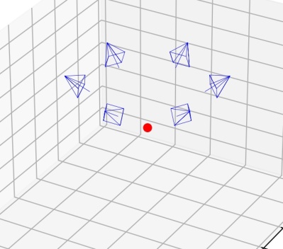
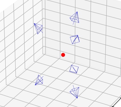
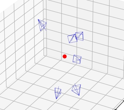
Figure 3: Multi-View Camera Configurations: The view setups commonly used in the multi-view literature are circular [75] or spherical [81, 46]. Our MVTN learns to predict specific view-points for each object shape at inference time. The shape’s center is shown as a red dot, and the view-points as blue cameras with their mesh renderings shown at the bottom.

Differentiable Renderer. A renderer $\mathbf{R}$ takes a 3D shape $\mathbf{S}$ (mesh or point cloud) and scene parameters $\mathbf{u}$ as inputs, and outputs the corresponding $M$ rendered images $\{\mathbf{x}_{i}\}_{i=1}^{M}$. Since $\mathbf{R}$ is differentiable, gradients $\frac{\partial\mathbf{x}_{i}}{\partial\mathbf{u}}{}$ can propagate backward from each rendered image to the scene parameters, thus establishing a framework that suits end-to-end deep learning pipelines. When $\mathbf{S}$ is represented as a 3D mesh, $\mathbf{R}$ has two components: a rasterizer and a shader. First, the rasterizer transforms meshes from the world to view coordinates given the camera view-point and assigns faces to pixels. Using these face assignments, the shader creates multiple values for each pixel then blends them. On the other hand, if $\mathbf{S}$ is represented by a 3D point cloud, $\mathbf{R}$ would use an alpha-blending mechanism instead [82]. Fig. 3 and Fig. 4 illustrate examples of mesh and point cloud renderings used in MVTN.

View-Points Conditioned on 3D Shape. We design $\mathbf{u}$ to be a function of the 3D shape by learning a Multi-View Transformation Network (MVTN), denoted as $\mathbf{G}\in\mathbb{R}^{P\times 3}\rightarrow{\mathbb{R}^{\tau}}$ and parameterized by $\boldsymbol{\theta}_{\mathbf{G}}$, where $P$ is the number of points sampled from shape $\mathbf{S}$. Unlike Eq (1) that relies on constant rendering parameters, MVTN predicts $\mathbf{u}$ adaptively for each object shape $\mathbf{S}$ and is optimized along with the classifier $\mathbf{C}$. The pipeline is trained end-to-end to minimize the following loss on a dataset of N objects:

$$\operatorname*{arg\,min}_{\boldsymbol{\theta}_{\mathbf{C}},\boldsymbol{\theta}_{\mathbf{G}}} \sum_{n}^{N}L~{}\Big{(}\mathbf{C}\big{(}\mathbf{R}(\mathbf{S}_{n},\mathbf{u}_{n})\big{)}~{},~{}y_{n}\Big{)},$$ (2)

$$\text{s. t.}\quad\mathbf{u}_{n}=~{}\mathbf{u}_{\text{bound}}.\text{tanh}\big{(}\mathbf{G}(\mathbf{S}_{n})\big{)}$$

Here, $\mathbf{G}$ encodes a 3D shape to predict its optimal view-points for the task-specific multi-view network $\mathbf{C}$. Since the goal of $\mathbf{G}$ is only to predict view-points and not classify objects (as opposed to $\mathbf{C}$), its architecture is designed to be simple and light-weight. As such, we use a simple point encoder (e.g. shared MLP as in PointNet [68]) that processes $P$ points from $\mathbf{S}$ and produces coarse shape features of dimension $b$. Then, a shallow MLP regresses the scene parameters $\mathbf{u}_{n}$ from the global shape features. To force the predicted parameters $\mathbf{u}$ to be within a permissible range $\pm\mathbf{u}_{\text{bound}}$, we use a hyperbolic tangent function scaled by $\mathbf{u}_{\text{bound}}$.

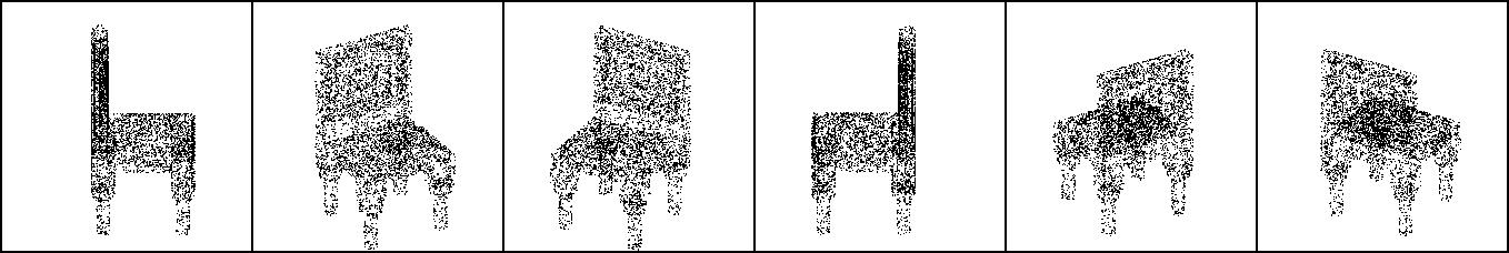
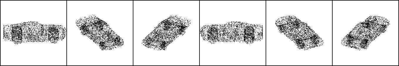
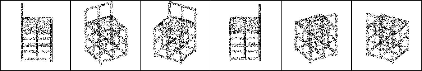
Figure 4: Multi-View Point Cloud Renderings. We show some examples of point cloud renderings used in our pipeline. Note how point cloud renderings offer more information about content hidden from the camera view-point (e.g. car wheels from the occluded side), which can be useful for recognition.

MVTN for 3D Shape Classification. To train MVTN for 3D shape classification, we define a cross-entropy loss in Eq (2), yet other losses and regularizers can be used here as well. The multi-view network ($\mathbf{C}$) and the MVTN ($\mathbf{G}$) are trained jointly on the same loss. One merit of our multi-view pipeline is its ability to seamlessly handle 3D point clouds, which is absent in previous multi-view methods. When $\mathbf{S}$ is a 3D point cloud, we simply define $\mathbf{R}$ as a differentiable point cloud renderer.

MVTN for 3D Shape Retrieval. The shape retrieval task is defined as follows: given a query shape $\mathbf{S}_{q}$, find the most similar shapes in a broader set of size $N$. For this task, we follow the retrieval setup of MVCNN [75]. In particular, we consider the deep feature representation of the last layer before the classifier in $\mathbf{C}$. We project those features into a more expressive space using LFDA reduction [76] and consider the reduced feature as the signature to describe a shape. At test time, shape signatures are used to retrieve (in order) the most similar shapes in the training set.

4 Experiments

We evaluate MVTN for the tasks of 3D shape classification and retrieval on ModelNet40 [85], ShapeNet Core55 [10], and the more realistic ScanObjectNN [78].

4.1 Datasets

ModelNet40. The ModelNet40 dataset [85] consists of 12,311 3D objects with 40 object classes, with a split of 9,843 objects in the training set and 2,468 in the testing set. Due to hardware limitations, the meshes in this dataset have been simplified to 20,000 vertices using the official Blender API [4, 27].

ShapeNet Core55. The ShapeNet Core55 dataset [10] is a subset of ShapeNet comprising 51,162 3D mesh objects with 55 object classes. It was created for the shape retrieval challenge SHREK [74] and includes 35764 objects in the training set, 5133 in the validation set, and 10265 in the test set.

ScanObjectNN. The ScanObjectNN dataset [78] is a more realistic and challenging point cloud dataset for 3D classification, including background and occlusions. It consists of 2,902 point clouds divided into 15 object categories and has three main variants: object only, object with background, and the hardest perturbed variant (PB_T50_RS variant). These variants are used in the 3D Scene Understanding Benchmark associated with the ScanObjectNN dataset and offer a more challenging evaluation of the generalization capabilities of 3D deep learning models in realistic scenarios compared to ModelNet40.

4.2 Metrics

Classification Accuracy. The standard evaluation metric in 3D classification is accuracy. We report overall accuracy (percentage of correctly classified test samples) and average per-class accuracy (mean of all true class accuracies).

Retrieval mAP. Shape retrieval is evaluated by mean Average Precision (mAP) over test queries. For every query shape $\mathbf{S}_{q}$ from the test set, AP is defined as $AP=\frac{1}{\text{GTP}}\sum_{n}^{N}\frac{\mathbbm{1}(\mathbf{S}_{n})}{n}$, where $GTP$ is the number of ground truth positives, $N$ is the size of the ordered training set, and $\mathbbm{1}(\mathbf{S}_{n})=1$ if the shape $\mathbf{S}_{n}$ is from the same class label of query $\mathbf{S}_{q}$. We average the retrieval AP over the test set to measure retrieval mAP.

4.3 Baselines

Voxel Networks. We choose VoxNet [63], DLAN [25], and 3DShapeNets [85] as baselines that use voxels.

Point Cloud Networks. We select PointNet [68], PointNet++ [71], DGCNN [80], PVNet [90], and KPConv [77] as baselines that use point clouds. These methods leverage different convolution operators on point clouds by aggregating local and global point information.

Multi-view Networks. We compare against MVCNN [75], RotationNet [46], GVCNN [24] and ViewGCN [81] as representative multi-view methods. These methods are limited to meshes, pre-rendered from canonical view-points.

4.4 MVTN Details

Rendering. In our pipeline, we utilize the differentiable mesh and point cloud renderers from Pytorch3D [72] for their compatibility with Pytorch libraries [67] and fast processing speed. Examples of rendered images for meshes and point clouds can be seen in Figures 3 and 4, respectively. Each rendered image has a size of 224$\times$224. For ModelNet40, we utilize the differentiable mesh renderer and apply augmentation during training by randomly directing the light and assigning a random color to the object. In testing, we fix the light direction towards the center of the object and color the object white for stable performance. For ShapeNet Core55 and ScanObjectNN, we use the differentiable point cloud renderer with 2048 and 5000 points, respectively. The use of a point cloud renderer offers a lighter alternative to mesh rendering when the mesh contains a large number of faces, which can hinder the training of the MVTN pipeline.

		Classification Accuracy
Method	Data Type	(Per-Class)	(Overall)
VoxNet [63]	Voxels	83.0	85.9
PointNet [68]	Points	86.2	89.2
PointNet++ [71]	Points	-	91.9
PointCNN [57]	Points	88.1	91.8
DGCNN [80]	Points	90.2	92.2
KPConv[77]	Points	-	92.9
MVCNN [75]	12 Views	90.1	90.1
GVCNN [24]	12 Views	90.7	93.1
ViewGCN [81]	20 Views	96.5	97.6
ViewGCN [81]∗	12 views	90.7	93.0
ViewGCN [81]∗	20 views	91.3	93.3
MVTN (ours)∗	12 Views	92.0	93.8
MVTN (ours)∗	20 Views	92.2	93.5

TABLE I: 3D Shape Classification on ModelNet40. We compare MVTN against other methods in 3D classification on ModelNet40 [85]. ^∗ indicates results from our rendering setup (differentiable pipeline), while other multi-view results are reported from pre-rendered views. Bold denotes the best result in its setup.

	Classification Overall Accuracy
Method	OBJ_BG	OBJ_ONLY	Hardest
3DMFV [3]	68.2	73.8	63.0
PointNet [68]	73.3	79.2	68.0
SpiderCNN [87]	77.1	79.5	73.7
PointNet ++ [71]	82.3	84.3	77.9
PointCNN [57]	86.1	85.5	78.5
DGCNN [80]	82.8	86.2	78.1
SimpleView [28]	-	-	79.5
BGA-DGCNN [78]	-	-	79.7
BGA-PN++ [78]	-	-	80.2
MVTN (ours)	92.6	92.3	82.8

TABLE II: 3D Point Cloud Classification on ScanObjectNN. We compare the performance of MVTN in 3D point cloud classification on three different variants of ScanObjectNN [78]. The variants include object with background, object only, and the hardest variant.

View-Point Prediction. As shown in Eq (2), the MVTN $\mathbf{G}$ network learns to predict the view-points directly (MVTN-direct). Alternatively, MVTN can learn relative offsets w.r.t. initial parameters $\mathbf{u}_{0}$. In this case, we concatenate the point features extracted in $\mathbf{G}$ with $\mathbf{u}_{0}$ to predict the offsets to apply on $\mathbf{u}_{0}$. The learned view-points $\mathbf{u}_{n}$ in Eq (2) are defined as: $~{}\mathbf{u}_{n}=\mathbf{u}_{0}+\mathbf{u}_{\text{bound}}.\text{tanh}\big{(}\mathbf{G}(\mathbf{u}_{0}~{},~{}\mathbf{S}_{n})\big{)}$. We take $\mathbf{u}_{0}$ to be the circular or spherical configurations commonly used in multi-view classification pipelines [75, 46, 81]. We refer to these learnable variants as MVTN-circular and MVTN-spherical, accordingly. For MVTN-circular, the initial elevations for the views are 30^∘, and the azimuth angles are equally distributed over 360^∘ following [75]. For MVTN-spherical, we follow the method from [20] that places equally-spaced view-points on a sphere for an arbitrary number of views, which is similar to the “dodecahedral” configuration in ViewGCN.

		Shape Retrieval (mAP)
Method	Data Type	ModelNet40	ShapeNet Core
DLAN [25]	Voxels	-	66.3
LFD [13]	Voxels	40.9	-
3D ShapeNets [85]	Voxels	49.2	-
PVNet[90]	Points	89.5	-
MVCNN [75]	12 Views	80.2	73.5
GIFT [2]	20 Views	-	64.0
MVFusionNet [42]	12 Views	-	62.2
ReVGG [74]	20 Views	-	74.9
RotNet [46]	20 Views	-	77.2
ViewGCN [81]	20 Views	-	78.4
MLVCNN [43]	24 Views	92.2	-
MVTN (ours)	12 Views	92.9	82.9

TABLE III: 3D Shape Retrieval. We benchmark the shape retrieval mAP of MVTN on ModelNet40 [85] and ShapeNet Core55 [10, 74]. MVTN achieves the best retrieval performance among recent state-of-the-art methods on both datasets with only 12 views.

Architecture. In our MVTN pipeline, we select MVCNN [75] and ViewGCN [81] as our multi-view networks of choice. In our experiments, we use PointNet [68] as the 3D point encoder network $\mathbf{G}$ and experiment with DGCNN in Section 6.1. We sample 2048 points from each mesh as input to the point encoder and use a 5-layer MLP for the regression network, which takes as input the point features extracted by the point encoder of size $b=40$. All MVTN variants and the baseline multi-view networks utilize a ResNet-18 [37] network, pretrained on ImageNet [73], as the multi-view backbone in $\mathbf{C}$, with output features of size $d=1024$. The main classification and retrieval results are based on MVTN-spherical with ViewGCN [81] as the multi-view network $\mathbf{C}$, unless otherwise specified in Section 5.3 and 6.1.

Training Setup. To avoid gradient instability introduced by the renderer, we use gradient clipping in the MVTN network $\mathbf{G}$. We clip the gradient updates such that the $\ell_{2}$ norm of the gradients does not exceed 30. We use a learning rate of $0.001$ but refrain from fine-tuning the hyper-parameters introduced in MVCNN  [75] and View-GCN [81]. More details about the training procedure are in the supplementary material .

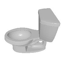
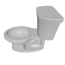
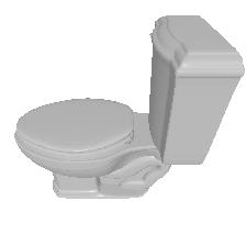
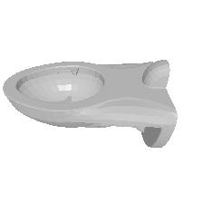
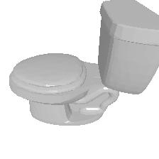
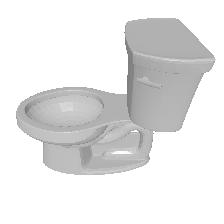
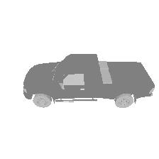
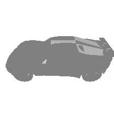
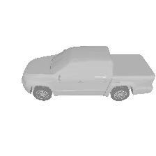
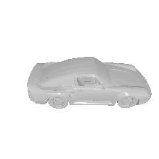
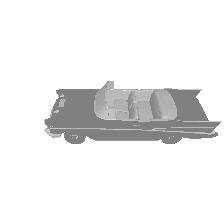
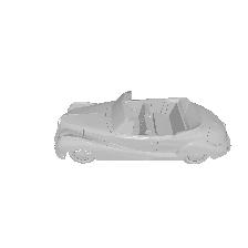
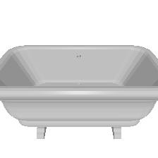
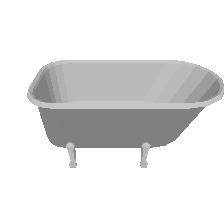
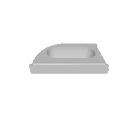
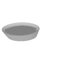
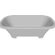
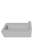
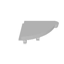
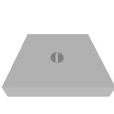
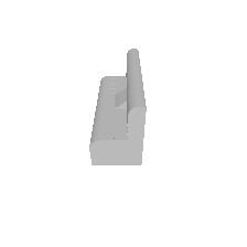
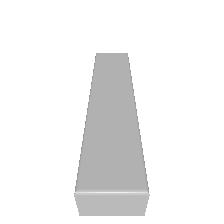
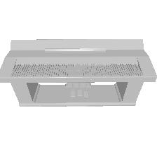
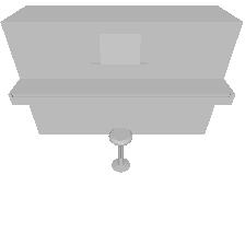
Figure 5: Qualitative Examples for Object Retrieval: (left): we show some query objects from the test set. (right): we show top five retrieved objects by our MVTN from the training set. Images of negative retrieved objects are framed.

5 Results

The main results of MVTN are summarized in Tables I, II, III and IV. We achieve state-of-the-art performance in 3D classification on ScanObjectNN by a large margin (up to 6%) and achieve a competitive test accuracy of 93.8% on ModelNet40. On shape retrieval, we achieve state-of-the-art performance on both ShapeNet Core55 (82.9 mAP) and ModelNet40 (92.9 mAP). Following the common practice, we report the best results out of four runs in benchmark tables, but detailed results are in supplementary material .

5.1 3D Shape Classification

Table I compares the performance of MVTN against other methods on ModelNet40 [85]. Our MVTN achieves a competitive test accuracy of 93.8% compared to all previous methods. ViewGCN [81] achieves higher classification performance by relying on higher quality images from a more advanced yet non-differentiable OpenGL [83] renderer. For a fair comparison, we report with an ^∗ the performance of ViewGCN using images generated by the renderer used in MVTN. Using the same rendering process, regressing views with MVTN improves the classification performance of the baseline ViewGCN at 12 and 20 views. We believe future advances in differentiable rendering would bridge the gap between our rendered images and the original high-quality pre-rendered ones.

Table II reports the classification accuracy of a 12 view MVTN on the realistic ScanObjectNN benchmark [78]. MVTN improves performance on different variants of the dataset. The most difficult variant of ScanObjectNN (PB_T50_RS) includes challenging scenarios of objects undergoing translation and rotation. Our MVTN achieves state-of-the-art results (+2.6%) on this variant, highlighting the merits of MVTN for realistic 3D point cloud scans. Also, note how adding background points (in OBJ_BG) does not hurt MVTN, contrary to most other classifiers. .

5.2 3D Shape Retrieval

Table III presents the retrieval mean average precision (mAP) of MVTN compared to recent methods on ModelNet40 [85] and ShapeNet Core55 [10]. The results for the latter methods are taken from [43, 81, 90]. MVTN demonstrates state-of-the-art retrieval performance, achieving a mAP of 92.9% on ModelNet40. It also significantly improves upon the state-of-the-art on ShapeNet, using only 12 views. It is worth noting that the baselines in Table III include strong, recently developed methods specifically trained for retrieval, such as MLVCNN [43]. Fig. 5 shows qualitative examples of objects retrieved using MVTN.

	Rotation Perturbations Range
Method	$0^{\circ}$	$\pm 90^{\circ}$	$\pm 180^{\circ}$
PointNet [68]	88.7	42.5	38.6
PointNet ++ [71]	88.2	47.9	39.7
RSCNN [59]	90.3	90.3	90.3
MVTN (ours)	91.7	90.8	91.2

TABLE IV: Rotation Robustness on ModelNet40. At test time, we randomly rotate objects in ModelNet40 around the Y-axis (gravity) with different ranges and report the overall accuracy. MVTN displays strong robustness to such Y-rotations.

5.3 Rotation Robustness

Evaluating the robustness of trained models to perturbations at test time is a common practice in the 3D shape classification literature. Following the same procedure as [59, 33], we perturb the shapes with random rotations around the Y-axis (gravity-axis) within the range of $\pm 90^{\circ}$ and $\pm 180^{\circ}$. We repeat the inference process ten times for each setup and report the average performance in Table IV. The MVTN-circular variant (using MVCNN) achieves state-of-the-art performance in rotation robustness (91.2% test accuracy) compared to more advanced methods trained in the same setup. The baseline method, RSCNN [59], is a strong model designed to be invariant to translation and rotation, while MVTN is learned in a simpler setup using MVCNN without targeting rotation invariance.

5.4 Occlusion Robustness

To assess the practical usefulness of MVTN in realistic scenarios, we investigate the problem of occlusion in 3D computer vision, particularly in 3D point cloud scans. Occlusion can be caused by various factors, such as the view angle to the object, the sampling density of the sensor (e.g., LiDAR), or the presence of noise in the sensor. In these realistic scenarios, deep learning models often struggle. To evaluate the effect of occlusion due to the viewing angle of the 3D sensor in our 3D classification setup, we simulate realistic occlusion by cropping the object from canonical directions. We train PointNet [68], DGCNN [80], and MVTN on the ModelNet40 point cloud dataset, and then crop a portion of the object (from 0% occlusion to 100%) along the $\pm$X, $\pm$Y, and $\pm$Z directions at test time. Fig. 6 illustrates examples of this occlusion effect at different occlusion ratios. Table V reports the average test accuracy of the six cropping directions for the baselines and MVTN. MVTN exhibits high test accuracy even when large portions of the object are cropped. In fact, MVTN outperforms PointNet [68] by 13% in test accuracy when half of the object is occluded, despite PointNet’s reputation for robustness [68, 34]. This result highlights the effectiveness of MVTN in handling occlusion.

	Occlusion Ratio
dir.	0.1	0.2	0.3	0.5	0.75
+X
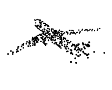
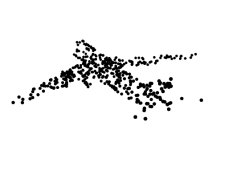
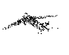
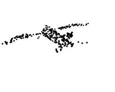
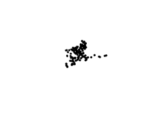
-X
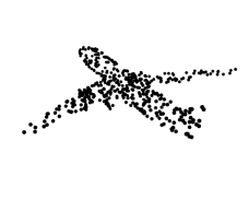
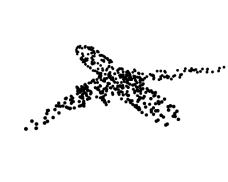
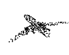
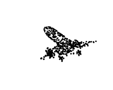
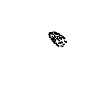
+Y
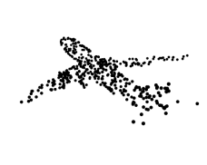
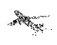
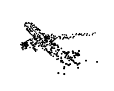
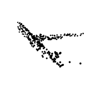
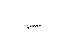
-Y

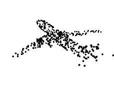
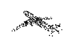
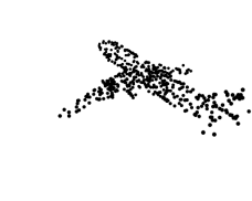
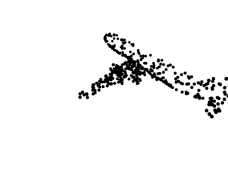
Figure 6: Occlusion of 3D Objects: We simulate realistic occlusion scenarios in 3D point clouds by cropping a percentage of the object along canonical directions. Here, we show an object occluded with different ratios and from different directions.

	Occlusion Ratio
Method	0	0.1	0.2	0.3	0.5	0.75
PointNet [68]	89.1	88.2	86.1	81.6	53.5	4.7
DGCNN [80]	92.1	77.1	74.5	71.2	30.1	4.3
MVTN (ours)	92.3	90.3	89.9	88.3	67.1	9.5

TABLE V: Occlusion Robustness of 3D Methods. We report the test accuracy on point cloud ModelNet40 for different occlusion ratios of the data to measure occlusion robustness of different 3D methods. MVTN achieves 13% better accuracy than PointNet (a robust network) when half of the object is occluded.

5.5 Optimizing Scene Parameters

As an alternative to MVTN that leverages the end-to-end differentiable pipeline, we can treat the view selection problem as an optimization objective for scene parameters instead of learning a network. To do this, we experiment with optimizing the azimuth and elevation angles used for rendering during training by either maximizing or minimizing the Cross-Entropy (CE) loss while the main multi-view network is training. To accomplish this, we run a varying number of iterations for each batch in training, during which we render the input scene parameters, calculate the loss, and update the parameters using SGD. We test whether this optimization will outperform the baseline model without learning views and the baseline model with random noise added to the input view parameters. We also try minimizing and maximizing the norm of the rendered images, which decreases or increases coverage, respectively (Coverage Loss). Additionally, we attempt to maximize the distance between the top two logits from the output of the images (Adversarial Loss [8]). The CE loss optimization is only applied during training, while the coverage and adversarial losses are optimized during both training and test time.

Initial Setup. We use the regular pipeline without learning views, a batch size of 20, 8 spherical views, black backgrounds, and white point cloud renderings to train on the three variants of the ScanObjectNN [78] dataset. We optimize MVCNN [75] using AdamW [62] and a learning rate of 0.001, and use ResNet-18 [37] as the backbone CNN. The baseline with noise adds a sample drawn from a normal distribution with a mean of 0 and standard deviation of 18 to each azimuth angle, and a mean of 0 and standard deviation of 9 to the elevation angles.

Optimization Results. To determine the optimal parameters for our optimization approach, we test different numbers of optimization iterations for each batch and various values for the learning rate. We also try using a ResNet-18 [37] backbone that is either pretrained or not pretrained. We find that the best results are obtained with a pretrained backbone, a learning rate of 50, and 10 optimization iterations using the cross entropy loss. For the coverage and adversarial losses, we use a pretrained backbone, a learning rate of 25, and 10 optimization iterations. The results are presented in Table VI.

	Classification Overall Accuracy
Method	OBJ_BG	OBJ_ONLY	Hardest
Baseline Without Noise	85.42	84.56	72.83
Baseline With Noise	85.59	84.56	78.52
Maximizing CE Loss	83.53	86.28	74.95
Minimizing CE Loss	84.91	85.08	75.19
Maximizing Coverage Loss	86.28	85.25	75.75
Minimizing Coverage Loss	84.73	85.08	74.39
Maximizing Adversarial Loss	86.11	85.42	76.89

TABLE VI: Input Scene Parameters Optimization. We show the classification accuracy utilizing input scene optimization strategy using the different methods on the three ScanObjectNN [78] variants. The optimization methods either maximize or minimize different losses, and we compare them to the baseline fixed spherical models with and without added parameter noise.

6 Analysis and Insights

6.1 Ablation Study

This section performs a comprehensive ablation study on the different components of MVTN and their effect on the overall test accuracy on ModelNet40 [85].

Number of Views. We study the effect of the number of views $M$ on the performance of MVCNN when using fixed views (circular/spherical), learned views (MVTN), and random views. The experiments are repeated four times, and the average test accuracies with confidence intervals are shown in Fig. 7. The plots show how learned MVTN-spherical achieves consistently superior performance across a different number of views.

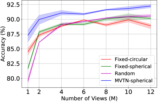
Figure 7: Effect of the Number of Views. We plot the test accuracy vs. the number of views (M) used to train MVCNN on fixed, random, and learned MVTN view configurations. We observe a consistent 2% improvement with MVTN over a variety of views.

Choice of Backbone and Point Encoders. Throughout our main MVTN experiments, we use ResNet-18 as the backbone and PointNet as the point feature extractor. However, different choices could be made for both. We investigate the use of DGCNN [80] as an alternative point encoder and ResNet-34 as an alternative 2D backbone in ViewGCN. The results of these ablation studies are presented in Table VII. We observe that using more complex CNN backbones and shape feature extractors in the MVTN setup does not significantly improve the results, which justifies our use of the simpler combination in our main experiments.

Late Fusion. In the MVTN pipeline, we use a point encoder and a multi-view network. One can argue that an easy way to combine them would be to fuse them later in the architecture. For example, PointNet [68] and MVCNN [75] can be max pooled together at the last layers and trained jointly. We train such a setup and compare it to MVTN. We observe that MVTN achieves $91.8\%$ compared to $88.4\%$ by late fusion.

Effect of Object Color. Our main experiments used random colors for the objects during training and fixed them to white in testing. We tried different coloring approaches, like using a fixed color during training and test. The results are illustrated in Table VIII.

Other Factors Affecting MVTN. We study the effect of the light direction in the renderer and the camera’s distance to the object. We also study the transferability of the learned views from one multi-view network to another, and the performance of MVTN variants. More details are provided in the supplementary material .

6.2 Visualizing MVTN Learned Views

In Fig. 8, we visualize the distribution of views predicted by MVTN for shapes from three different object classes. We use the MVTN-direct variant with $M=1$ to study the behavior of a single view. We histogram the learned views for the entire test set of ModelNet40. In this setups, we observe that MVTN is learning a per-instance view and not regressing the same view for shapes belonging to the same class. We see from Fig. 8 that the distribution of the MVTN views varies from one class to another, and the views from the same class exhibit some variance between instances.

Backbone	Point	MVTN	Results
Network	Encoder	Setup	Accuracy
ResNet-18	PointNet	circular	92.83 $\pm$ 0.06
		spherical	93.41 $\pm$ 0.13
	DGCNN	circular	93.03 $\pm$ 0.15
		spherical	93.26 $\pm$ 0.04
ResNet-34	PointNet	circular	92.72 $\pm$ 0.16
		spherical	92.83 $\pm$ 0.12
	DGCNN	circular	92.72 $\pm$ 0.03
		spherical	92.63 $\pm$ 0.15

TABLE VII: Ablation Study. We analyze the effect of ablating different MVTN components on test accuracy in ModelNet40. Namely, we observe that using deeper backbone CNNs or a more complex point encoder do not increase the test accuracy.

	Object Color
Method	White	Random
Fixed views	92.8 $\pm$ 0.1	92.8 $\pm$ 0.1
MVTN (learned)	93.3 $\pm$ 0.1	93.4 $\pm$ 0.1

TABLE VIII: Effect of Color Selection. We ablate selecting the color of the object in training our MVTN and when views are fixed in the spherical configuration. Fixed white color is compared to random colors in training. Note how randomizing the color helps in improving the test accuracy on ModelNet40 a little bit.

Probability Density

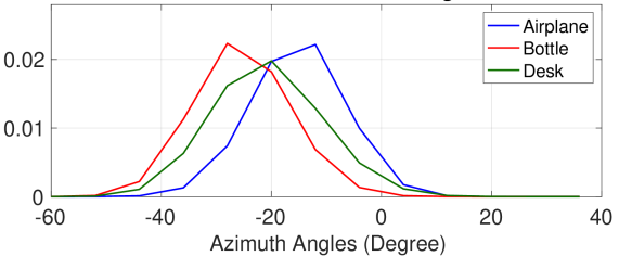
Figure 8: Visualizing MVTN Learned Views. We visualize the distribution of azimuth angles predicted by MVTN for three different classes. Note that MVTN learns inter-class variations (between different classes) and intra-class variations (in the same class).

6.3 2D Pretraining Strategy

We aim to evaluate the impact of 2D pretraining on the performance of our pipeline. We focus on two pretraining paradigms: Self-Supervised pretraining (SSL) and Full-Supervised pretraining (FSL). We conduct experiments using MVTN with ResNet-50 [37] and ViT [21] as backbone networks, starting from scratch or using weights from ImageNet [73], Dino [9], and Masked Autoencoders (MAE) [36] as initial weights. We also test FSL as pretraining for our model setup.

Experiment Setup. Using 8 learned spherical views, batch size of 20, black backgrounds, and white point cloud renderings. We train for 100 epochs using ResNet-50 [37] and ViT [21] on the three variants of the ScanObjectNN [78] dataset. For each backbone network, we run training from scratch without pretraining, and we run experiments with different pretraining methods. The pretraining methods include using ImageNet [73] weights and using SSL weights from Dino [9], and MAE [36]. For FSL pretraining, we first train for 100 epochs from scratch using 1 random view of each shape in the dataset and then use the resulting weights as our initial weights in the experiment setup mentioned before.

Results. The results of these experiments can be found in Tables IX and X for ViT [21] and ResNet-50 [37], respectively.

	Classification Overall Accuracy
Method	OBJ_BG	OBJ_ONLY	Hardest
Scratch ViT	68.78	75.47	61.97
ImageNet ViT	91.25	90.74	84.21
Dino ViT	90.91	91.08	81.37
MAE ViT	86.11	88.34	80.85
FSL ViT	62.61	71.18	57.53

TABLE IX: Effect of ViT Pretraining Strategy on MVTN. We show the impact of using different pretraining methods when training MVTN with ViT [21] as the backbone network.

	Classification Overall Accuracy
Method	OBJ_BG	OBJ_ONLY	Hardest
Scratch ResNet-50	63.64	71.01	61.21
ImageNet ResNet-50	88.16	89.02	81.26
Dino ResNet-50	81.13	84.39	77.69
FSL ResNet-50	58.66	65.18	52.22

TABLE X: Effect of ResNet50 Pretraining Strategy on MVTN. We show the impact of using different pretraining methods when training MVTN with ResNet-50 [37] as the backbone network.

6.4 MVTN for Part Segmentation

Experiment Setup. We investigate applying MVTN for part segmentation on ShapeNet Parts [89]. Similar to Voint Cloud [32], we use DeepLabV3 [14] as the 2D backbone and follow similar procedures in uplifting the predictions from 2D to 3D (mode un-projection). We add MVTN before the rendering process and optimize the MVTN network controlling the azimuth and elevation angles as before but using the 2D segmentation loss instead of the classification loss.

Results. The results for segmentation instance mean IOU of the pipeline with MVTN and without MVTN are reported in Fig. 9. It shows that as the number of views increases, the performance increase for both the baseline and MVTN, with marginal improvement using MVTN. Similar to the classification case, as the number of views becomes large, the margin of MVTN improvement becomes smaller.

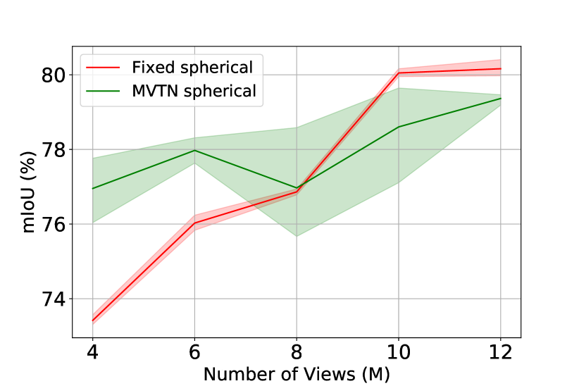
Figure 9: MVTN for Part Segmentation. We plot the 3D segmentation Instance mIOU vs. the number of views used in training the pipeline.

6.5 Time and Memory of MVTN

In this study, we evaluated the impact of the MVTN module on the time and memory requirements of our pipeline. To do this, we measured the number of floating point operations (FLOPs) and multiply-accumulate (MAC) operations for each module, as well as the time required for a single input sample to pass through each module and the number of parameters for each module. Our results, presented in Table XI, show that the MVTN module has a negligible impact on the overall time and memory requirements of the multi-view networks and 3D point encoders.

Network	FLOPs	MACs	Params. #	Time
PointNet	1.78 G	0.89 G	3.49 M	3.34 ms
DGCNN	10.42 G	5.21 G	0.95 M	16.35 ms
MVCNN	43.72 G	21.86 G	11.20 M	39.89 ms
ViewGCN	44.19 G	22.09 G	23.56 M	26.06 ms
MVTN∗	18.52 K	9.26 K	9.09 K	0.9 ms
MVTN∘	1.78 G	0.89 G	4.24 M	3.50 ms

TABLE XI: Time and Memory Requirements. We assess the contribution of the MVTN module to time and memory requirements in the multi-view pipeline. MVTN^∗ refers to MVTN’s regressor excluding the point encoder, while MVTN^∘ refers to the full MVTN module including PointNet as a point encoder.

6.6 MVTorch: a Library for Multi-view Deep Learning Research

We propose MVTorch, a PyTorch library that enables efficient, modular development of multi-view 3D computer vision and graphics research. This library is built using PyTorch [67] and Pytorch3D [72] and offers a variety of features for working with 3D data and multi-view images. These features include the ability to render differentiable multi-view images from 3D meshes and point clouds, data loaders for 3D data and multi-view images, visualizations of 3D meshes, point clouds, and multi-view images, modular training of multi-view networks for different 3D tasks, and input/output capabilities for 3D data and multi-view images. These features are implemented using PyTorch tensors and are designed to be used with mini-batches of heterogeneous data, allowing them to be easily differentiated and run on GPUs for acceleration.

Module	Time (ms)	Params (M)	GFLOPs
MVRenderer Points 4-V	10.74	0.00	-
MVRenderer Points 6-V	12.61	0.00	-
MVRenderer Points 8-V	15.42	0.00	-
MVRenderer Points 10-V	17.45	0.00	-
MVRenderer Points 12-V	20.16	0.00	-
MVRenderer Meshes 4-V	19.15	0.00	-
MVRenderer Meshes 6-V	25.11	0.00	-
MVRenderer Meshes 8-V	28.83	0.00	-
MVRenderer Meshes 10-V	32.94	0.00	-
MVRenderer Meshes 12-V	37.55	0.00	-
MVCNN ResNet-18 4-V	2.59	11.20	14.57
MVCNN ResNet-18 6-V	2.75	11.20	21.86
MVCNN ResNet-18 8-V	3.13	11.20	29.15
MVCNN ResNet-18 10-V	3.50	11.20	36.43
MVCNN ResNet-18 12-V	4.01	11.20	43.72
MVTN PointNet 4-V	3.46	3.47	1.77
MVTN PointNet 6-V	3.44	3.47	1.77
MVTN PointNet 8-V	3.46	3.47	1.77
MVTN PointNet 10-V	3.44	3.48	1.77
MVTN PointNet 12-V	3.42	3.48	1.77
MVTN DGCNN 4-V	4.09	0.95	10.42
MVTN DGCNN 6-V	4.10	0.96	10.42
MVTN DGCNN 8-V	4.10	0.96	10.42
MVTN DGCNN 10-V	4.10	0.96	10.42
MVTN DGCNN 12-V	4.10	0.96	10.42
MVPartSeg deeplab 4-V	54.00	61.00	387.74
MVPartSeg deeplab 6-V	67.15	61.00	581.61
MVPartSeg deeplab 8-V	91.04	61.00	775.48
MVPartSeg deeplab 10-V	112.52	61.00	969.35
MVPartSeg deeplab 12-V	121.49	61.00	1163.21

TABLE XII: Performance Benchmarking of MVTorch. We show different pipelines and configurations of the modules in MVtorch with the speed and compute cost associated with them on a varying number of views. The first block includes only the rendering pipeline. The second and third blocks are for 3D classification using MVCNN [75] with and without MVTN respectively. The last block is for the segmentation pipeline with DeepLabV3 [14].

Tutorials and documentation for MVTorch can be found on the project’s GitHub page (github.com/ajhamdi/mvtorch). his documentation includes examples of how to use MVTorch for tasks such as 3D classification, retrieval, segmentation, and generating 3D meshes from text [64], and Neural Radiance Fields [65] examples. Key classes in MVTorch include MVRenderer (for rendering both point clouds and meshes), MVNetwork (which allows any 2D network to be input and outputs its multi-view version), visualizer (for handling multi-view and 3D visualization), MVDataloader (for loading any dataset including ModelNet, ShapeNet, ScanObjectNN, ShapeNet Parts, and S3DIS), view-selector (e.g. MVTN, random, circular, etc.), and MVAggregate, which aggregates multi-view data into 3D representations (such as through maxpooling, meanpooling, point aggregation, and lifting). Table XII shows the performance of different modules and configurations in MVTorch for classification and segmentation tasks.

7 Conclusions

Current multi-view methods rely on fixed views aligned with the dataset. We propose MVTN that learns to regress view-points for any multi-view network in a fully differentiable pipeline. MVTN harnesses recent developments in differentiable rendering and does not require any extra training supervision. Empirical results highlight the benefits of MVTN in 3D classification and 3D shape retrieval.

Abdullah Hamdi Abdullah is a Ph.D. candidate in Electrical and Computer Engineering in Prof. Bernard Ghanem’s Computer Vision group at KAUST. He focuses on developing robust 3D computer vision techniques and tackling the adversarial robustness of deep neural networks. Abdullah has won a “best paper award” at the European Conference of Computer Vision ECCV 2020 and the NEOM AI Challenge 2020, among other national and international distinctions (AAI 2020, ECCV2020, and ICCV 2021). Abdullah is a regular reviewer for top computer vision and machine learning venues (CVPR, ICCV, ECCV, Neurips, and ICLR). He is also the founder and president of fihm.ai, the largest Arabic online platform dedicated to teaching, educating, and spreading awareness about AI and deep learning technologies and applications. More details can be found at www.abdullahamdi.com. Email: abdullah.hamdi@kaust.edu.sa

Faisal Alzahrani Faisal is a BS student of Software Engineering at King Fahd University of Petroleum and minerals (KFUPM). He has a GPA of 3.954 and has gained practical experience as a web developer at JAREED. Faisal is skilled in programming languages such as Python, Java, and JavaScript, and is familiar with databases such as MySQL, PostgreSQL, and SQLite. He has also worked with web frameworks like Django and Flask, and has experience with cloud services like AWS and Google Cloud. In addition, Faisal has completed a short course on research skills and has received first-class honors twice. He is currently working on a library management system using Python, Flask, Heroku, SQLite, HTML, CSS, and Bootstrap.

Silvio Giancola Silvio Giancola is a Research Scientist at King Abdullah University of Science and Technology (KAUST), working under the supervision of Prof. Bernard Ghanem in the Image and Video Understanding Laboratory (IVUL), affiliated with the Visual Computing Center (VCC) and the Artificial Intelligence Initiative (AII). He has reached 10 years of experience in computer vision, with particular expertise in 3D computer vision, ranging from 3D sensors (multi-view stereoscopy, 3D cameras, Time-Of-Flight,…) to 3D understanding (3D reconstruction, detection, tracking, retrieval, scene flow, representation, etc…) on several applications (industry 4.0, metrology, biomechanics, civil engineering, archeology, etc…). Silvio has published several conference papers in CVPR, ECCV, ICCV, AAAI, as well as a SpringBriefs book on 3D cameras. He is also a reviewer for many conferences and journals, including CVPR, ICCV, ECCV, BMVC, NeurIPS, ICML, AAAI, IEEE (TPAMI, TIM, TIP, TMM), Elsevier (IVC, Neurocomputing, EAAI, RAS, FSI), among others. Silvio is the co-organizer of the KAUST Conference on Artificial Intelligence and the VCC Open House.

Bernard Ghanem Bernard is an Associate Professor of ECE and CS, theme leader at the Visual Computing Center, and Deputy Director of the AI Initiative at King Abdullah University of Science and Technology (KAUST) in Saudi Arabia. He has over 15 years of experience in computer vision with research interests spanning several topics including activity understanding in videos, 3D computer vision, and fundamentals of deep learning. Bernard has played an active role in the vision community as a workshop organizer (e.g. ActivityNet Workshop at CVPR 2016-2021), a tutorial organizer (CVPR 2013), a tutorial co-chair of ACCV 2016, Area Chair for CVPR 2018/2021/2022, ICCV 2019/2021, ICLR 2021, and AAAI 2021, and an Associate Editor for IEEE Transactions on Pattern Analysis and Machine Intelligence (TPAMI) from 2021-present. More details can be found at www.bernardghanem.com and ivul.kaust.edu.sa.

Appendix A Detailed Experimental Setup

A.1 Datasets

ModelNet40. We show in Fig. 10 examples of the mesh renderings of ModelNet40 used in training our MVTN. Note that the color of the object and the light direction are randomized in training for augmentation but are fixed in testing for stable performance.

ShapeNet Core55. In Fig. 11, we show examples of the point cloud renderings of ShapeNet Core55 [10, 74] used in training MVTN. Note how point cloud renderings offer more information about content hidden from the camera view-point, which can be useful for recognition. White color is used in training and testing for all point cloud renderings. For visualization purposes, colors are inverted in the main paper examples (Fig. 4 in the main paper).

ScanObjectNN. ScanObjectNN [78] has three main variants: object only, object with background, and the PB_T50_RS variant (hardest perturbed variant). Fig. 12 show examples of multi-view renderings of different samples of the dataset from its three variants. Note that adding the background points to the rendering gives some clues to our MVTN about the object, which explains why adding background improves the performance of MVTN in Table XIV.

A.2 MVTN Details

MVTN Rendering. Point cloud rendering offers a light alternative to mesh rendering in ShapeNet because its meshes contain large numbers of faces that hinders training the MVTN pipeline. Simplifying theses "high-poly" meshes (similar to ModelNet40) results in corrupted shapes that lose their main visual clues. Therefore, we use point cloud rendering for ShapeNet, allowing to process all shapes with equal memory requirements. Another benefit of point cloud rendering is making it possible to train MVTN with a large batch size on the same GPU (bath size of 30 on V100 GPU).

MVTN Architecture. We incorporate our MVTN into MVCNN [75] and ViewGCN [81]. In our experiments, we select PointNet [68] as the default point encoder of MVTN. All MVTNs and their baseline multi-view networks use ResNet18 [37] as backbone in our main experiments with output feature size $d=1024$. The azimuth angle maximum range ($\mathbf{u}_{\text{bound}}$) is $\frac{180^{\circ}}{M}$ for MVTN-circular and MVTN-spherical, while it is $180^{\circ}$ for MVTN-direct. On the other hand, the elevation angle maximum range ($\mathbf{u}_{\text{bound}}$) is $90^{\circ}$. We use a 4-layer MLP for MVTN’s regression network $\mathbf{G}$. For MVTN-spherical/MVTN-spherical, the regression network takes as input $M$ azimuth angles, $M$ elevation angles, and the point features of shape $\mathbf{S}$ of size $b=40$. The widths of the MVTN networks are illustrated in Fig. 13.MVTN concatenates all of its inputs, and the MLP outputs the offsets to the initial $2\times M$ azimuth and elevation angles. The size of the MVTN network (with $b=40$) is $14M^{2}+211M+3320$ parameters, where $M$ is the number of views. It is a shallow network of only around 9K parameters when $M=12$.

View-Points. In Fig. 14, we show the basic views configurations for $M$ views previously used in the literature: circular, spherical, and random. MVTN’s learned views are shown later in C.1 Since ViewGCN uses view sampling as a core operation, it requires the number of views to be at least 12, and hence, our MVTN with ViewGCN follows accordingly.

Training MVTN. We use AdamW [62] for our MVTN networks with a learning rate of 0.001. For other training details (e.g. training epochs and optimization), we follow the previous works [81, 75] for a fair comparison. The training of MVTN with MVCNN is done in 100 epochs and a batch size of 20, while the MVTN with ViewGCN is performed in two stages as proposed in the official code of the paper [81]. The first stage is 50 epochs of training the backbone CNN on the single view images, while the second stage is 35 epochs on the multi-view network on the $M$ views of the 3D object. We use learning rates of 0.0003 for MVCNN and 0.001 for ViewGCN, and a ResNet-18 [37] as the backbone CNN for both baselines and our MVTN-based networks. A weight decay of 0.01 is applied for both the multi-view network and in the MVTN networks. Due to gradient instability from the renderer, we introduce gradient clipping in the MVTN to limit the $\ell_{2}$ norm of gradient updates to 30 for$\mathbf{G}$. The code for full implementation of MVTN will be made public with the publication of this manuscript

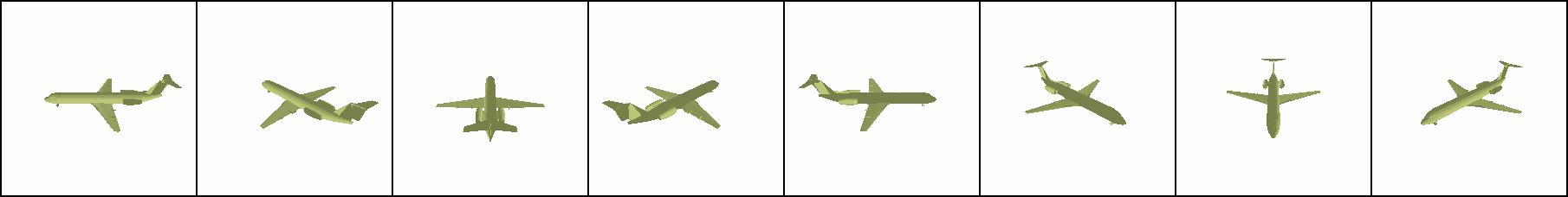
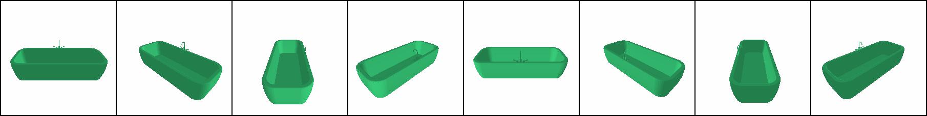
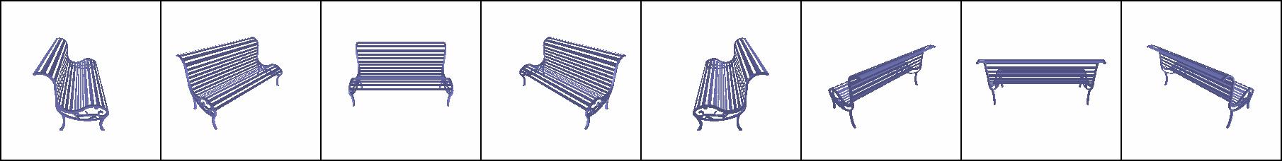
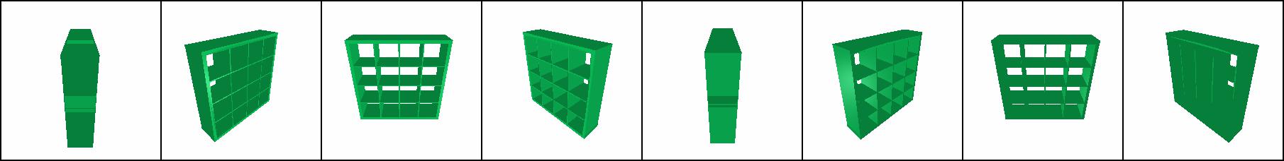
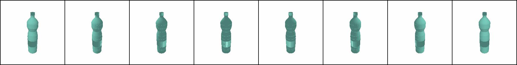
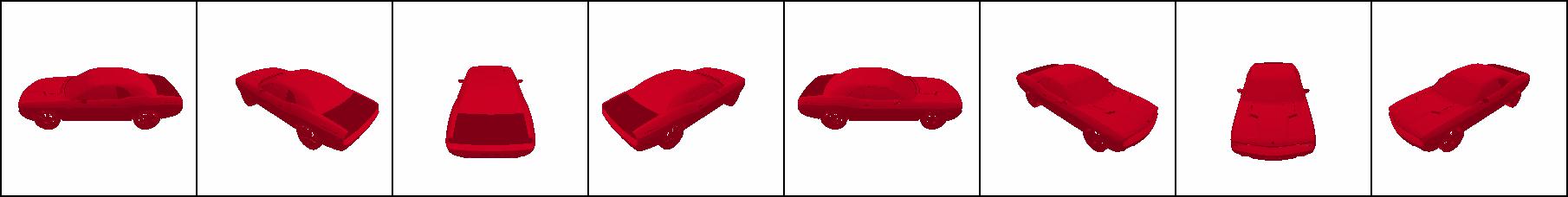
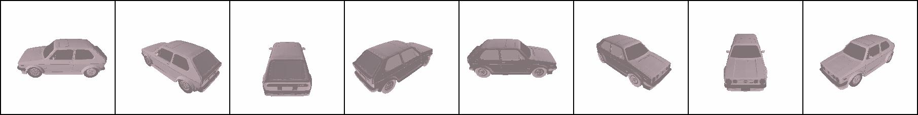
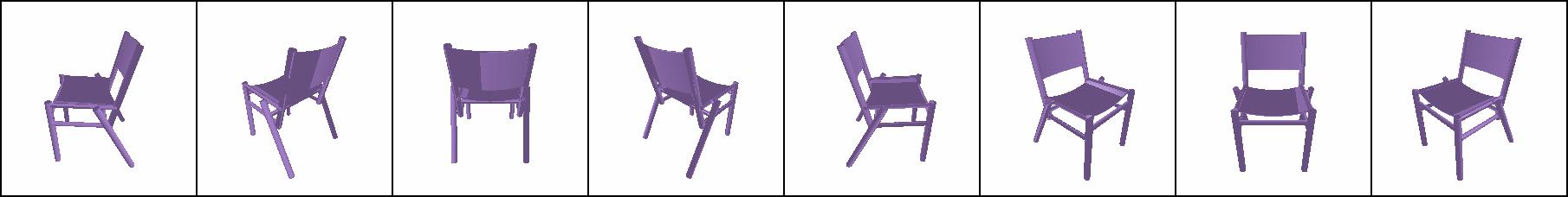
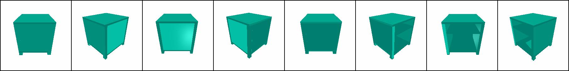
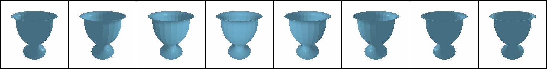
Figure 10: Training Data with Randomized Color and Lighting. We show examples of mesh renderings of ModelNet40 used in training our MVTN. The color of the object and the light’s direction are randomized during training for augmentation purposes and fixed in testing for stable performance. For this figure, eight circular views are shown for each 3D shape.

Figure 11: ShapeNet Core55. We show some examples of point cloud renderings of ShapeNet Core55 [10] used in training MVTN. Note how point cloud renderings offer more information about content hidden from the camera view-point (e.g. car wheels from the occluded side), which can be useful for recognition. For this figure, 12 spherical views are shown for each 3D shape.

Object Only
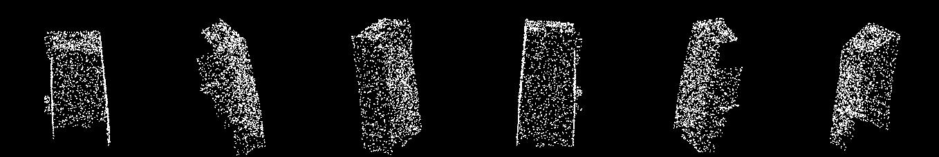
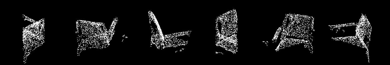
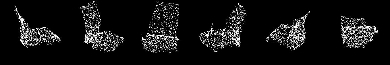
With Background
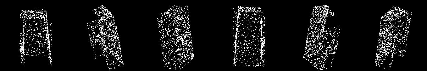
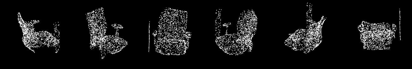
PB_T50_RS (Hardest)

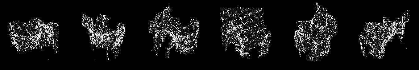
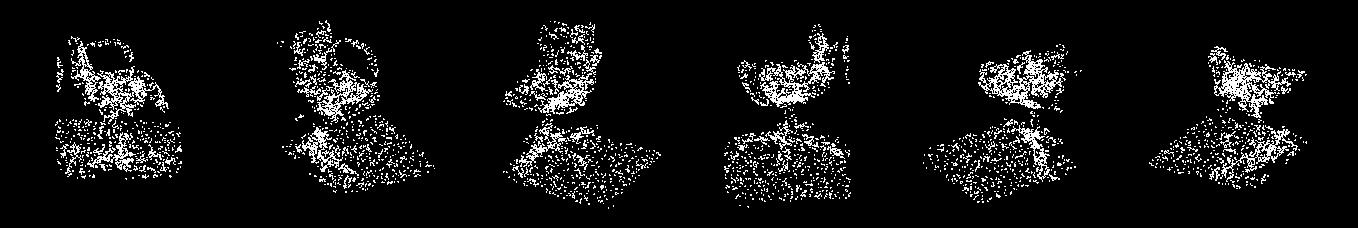
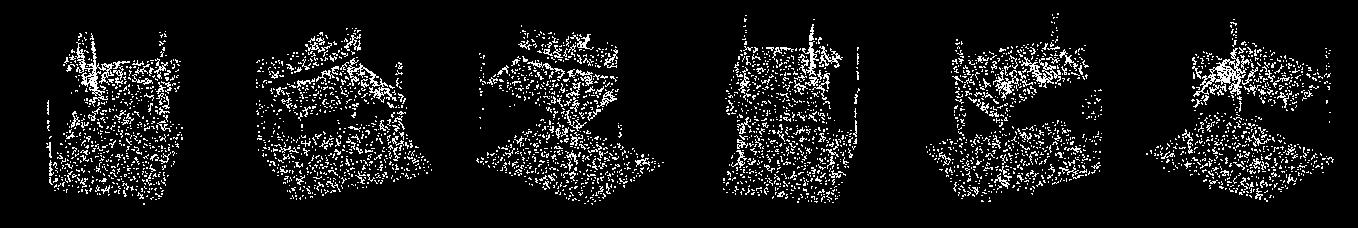
Figure 12: ScanObjectNN Variants. We show examples of point cloud renderings of different variants of the ScanObjectNN [78] point cloud dataset used to train MVTN. The variants are: object only, object with background, and the hardest perturbed variant (with rotation and translation). For this figure, six circular views are shown for each 3D shape.

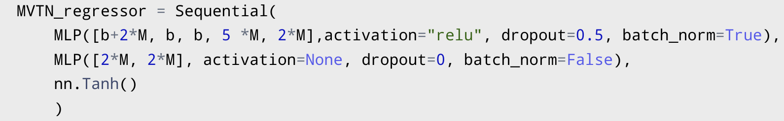
$b+2\times M$      $b$        $b$       $5\times M$       $2\times M$     $2\times M$

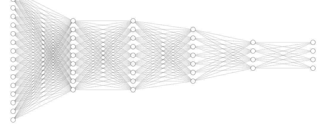
Figure 13: MVTN Network Architecture. We show a schematic and a code snippet for MVTN-spherical/MVTN-circular regression architectures used, where $b$ is the size of the point features extracted by the point encoder of MVTN and $M$ is the number of views learned. In most of our experiments, $b=40$, while the output is the azimuth and elevation angles for all the $M$ views used. The network is drawn using [54]

	1 view	2 views	4 views	6 views	8 views	10 views	12 views
(a)
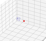
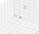
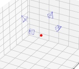
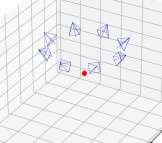
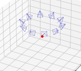
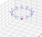
(b)
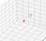
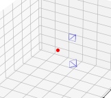
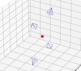
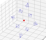
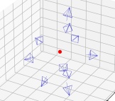
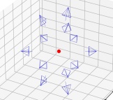
(c)

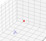
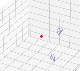
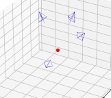
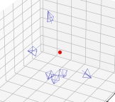
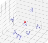
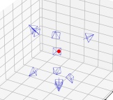
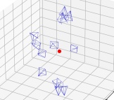
Figure 14: Views Configurations. We show some possible views configurations that can be used with a varying number of views. (a): circular, (b): spherical, (c): random

Appendix B Additional Results

B.1 Classification and Retrieval Benchmarks

We provide in Tables XIII,XIV, and XV comprehensive benchmarks of 3D classifications and 3D shape retrieval methods on ModelNet40 [85], ScanObjectNN [78], and ShapeNet Core55 [10, 74]. These tables include methods that use points as representations as well as other modalities like multi-view and volumetric representations. Our reported results of four runs are presented in each table as “max (avg $\pm$ std)”. Note in Table XIII how our MVTN improves the previous state-of-the-art in classification (ViewGCN [81]) when tested on the same setup. Our implementations (highlighted using $*$) slightly differ from the reported results in their original paper. This can be attributed to the specific differentiable renderer of Pytorch3D [72] that we are using, which might not have the same quality of the non-differentiable OpenGL renderings [83] used in their setups.

B.2 Rotation Robustness

A common practice in the literature in 3D shape classification is to test the robustness of models trained on the aligned dataset by injecting perturbations during test time [59]. We follow the same setup as [59] by introducing random rotations during test time around the Y-axis (gravity-axis). We also investigate the effect of varying rotation perturbations on the accuracy of circular MVCNN when $M=6$ and $M=12$. We note from Fig. 15 that using less views leads to higher sensitivity to rotations in general. Furthermore, we note that our MVTN helps in stabilizing the performance on increasing thresholds of rotation perturbations.

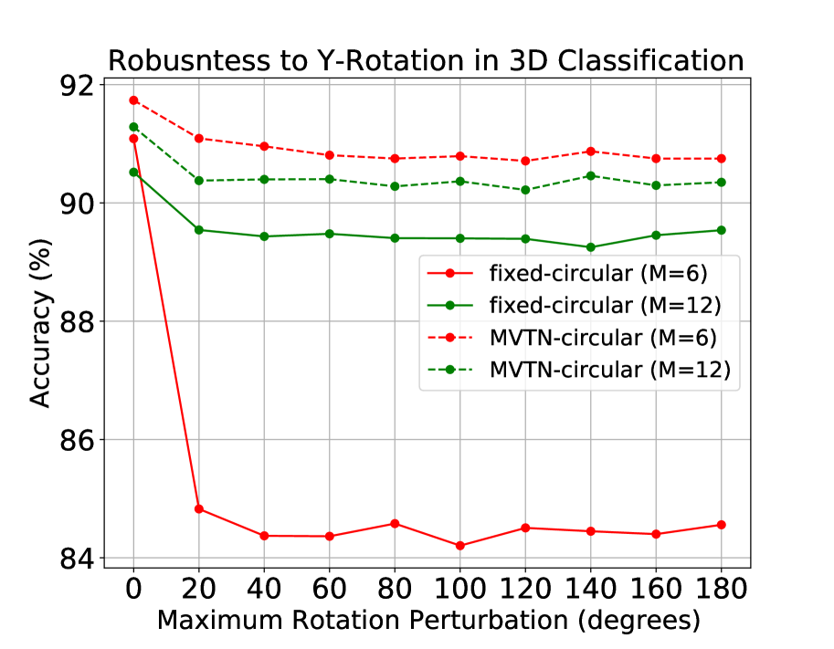
Figure 15: Robustness on a Varying Y-Rotation. We study the effect of varying the maximum rotation perturbation on the classification accuracies on ModelNet40. We compare the performance of circular MVCNN [75] to our circular-MVTN when it equips MVCNN when the number of views is 6 and 12. Note how MVTN stabilizes the drop in performance for larger Y-rotation perturbations, and the improvement is more significant for the smaller number of views $M$.

B.3 Occlusion Robustness

To quantify the occlusion effect due to the viewing angle of the 3D sensor in our setup of 3D classification, we simulate realistic occlusion by cropping the object from canonical directions. We train PointNet [68], DGCNN [80], and MVTN on the ModelNet40 point cloud dataset. Then, at test time, we crop a portion of the object (from 0% occlusion ratio to 75%) along the $\pm$X, $\pm$Y, and $\pm$Z directions independently. Fig. 17 shows examples of this occlusion effect with different occlusion ratios. We report the average test accuracy (on all the test set) of the six cropping directions for the baselines and MVTN in Fig. 16. Note how MVTN achieves high test accuracy even when large portions of the object are cropped. Interestingly, MVTN outperforms PointNet [68] by 13% in test accuracy when half of the object is occluded. This result is significant, given that PointNet is well-known for its robustness [68, 34].

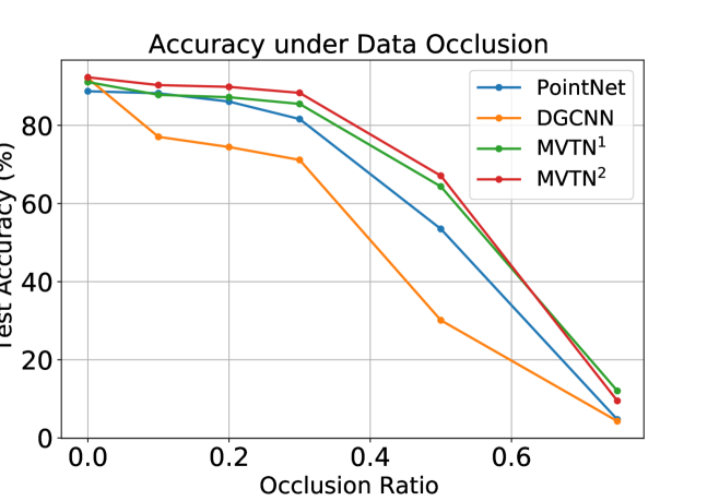
Figure 16: Occlusion Robustness of 3D Methods. We plot test accuracy vs. the Occlusion Ratio of the data to simulate the occlusion robustness of different 3D methods: PointNet [68], DGCNN [80], and MVTN. Our MVTN achieves close to 13% better than PointNet when half of the object is occluded. MVTN¹ refers to MVTN with MVCNN as the multi-view network while MVTN² refers to MVTN with View-GCN as the multi-view network.

		Classification Accuracy
Method	Data Type	(Per-Class)	(Overall)
SPH [48]	Voxels	68.2	-
LFD [13]	Voxels	75.5	-
3D ShapeNets [85]	Voxels	77.3	-
VoxNet [63]	Voxels	83.0	85.9
VRN [6]	Voxels	-	91.3
MVCNN-MS [70]	Voxels	-	91.4
FusionNet [39]	Voxels+MV	-	90.8
PointNet [68]	Points	86.2	89.2
PointNet++ [71]	Points	-	91.9
KD-Network [49]	Points	88.5	91.8
PointCNN [57]	Points	88.1	91.8
DGCNN [80]	Points	90.2	92.2
KPConv[77]	Points	-	92.9
PVNet[90]	Points	-	93.2
PTransformer[93]	Points	90.6	93.7
MVCNN [75]	12 Views	90.1	90.1
GVCNN [24]	12 Views	90.7	93.1
ViewGCN [81]	20 Views	96.5	97.6
ViewGCN [81]∗	12 views	90.7 (90.5 $\pm$ 0.2)	93.0 (92.8 $\pm$ 0.1)
ViewGCN [81]∗	20 views	91.3 (91.0 $\pm$ 0.2)	93.3 (93.1 $\pm$ 0.2)
MVTN (ours)∗	12 Views	92.0 (91.2 $\pm$ 0.6)	93.8 (93.4 $\pm$ 0.3)
MVTN (ours)∗	20 Views	92.2 (91.8 $\pm$ 0.3)	93.5 (93.1 $\pm$ 0.5)

TABLE XIII: 3D Shape Classification on ModelNet40. We compare MVTN against other methods in 3D classification on ModelNet40 [85]. ^∗ indicates results from our rendering setup (differentiable pipeline), while other multi-view results are reported from pre-rendered views. Bold denotes the best result in its setup. In brackets, we report the average and standard deviation of four runs

	Classification Overall Accuracy
Method	Object with Background	Object Only	PB_T50_RS (Hardest)
3DMFV [3]	68.2	73.8	63.0
PointNet [68]	73.3	79.2	68.0
SpiderCNN [87]	77.1	79.5	73.7
PointNet ++ [71]	82.3	84.3	77.9
PointCNN [57]	86.1	85.5	78.5
DGCNN [80]	82.8	86.2	78.1
SimpleView [28]	-	-	79.5
BGA-DGCNN [78]	-	-	79.7
BGA-PN++ [78]	-	-	80.2
ViewGCN ∗	91.9 (91.12 $\pm$ 0.5)	90.4 (89.7 $\pm$ 0.5)	80.5 (80.2 $\pm$ 0.4)
MVTN (ours)	92.6 (92.5 $\pm$ 0.2)	92.3 (91.7 $\pm$ 0.7)	82.8 (81.8 $\pm$ 0.7)

TABLE XIV: 3D Point Cloud Classification on ScanObjectNN. We compare the performance of MVTN in 3D point cloud classification on three different variants of ScanObjectNN [78]. The variants include object with background, object only, and the hardest variant. ^∗ indicates results from our rendering setup (differentiable pipeline), and we report the average and standard deviation of four runs in brackets.

		Shape Retrieval (mAP)
Method	Data Type	ModelNet40	ShapeNet Core
ZDFR [55]	Voxels	-	19.9
DLAN [25]	Voxels	-	66.3
SPH [48]	Voxels	33.3	-
LFD [13]	Voxels	40.9	-
3D ShapeNets [85]	Voxels	49.2	-
PVNet[90]	Points	89.5	-
MVCNN [75]	12 Views	80.2	73.5
GIFT [2]	20 Views	-	64.0
MVFusionNet [42]	12 Views	-	62.2
ReVGG [74]	20 Views	-	74.9
RotNet [46]	20 Views	-	77.2
ViewGCN [81]	20 Views	-	78.4
MLVCNN [43]	24 Views	92.2	-
MVTN (ours)	12 Views	92.9 (92.4 $\pm$ 0.6)	82.9 (82.4 $\pm$ 0.6)

TABLE XV: 3D Shape Retrieval. We benchmark the shape retrieval capability of MVTN on ModelNet40 [85] and ShapeNet Core55 [10, 74]. MVTN achieves the best retrieval performance among recent state-of-the-art methods on both datasets with only 12 views. In brackets, we report the average and standard deviation of four runs.

	Occlusion Ratio
Direction	0.1	0.2	0.3	0.5	0.75
+X
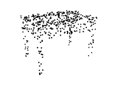
-X
+Z
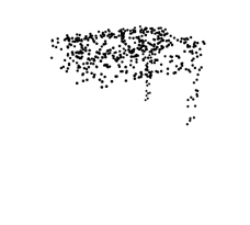
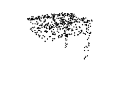
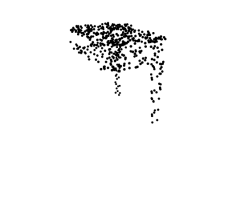
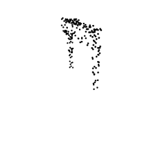
-Z
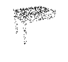
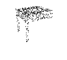
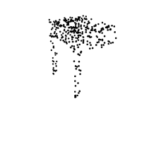
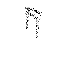
+Y
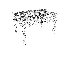
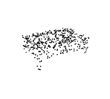
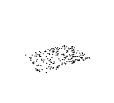
-Y

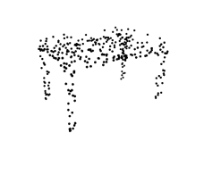
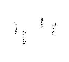
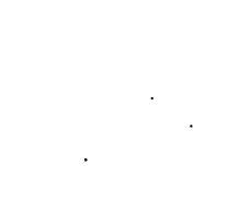
Figure 17: Occlusion of 3D Objects: We simulate realistic occlusion scenarios in 3D point clouds by cropping a percentage of the object along canonical directions. Here, we show an object occluded with different ratios and from different directions.

Appendix C Analysis and Insights

C.1 Ablation Study

This section introduces a comprehensive ablation study on the different components of MVTN, and their effect on test accuracy on the standard ModelNet40 [85].

MVTN Variants. We study the effect of the number of views $M$ on the performance of different MVTN variants (direct, circular, spherical). The experiments are repeated four times, and the average test accuracies with confidence intervals are shown in Fig. 18. The plots show how learned MVTN-spherical achieves consistently superior performance across a different number of views. Also, note that MVTN-direct suffers from over-fitting when the number of views is larger than four (i.e. it gets perfect training accuracy but deteriorates in test accuracy). This can be explained by observing that the predicted view-points tend to be similar to each other for MVTN-direct when the number of views is large. The similarity in views leads the multi-view network to memorize the training but to suffer in testing.

Backbone and Late Fusion. In the main manuscript (Table 6), we study MVTN with ViewGCN as the multi-view network. Here, we study the backbone effect on MVTN with MVCNN as the multi-view network and report all results in Table XVI. The study includes the backbone choice, the point encoder choice, and the type of aggregation method used to combine the multi-view network and the point encoder (late fusion vs. MVTN). Note that including more sophisticated backbones does not improve the accuracy, and using a late fusion mechanism is worse than our MVTN.

Light Direction Effect. We study the effect of light’s direction on the performance of multi-view networks. We note that picking a random light in training helps the network generalize to the test set. Please see Fig. 19 for the results on circular MVTN with MVCNN when comparing this strategy to fixed light from the top or from camera (relative). Note that we use relative light in test time to stabilize the performance.

Learning Distance to the Object. One possible ablation to the MVTN is to learn the distance to the object. This feature should allow the cameras to get closer to details that might be important to the classifier to understand the object properly. However, we observe that MVTN generally performs worse or does not improve with this setup, and hence, we refrain from learning it. In all of our main experiments, we fixed the distance to $2.2$ units, which is a good middle ground providing best accuracy. Please see Fig. 20 for the effect of picking a fixed distance in training spherical ViewGCN.

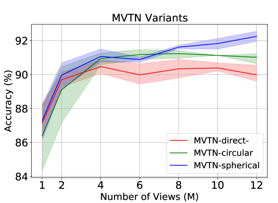
Figure 18: Variants of MVTN. We plot test accuracy vs. the number of views used in training different variants of our MVTN. Note how MVTN-spherical is generally more stable in achieving better performance on ModelNet40. 95% confidence interval is also plotted on each setup (repeated four times).

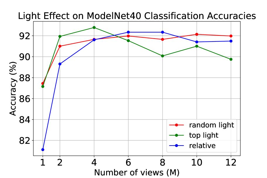
Figure 19: Light Direction Effect. We study the effect of light direction in the performance of the MVTN-circular. We note that randomizing the light direction in training reduce overfitting for larger number of views and leads to better generalization.

Effect of Distance

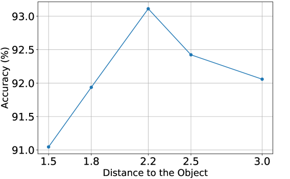
Figure 20: Effect of Distance to 3D Object. We study the effect of changing the distance on training a spherical ViewGCN. We show that the distance of 2.2 units to the center is in between far and close it and gives the best accuracy.

C.2 Transferability of MVTN View-Points

We hypothesize that the views learned by MVTN are transferable across multi-view classifiers. Looking at results in Fig. 22, 23, we believe MVTN picks the best views based on the actual shape and is less influenced by the multi-view network. This means that MVTN learns views that are more representative of the object, making it easier for any multi-view network to recognize it. As such, we ask the following: can we transfer the views MVTN learns under one setting to a different multi-view network?

To test our hypothesis, we take a 12-view MVTN-spherical module trained with MVCNN as a multi-view network and transfer the predicted views to a ViewGCN multi-view network. In this case, we freeze the MVTN module and only train ViewGCN on these learned but fixed views. ViewGCN with transferred MVTN views reaches $93.1\%$ accuracy in classification. It corresponds to a boost of $0.7\%$ from the $92.4\%$ of the original ViewGCN. Although this result is lower than fully trained MVTN($-0.3\%$), we observe a decent transferability between both multi-view architectures.

Views	Backbone		Point Encoder		Setup		Fusion		Results
number	ResNet18	ResNet50	PointNet[68]	DGCNN[80]	circular	spherical	late	MVTN	accuracy
6	✓	-	✓	-	✓	-	✓	-	90.48 %
6	✓	-	✓	-	✓	-	-	✓	91.13 %
6	✓	-	✓	-	-	✓	✓	-	89.51 %
6	✓	-	✓	-	-	✓	-	✓	91.94 %
6	✓	-	-	✓	✓	-	✓	-	87.80 %
6	✓	-	-	✓	✓	-	-	✓	91.49 %
6	✓	-	-	✓	-	✓	✓	-	89.82 %
6	✓	-	-	✓	-	✓	-	✓	91.29 %
6	-	✓	✓	-	✓	-	✓	-	89.10 %
6	-	✓	✓	-	✓	-	-	✓	90.40 %
6	-	✓	✓	-	-	✓	✓	-	89.22 %
6	-	✓	✓	-	-	✓	-	✓	90.76 %
6	-	✓	-	✓	✓	-	✓	-	89.99 %
6	-	✓	-	✓	✓	-	-	✓	89.91 %
6	-	✓	-	✓	-	✓	✓	-	89.95 %
6	-	✓	-	✓	-	✓	-	✓	90.43 %
12	✓	-	✓	-	✓	-	✓	-	87.35%
12	✓	-	✓	-	✓	-	-	✓	90.68%
12	✓	-	✓	-	-	✓	✓	-	88.41%
12	✓	-	✓	-	-	✓	-	✓	91.82
12	✓	-	-	✓	✓	-	✓	-	90.24%
12	✓	-	-	✓	✓	-	-	✓	90.28%
12	✓	-	-	✓	-	✓	✓	-	89.83%
12	✓	-	-	✓	-	✓	-	✓	91.98%
12	-	✓	✓	-	✓	-	✓	-	86.87%
12	-	✓	✓	-	✓	-	-	✓	88.86%
12	-	✓	✓	-	-	✓	✓	-	87.16%
12	-	✓	✓	-	-	✓	-	✓	88.41%
12	-	✓	-	✓	✓	-	✓	-	90.15%
12	-	✓	-	✓	✓	-	-	✓	88.37%
12	-	✓	-	✓	-	✓	✓	-	90.48%
12	-	✓	-	✓	-	✓	-	✓	89.63%

TABLE XVI: Ablation Study. We study the effect of ablating different components of MVTN on the test accuracy on ModelNet40. Namely, we observe that using more complex backbone CNNs (like ResNet50 [37]) or a more complex features extractor (like DGCNN [80]) does not increase the performance significantly compared to ResNet18 and PointNet [68] respectively. Furthermore, combining the shape features extractor with the MVCNN [75] in late fusion does not work as well as MVTN with the same architectures. All the reported results are using MVCNN [75] as multi-view network.

C.3 MVTN Predicted Views

We visualize the distribution of predicted views by MVTN for specific classes in Fig. 21. This is done to ensure that MVTN is learning per-instance views and regressing the same views for the entire class (collapse scenario). We can see that the MVTN distribution of the views varies from one class to another, and the views themselves on the same class have some variance from one instance to another. We also show specific examples for predicted views in Fig. 22, 23. Here, we show both the predicted camera view-points and the renderings from these cameras. Note how MVTN shifts every view to better show the discriminative details about the 3D object. To test that these views are per-instance, we average all the views predicted by our 4-view MVTN for every class and test the trained MVCNN on these fixed per-class views. In this setup, MVTN achieves 90.6% on ModelNet40, as compared to 91.0% for the per-instance views and 89% for the fixed views.

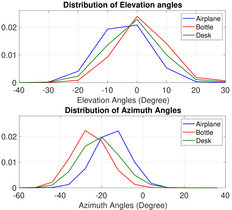
Figure 21: Visualizing MVTN learned Views. We visualize the distribution of azimuth and elevation angles predicted by the MVTN for three different classes. Note that MVTN learns inter-class variations (between different classes) and intra-class variations (on the same class).

circular:
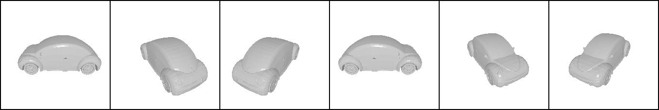
MVTN-circular:
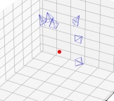
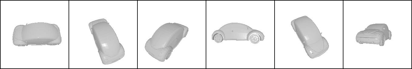
spherical:
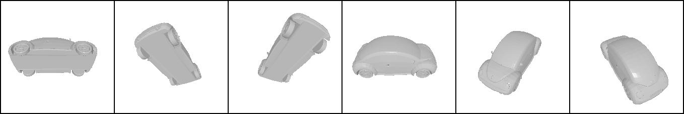
MVTN-spherical:
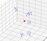
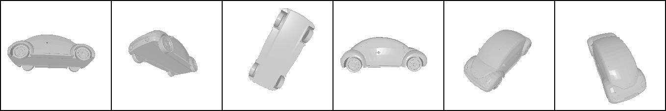
circular:
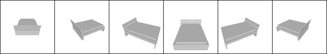
MVTN-circular:
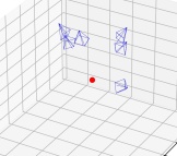
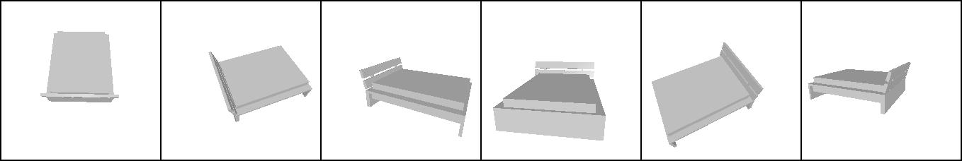
spherical:
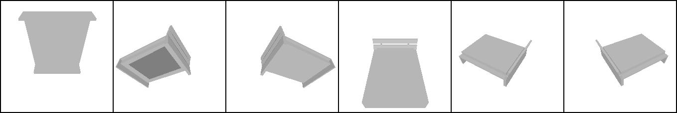
MVTN-spherical:

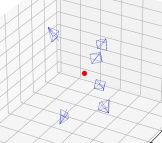
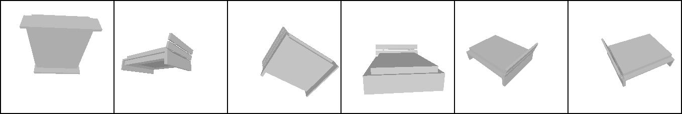
Figure 22: Qualitative Examples for MVTN predicted views (I): The view setups commonly followed in the multi-view literature are circular [75] or spherical [81, 46]. The red dot is the center of the object. MVTN-circular/MVTN-spherical are trained to predict the views as offsets to these common configurations. Note that MVTN adjust the original views to make the 3D object better represented by the multi-view images.

circular:
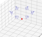
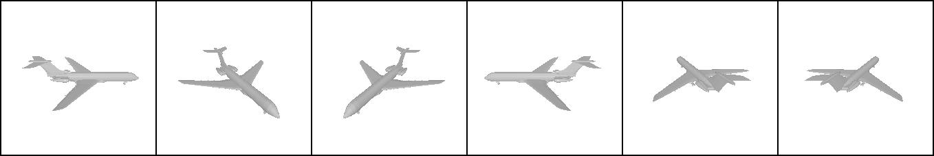
MVTN-circular:
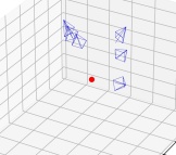
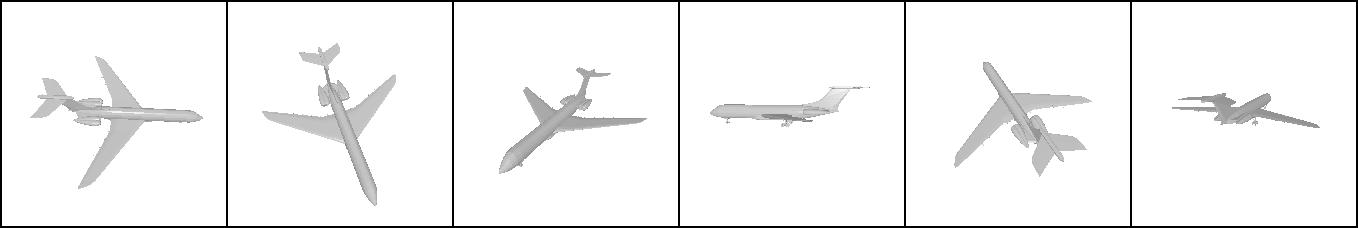
spherical:
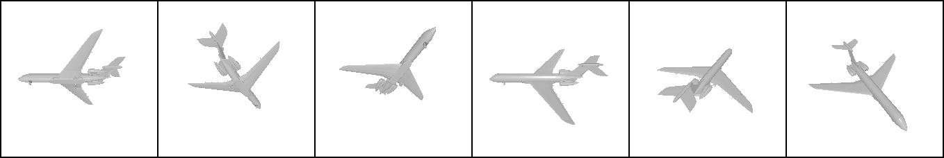
MVTN-spherical:
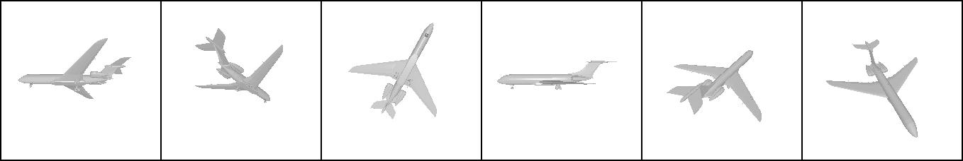
circular:
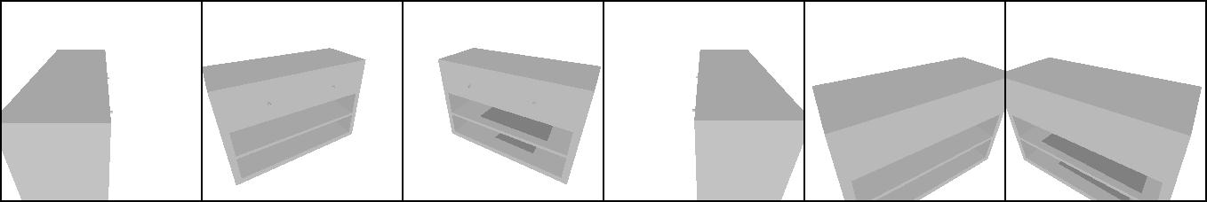
MVTN-circular:
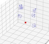
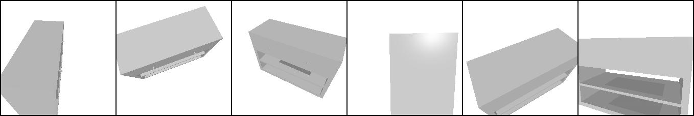
spherical:
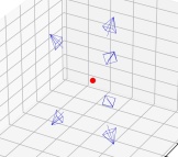
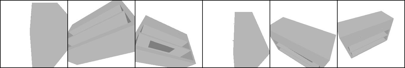
MVTN-spherical:

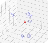
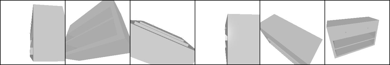
Figure 23: Qualitative Examples for MVTN predicted views (II): The view setups commonly followed in the multi-view literature are circular [75] or spherical [81, 46]. The red dot is the center of the object. MVTN-circular/MVTN-spherical are trained to predict the views as offsets to these common configurations. Note that MVTN adjust the original views to make the 3D object better represented by the multi-view images.

C.4 Shape Retrieval Examples

We show qualitative examples of our retrieval results using the MVTN-spherical with ViewGCN in Fig. 24. Note that the top ten retrieved objects for all these queries are positive (from the same classes of the queries).

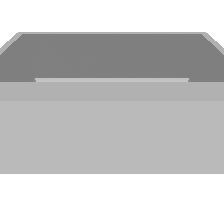
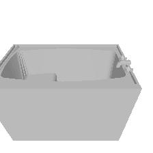
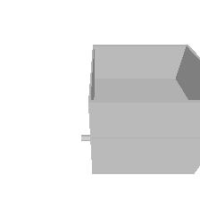
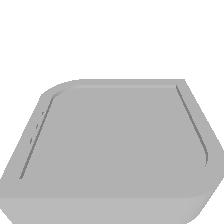
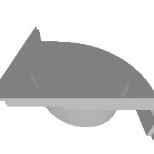
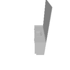
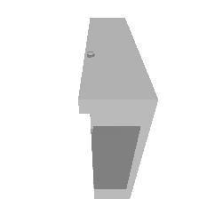
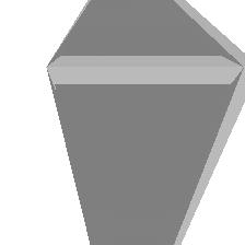
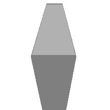
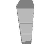
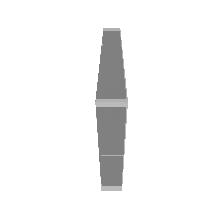
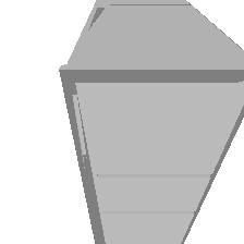
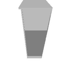
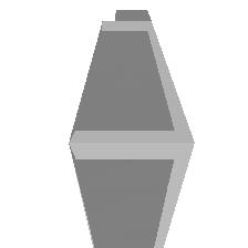
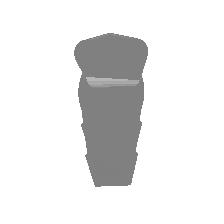
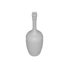
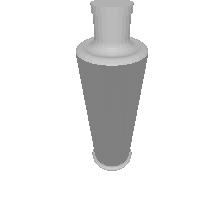
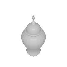
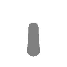
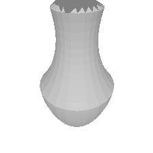
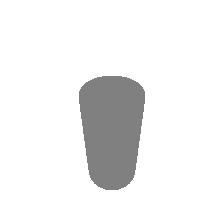
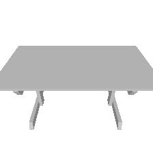
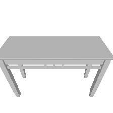
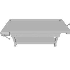
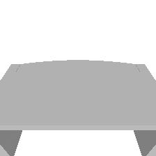
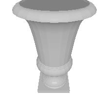
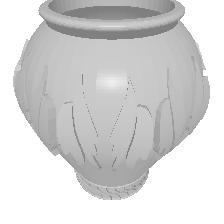
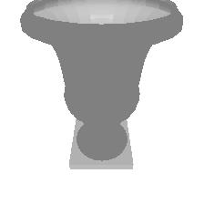
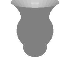
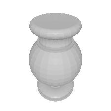
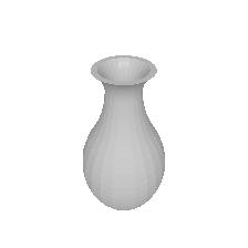
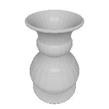
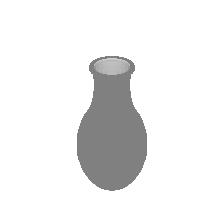
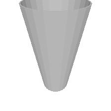
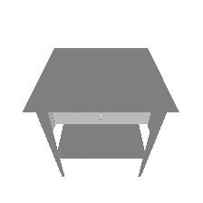
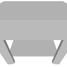
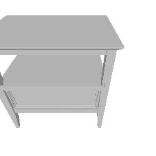
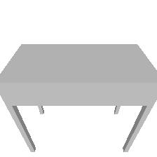
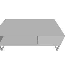
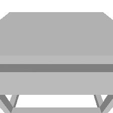
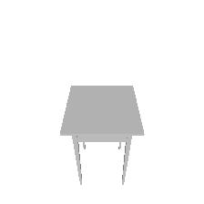
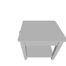
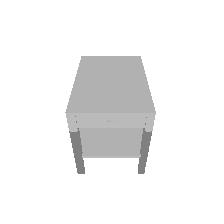
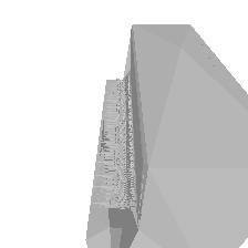
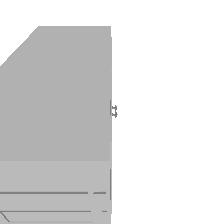
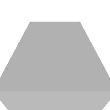
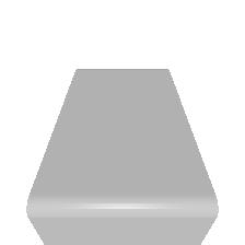
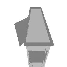
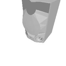
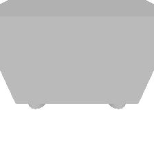
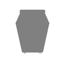
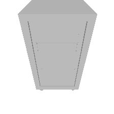
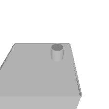
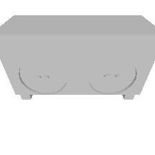
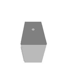
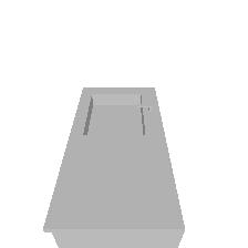
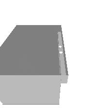
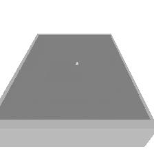
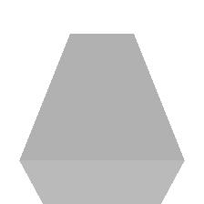
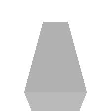
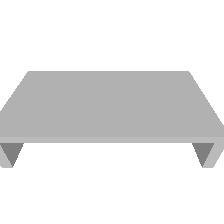
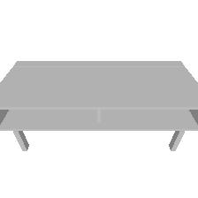
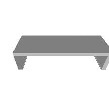
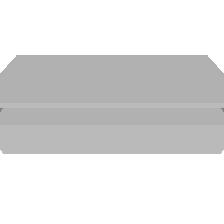
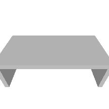
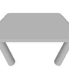
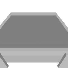
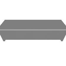
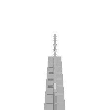
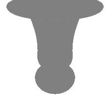
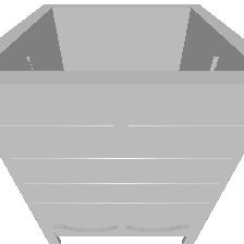
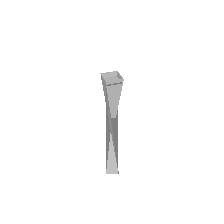
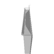
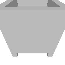
Figure 24: Qualitative Examples for Object Retrieval: (left): we show some query objects from the test set. (right): we show top ten retrieved objects by our MVTN from the training set.

References

- [1] Ceyhun Burak Akgül, Bülent Sankur, Yücel Yemez, and Francis Schmitt. 3d model retrieval using probability density-based shape descriptors. IEEE transactions on pattern analysis and machine intelligence, 31(6):1117–1133, 2009.
- [2] Song Bai, Xiang Bai, Zhichao Zhou, Zhaoxiang Zhang, and Longin Jan Latecki. Gift: A real-time and scalable 3d shape search engine. In Proceedings of the IEEE conference on computer vision and pattern recognition, pages 5023–5032, 2016.
- [3] Yizhak Ben-Shabat, Michael Lindenbaum, and Anath Fischer. 3dmfv: Three-dimensional point cloud classification in real-time using convolutional neural networks. IEEE Robotics and Automation Letters, 3(4):3145–3152, 2018.
- [4] Blender Online Community. Blender - a 3D modelling and rendering package. Blender Foundation, Blender Institute, Amsterdam, 2018.
- [5] Gary Bradski and Stephen Grossberg. Recognition of 3-d objects from multiple 2-d views by a self-organizing neural architecture. In From Statistics to Neural Networks, pages 349–375. Springer, 1994.
- [6] Andrew Brock, Theodore Lim, James M Ritchie, and Nick Weston. Generative and discriminative voxel modeling with convolutional neural networks. arXiv preprint arXiv:1608.04236, 2016.
- [7] Alexander M Bronstein, Michael M Bronstein, Leonidas J Guibas, and Maks Ovsjanikov. Shape google: Geometric words and expressions for invariant shape retrieval. ACM Transactions on Graphics (TOG), 30(1):1–20, 2011.
- [8] Nicholas Carlini and David Wagner. Towards evaluating the robustness of neural networks. In IEEE Symposium on Security and Privacy (SP), 2017.
- [9] Mathilde Caron, Hugo Touvron, Ishan Misra, Hervé Jégou, Julien Mairal, Piotr Bojanowski, and Armand Joulin. Emerging properties in self-supervised vision transformers. In Proceedings of the International Conference on Computer Vision (ICCV), 2021.
- [10] Angel X. Chang, Thomas Funkhouser, Leonidas Guibas, Pat Hanrahan, Qixing Huang, Zimo Li, Silvio Savarese, Manolis Savva, Shuran Song, Hao Su, Jianxiong Xiao, Li Yi, and Fisher Yu. ShapeNet: An Information-Rich 3D Model Repository. Technical Report arXiv:1512.03012 [cs.GR], Stanford University — Princeton University — Toyota Technological Institute at Chicago, 2015.
- [11] Siddhartha Chaudhuri and Vladlen Koltun. Data-driven suggestions for creativity support in 3d modeling. In ACM SIGGRAPH Asia 2010 papers, pages 1–10. 2010.
- [12] Ding-Yun Chen, Xiao-Pei Tian, Yu-Te Shen, and Ming Ouhyoung. On visual similarity based 3d model retrieval. In Computer graphics forum, volume 22, pages 223–232. Wiley Online Library, 2003.
- [13] Ding-Yun Chen, Xiao-Pei Tian, Yu-Te Shen, and Ming Ouhyoung. On visual similarity based 3d model retrieval. In Computer graphics forum, volume 22, pages 223–232. Wiley Online Library, 2003.
- [14] Liang-Chieh Chen, Yukun Zhu, George Papandreou, Florian Schroff, and Hartwig Adam. Encoder-decoder with atrous separable convolution for semantic image segmentation. In Proceedings of the European conference on computer vision (ECCV), pages 801–818, 2018.
- [15] Songle Chen, Lintao Zheng, Yan Zhang, Zhixin Sun, and Kai Xu. Veram: View-enhanced recurrent attention model for 3d shape classification. IEEE transactions on visualization and computer graphics, 25(12):3244–3257, 2018.
- [16] Wenzheng Chen, Huan Ling, Jun Gao, Edward Smith, Jaakko Lehtinen, Alec Jacobson, and Sanja Fidler. Learning to predict 3d objects with an interpolation-based differentiable renderer. In Advances in Neural Information Processing Systems, pages 9609–9619, 2019.
- [17] Christopher Choy, JunYoung Gwak, and Silvio Savarese. 4d spatio-temporal convnets: Minkowski convolutional neural networks. In Proceedings of the IEEE Conference on Computer Vision and Pattern Recognition, pages 3075–3084, 2019.
- [18] Taco Cohen and Max Welling. Group equivariant convolutional networks. In International conference on machine learning, pages 2990–2999, 2016.
- [19] Angela Dai and Matthias Nießner. 3dmv: Joint 3d-multi-view prediction for 3d semantic scene segmentation. In Proceedings of the European Conference on Computer Vision (ECCV), pages 452–468, 2018.
- [20] Markus Deserno. How to generate equidistributed points on the surface of a sphere. If Polymerforshung (Ed.), page 99, 2004.
- [21] Alexey Dosovitskiy, Lucas Beyer, Alexander Kolesnikov, Dirk Weissenborn, Xiaohua Zhai, Thomas Unterthiner, Mostafa Dehghani, Matthias Minderer, Georg Heigold, Sylvain Gelly, Jakob Uszkoreit, and Neil Houlsby. An image is worth 16x16 words: Transformers for image recognition at scale. ICLR, 2021.
- [22] Carlos Esteves, Yinshuang Xu, Christine Allen-Blanchette, and Kostas Daniilidis. Equivariant multi-view networks. In Proceedings of the IEEE International Conference on Computer Vision, pages 1568–1577, 2019.
- [23] Yutong Feng, Yifan Feng, Haoxuan You, Xibin Zhao, and Yue Gao. Meshnet: Mesh neural network for 3d shape representation. In Proceedings of the AAAI Conference on Artificial Intelligence, volume 33, pages 8279–8286, 2019.
- [24] Yifan Feng, Zizhao Zhang, Xibin Zhao, Rongrong Ji, and Yue Gao. Gvcnn: Group-view convolutional neural networks for 3d shape recognition. In Proceedings of the IEEE Conference on Computer Vision and Pattern Recognition, pages 264–272, 2018.
- [25] Takahiko Furuya and Ryutarou Ohbuchi. Deep aggregation of local 3d geometric features for 3d model retrieval. In BMVC, volume 7, page 8, 2016.
- [26] Yue Gao, Jinhui Tang, Richang Hong, Shuicheng Yan, Qionghai Dai, Naiyao Zhang, and Tat-Seng Chua. Camera constraint-free view-based 3-d object retrieval. IEEE Transactions on Image Processing, 21(4):2269–2281, 2011.
- [27] Michael Garland and Paul S Heckbert. Surface simplification using quadric error metrics. In Proceedings of the 24th annual conference on Computer graphics and interactive techniques, pages 209–216, 1997.
- [28] Ankit Goyal, Hei Law, Bowei Liu, Alejandro Newell, and Jia Deng. Revisiting point cloud shape classification with a simple and effective baseline. In ICML, 2021.
- [29] Benjamin Graham, Martin Engelcke, and Laurens Van Der Maaten. 3d semantic segmentation with submanifold sparse convolutional networks. In Proceedings of the IEEE conference on computer vision and pattern recognition, pages 9224–9232, 2018.
- [30] Ulf Grenander. Pattern analysis: lectures in pattern theory, volume I. Springer, 1978.
- [31] Abdullah Hamdi, Silvio Giancola, and Bernard Ghanem. Mvtn: Multi-view transformation network for 3d shape recognition. In Proceedings of the IEEE/CVF International Conference on Computer Vision (ICCV), pages 1–11, October 2021.
- [32] Abdullah Hamdi, Silvio Giancola, and Bernard Ghanem. Voint cloud: Multi-view point cloud representation for 3d understanding, 2021.
- [33] Abdullah Hamdi, Matthias Muller, and Bernard Ghanem. SADA: semantic adversarial diagnostic attacks for autonomous applications. In AAAI Conference on Artificial Intelligence, 2020.
- [34] Abdullah Hamdi, Sara Rojas, Ali Thabet, and Bernard Ghanem. Advpc: Transferable adversarial perturbations on 3d point clouds. In Computer Vision – ECCV 2020, pages 241–257, Cham, 2020. Springer International Publishing.
- [35] Rana Hanocka, Amir Hertz, Noa Fish, Raja Giryes, Shachar Fleishman, and Daniel Cohen-Or. Meshcnn: a network with an edge. ACM Transactions on Graphics (TOG), 38(4):1–12, 2019.
- [36] Kaiming He, Xinlei Chen, Saining Xie, Yanghao Li, Piotr Dollár, and Ross Girshick. Masked autoencoders are scalable vision learners, 2021.
- [37] Kaiming He, Xiangyu Zhang, Shaoqing Ren, and Jian Sun. Deep residual learning for image recognition. CoRR, abs/1512.03385, 2015.
- [38] Xinwei He, Yang Zhou, Zhichao Zhou, Song Bai, and Xiang Bai. Triplet-center loss for multi-view 3d object retrieval. In Proceedings of the IEEE Conference on Computer Vision and Pattern Recognition, pages 1945–1954, 2018.
- [39] Vishakh Hegde and Reza Zadeh. Fusionnet: 3d object classification using multiple data representations. arXiv preprint arXiv:1607.05695, 2016.
- [40] Max Jaderberg, Karen Simonyan, Andrew Zisserman, et al. Spatial transformer networks. In Advances in neural information processing systems, pages 2017–2025, 2015.
- [41] Maximilian Jaritz, Jiayuan Gu, and Hao Su. Multi-view pointnet for 3d scene understanding. In Proceedings of the IEEE International Conference on Computer Vision Workshops, pages 0–0, 2019.
- [42] Kui Jia, Jiehong Lin, Mingkui Tan, and Dacheng Tao. Deep multi-view learning using neuron-wise correlation-maximizing regularizers. IEEE Transactions on Image Processing, 28(10):5121–5134, 2019.
- [43] Jianwen Jiang, Di Bao, Ziqiang Chen, Xibin Zhao, and Yue Gao. Mlvcnn: Multi-loop-view convolutional neural network for 3d shape retrieval. In Proceedings of the AAAI Conference on Artificial Intelligence, volume 33, pages 8513–8520, 2019.
- [44] Danilo Jimenez Rezende, S. M. Ali Eslami, Shakir Mohamed, Peter Battaglia, Max Jaderberg, and Nicolas Heess. Unsupervised learning of 3d structure from images. In D. D. Lee, M. Sugiyama, U. V. Luxburg, I. Guyon, and R. Garnett, editors, Advances in Neural Information Processing Systems 29, pages 4996–5004. Curran Associates, Inc., 2016.
- [45] Evangelos Kalogerakis, Melinos Averkiou, Subhransu Maji, and Siddhartha Chaudhuri. 3d shape segmentation with projective convolutional networks. In proceedings of the IEEE conference on computer vision and pattern recognition, pages 3779–3788, 2017.
- [46] Asako Kanezaki, Yasuyuki Matsushita, and Yoshifumi Nishida. Rotationnet: Joint object categorization and pose estimation using multiviews from unsupervised viewpoints. In Proceedings of the IEEE Conference on Computer Vision and Pattern Recognition, pages 5010–5019, 2018.
- [47] Hiroharu Kato, Yoshitaka Ushiku, and Tatsuya Harada. Neural 3d mesh renderer. In Proceedings of the IEEE Conference on Computer Vision and Pattern Recognition (CVPR), pages 3907–3916, 2018.
- [48] Michael Kazhdan, Thomas Funkhouser, and Szymon Rusinkiewicz. Rotation invariant spherical harmonic representation of 3 d shape descriptors. In Symposium on geometry processing, volume 6, pages 156–164, 2003.
- [49] Roman Klokov and Victor Lempitsky. Escape from cells: Deep kd-networks for the recognition of 3d point cloud models. In Proceedings of the IEEE International Conference on Computer Vision, pages 863–872, 2017.
- [50] Tejas D Kulkarni, William F Whitney, Pushmeet Kohli, and Josh Tenenbaum. Deep convolutional inverse graphics network. In Advances in neural information processing systems (NIPS), pages 2539–2547, 2015.
- [51] Abhijit Kundu, Xiaoqi Yin, Alireza Fathi, David Ross, Brian Brewington, Thomas Funkhouser, and Caroline Pantofaru. Virtual multi-view fusion for 3d semantic segmentation. In European Conference on Computer Vision (ECCV), pages 518–535. Springer, 2020.
- [52] Loic Landrieu and Mohamed Boussaha. Point cloud oversegmentation with graph-structured deep metric learning. pages 7440–7449, 2019.
- [53] Loic Landrieu and Martin Simonovsky. Large-scale point cloud semantic segmentation with superpoint graphs. In Proceedings of the IEEE Conference on Computer Vision and Pattern Recognition (CVPR), pages 4558–4567, 2018.
- [54] Alex Lenail. Nn-svg, 2020.
- [55] Bo Li and Henry Johan. 3d model retrieval using hybrid features and class information. Multimedia tools and applications, 62(3):821–846, 2013.
- [56] Tzu-Mao Li, Miika Aittala, Frédo Durand, and Jaakko Lehtinen. Differentiable monte carlo ray tracing through edge sampling. In SIGGRAPH Asia 2018 Technical Papers, page 222. ACM, 2018.
- [57] Yangyan Li, Rui Bu, Mingchao Sun, Wei Wu, Xinhan Di, and Baoquan Chen. Pointcnn: Convolution on x-transformed points. In Advances in neural information processing systems (NIPS), pages 820–830, 2018.
- [58] Shichen Liu, Tianye Li, Weikai Chen, and Hao Li. Soft rasterizer: A differentiable renderer for image-based 3d reasoning. In Proceedings of the IEEE International Conference on Computer Vision, pages 7708–7717, 2019.
- [59] Yongcheng Liu, Bin Fan, Shiming Xiang, and Chunhong Pan. Relation-shape convolutional neural network for point cloud analysis. In Proceedings of the IEEE Conference on Computer Vision and Pattern Recognition, pages 8895–8904, 2019.
- [60] Zhijian Liu, Haotian Tang, Yujun Lin, and Song Han. Point-voxel cnn for efficient 3d deep learning. In Advances in Neural Information Processing Systems, pages 965–975, 2019.
- [61] Matthew M Loper and Michael J Black. Opendr: An approximate differentiable renderer. In European Conference on Computer Vision (ECCV), pages 154–169. Springer, 2014.
- [62] Ilya Loshchilov and Frank Hutter. Decoupled weight decay regularization. arXiv preprint arXiv:1711.05101, 2017.
- [63] Daniel Maturana and Sebastian Scherer. Voxnet: A 3d convolutional neural network for real-time object recognition. In 2015 IEEE/RSJ International Conference on Intelligent Robots and Systems (IROS), pages 922–928. IEEE, 2015.
- [64] Oscar Michel, Roi Bar-On, Richard Liu, Sagie Benaim, and Rana Hanocka. Text2mesh: Text-driven neural stylization for meshes. arXiv preprint arXiv:2112.03221, 2021.
- [65] Ben Mildenhall, Pratul P Srinivasan, Matthew Tancik, Jonathan T Barron, Ravi Ramamoorthi, and Ren Ng. Nerf: Representing scenes as neural radiance fields for view synthesis. In European conference on computer vision, pages 405–421. Springer, 2020.
- [66] Robert Osada, Thomas Funkhouser, Bernard Chazelle, and David Dobkin. Shape distributions. ACM Transactions on Graphics (TOG), 21(4):807–832, 2002.
- [67] Adam Paszke, Sam Gross, Soumith Chintala, Gregory Chanan, Edward Yang, Zachary DeVito, Zeming Lin, Alban Desmaison, Luca Antiga, and Adam Lerer. Automatic differentiation in pytorch. In NIPS-W, 2017.
- [68] Charles R Qi, Hao Su, Kaichun Mo, and Leonidas J Guibas. Pointnet: Deep learning on point sets for 3d classification and segmentation. In Proceedings of the IEEE Conference on Computer Vision and Pattern Recognition (CVPR), pages 652–660, 2017.
- [69] Charles R Qi, Hao Su, Matthias Nießner, Angela Dai, Mengyuan Yan, and Leonidas J Guibas. Volumetric and multi-view cnns for object classification on 3d data. In Proceedings of the IEEE conference on computer vision and pattern recognition, pages 5648–5656, 2016.
- [70] Charles R Qi, Hao Su, Matthias Nießner, Angela Dai, Mengyuan Yan, and Leonidas J Guibas. Volumetric and multi-view cnns for object classification on 3d data. In Proceedings of the IEEE conference on computer vision and pattern recognition, pages 5648–5656, 2016.
- [71] Charles Ruizhongtai Qi, Li Yi, Hao Su, and Leonidas J Guibas. Pointnet++: Deep hierarchical feature learning on point sets in a metric space. In Advances in neural information processing systems (NIPS), pages 5099–5108, 2017.
- [72] Nikhila Ravi, Jeremy Reizenstein, David Novotny, Taylor Gordon, Wan-Yen Lo, Justin Johnson, and Georgia Gkioxari. Accelerating 3d deep learning with pytorch3d. arXiv:2007.08501, 2020.
- [73] Olga Russakovsky, Jia Deng, Hao Su, Jonathan Krause, Sanjeev Satheesh, Sean Ma, Zhiheng Huang, Andrej Karpathy, Aditya Khosla, Michael S. Bernstein, Alexander C. Berg, and Fei-Fei Li. Imagenet large scale visual recognition challenge. CoRR, abs/1409.0575, 2014.
- [74] Konstantinos Sfikas, Theoharis Theoharis, and Ioannis Pratikakis. Exploiting the PANORAMA Representation for Convolutional Neural Network Classification and Retrieval. In Ioannis Pratikakis, Florent Dupont, and Maks Ovsjanikov, editors, Eurographics Workshop on 3D Object Retrieval, pages 1–7. The Eurographics Association, 2017.
- [75] Hang Su, Subhransu Maji, Evangelos Kalogerakis, and Erik Learned-Miller. Multi-view convolutional neural networks for 3d shape recognition. In Proceedings of the IEEE international conference on computer vision, pages 945–953, 2015.
- [76] Masashi Sugiyama. Dimensionality reduction of multimodal labeled data by local fisher discriminant analysis. Journal of machine learning research, 8(May):1027–1061, 2007.
- [77] Hugues Thomas, Charles R Qi, Jean-Emmanuel Deschaud, Beatriz Marcotegui, François Goulette, and Leonidas J Guibas. Kpconv: Flexible and deformable convolution for point clouds. In Proceedings of the IEEE/CVF International Conference on Computer Vision, pages 6411–6420, 2019.
- [78] Mikaela Angelina Uy, Quang-Hieu Pham, Binh-Son Hua, Duc Thanh Nguyen, and Sai-Kit Yeung. Revisiting point cloud classification: A new benchmark dataset and classification model on real-world data. In International Conference on Computer Vision (ICCV), 2019.
- [79] Weiyue Wang, Ronald Yu, Qiangui Huang, and Ulrich Neumann. Sgpn: Similarity group proposal network for 3d point cloud instance segmentation. In Proceedings of the IEEE Conference on Computer Vision and Pattern Recognition (CVPR), pages 2569–2578, 2018.
- [80] Yue Wang, Yongbin Sun, Ziwei Liu, Sanjay E. Sarma, Michael M. Bronstein, and Justin M. Solomon. Dynamic graph cnn for learning on point clouds. ACM Transactions on Graphics (TOG), 2019.
- [81] Xin Wei, Ruixuan Yu, and Jian Sun. View-gcn: View-based graph convolutional network for 3d shape analysis. In Proceedings of the IEEE/CVF Conference on Computer Vision and Pattern Recognition, pages 1850–1859, 2020.
- [82] Olivia Wiles, Georgia Gkioxari, Richard Szeliski, and Justin Johnson. Synsin: End-to-end view synthesis from a single image. In Proceedings of the IEEE/CVF Conference on Computer Vision and Pattern Recognition, pages 7467–7477, 2020.
- [83] Mason Woo, Jackie Neider, Tom Davis, and Dave Shreiner. OpenGL Programming Guide: The Official Guide to Learning OpenGL, Release 1. Addison-wesley, 1998.
- [84] Jiajun Wu, Joshua B Tenenbaum, and Pushmeet Kohli. Neural Scene De-rendering. In IEEE Conference on Computer Vision and Pattern Recognition (CVPR), 2017.
- [85] Zhirong Wu, S. Song, A. Khosla, Fisher Yu, Linguang Zhang, Xiaoou Tang, and J. Xiao. 3d shapenets: A deep representation for volumetric shapes. In 2015 IEEE Conference on Computer Vision and Pattern Recognition (CVPR), pages 1912–1920, 2015.
- [86] Zhirong Wu, Shuran Song, Aditya Khosla, Fisher Yu, Linguang Zhang, Xiaoou Tang, and Jianxiong Xiao. 3d shapenets: A deep representation for volumetric shapes. In Proceedings of the IEEE conference on computer vision and pattern recognition, pages 1912–1920, 2015.
- [87] Yifan Xu, Tianqi Fan, Mingye Xu, Long Zeng, and Yu Qiao. Spidercnn: Deep learning on point sets with parameterized convolutional filters. In Proceedings of the European Conference on Computer Vision (ECCV), pages 87–102, 2018.
- [88] Ze Yang and Liwei Wang. Learning relationships for multi-view 3d object recognition. In Proceedings of the IEEE International Conference on Computer Vision, pages 7505–7514, 2019.
- [89] Li Yi, Vladimir G Kim, Duygu Ceylan, I-Chao Shen, Mengyan Yan, Hao Su, Cewu Lu, Qixing Huang, Alla Sheffer, and Leonidas Guibas. A scalable active framework for region annotation in 3d shape collections. ACM Transactions on Graphics (ToG), 35(6):1–12, 2016.
- [90] Haoxuan You, Yifan Feng, Rongrong Ji, and Yue Gao. Pvnet: A joint convolutional network of point cloud and multi-view for 3d shape recognition. In Proceedings of the 26th ACM international conference on Multimedia, pages 1310–1318, 2018.
- [91] Tan Yu, Jingjing Meng, and Junsong Yuan. Multi-view harmonized bilinear network for 3d object recognition. In Proceedings of the IEEE Conference on Computer Vision and Pattern Recognition, pages 186–194, 2018.
- [92] Ye Yu and William AP Smith. Inverserendernet: Learning single image inverse rendering. arXiv preprint arXiv:1811.12328, 2018.
- [93] Hengshuang Zhao, Li Jiang, Jiaya Jia, Philip Torr, and Vladlen Koltun. Point transformer. arXiv preprint arXiv:2012.09164, 2020.