Crossingless sheaves and their classes in equivariant K-theory

Abstract.

We introduce crossingless sheaves in certain equivariant derived categories which are analogous to the Bezrukavnikov-Mirkovic exotic sheaves for two-block nilpotents. We calculate the classes of crossingless sheaves in equivariant K-theory of Cautis-Kamnitzer varieties.

1. Introduction

The exotic t-structure was defined by Bezrukavnikov and Mirkovic in [3] in order to study modular representation theory of Lie algebras. The exotic t-structure is defined using an action of the affine braid group on derived categories of varieties related to the Springer resolution defined by Bezrukavnikov and Riche in [4]. The irreducible objects in the heart of an exotic t-structure are called simple exotic sheaves.

More precisely, let $\bf k$ be an algebraically closed field of characteristic $p\gg 0$ and let $\mathfrak{g}$ be a reductive Lie algebra defined over $\bf k$. Let $\lambda$ be a regular integral weight and let $e$ be a nilpotent. Let ${\rm Mod}_{e}^{fg,\lambda}$ be the category of modules with genralized central character $(\lambda,e)$. Let $\mathcal{B}_{e,\bf k}$ be the Springer fiber corresponding to $e$. Then Theorem 5.3.1 of [2] states that

$$D^{b}(Coh_{\mathcal{B}_{e,\bf k}}(\widetilde{g}_{\bf k}))\simeq D^{b}({\rm Mod}_{e}^{fg,\lambda}).$$

It is also known that the tautological t-structure on the derived category of modules corresponds to the exotic t-structure on the derived category of coherent sheaves.

Exotic sheaves for two-block nilpotents were studied by Anno and Nandakumar in [1]. Let $\mathcal{D}_{n}^{\prime}$ be the derived category of coherent sheaves on a two-block Springer fibre (where the nilpotent is in type A and has two blocks of sizes $m+n$ and $n$). Anno and Nandakumar defined the objects $\Psi^{\prime}_{\alpha}\in D_{n}^{\prime}$ for any $(m,n)$-crossingless matching $\alpha$ and proved that these objects are the simple exotic sheaves for two-block nilpotents. Cautis-Kamnitzer varieties $Y_{k}$ which contain Springer fibers and Slodowy slices were introduced in [5] (see Definition 3.1). The equivariant K-theory of $Y_{k}$ is a free $\mathbb{C}[q,q^{-1}]$-module on $2^{k}$ generators (See Proposition 3.3). Classes of $\Psi^{\prime}_{\alpha}$ in K-theory of Cautis-Kamnitzer varieties were computed in [7] and subsequently applied to the calculation of dimensions of modular representations of $\mathfrak{sl}_{n}$ with a two-block central character.

Cautis and Kamnitzer studied categorification of Reshetikhin-Turaev invariants of linear tangles in [5]. In the course of their study they defined functors $\Psi(\alpha)$ for linear tangles $\alpha$. We complete their representation to a representation of affine tangles so that we have functors $\Psi(\alpha)$ for any affine tangle $\alpha$. Using these functors, we define an analogous concept to Anno-Nandakumar’s exotic sheaves for a two-block nilpotent in certain equivariant derived category. We call the objects we defined crossingless sheaves (see Definition 3.11). We compute the classes of crossingless sheaves in equivaraint K-theory of Cautis-Kamnitzer varieties (see Theorem 3.23, which is our main theorem).

This paper introduces techniques which can be used for defining representations of affine tangles on equivariant derived category of Cautis-Kamnitzer varieties with respect to the ${\mathbb{C}}^{*}$ in the centralizer of the two-block nilpotent and calculating characters of modular representations with central character equal to a two-block nilpotent (note that dimension formulas for these modular representations have been computed in [7]). These goals will be achieved in subsequent publications by the author.

Acknowledgements

I thank Vinoth Nandakumar for sharing his ideas and for many useful conversations. I also thank Joel Kamnitzer for useful correspondence and Roman Travkin for helpful conversations.

2. Preliminaries

2.1. Affine tangles

The combinatorics of affine tangles will be necessary for what follows; we recall the definitions here (see Section 3 of [1] for more details).

Definition 2.1.

If $q\equiv r\pmod{2}$, a $(q,r)$ affine tangle is an embedding (up to isotopy) of $\frac{q+r}{2}$ arcs and a finite number of circles into the region $\{(x,y)\in\mathbb{C}\times\mathbb{R}|1\leq|x|\leq 2\}$, such that the end-points of the arcs are $(1,0),(\zeta_{q},0),\cdots,(\zeta_{q}^{q-1},0),(2,0),(2\zeta_{r},0),\cdots,(2\zeta_{r}^{r-1},0)$ in some order; here $\zeta_{k}=e^{\frac{2\pi i}{k}}$.

Figure 1 illustrates the composition of affine tangles.

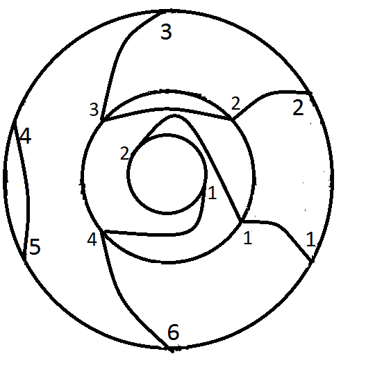
Figure 1.

Definition 2.2.

If $q\equiv r\pmod{2}$, a framed $(q,r)$ affine tangle is an embedding (up to isotopy) of $\frac{q+r}{2}$ “rectangular arcs” and a finite number of circles into the region $\{(x,y)\in\mathbb{C}\times\mathbb{R}|1\leq|x|\leq 2\}$. Here a “rectangular arc” is an injective map from $[0,1]\times[0,1]$ to $\{(x,y)\in\mathbb{C}\times\mathbb{R}|1\leq|x|\leq 2\}$ where the segments $[0,1]\times 0$ and $[0,1]\times 1$ are mapped to the segments $[x]\times[0,1]$ where $x=\zeta_{p}^{i}$ or $x=2\zeta_{q}^{j}$.

Remark 2.3.

Framed tangles are necessary for the validity of the Reidemeister I move in the functorial tangle categorification statement from Proposition 3.9. Below we will often abbreviate “$(q,r)$-affine tangle” to “$(q,r)$-tangle”. In [1], we used $\;\widehat{}\;$ notation to denote framed tangles; we omit that here. Note that given a $(q,r)$ framed affine tangle $\alpha$, and a $(r,s)$ framed affine tangle $\beta$, we can compose them using scaling and concatenation to obtain a $(q,s)$ affine tangle $\beta\circ\alpha$. This composition is associative up to isotopy.

Definition 2.4.

Given $1\leq i\leq n$, define the following affine tangles:

• Let $g_{n}^{i}$ denote the $(n-2,n)$ tangle with an arc connecting $(2\zeta_{n}^{i},0)$ to $(2\zeta_{n}^{i+1},0)$.

• Let $f_{n}^{i}$ denote the $(n,n-2)$ tangle with an arc connecting $(\zeta_{n}^{i},0)$ and $(\zeta_{n}^{i+1},0)$.

• Let $t_{n}^{i}(1)$ (respectively, $t^{i}_{n}(2)$) denote the $(n,n)$ tangle in which a strand connecting $(\zeta_{n}^{i},0)$ to $(2\zeta_{n}^{i+1},0)$ passes above (respectively, beneath) a strand connecting $(\zeta_{n}^{i+1},0)$ to $(2\zeta_{n}^{i},0)$.

• Let $r_{n}$ denote the $(n,n)$ tangle connecting $(\zeta_{n}^{j},0)$ to $(2\zeta_{n}^{j-1},0)$ for each $1\leq j\leq n$ (clockwise rotation of all strands).

• Let $s_{n}^{i}$ denote the $(n,n)$-tangle with a strand connecting $(\zeta_{j},0)$ to $(2\zeta_{j},0)$ for each $j$, and a strand connecting $(\zeta_{i},0)$ to $(2\zeta_{i},0)$ passing clockwise around the circle, beneath all the other strands.

We also introduce new generators $w_{n}^{i}(1)$ and $w_{n}^{i}(2)$, which correspond to positive and negative twists of framing of the $i$-th strand of an $(n,n)$ identity tangle.

The below figures depict some of these elementary tangles. Here the label $i$ in the inner (resp. outer) circle denotes the point $(\zeta^{i},0)$ (resp. $(2\zeta^{i},0)$).

These are called “elementary” tangles because any framed tangle can be expressed as (or rather, is isotopic to) a product of the tangles $g_{n}^{i},,f_{n}^{i},t_{n}^{i}(1),t_{n}^{i}(2),w_{n}^{i}(1),w_{n}^{i}(2)$ and $r_{n}$. Alternatively, this statement is true if we replace $r_{n}$ by $s_{n}^{n}$ (to see this, one uses the fact that $r_{n}=s_{n}^{n}\circ t_{n}^{n-1}(2)\circ\cdots\circ t_{n}^{1}(2)$).

Definition 2.5.

A $(q,r)$-tangle is a“linear tangle” if it can be expressed in terms of the generators $g_{n}^{i},f_{n}^{i},t_{n}^{i}(1),t_{n}^{i}(2),w_{n}^{i}(1),w_{n}^{i}(2)$ (i.e. without using $r_{n}$).

The above definition is motivated that the fact any such tangle can be represented with endpoints on a line segment (as opposed to an annulus); see Section 4 of [5] for a pictorial depiction.

Below is the list of relations which the generators $g_{n}^{i},f_{n}^{i},t_{n}^{i}(1),t_{n}^{i}(2),w_{n}^{i}(1),w_{n}^{i}(2),r_{n}$ satisfy. Note that $r^{\prime}_{n}$ is the inverse of $r_{n}$.

1. ${f}_{n}^{i}\circ{g}_{n}^{i+1}=id={f}_{n}^{i+1}\circ{g}_{n}^{i}$

2. (Reidemeister 1) ${f}_{n}^{i}\circ{t}_{n}^{i\pm 1}(l)\circ{g}_{n}^{i}={w}_{n}^{i}(l)$

3. ${t}_{n}^{i}(2)\circ{t}_{n}^{i}(1)=id={t}_{n}^{i}(1)\circ{t}_{n}^{i}(2)$

4. ${t}_{n}^{i}(l)\circ{t}_{n}^{i+1}(l)\circ{t}_{n}^{i}(l)={t}_{n}^{i+1}(l)\circ{t}_{n}^{i}(l)\circ{t}_{n}^{i+1}(l)$

5. ${g}_{n+2}^{i+k}\circ{g}_{n}^{i}={g}_{n+2}^{i}\circ{g}_{n}^{i+k-2}$

6. ${f}_{n}^{i+k-2}\circ{f}_{n+2}^{i}={f}_{n}^{i}\circ{f}_{n+2}^{i+k}$

7. ${g}_{n}^{i+k-2}\circ{f}_{n}^{i}={f}_{n+2}^{i}\circ{g}_{n+2}^{i+k},\quad{g}_{n}^{i}\circ{f}_{n}^{i+k-2}={f}_{n+2}^{i+k}\circ{g}_{n+2}^{i}$

8. ${g}_{n}^{i}\circ{t}_{n-2}^{i+k-2}(l)={t}_{n}^{i+k}(l)\circ{g}_{n}^{i},\quad{g}_{n}^{i+k}\circ{t}_{n-2}^{i}(l)={t}_{n}^{i}(l)\circ{g}_{n}^{i+k}$

9. ${f}_{n}^{i}\circ{t}_{n}^{i+k}(l)={t}_{n-2}^{i+k-2}(l)\circ{f}_{n}^{i},\quad{f}_{n}^{i+k}\circ{t}_{n}^{i}(l)={t}_{n-2}^{i}(l)\circ{f}_{n}^{i+k}$

10. ${t}_{n}^{i}(l)\circ{t}_{n}^{i+k}(m)={t}_{n}^{i+k}(m)\circ{t}_{n}^{i}(l)$

11. ${t}_{n}^{i}(1)\circ{g}_{n}^{i+1}={t}_{n}^{i+1}(2)\circ{g}_{n}^{i},\quad{t}_{n}^{i}(2)\circ{g}_{n}^{i+1}={t}_{n}^{i+1}(1)\circ{g}_{n}^{i}$

12. ${r}_{n}\circ{r}_{n}^{\prime}=id={r}_{n}^{\prime}\circ{r}_{n}$

13. ${r}_{n-2}^{\prime}\circ{f}_{n}^{i}\circ{r}_{n}={f}_{n}^{i+1},\ i=1,\ldots,n-2;\quad{f}_{n}^{n-1}\circ({r}_{n})^{2}={f}_{n}^{1}$

14. ${r}_{n}^{\prime}\circ{g}_{n}^{i}\circ{r}_{n-2}={g}_{n}^{i+1},\ i=1,\ldots,n-2;\quad({r}_{n}^{\prime})^{2}\circ{g}_{n}^{n-1}={g}_{n}^{1}$

15. ${r}_{n}^{\prime}\circ{t}_{n}^{i}(l)\circ{r}_{n}={t}_{n}^{i+1}(l);\quad({r}_{n}^{\prime})^{2}\circ{t}_{n}^{n-1}(l)\circ({r}_{n})^{2}={t}_{n}^{1}(l)$

    We have the following additional relations for twists:

16. ${w}_{n}^{i}(1)\circ{w}_{n}^{i}(2)=id,\quad{w}_{n}^{i}(l)\circ{w}_{n}^{j}(k)={w}_{n}^{j}(k)\circ{w}_{n}^{i}(l),\ i\neq j$

17. $\hat{w}_{n}^{i}(k)\circ{g}_{n}^{i}={w}_{n}^{i+1}(k)\circ{g}_{n}^{i},\quad{w}_{n}^{i}(k)\circ{g}_{n}^{j}={g}_{n}^{j}\circ{w}_{n}^{i+1\pm 1}(k),\ i\neq j,j+1$

18. ${f}_{n}^{i}\circ{w}_{n}^{i}(k)={f}_{n}^{i}\circ{w}_{n}^{i+1}(k),\quad{w}_{n}^{i}(k)\circ{f}_{n}^{j}={f}_{n}^{j}\circ{w}_{n}^{i-1\pm 1}(k),\ i\neq j,j+1$

19. ${w}_{n}^{i}(k)\circ{t}_{n}^{i}(l)={w}_{n}^{i+1}(k)\circ{t}_{n}^{i}(l),\quad{w}_{n}^{i}(k)\circ{t}_{n}^{j}(l)={t}_{n}^{j}(l)\circ{w}_{n}^{i}(k),\ i\neq j,j+1$

20. ${t}_{n}^{i}\circ{w}_{n}^{i}(k)={f}_{n}^{i}\circ{w}_{n}^{i+1}(k),\quad{w}_{n}^{i}(k)\circ{f}_{n}^{j}={t}_{n}^{j}\circ{w}_{n}^{i}(k),\ i\neq j,j+1$

21. ${w}_{n}^{i}(k)\circ{r}_{n}={r}_{n}\circ{w}_{n}^{i-1}(k),\quad{w}_{n}^{i}(k)\circ{r}^{\prime}_{n}={r}^{\prime}_{n}\circ{w}_{n}^{i+1}(k)$

2.2. Exotic t-structures for two-block nilpotents

In this section we summarize the results of [1] for motivational purposes. Let $\mathfrak{g}=\mathfrak{sl}_{m+2n}$, and $\mathcal{B}$ be the flag variety. Let $e\in\mathfrak{g}^{*}$ be a nilpotent linear functional with Jordan type $(m+n,n)$, and $\lambda\in\mathfrak{h}^{*}//W$ be a regular Harish-Chandra character.

Let $S_{m,n}\subset\mathfrak{g}$ be the corresponding Mirkovic-Vybornov transverse slice (see [8] for a definition, and see below for an explicit matrix realization). Let $U_{m+n,n}\subset\tilde{\mathfrak{g}}=T^{*}\mathcal{B}$ be its preimage under the Grothendieck-Springer resolution map.

$$S_{m,n} =\{\left(\begin{array}[]{ccccccccc}&1&&&&&&&\\ &&&\ddots&&&&&\\ &&&&1&&&&\\ a_{1}&a_{2}&&\cdots&a_{m+n}&b_{1}&b_{2}&\cdots&b_{n}\\ &&&&&&1&&\\ &&&&&&&\ddots&\\ &&&&&&&&1\\ c_{1}&\cdots&c_{n}\;0&\cdots&0&d_{1}&d_{2}&\cdots&d_{n}\end{array}\right)\}$$

Definition 2.6.

Let $\langle\cdot,\cdot\rangle$ denote the Killing form.

$$S^{*}_{m,n} =\{x\in\mathfrak{g}\;|\;\langle x,z-e\rangle=0\;\forall\;z\in S_{m,n}\}$$

$$\textbf{U}_{\hat{e}}\mathfrak{g} =\textbf{U}\mathfrak{g}/\langle x^{p}-x^{[p]}-\langle e,x\rangle^{p}\;|\;x\in S^{*}_{m,n}\rangle$$

Denote by $\text{Mod}_{\hat{e},\lambda}^{fg}(\textbf{U}\mathfrak{g})$ the subcategory of $\text{Mod}_{e,\lambda}^{fg}(\textbf{U}\mathfrak{g})$ consisting of those modules which are defined over the quotient $\textbf{U}_{\hat{e}}\mathfrak{g}$.

[BMR] localization theory gives the equivalence in the below Proposition; see Section 5.1 of [1] for more details. Under this equivalence, the tautological t-structure on the LHS is mapped to the exotic t-structure on the RHS. We refer to the images of the irreducible objects in the LHS as simple exotic sheaves.

Proposition 2.7.

$$\mathcal{C}_{m,n}:=D^{b}\text{Mod}^{\text{fg}}_{\hat{e},\lambda}(U\mathfrak{g})\simeq D^{b}\text{Coh}_{\mathcal{B}_{e}}(U_{e})$$

Proposition 2.8.

Let $\alpha$ be an $(m+2p,m+2q)$-tangle. Then we have a functor $\Psi^{\prime}(\alpha):\mathcal{C}_{m,p}\rightarrow\mathcal{C}_{m,q}$; this collection of functors satisfy the functorial tangle relations $\Psi^{\prime}(\alpha)\circ\Psi^{\prime}(\beta)\simeq\Psi^{\prime}(\alpha\circ\beta)$.

These are defined by Fourier-Mukai transforms on the categories of coherent sheaves; see Section $4$ of [1] for more details of the proof. These functors can be used to describe the simple exotic sheaves as follows.

Definition 2.9.

Let $\text{Cross}(m,n)$ be the set of all matchings on an annulus with $m$ unlabelled points on the inner circle, $m+2n$ labelled points on the outer circle (with labels $1,\cdots,m+2n$), such that there are no crossings or loops, and each point on the inner circle is connected to a point on the outer circle.

Example 2.10.

See Figure 2 for an example of an element $\alpha\in\text{Cross}(2,2)$.

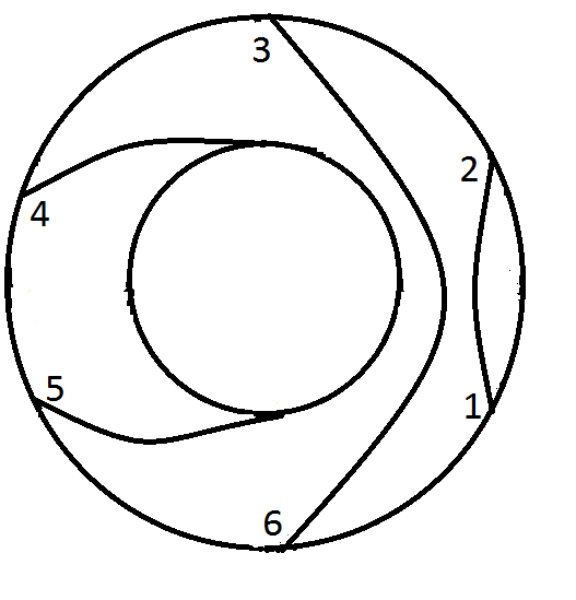
Figure 2.

Definition 2.11.

Each $\alpha\in\text{Cross}(m,n)$ can be viewed as a framed tangle, with the trivial framing. Thus using Proposition 2.8 we have a functor $\Psi^{\prime}(\alpha):\mathcal{C}_{m,0}\rightarrow\mathcal{C}_{m,n}$. Since $\mathcal{B}_{e}$ is a point when $n=0$, it follows that $\mathcal{C}_{m,0}\simeq D^{b}(\text{Vect})$.Given $\alpha\in\text{Cross}(m,n)$, let $\Psi^{\prime}_{\alpha}=\Psi^{\prime}(\alpha)(\textbf{k})$.

Theorem 2.12.

The objects $\{\Psi^{\prime}_{\alpha}\;|\;\alpha\in\text{Cross}(m,n)\}$ are the simple exotic sheaves.

See Section 5.3 of [1] for a proof of the above theorem.

3. Coherent sheaves on Cautis-Kamnitzer varieties and the main theorem

We will need Cautis-Kamnitzer’s framework for much of what follows. The Cautis-Kamnitzer varieties $Y_{k}$ are constructed as follows (see Section 2.1 of [5] for more details):

Definition 3.1.

Consider a $2k$-dimensional vector space $V_{k}$ over $\mathbb{C}$ with basis $e_{1},\ldots,e_{k},f_{1},\ldots,f_{k}$ and a nilpotent $z$ such that $ze_{i+1}=e_{i}$, $zf_{i+1}=f_{i}$ for $i\geq 1$, and $ze_{1}=zf_{1}=0$. Let $L_{0}=0$. Then:

$$Y_{k}=\{(L_{1}\subset\cdots\subset L_{k}\subset V_{k})\;|\;\text{ dim}(L_{i})=i,\ zL_{i}\subset L_{i-1}\}$$

Let $\mathbb{C}^{*}$ act on $V_{k}$ by $t\cdot e_{i}=t^{-2i}e_{i}$ and $t\cdot f_{i}=t^{-2i}f_{i}$. This $\mathbb{C}^{*}$-action induces a $\mathbb{C}^{*}$-action on $Y_{k}$ by $t\cdot(L_{1},...,L_{k})=(t\cdot L_{1},...,t\cdot L_{k})$. Denote by $K^{0}_{\mathbb{C}^{*}}(Y_{k})$ the equivariant $K$-theory of $Y_{k}$ with respect to the above action of $\mathbb{C}^{*}$.

We have a natural forgetful map $p_{k}:Y_{k}\rightarrow Y_{k-1}$ which is a $\mathbb{P}^{1}$-bundle. To see this, suppose that we have $(L_{1},...,L_{k-1})\in Y_{k-1}$ and are considering possible choices of $L_{k}$. It is easy to see that we must have $L_{k-1}\subset L_{k}\subset z^{-1}(L_{k})$. Since $z^{-1}(L_{k-1})/L_{k-1}$ is always two dimensional, this fibre is a ${\mathbb{P}}^{1}$. It follows that $Y_{k}$ is an iterated $\mathbb{P}^{1}$-bundle of dimension $k$, since $Y_{1}\simeq\mathbb{P}^{1}$.

Definition 3.2.

Let $\mathcal{V}_{s}$ be the tautological vector bundle on $Y_{k}$ corresponding to $L_{s}$. For each $1\leq s\leq k$, we have a line bundle $\Lambda_{s}=\mathcal{V}_{s}/\mathcal{V}_{s-1}$ on this space (note that non-equivariantly we have $\Lambda_{k}=\mathcal{O}(-1)_{Y_{k}/Y_{k-1}}$, i.e. the relative $\mathcal{O}(-1)$ on the $\mathbb{P}^{1}$-fibration $Y_{k}\rightarrow Y_{k-1}$). Given $i_{s}\in\{0,1\}$ for each $1\leq s\leq k$, define also the following line bundle:

$$\Lambda_{i_{1},i_{2},\cdots,i_{k}}:=\bigotimes_{1\leq s\leq k}\Lambda_{s}^{i_{s}}$$

Recall from Section $6.2$ of [5] that:

Proposition 3.3.

We have that $K^{0}_{\mathbb{C}^{*}}(Y_{k})$ is a free $\mathbb{C}[q,q^{-1}]$-module with generators given by the classes of the line bundles $[\Lambda_{i_{1},i_{2},\cdots,i_{k}}]$, where $i_{s}\in\{0,1\}$ for each $1\leq s\leq k$.

Definition 3.4.

Let $V$ denote the standard representation of $U_{q}(\mathfrak{sl}_{2})$. It is a free ${\mathbb{C}}[q,q^{-1}]$-module with basis $v_{0}$, $v_{1}$. Identify $K^{0}_{\mathbb{C}^{*}}(Y_{k})$ with $V^{\otimes k}$ as $\mathbb{C}[q,q^{-1}]$-modules, so that

$$[\Lambda_{i_{1},\cdots,i_{k}}]=q^{-\sum_{s}si_{s}}v_{i_{1}}\otimes\cdots\otimes v_{i_{k}}$$

Definition 3.5.

Denote the monomial basis for $V^{\otimes k}$ as follows. Let $I\subset\{1,\cdots,k\}$ be a subset, and for $1\leq a\leq n$ let $I(a)=1$ if $a\in I$, and $I(a)=0$ if $a\notin I$. Define:

$$v_{I}=v_{I(1)}\otimes v_{I(2)}\otimes\cdots\otimes v_{I(k)}$$

Definition 3.6.

Let $\mathcal{D}_{k}=D^{b}_{\mathbb{C}^{*}}\text{Coh}(Y_{k})$ be the equivariant derived category of coherent sheaves on $Y_{k}$.

Definition 3.7.

For each linear $(r,s)$-tangle $\alpha$, we define the map $\psi(\alpha):V^{\otimes r}\rightarrow V^{\otimes s}$ of $U_{q}({\mathfrak{s}l}_{2})$-modules as follows. It suffices to define the map on the elementary linear tangles. Below $k\in\{1,2\}$ and $i,j\in\{0,1\}$.

$$\psi(f_{2}^{1}): V^{\otimes 2}\rightarrow\mathbb{C}[q,q^{-1}];\qquad\psi(f_{2}^{1})(v_{i}\otimes v_{i})=0,\psi(f_{2}^{1})(v_{0}\otimes v_{1})=q,\psi(f_{2}^{1})(v_{1}\otimes v_{0})=-1.$$

$$\psi(g_{2}^{1}): \mathbb{C}[q,q^{-1}]\rightarrow V^{\otimes 2};\qquad\psi(g_{2}^{1})(1)=q^{-1}v_{1}\otimes v_{0}-v_{0}\otimes v_{1}.$$

$$\psi(t_{2}^{1}(1)): V^{\otimes 2}\to V^{\otimes 2};\qquad\psi(t_{2}^{1}(1))(v_{0}\otimes v_{0})=v_{0}\otimes v_{0},\psi(t_{2}^{1}(1))(v_{0}\otimes v_{1})=(1-q^{2})v_{0}\otimes v_{1}+qv_{1}\otimes v_{0},$$

$$\psi(t_{2}^{1}(1))(v_{1}\otimes v_{0})=v_{0}\otimes v_{1},\psi(t_{2}^{1}(1))(v_{1}\otimes v_{1})=v_{1}\otimes v_{1}.$$

$$\psi(t_{2}^{1}(2)): V^{\otimes 2}\to V^{\otimes 2};\qquad\psi(t_{2}^{1}(2))(v_{0}\otimes v_{0})=v_{0}\otimes v_{0},\psi(t_{2}^{1}(2))(v_{0}\otimes v_{1})=q^{-1}v_{1}\otimes v_{0},$$

$$\psi(t_{2}^{1}(2))(v_{1}\otimes v_{0})=(1-q^{-2})v_{1}\otimes v_{0}+q^{-1}v_{0}\otimes v_{1},\psi(t_{2}^{1}(2))(v_{1}\otimes v_{1})=v_{1}\otimes v_{1}.$$

Now we define $\psi(g_{n}^{i})$ as follows, and similarly for $\psi(f_{n}^{i})$ and $\psi(t_{n}^{i}(k))$.

$$\psi(g_{n}^{i}): V^{\otimes n-2}\rightarrow V^{\otimes n};\psi(g_{n}^{i})=\text{id}_{V^{\otimes i-1}}\otimes\psi(g_{2}^{1})\otimes\text{id}_{V^{\otimes n-2-i+1}}$$

Note that $\psi$ is well-defined due to [9] and the introduction to [5].

Remark 3.8.

We can identify $\psi(\alpha):V^{\otimes r}\rightarrow V^{\otimes s}$ with the Reshetikhin-Turaev invariant of $\alpha$ from [9] up to a change of notation.

The below proposition is a strengthening of the results in Section 6 of [5], the difference being that we use affine tangles (and not linear tangles).

Proposition 3.9.

For each $(q,r)$-tangle $\alpha$, there exist a functor $\Psi(\alpha):\mathcal{D}_{q}\rightarrow\mathcal{D}_{r}$, and these are compatible under composition, i.e. given an $(r,s)$-angle $\beta$, $\Psi(\alpha\circ\beta)\simeq\Psi(\alpha)\circ\Psi(\beta)$. When $\alpha$ is a linear tangle, the image of $\Psi(\alpha)$ in the Grothendieck group is the Reshetikhin-Turaev invariant $\psi(\alpha)$.

Proof.

When $\alpha$ is a linear tangle, the functors are certain Fourier-Mukai kernels which are described in Section 4 of [1]; the functorial relations are proven in Section 5. Define the functors $\Psi(t^{i}_{m+2n}(1))$ and $\Psi(t^{i}_{m+2n}(2))$ via the distinguished triangles:

$$\Psi(g^{i}_{m+2n})\Psi(f^{i}_{m+2n})[-1]\{1\}\to\text{id}\to\Psi(t^{i}_{m+2n}(1)),$$

$$\Psi(t^{i}_{m+2n}(2))\to\text{id}\to\Psi(g^{i}_{m+2n})\Psi(f^{i}_{m+2n})[1]\{-1\}.$$

We have $\psi(t_{2}^{1}(1))=1+q\psi(g_{2}^{1})\psi(f_{2}^{1})$ and $\psi(t_{2}^{1}(2))=1+q^{-1}\psi(g_{2}^{1})\psi(f_{2}^{1})$. From these formulas the above formulas for $\psi(t_{2}^{1}(1)),\psi(t_{2}^{1}(2))$ follow. Theorem 6.5 of [5] proves that, on the level of Grothendieck groups, $\Psi(\alpha)$ corresponds to $\psi(\alpha)$. It remains to construct the functors $\Psi(\alpha)$ when $\alpha$ is an affine tangle; this follows from the techniques used in Section 4.5 of [1]. It suffices to construct a functor $\Psi(s_{k}^{k})$, and check that it satisfies the necessary functorial tangle relations (13) and (14) on page 7. Define $\Psi(s_{k}^{k})$ to be the functor of tensoring with the line bundle $\Lambda_{k}^{-1}$; to check the functorial tangle relations, the same argument used in Theorem 4.27 and Proposition 4.25 of [1] works verbatim.

Alternatively, see Proposition 6.4 in [6] ∎

Definition 3.10.

Let $W_{m,n}\subset V_{m+2n}$ denote the vector subspace with basis $e_{1},\ldots,e_{m+n},f_{1},\cdots,f_{n}$, so that $z|_{W_{m,n}}$ has Jordan type $(m+n,n)$. Identify $\mathfrak{sl}_{m+2n}$ with $\mathfrak{sl}(W_{m,n})$. Denote by $\mathcal{B}_{m+n,n}$ the Springer fiber for $z\in\mathfrak{sl}(W_{m,n})$:

$$\mathcal{B}_{m+n,n}=\{(0\subset U_{1}\subset\cdots\subset U_{m+2n-1}\subset U_{m+2n}=W_{m,n})\;|\;zU_{i}\subseteq U_{i-1}\}$$

By analogy with Definition 2.11 (cf. Theorem 2.12) we define:

Definition 3.11.

For any $\alpha\in\text{Cross}(m,n)$, the crossingless sheaf $\Psi_{\alpha}$ is defined as the object $\Psi({\mathcal{O}}_{\mathcal{B}_{m,0}})$.

Note that $\mathcal{B}_{m,0}$ is a point and $\Psi({\mathcal{O}}_{\mathcal{B}_{m,0}})$ is the skyscraper sheaf supported on the point $\mathcal{B}_{m,0}$ in $Y_{m}$.

In the remaining part of the paper we compute the classes of $\Psi_{\alpha}$ in equivariant K-theory of Cautis-Kamnitzer varieties.

For our computations, we will need the following lemma which tells us what the effect of tensoring by $\Lambda_{i}^{-1}$ on $K^{0}(Y_{k})$ is, when $i\leq k$. It more or less follows from the argument used to prove Theorem $6.2$ of [5] (see equation (20) in particular).

Lemma 3.12.

We have the following identity.

$$[\Lambda_{i}^{-1}]=2q^{-2}[\mathcal{O}]-q^{-4}[\Lambda_{i}]$$

Proof.

Consider the two exact sequences below. Note here that $z^{-1}\mathcal{V}_{i-1}$ denotes the vector bundle whose fiber at a point is the pre-image of the corresponding fiber of $\mathcal{V}_{i-1}$ at that point, under the map $z$.

$$0\rightarrow\text{ker}(z)\rightarrow z^{-1} \mathcal{V}_{i-1}\rightarrow\mathcal{V}_{i-1}\rightarrow 0$$

$$0\rightarrow\mathcal{V}_{i}/\mathcal{V}_{i-1}\rightarrow z^{-1}\mathcal{V}_{i-1} /\mathcal{V}_{i-1}\rightarrow z^{-1}\mathcal{V}_{i-1}/\mathcal{V}_{i}\rightarrow 0$$

Taking determinants, we obtain the following (noting that $\text{ker}(z)\simeq\mathcal{O}^{\oplus 2}\{2\},\text{det}(\text{ker}(z))\simeq\mathcal{O}\{4\}$):

$$\text{det}(z^{-1}\mathcal{V}_{i-1}) \simeq\text{det}(\mathcal{V}_{i-1})\otimes\text{det}(\mathcal{O}^{\oplus 2}\{2\})$$

$$\Lambda_{i}\otimes z^{-1}\mathcal{V}_{i-1}/\mathcal{V}_{i} \simeq\text{det}(z^{-1}\mathcal{V}_{i-1}/\mathcal{V}_{i-1})$$

$$\simeq\text{det}(z^{-1}\mathcal{V}_{i-1})\otimes{\text{det}(\mathcal{V}_{i-1})}^{-1}\simeq\text{det}(\mathcal{O}^{\oplus 2}\{2\})$$

$$z^{-1}\mathcal{V}_{i-1}/\mathcal{V}_{i} \simeq\Lambda_{i}^{-1}\otimes\text{det}(\mathcal{O}^{\oplus 2}\{2\})$$

Using the first exact sequence, $[z^{-1}\mathcal{V}_{i-1}/\mathcal{V}_{i-1}]=2[\mathcal{O}\{2\}]$; so $[\Lambda_{i}^{-1}\otimes\text{det}(\mathcal{O}^{\oplus 2}\{2\})]=2[\mathcal{O}\{2\}]-[\Lambda_{i}]$. Therefore $[\Lambda_{i}^{-1}\otimes\mathcal{O}\{4\}]=2[\mathcal{O}\{2\}]-[\Lambda_{i}]$, or $q^{4}[\Lambda_{i}^{-1}]=2q^{2}[\mathcal{O}]-[\Lambda_{i}]$. ∎

Definition 3.13.

Given an $(m+2p,m+2q)$-tangle $\alpha$, denote by $\overline{\alpha}:(\mathbb{C}^{2})^{\otimes m+2p}\rightarrow(\mathbb{C}^{2})^{\otimes m+2q}$ the map induced on the Grothendieck group by the functor $\Psi(\alpha):\mathcal{D}_{m+2p}\rightarrow\mathcal{D}_{m+2q}$. Given an element $\alpha\in\text{Cross}(m,n)$, denote by $\underline{\alpha}\in(\mathbb{C}^{2})^{\otimes m+2n}$ the image of the irreducible object $\Psi_{\alpha}$ in the Grothendieck group.

Lemma 3.14.

Let $i_{s}\in\{0,1\}$ and $l_{s}\in\mathbb{Z}$ for $1\leq s\leq k$. Then we have:

$$\overline{r_{k}}(v_{0}\otimes v_{i_{2}}\otimes\cdots\otimes v_{i_{k}}) =(1-q^{2})(\sum_{2\leq j\leq k}q^{\{\#s<j,i_{s}=1\}}q^{k}\delta_{i_{j},1}v_{i_{2}}\otimes\cdots\otimes v_{i_{j-1}}\otimes v_{0}\otimes v_{i_{j+1}}\otimes\cdots v_{i_{k}}\otimes v_{0})+$$

$$\ \ \ \ \ +q^{\{\#s,i_{s}=1\}}v_{i_{2}}\otimes\cdots\otimes v_{i_{k}}\otimes(2q^{-2}v_{0}-q^{-4}q^{-k}v_{1})$$

$$\overline{r_{k}}(v_{1}\otimes v_{i_{2}}\otimes\cdots\otimes v_{i_{k}}) =q^{k}v_{i_{2}}\otimes\cdots\otimes v_{i_{k}}\otimes v_{0}$$

$$[\Lambda_{1}^{l_{1}}\otimes\Lambda_{2}^{l_{2}}\otimes\cdots\otimes\Lambda_{k}^{l_{k}}] =\bigotimes_{s=1}^{k}(l_{s}q^{2l_{s}-2}q^{-s}v_{1}-(l_{s}-1)q^{2l_{s}}v_{0})$$

Proof.

Using Proposition 3.9, we compute that:

$$\overline{r_{k}}(v_{i_{1}}\otimes\cdots\otimes v_{i_{k}}) =\overline{s_{k}^{k}}\circ\overline{t_{k}^{k-1}(1)}\circ\cdots\circ\overline{t_{k}^{1}(1)}(v_{i_{1}}\otimes\cdots\otimes v_{i_{k}})$$

Using Definition 3.7 and straightforward induction, one shows that

$$\overline{t_{k}^{k-1}(1)}\circ\cdots\circ\overline{t_{k}^{1}(1)}(v_{0}\otimes v_{i_{2}}\otimes\cdots\otimes v_{i_{k}})=$$

$$=(1-q^{2})(\sum_{2\leq j\leq k}q^{\{\#s<j,i_{s}=1\}}\delta_{i_{j},1}v_{i_{2}}\otimes\cdots\otimes v_{i_{j-1}}\otimes v_{0}\otimes v_{i_{j+1}}\otimes\cdots v_{i_{k}}\otimes v_{1})+q^{\{\#s,i_{s}=1\}}v_{i_{2}}\otimes\cdots\otimes v_{i_{k}}\otimes v_{0},$$

$$\overline{t_{k}^{k-1}(1)}\circ\cdots\circ\overline{t_{k}^{1}(1)}(v_{1}\otimes v_{i_{2}}\otimes\cdots\otimes v_{i_{k}})=v_{i_{2}}\otimes\cdots\otimes v_{i_{k}}\otimes v_{1}$$

The conclusion follows by noting that for any $j_{s}\in\{0,1\},s=1,\dots,k$

$$\overline{s_{k}^{k}}([\Lambda_{1}^{j_{1}}]\otimes\cdots\otimes[\Lambda_{k}^{j_{k}}])=[\Lambda_{1}^{j_{1}}]\otimes\cdots\otimes[\Lambda_{k}^{j_{k}-1}],$$

and using Definition 3.4.

It follows from Lemma 3.12 that $[\Lambda_{i}^{l}]=lq^{2l-2}[\Lambda_{i}]-(l-1)q^{2l}[\mathcal{O}]$ for all $l\in\mathbb{Z}$. From Definition 3.4, it follows that:

$$[\Lambda_{1}^{l_{1}}\otimes\Lambda_{2}^{l_{2}}\otimes\cdots\otimes\Lambda_{k}^{l_{k}}] =[\Lambda_{1}^{l_{1}}]\otimes[\Lambda_{2}^{l_{2}}]\otimes\cdots\otimes[\Lambda_{k}^{l_{k}}]$$

$$=(l_{1}q^{2l_{1}-2}[\Lambda_{1}]-(l_{1}-1)q^{2l_{1}}[\mathcal{O}])\otimes\cdots(l_{k}q^{2l_{k}-2}[\Lambda_{k}]-(l_{k}-1)q^{2l_{k}}[\mathcal{O}])$$

$$=\bigotimes_{s=1}^{k}(l_{s}q^{2l_{s}-2}q^{-s}v_{1}-(l_{s}-1)q^{2l_{s}}v_{0}).$$

Note that in the last equality we used Definition 3.4. ∎

Definition 3.15.

For any $k$ denote by $A_{r,k}$ the $2^{k}\times 2^{k}$ matrix which is the matrix of the linear operator $\overline{r_{k}}$ in the basis $v_{I}$, $I\subset\{1,\cdots,k\}$, i.e. such that $A_{r,k}v_{I}=\overline{r_{k}}v_{I}$. Note that the matrix $A_{r,k}$ has been calculated in Lemma 3.14.

Definition 3.16.

Given $\alpha\in\text{Cross}(m,n)$, define the set $C(\alpha)$ to consist of the following pairs:

$$C(\alpha)=\{(i,j)\;|\;1\leq i<j\leq m+2n;i\text{ and }j\text{ are connected in the outer circle on the diagram }\alpha\}$$

Definition 3.17.

Let $T(\alpha)$ consist of all $n$-element subsets $S\subset\{1,\cdots,m+2n\}$ such that $|S\cap C|=1$ for each $C\in C(\alpha)$; clearly $|T(\alpha)|=2^{n}$. Let $\text{max}(C)$ be the maximal element in $C$, and for each $S\in T(\alpha)$ define:

$$\text{sgn}_{q}(S)=(-q)^{c(S)}\text{ where }c(S)=\#\{C:C\in C(\alpha),|C|=2,\;S\cap C=\text{max}(C)\}.$$

Let $D(\alpha)$ be the set of points on the outer circle which are connected to points on the inner circle by arcs. Let $D(\alpha)=\{d_{1},\dots,d_{m}\}$ where $d_{1}<\cdots<d_{m}$. For a subset $J\subset D(\alpha)$ and $i\in\{1,\dots,m\}$ we define $J_{i}=1$ if $d_{i}\in J$ and $J_{i}=0$ if $d_{i}\notin J$.

Example 3.18.

Let $\alpha\in\text{Cross}(2,2)$ be as in Example 2.10. Then we have:

$$T(\alpha) =\{(1,3),(1,6),(2,3),(2,6)\}$$

$$\text{sgn}(1,3) =1,\text{sgn}(2,6)=q^{2},\text{sgn}(1,6)=\text{sgn}(2,3)=-q$$

Lemma 3.19.

Let $\alpha\in\text{Cross}(m,0)$ (ie. $\alpha$ is the “identity” $(m,m)$-tangle). Then:

$$\underline{\alpha}=(v_{0}-q^{-1}v_{1})\otimes\cdots\otimes(v_{0}-q^{-m}v_{1})=\bigotimes_{i=1}^{m}(v_{0}-q^{-i}v_{1})\in V^{\otimes m}$$

Proof.

The Springer fiber $y_{m}=\mathcal{B}_{m,0}$ is a point; we will prove the statement that the class $[\mathcal{O}_{y_{m}}]\in K^{0}(Y_{m})$ is $(v_{0}-q^{-1}v_{1})\otimes\cdots\otimes(v_{0}-q^{-m}v_{1})$ by induction. First note that when $m=1$, $Y_{1}\simeq\mathbb{P}^{1}$, we have the following equivariant short exact sequence:

$$0\rightarrow\Lambda_{1}\rightarrow \mathcal{O}\rightarrow i_{*}\mathcal{O}_{y_{1}}\rightarrow 0,$$

and hence $\underline{\alpha}=[\Lambda_{1}^{0}]-[\Lambda_{1}^{1}]=v_{0}-q^{-1}v_{1}$.

For the induction step, consider the $\mathbb{P}^{1}$-bundle $p_{m}:Y_{m}\rightarrow Y_{m-1}$. We have $p_{m}(y_{m})=y_{m-1}$, and for every $m$ denote the inclusion of the point by $j_{m}:\{y_{m}\}\rightarrow Y_{m}$. Taking a relative version of the above exact sequence on the fiber gives:

$$0\rightarrow \;\mathcal{O}_{p_{m}^{-1}(y_{m-1})}\otimes\Lambda_{0,\cdots,0,1}\rightarrow\mathcal{O}_{p_{m}^{-1}(y_{m-1})}\rightarrow j_{m*}\mathcal{O}_{y_{m}}\rightarrow 0$$

By the inductive hypothesis, $[\mathcal{O}_{y_{m-1}}]=(v_{0}-q^{-1}v_{1})\otimes\cdots\otimes(v_{0}-q^{-m+1}v_{1})$. Since $p_{m}^{*}\Lambda_{i_{1},\cdots,i_{m-1}}=\Lambda_{i_{1},\cdots,i_{m-1},0}$, using Definition 3.4 we compute that:

$$[p_{m}^{*}]v_{i_{1}}\otimes\cdots\otimes v_{i_{m-1}} =v_{i_{1}}\otimes\cdots\otimes v_{i_{m-1}}\otimes v_{0}$$

$$[\mathcal{O}_{p_{m}^{-1}(y_{m-1})}] =[p_{m}^{*}\mathcal{O}_{y_{m-1}}]=(v_{0}-q^{-1})v_{1}\otimes\cdots\otimes(v_{0}-q^{-m+1}v_{1})\otimes v_{0}.$$

We also deduce that $[\mathcal{O}_{p_{m}^{-1}(y_{m-1})}\otimes\Lambda_{0,\cdots,0,1}]=(v_{0}-q^{-1})v_{1}\otimes\cdots\otimes(v_{0}-q^{-m+1}v_{1})\otimes q^{-m}v_{1}$ (using Definition 3.4). This now completes the proof:

$$[j_{m*}\mathcal{O}_{y_{m}}]=[\mathcal{O}_{p_{m}^{-1}(y_{m-1})}]-[\mathcal{O}_{p_{m}^{-1}(y_{m-1})}\otimes\Lambda_{0,\cdots,0,1}]=\bigotimes_{i=1}^{m}(v_{0}-q^{-i}v_{1}).$$

∎

Definition 3.20.

We say that a matching $\alpha\in\text{Cross}(m,n)$ is “good” if $C_{1}(\alpha)=\emptyset$.

Lemma 3.21.

If the matching $\alpha$ is good, then in the notation of Definition 3.17 we have:

$$\underline{\alpha} =q^{-n}\sum_{\begin{subarray}{c}I\cup J,\\ I\in T(\alpha),\\ J\subset D(\alpha)\end{subarray}}\text{sgn}_{q}(I)(-q)^{\sum iJ_{i}}v_{I\cup J}\qquad\qquad$$

Proof of Lemma 3.21.

Proof by induction. For the induction step, note that if $\alpha\in\text{Cross}(m,n)$ is a good matching, we can pick $i$ such that $1<i<m+2n$ and $(i,i+1)\in C(\alpha)$, express $\alpha=g_{m+2n}^{i}\beta$, for some $\beta\in\text{Cross}(m,n-1)$. Then we can complete the proof using notation from Definition 3.17 and Proposition 3.9:

$$\underline{\alpha} =\psi(g_{m+2n}^{i})\underline{\beta}$$

$$=q^{-n+1}\sum_{\begin{subarray}{c}I\cup J,\\ I\in T(\beta),\\ J\subset D(\beta)\end{subarray}}(-q)^{\sum iJ_{i}}\text{sgn}_{q}(I)\psi(g_{m+2n}^{i})v_{I\cup J}$$

$$=q^{-n}\sum_{\begin{subarray}{c}I\cup J,\\ I\in T(\alpha),\\ J\subset D(\alpha)\end{subarray}}(-q)^{\sum iJ_{i}}\text{sgn}_{q}(I)v_{I\cup J}$$

∎

Definition 3.22.

For a good matching $\alpha\in{\rm Cross}(m,n)$, denote by $b_{\alpha}=\sum b_{\alpha,I}v_{I}$ the vector in the vector space spanned by $v_{I}$, $I\in\{1,\cdots,m+2n\}$ such that $b_{\alpha}=\underline{\alpha}$. Note that for any good matching $\alpha$, the vector $b_{\alpha}$ was calculated in Lemma 3.21.

Let $\alpha=r_{m+2n}^{k}\beta$ where $\beta$ is a good matching and $k\geq 0$ (to see the existence of such an expression, simply consider the arc $(i,j)\in C(\alpha)$ with maximal distance between its endpoints; then $k$ corresponds to one of the endpoints). Recalling Definitions 3.15 and 3.22, we have:

Theorem 3.23.

For a crossingless matching $\alpha\in{\rm Cross}(m,n)$, the class in equivariant K-theory of $Y_{m+2n}$ of the sheaf $\Psi_{\alpha}$ is equal to $A_{r,m+2n}^{k}b_{\beta}$.

References

- [1] R. Anno, V. Nandakumar, Exotic t-structures for two-block Springer fibers, arXiv:1602.00768.
- [2] R. Bezrukavnikov, I. Mirkovic, D. Rumynin, Localization of modules for a semi-simple Lie algebra in prime characteristic, Ann. Math. 167 (2008), no. 3, 945–991.
- [3] R. Bezrukavnikov, I. Mirkovic, Representations of semisimple Lie algebras in prime characteristic and noncommutative Springer resolution, with an Appendix by E. Sommers, Ann. Math. 178 (2013), 835 - 919.
- [4] R. Bezrukavnikov, S. Riche, Affine braid group actions on derived categories of Springer resolutions, Annales Sci. de l’Ecole Normale Superieure, serie 45, fascicule 4.
- [5] S. Cautis, J. Kamnitzer, Knot homology via derived categories of coherent sheaves. I. The -case, Duke Math. J. 142 (2008), no. 3, 511–588.
- [6] S. Cautis, J. Kamnitzer, Quantum K-theoretic geometric Satake: the SL(n) case, Compositio Math. 154 (2018), no. 2, 275–327.
- [7] G. Dobrovolska, V. Nandakumar. D. Yang, Modular representations in type A with a two-row nilpotent central character, arXiv:1710.08754v3.
- [8] I. Mirkovic, M. Vybornov, Quiver varieties and Beilinson-Drinfeld Grassmannians of type A, arXiv:0712.4160v2.
- [9] N. Reshetikhin and V. Turaev, Ribbon graphs and their invariants derived from quantum groups, Comm. Math. Phys. 127 (1990), 1–26.