Angular Dependence of the Polarization Transfer
to the Proton in the $e\vec{p}\to e\vec{p}$ Process

Abstract

The dependence of the longitudinal polarization transfer to the proton in the $e\vec{p}\to e\vec{p}$ process on the proton scattering angle has been numerically analyzed for the case where the initial (at rest) proton is partially polarized along the direction of motion of the detected recoil proton. The analysis is based on the results of JLab’s polarization experiments on measuring the ratio of the Sachs form factors in the $\vec{e}p\to e\vec{p}$ process, using the Kelly (2004) and Qattan (2015) parameterizations for their ratio, in the kinematics of the SANE Collaboration experiment (2020) on measuring the double spin asymmetry in the $\vec{e}\vec{p}\to ep$ process. It is shown that a violation of the scaling of the Sachs form factors leads to a significant increase in the magnitude of the polarization transfer to the proton in comparison with the case of dipole dependence.

Introduction. The proton electric ($G_{E}$) and magnetic ($G_{M}$) form factors, the so-called Sachs form factors (SFFs), have been experimentally studied since the 1950s in the elastic scattering of unpolarized electrons by a proton. All experimental data on the behavior of the SFFs have been obtained using the Rosenbluth technique based on the application of the Rosenbluth cross section (within the one-photon exchange approximation) for the $ep\to ep$ process in the rest frame of the initial proton Rosen :

$$\frac{d\sigma}{d\Omega_{e}}=\frac{\alpha^{2}E_{2}\cos^{2}(\theta_{e}/2)}{4E_{1}^{3}\sin^{4}(\theta_{e}/2)}\frac{1}{1+\tau_{p}}\left(G_{E}^{2}+\frac{\tau_{p}}{\varepsilon}G_{M}^{2}\right).$$ (1)

Here, $\tau_{p}=Q^{2}/4M^{2},Q^{2}=4E_{1}E_{2}\sin^{2}(\theta_{e}/2)$ is the squared 4-momentum transfer to the proton; $M$ is the proton mass; $E_{1}$ and $E_{2}$ are the energies of the initial and final electrons, respectively; $\theta_{e}$ is the electron scattering angle; $\varepsilon$ is the degree of linear (transverse) polarization of the virtual photon Dombey ; Rekalo74 ; AR ; GL97 ; $\alpha=1/137$ is the fine structure constant.

As follows from Eq. (1), the main contribution to the cross section for the $ep\to ep$ process at large $Q^{2}$ values is from the term proportional to $G_{M}^{\,2}$; hence, the extraction of the contribution of $G_{E}^{\,2}$ even at $Q^{2}\geqslant 2$ GeV² is a challenging problem ETG15 ; Punjabi2015 .

Using the Rosenbluth technique, the dipole dependence of the SFF on $Q^{2}$ in the range $Q^{2}\leqslant 6$ GeV² was established ETG15 ; Punjabi2015 . The $G_{E}$ and $G_{M}$ values turned out to be connected by the scaling relation $G_{M}\approx\mu_{p}G_{E}$, as a result of which the following approximate equality is valid for the ratio $R\equiv\mu_{p}G_{E}/G_{M}$ ($\mu_{p}=2.79$ is the proton magnetic moment):

$$R\approx 1.$$ (2)

Akhiezer and Rekalo Rekalo74 proposed a method for measuring the $R$ ratio based on the phenomenon of polarization transfer from the initial electron to the final proton in the $\vec{e}p\to e\vec{p}$ process. The precision experiments based on this method, performed at the Thomas Jefferson National Accelerator Facility (JLab, United States) Jones00 ; Gay01 ; Gay02 , revealed that the $R$ ratio decreases rapidly with an increase in $Q^{2}$, which indicates violation of the SFF dipole dependence (scaling). This decrease turned out to be linear in the range $0.4\;\rm{GeV^{2}}\leqslant Q^{2}\,\leqslant 5.6$ GeV².

Measurements of the $R$ ratio, repeated with a higher accuracy Pun05 ; Puckett10 ; Puckett12 ; Puckett17 ; Qattan2005 in a wide range of $Q^{2}$ values up to 8.5 GeV², using both the Akhiezer–Rekalo method Rekalo74 and the Rosenbluth technique Qattan2005 , only confirmed the discrepancy of the results.

Experimental values of $R$ were obtained by the SANE collaboration Liyanage2020 using the third approach Donnelly1986 : they were extracted from the measurements of the double spin asymmetry in the $\vec{e}\vec{p}\to ep$ process in the case of partial polarization of the electron beam and proton target. The degree of polarization of the proton target ($P_{t}$ ) was $P_{t}=(70\pm 5)$ %. The experiment was performed at two electron beam energies $E_{1}$, 4.725 and 5.895 GeV, and two $Q^{2}$ values, 2.06 and 5.66 GeV². The $R$ values extracted in Liyanage2020 are in agreement with the results of the previous polarization experiments carried out at the JLab Jones00 ; Gay01 ; Gay02 ; Pun05 ; Puckett10 ; Puckett12 ; Puckett17 .

The fourth method for measuring the $R$ ratio was proposed in JETPL2008 ; JETPL18 ; JETPL19 ; JETPL2021 ; PEPAN2022 ; it is based on the polarization transfer from the initial to the final proton in the elastic process

$$e(p_{1})+p(q_{1},s_{1})\to e(p_{2})+p(q_{2},s_{2})$$ (3)

in the case where initial (at rest) and final protons are fully or partially polarized and have a common spin quantization axis, coinciding with the direction of motion of the detected recoil proton. This method can also be applied in the two-photon exchange approximation; it allows one to measure the squared moduli of generalized SFFs JETPL19 . This line of research was started in JETPL2008 .

Note that Akhiezer and Rekalo (see AR , pp. 211–215) performed also general calculation of the $e\vec{p}\to e\vec{p}$ cross section in the Breit system for the case of partially polarized initial and final protons. However, they analyzed this cross section in AR by analogy with Rekalo74 and overlooked a more interesting case, which is considered here and was discussed in JETPL2008 ; JETPL18 ; JETPL19 ; JETPL2021 ; PEPAN2022 .

Based on the results of JLab’s polarization experiments, aimed at measuring the $R$ ratio in the $\vec{e}p\to e\vec{p}$ process, a numerical analysis of the $Q^{2}$ dependence of the ratio of the cross sections without and with proton spin flip, the polarization asymmetry in the $e\vec{p}\to e\vec{p}$ process, and the longitudinal polarization transfer to the proton in the kinematics of the experiment Liyanage2020 in the case where the initial (at rest) and final protons are polarized and have a common spin quantization axis, coinciding with the direction of motion of the detected final recoil proton, was performed in JETPL2021 ; PEPAN2022 . It was shown that the polarization transfer to the proton is fairly sensitive to the form of the dependence of the SFF ratio $R$ on $Q^{2}$, i.e., to the choice of the parameterization for the $R$ ratio.

In this study, based on the results of JLab’s polarization experiments on measuring the SFF ratio in the $\vec{e}p\to e\vec{p}$ process, using the Kelly Kelly2004 (2004) and Qattan Qattan2015 (2015) parameterizations for their ratio, in the kinematics of SANE’s experiment Liyanage2020 on measuring the double spin asymmetry in the $\vec{e}\vec{p}\to ep$ process, a numerical analysis of the dependence of the longitudinal polarization transfer to the proton in the $e\vec{p}\to e\vec{p}$ process on the proton scattering angle is performed for the case where the initial (at rest) proton is partially polarized along the direction of motion of the detected recoil proton.

Cross section for the $e\vec{p}\to e\vec{p}$ process in the rest frame of the initial proton. Let us consider the spin 4-vectors $s_{1}$ and $s_{2}$ of the initial and final protons with 4-momenta $q_{1}$ and $q_{2}$ in process (3) in an arbitrary reference frame. The conditions of orthogonality ($s_{i}q_{i}=0$) and normalization ($s_{i}^{2}=-1$) make it possible to determine unambiguously the expressions for their time and space components $s_{i}=(s_{i0},\mbox{\boldmath$s$}_{i})$ in terms of their 4-velocities $v_{i}=q_{i}/M$ ($i=1,2$):

$$s_{i}=(s_{i0},\mbox{\boldmath$s$}_{i}),\;s_{i0}=\mbox{\boldmath$v$}_{i}\,\mbox{\boldmath$c$}_{i},\;\mbox{\boldmath$s$}_{i}=\mbox{\boldmath$c$}_{i}+\frac{(\mbox{\boldmath$c$}_{i}\mbox{\boldmath$v$}_{i})\,\mbox{\boldmath$v$}_{i}}{1+v_{i0}}\;,$$ (4)

where the unit 3-vectors $\mbox{\boldmath$c$}_{i}$ ($\mbox{\boldmath$c$}_{i}^{2}=1$) are spin quantization axes.

In the laboratory reference frame, where $q_{1}=(M,\mbox{\boldmath$0$})$ and $q_{2}=(q_{20},\mbox{\boldmath$q$}_{2})$, the spin quantization axes $\mbox{\boldmath$c$}_{1}$ and $\mbox{\boldmath$c$}_{2}$ are chosen so as to coincide with the direction of motion of the final proton:

$$\mbox{\boldmath$c$}=\mbox{\boldmath$c$}_{1}=\mbox{\boldmath$c$}_{2}=\mbox{\boldmath$n$}_{2}=\mbox{\boldmath$q_{2}$}/|\mbox{\boldmath$q$}_{2}|\,.$$ (5)

Then the spin 4-vectors of the initial ($s_{1}$) and final ($s_{2}$) protons take the form

$$s_{1}=(0,\mbox{\boldmath$n$}_{2})\,,\;s_{2}=(|\mbox{\boldmath$v$}_{2}|,v_{20}\,\mbox{\boldmath$n_{2}$})\,,\,\mbox{\boldmath$n$}_{2}=\mbox{\boldmath$q_{2}$}/|\mbox{\boldmath$q$}_{2}|\,.$$ (6)

The method proposed in JETPL2008 ; JETPL18 ; JETPL19 ; JETPL2021 ; PEPAN2022 is based on the expression for the differential cross section for process (3) in the laboratory reference frame for the case where the initial and final protons are polarized and have a common spin quantization axis $c$ (5):

$$\frac{d\sigma_{\delta_{1},\delta_{2}}}{d\Omega_{e}} = \omega_{+}\sigma^{\uparrow\uparrow}+\omega_{-}\sigma^{\downarrow\uparrow}\,,$$ (7)

$$\sigma^{\uparrow\uparrow} = \sigma_{M}\,G^{2}_{E},\;\;\sigma^{\downarrow\uparrow}=\sigma_{M}\frac{\tau_{p}}{\varepsilon}\,G^{2}_{M}\,,$$ (8)

$$\sigma_{M} = \frac{\alpha^{2}E_{2}\cos^{2}(\theta_{e}/2)}{4E_{1}^{\,3}\sin^{4}(\theta_{e}/2)}\frac{1}{1+\tau_{p}}\,.$$ (9)

Here, $\omega_{\pm}$ are polarization factors:

$$\omega_{+}=(1+\delta_{1}\delta_{2})/2,\,\,\omega_{-}=(1-\delta_{1}\delta_{2})/2\,,$$ (10)

where $\delta_{1,2}$ are the doubled projections of the spins of the initial and final protons on the spin quantization axis $c$ (5). Note that Eq. (7) is valid at $-1\leqslant\delta_{1,2}\leqslant 1$.

Formula (7), as well as (1), is the sum of two terms, one of which contains only $G_{E}^{\,2}$, while the other contains only $G_{M}^{\,2}$. Averaging and summing Eq. (7) over the polarizations of the initial and final protons yields another representation JETPL18 ; JETPL19 for the Rosenbluth cross section (1), $\sigma_{R}=d\sigma/d\Omega_{e}$, in the form

$$\sigma_{R}=\sigma^{\uparrow\uparrow}+\sigma^{\downarrow\uparrow}\,.$$ (11)

Therefore, the physical meaning of the representation of Rosenbluth formula (1) as the sum of two terms, one containing only $G_{E}^{~{}2}$ and the other containing only $G_{M}^{~{}2}$, is that it is the sum of the cross sections without ($\sigma^{\uparrow\uparrow}$) and with ($\sigma^{\downarrow\uparrow}$) proton spin flip in the case where the initial (at rest) proton is fully polarized along the direction of motion of the final proton. It is often stated in the literature, including textbooks on physics of elementary particles, that SFFs are used simply for convenience, because they make the Rosenbluth formula simple and concise. Since these formal conclusions about the advantages of using the SFFs can be found, in particular, in well-known monographs published many years ago AB ; BLP , they are considered as undoubtful and still reproduced in the literature (see, e.g., Paket2015 ).

Cross section (7) can be presented in the form

$$d\sigma_{\delta_{1},\delta_{2}}/d\Omega_{e}=(1+\delta_{2}\delta_{f})(\sigma^{\uparrow\uparrow}+\sigma^{\downarrow\uparrow}),$$ (12)

$$\delta_{f}=\delta_{1}(R_{\sigma}-1)/(R_{\sigma}+1),$$ (13)

$$R_{\sigma}=\sigma^{\uparrow\uparrow}/\sigma^{\downarrow\uparrow},$$ (14)

where $\delta_{f}$ is the degree of the longitudinal polarization of the final proton. If the initial proton is fully polarized ($\delta_{1}=1$), $\delta_{f}$ coincides with the conventional definition of the polarization asymmetry:

$$A=(R_{\sigma}-1)/(R_{\sigma}+1)\;.$$ (15)

As follows from (8), the ratio of the cross sections without and with proton spin flip, $R_{\sigma}$ (14), can be expressed in terms of the experimentally measurable value $R\equiv\mu_{p}\,G_{E}/G_{M}$:

$$R_{\sigma}=\frac{\sigma^{\uparrow\uparrow}}{\sigma^{\downarrow\uparrow}}=\frac{\varepsilon}{\tau_{p}}\,\frac{G_{E}^{2}}{G_{M}^{2}}=\frac{\varepsilon}{\tau_{p}\,\mu_{p}^{2}}\,R^{2}.$$ (16)

To use the standard notation, Eq. (13) for the degree of longitudinal polarization of the final proton can be rewritten as follows:

$$P_{r}=P_{t}(R_{\sigma}-1)/(R_{\sigma}+1),$$ (17)

where $\delta_{f}$ and $\delta_{1}$ are replaced with $P_{r}$ and $P_{t}$, respectively.

Formula (17) makes it possible to express the $R$ ratio in terms of $P_{r}/P_{t}$. Indeed, having inverted the relation in (17), we arrive at

$$R^{2}=\mu_{p}^{2}\,\frac{\tau_{p}}{\varepsilon}\,\frac{1+R_{p}}{1-R_{p}},\;R_{p}=\frac{P_{r}}{P_{t}}.$$ (18)

The obtained Eq. (18) allows one to derive $R^{2}$ from the results of experiments on measuring the polarization transfer to the proton, $P_{r}$, in the $e\vec{p}\to e\vec{p}$ process when the initial (at rest) proton is partially polarized along the direction of motion of the detected recoil proton.

The results of the numerical calculations of the polarization transfer $P_{r}$ to the proton (17) as a function of the proton scattering angle both with preserved scaling (i.e., in the case of the dipole dependence ($R=R_{d}$ )) and with scaling violated are presented below; two parameterizations ($R=R_{j}$ and $R=R_{k}$) are considered:

$$R_{d}=1,$$ (19)

$$R_{j}^{-1}=1+0.1430Q^{2}-0.0086Q^{4}+0.0072Q^{6},~{}~{}~{}~{}~{}~{}$$ (20)

where the expression for $R_{j}$ (20) was proposed in Qattan2015 ; $R_{k}$ corresponds to the Kelly parameterization Kelly2004 ; the corresponding formulas are omitted.

Kinematics of the process. Let us consider the dependences of the energies of the final electrons and protons on the energy of the initial electron beam and the electron and proton scattering angles in the laboratory reference frame, where $q_{1}=(M,\mbox{\boldmath$0$})$. Using the 4-momentum conservation law $p_{1}+q_{1}=p_{2}+q_{2}$, we obtain expressions for the scattered electron energy $E_{2}$ and the squared 4-momentum transfer to the proton $Q^{2}=-(q_{1}-q_{2})^{2}$ as functions of the electron scattering angle $\theta_{e}$:

$$E_{2}=E_{1}/(1+\frac{E_{1}}{M}\,(1-\cos(\theta_{e})),$$ (21)

$$Q^{2}=2E_{1}^{\,2}(1-\cos(\theta_{e}))/(1+\frac{E_{1}}{M}(1-\cos(\theta_{e})),~{}~{}~{}~{}~{}$$ (22)

where the $\theta_{e}$ is the angle between the vectors $\mbox{\boldmath$p$}_{1}$ and $\mbox{\boldmath$p$}_{2}$, $\cos(\theta_{e})=\mbox{\boldmath$p$}_{1}\mbox{\boldmath$p$}_{2}/|\mbox{\boldmath$p$}_{1}||\mbox{\boldmath$p$}_{2}|$.

The final electron energy $E_{2}$ and proton energy $E_{2p}$ are related to $Q^{2}$ in the laboratory reference frame:

$$E_{2}=E_{1}-Q^{2}/2M,E_{2p}=M+Q^{2}/2M,$$ (23)

$$E_{2}=E_{1}-2M\tau_{p},E_{2p}=M(1+2\tau_{p}).$$ (24)

The dependence of $E_{2p}$ and $Q^{2}$ on the proton scattering angle $\theta_{p}$, which is the angle between the vectors $\mbox{\boldmath$p$}_{1}$ and $\mbox{\boldmath$q$}_{2}$, $\cos(\theta_{p})=\mbox{\boldmath$p$}_{1}\mbox{\boldmath$q$}_{2}/|\mbox{\boldmath$p$}_{1}||\mbox{\boldmath$q$}_{2}|$, has the form

$$E_{2p}=M\,\frac{(E_{1}+M)^{2}+E_{1}^{\,2}\cos^{2}(\theta_{p})}{(E_{1}+M)^{2}-E_{1}^{\,2}\cos^{2}(\theta_{p})}\,,$$ (25)

$$Q^{2}=\frac{4M^{2}E_{1}^{\,2}\cos^{2}(\theta_{p})}{(E_{1}+M)^{2}-E_{1}^{\,2}\cos^{2}(\theta_{p})}\,.$$ (26)

The inverse relations between $\cos(\theta_{e})$, $\cos(\theta_{p})$ and $E_{2}$, $E_{2p}$ can be written as

$$\cos(\theta_{e})=1-\frac{Q^{2}}{2E_{1}E_{2}}=1-\frac{MQ^{2}}{E_{1}(2ME_{1}-Q^{2})},~{}~{}$$ (27)

$$\cos(\theta_{p})=\frac{E_{1}+M}{E_{1}}\sqrt{\frac{\tau_{p}}{1+\tau_{p}}}.$$ (28)

In elastic process (3) the electron scattering angle $\theta_{e}$ changes from $0^{\circ}$ to $180^{\circ}$, while $Q^{2}$ changes in the range of $0\leqslant Q^{2}\,\leqslant Q^{2}_{max}$ ($0\leqslant\tau_{p}\,\leqslant\tau_{max}$), where

$$Q^{2}_{max}=\frac{4ME_{1}^{\,2}}{(M+2E_{1})},\,\,\tau_{max}=\frac{E_{1}^{\,2}}{M(M+2E_{1})}.$$ (29)

Let us write the following useful relation:

$$\sqrt{\frac{\tau_{max}}{1+\tau_{max}}}=\frac{E_{1}}{M+E_{1}}.$$ (30)

According to Eq. (22), at $\theta_{e}=0$ we have $Q^{2}=0$ and $\tau_{p}=0$. However, if follows from Eq. (28) that $\cos(\theta_{p})=0$ in this case, which corresponds to proton scattering by $90^{\circ}$.

In the case of electron backscattering ($\theta_{e}=180^{\circ}$), when $\tau_{p}=\tau_{max}$, it follows from Eqs. (28) and (30) that $\cos(\theta_{p})=1$ and $\theta_{p}=0^{\circ}$. Thus, the electron scattering by an angle ranging from $0^{\circ}$ to $180^{\circ}$ ($0^{\circ}\leqslant\theta_{e}\,\leqslant 180^{\circ}$) leads to a change in the proton scattering angle from $90^{\circ}$ to $0^{\circ}$.

The results of calculating the dependence of the electron scattering angle $\theta_{e}$ and proton scattering angle $\theta_{p}$ on the squared momentum transfer $Q^{2}$ to the proton at the electron beam energies used in SANE’s experiment Liyanage2020 , $E_{1}=4.725$ GeV and $E_{1}=5.895$ GeV, are plotted in Fig. 1. The lines with marks $\theta_{e4},\theta_{p4}$ and $\theta_{e5},\theta_{p5}$ correspond to these plots.

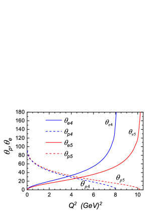
Figure 1: (Color online) Electron scattering angle $\theta_{e}$ and proton scattering angle $\theta_{p}$ versus $Q^{2}$ at the electron beam energies used in the experiment Liyanage2020 . The $\theta_{e4},\theta_{p4}$, and $\theta_{e5},\theta_{p5}$ lines are plotted for $E_{1}=4.725$ and $5.895$ GeV.

Table 1: Electron scattering angle $\theta_{e}$ and proton scattering angle $\theta_{p}$ (in radians) in the kinematics of experiment Liyanage2020

$E_{1}$ (GeV)	$Q^{2}$ (GeV2)	$\theta_{e}\,(rad)$	$\theta_{p}\,(rad)$	$Q^{2}_{max}$ (GeV)2
5.895	2.06	0.27	0.79	10.247
5.895	5.66	0.59	0.43	10.247
4.725	2.06	0.35	0.76	8.066
4.725	5.66	0.86	0.35	8.066

The data on the electron and proton scattering angles (in radians) at electron beam energies $E_{1}=5.895$ and 4.725 GeV and $Q^{2}=2.06$ and 5.66 GeV² are listed in Table 1, which contains also the values of $Q^{2}_{max}$ (29) for the maximally possible $Q^{2}$ values at $E_{1}=5.895$ and 4.725 GeV.

Polarization of the virtual photon in the $ep\to ep$ process. The $\varepsilon$ value entering the expression for the Rosenbluth cross section,

$$\varepsilon=(1+2(1+\tau_{p})\tan^{2}(\theta_{e}/2))^{-1}$$ (31)

with the range of variation $0\leqslant\varepsilon\leqslant 1$ is generally identified in the literature with the degree of longitudinal polarization of the virtual photon. Sometimes it is also referred to as the polarization parameter or simply the virtual photon polarization. The physical meaning of the $\varepsilon$ value is rarely understood correctly; in this context we should the absolutely correct words from Gakh2008 : “Let us introduce another set of kinematical variables: $Q^{\,2}$, and the degree of the linear polarization of the virtual photon, $\varepsilon$”.

Expression (31) for $\varepsilon$ is a function of the electron scattering angle $\theta_{e}$. An expression for $\varepsilon$, which differs from (31) and makes it possible to calculate the dependences of the quantities of interest on, e.g., $Q^{2}$ or the proton scattering angle $\theta_{p}$, is given below; it was derived using the results of GL97 :

$$\varepsilon^{-1}=1+\frac{(E_{1}-E_{2})^{2}+2(E_{1}-E_{2})M}{2E_{1}E_{2}-(E_{1}-E_{2})M}\,.$$ (32)

Here, $E_{1},E_{2}$ are the energies of the initial and final electrons, respectively. Note that Eqs. (23) and (24) must be used for $E_{2}$; they depend explicitly on only $Q^{2}$; in turn, the dependence of $Q^{2}$ on the angles $\theta_{e}$ and $\theta_{p}$ is determined by Eqs. (22) and (26).

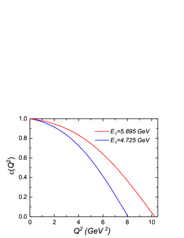
Figure 2: (Color online) $Q^{2}$-dependence of the degree of linear polarization of the virtual photon, $\varepsilon$ (32), for the electron beam energies of $4.725$ and $5.895$ GeV, used in the experiment Liyanage2020 .

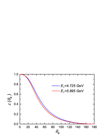
Figure 3: (Color online) Degree of linear polarization of the virtual photon, $\varepsilon$, versus the (left panel) electron scattering angle $\theta_{e}$ and (right panel) proton scattering angle $\theta_{p}$ (in degrees) at the electron beam energies of $5.895$ and $4.725$ GeV, used in the experiment Liyanage2020 .

The dependence of the degree of linear (transverse) polarization $\varepsilon$ (32) of the virtual photon on the squared momentum transfer to the proton, $Q^{2}$, at the electron beam energies used in SANE’s experiment Liyanage2020 is presented in Fig. 2.

It follows from Fig. 2 that $\varepsilon$ is a function of $Q^{2}$, which decreases from $1$ to $0$. In the case of electron scattered forward ($\theta_{e}=0^{\circ}$), when $Q^{2}=0$, $\varepsilon=1$; for a backscattered electron ($\theta_{e}=180^{\circ}$), when $Q^{2}=Q^{2}_{max}$, $\varepsilon=0$. The $Q^{2}_{max}$ values for the energies $E_{1}=4.725$ and $5.895$ GeV are listed in Table 1; they amount to $8.066$ and $10.247$ GeV², respectively. Specifically at these points, the lines in Fig. 2 intersect the abscissa axis.

Figure 3 presents the dependence of the degree of linear polarization of the virtual photon ($\varepsilon$) on the electron and proton scattering angles ($\theta_{e}$ and $\theta_{p}$, respectively) at the electron beam energies used in SANE’s experiment Liyanage2020 . Note that the angle $\theta_{e}$ in the left panel of Fig. 3 changes from $0^{\circ}$ to $180^{\circ}$, while in the right panel $\theta_{p}$ changes from $90^{\circ}$ to $0^{\circ}$. This order of counting the angles $\theta_{e}$ and $\theta_{p}$ corresponds to the range of variation $0\leqslant Q^{2}\,\leqslant Q^{2}_{max}$ for each plot.

The following regularities can be established based on the plots in Fig. 3: a smaller (larger) $\varepsilon$ value corresponds to a higher electron beam energy $E_{1}$ for the same angle $\theta_{e}$ ($\theta_{p}$).

Angular dependence of the polarization transfer to the proton in the $e\vec{p}\to e\vec{p}$ process. In the laboratory reference frame, the degree of the longitudinal polarization transfer from the initial to the final proton in process (3) in the case of a proton target partially polarized along the direction of motion of detected recoil proton is determined by Eq. (17). Currently, the experiment aimed at measuring this parameter appears to be quite real, because such a target with a high degree of polarization, $P_{t}=(70\pm 5)$ %, was in principle developed and even used in SANE’s experiment Liyanage2020 . For this reason it would be most expedient to perform the proposed experiment on the facility used in Liyanage2020 at the same value $P_{t}=0.70$, electron beam energies $E_{1}=4.725$ and 5.895 GeV, and squared momentum transfers to the proton $Q^{2}=2.06$ and 5.66 GeV². The difference between the proposed experiment and the experiment Liyanage2020 is that the electron beam must be unpolarized, and the detected recoil proton with longitudinal polarization must move strictly along the spin quantization axis of the proton target. This condition stems from the requirements imposed on the spin quantization axis for both the initial and final protons (5). The procedure of measuring the degrees of longitudinal and transverse polarizations of the final proton was developed and applied in the experiments Jones00 ; Gay01 ; Gay02 ; Pun05 ; Puckett10 ; Puckett12 . To derive the $R$ ratio (18) in the proposed experiment, one must only measure the degree of longitudinal polarization of the recoil proton, which is an advantage in comparison with the method Rekalo74 used in Jones00 ; Gay01 ; Gay02 ; Pun05 ; Puckett10 ; Puckett12 .

The calculated dependences of the longitudinal polarization transfer to the proton, $P_{r}$ (17), on the proton scattering angle $\theta_{p}$ for the electron beam energies of $5.895$ and $4.725$ GeV and for $P_{t}=0.70$ are plotted in Fig. 4. Figure 4a shows the dependence in the entire range of variation in the angles $\theta_{p}\in(90^{\circ},0^{\circ})$. In Fig. 4b the range of variation $\theta_{p}\in(47^{\circ},18^{\circ})$ corresponds to the kinematics of the experiment Liyanage2020 , where $2.06\;\rm{GeV^{2}}\leqslant Q^{2}\,\leqslant 5.66$ GeV² (see Table 1). The $Pd5$, $Pk5$, and $Pj5$ ($Pd4$, $Pk4$, and $Pj4$) lines correspond to the electron beam energy $E_{1}=5.895$ ($E_{1}=4.725$) GeV. In turn, the $Pd5$ and $Pd4$ lines were plotted for $R=R_{d}$ (19) for the case of dipole dependence; the $Pk5$ and $Pk4$ lines correspond to the Kelly parameterization Kelly2004 ($R=R_{k}$); and the $Pj5$ and $Pj4$ lines were plotted for $R=R_{j}$ (20) in the case of the Qattan parameterization Qattan2015 .

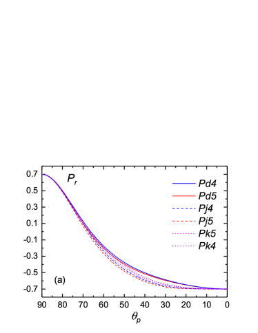
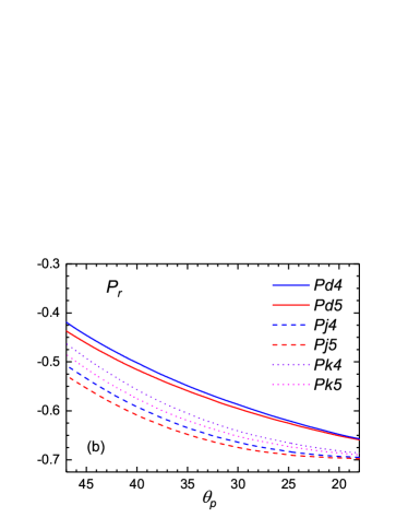
Figure 4: (Color online) (a) Dependence of $P_{r}$ (17) on the proton scattering angle $\theta_{p}$ for the $E_{1}$ and $P_{t}$ values used in the experiment Liyanage2020 in the entire range of variation in the angle $\theta_{p}\in(90^{\circ},0^{\circ})$. (b) The same dependence in the range $\theta_{p}\in(47^{\circ},18^{\circ})$, in which $2.06\,\rm{GeV}^{2}\leqslant Q^{2}\,\leqslant 5.66$ GeV². The $Pd$, $Pj$, and $Pk$ lines correspond to the dipole dependence (19), the Qattan parameterization (20) Qattan2015 , and the Kelly parameterization Kelly2004 .

Table 2: Degree of longitudinal polarization of the recoil proton $P_{r}$ (17) at electron beam energies $E_{1}=5.895$ and $4.725$ GeV and values $Q^{2}=2.06$ and 5.66 GeV². The values in the columns for $Pd$, $Pj$, and $Pk$ correspond to the dipole dependence (19), the Qattan parameterization (20) Qattan2015 , and the Kelly parameterization Kelly2004 . The corresponding electron and proton scattering angles (in degrees) are given in the columns for $\theta_{e}$ and $\theta_{p}$

$E_{1}$ (GeV)	$Q^{2}$ (GeV2)	$\theta_{e}$ (deg)	$\theta_{p}$ (deg)	$Pd$	$Pj$	$Pk$	$\Delta_{dj}$, %	$\Delta_{dk}$, %
5.895	2.06	15.51	45.23	–0.460	–0.552	–0.511	16.6	9.98
5.895	5.66	33.57	24.48	–0.628	–0.691	–0.675	9.1	6.96
4.725	2.06	19.97	43.27	–0.467	–0.556	–0.517	16.1	9.67
4.725	5.66	49.50	19.77	–0.649	–0.693	–0.682	6.4	4.84

It follows from the plots in Fig. 4 that the polarization transfer to the proton depends fairly strongly on the type of the $R$ parameterization. In the case of SFF scaling violation, i.e., at $R=R_{k}$ and $R=R_{j}$, it essentially increases in magnitude in comparison with the case of dipole dependence, when $R=R_{d}$; the following inequalities are valid for all $\theta_{p}$ in this case: $|Pd5|<|Pk5|<|Pj5|$ and $|Pd4|<|Pk4|<|Pj4|$. Thus, the $Pk$ lines for the Kelly parameterization Kelly2004 occupy an intermediate position between $Pd$ and $Pj$.

To estimate quantitatively the difference between $Pj$, $Pk$, and $Pd$, Table 2 was compiled, which contains the degrees of the longitudinal polarization of the final proton, $Pj5$, $Pd5$, $Pj4$, $Pd4$, $Pk5$, and $Pk4$, and their relative differences (in percent) $\Delta_{dj}$ and $\Delta_{dk}$

$$\Delta_{dj}=\Big{|}\frac{\rm{Pd}-\rm{Pj}}{\rm{Pd}}\Big{|},\;\Delta_{jk}=\Big{|}\frac{\rm{Pj}-\rm{Pk}}{\rm{Pj}}\Big{|}$$

at two electron beam energies (5.895 and 4.725 GeV) and two $Q^{2}$ values (2.06 and 5.66 GeV²).

It follows from Table 2 that, at $Q^{2}=2.06$ GeV², the relative difference between $Pj5$ and $Pd5$ is 16.6 %; the difference between $Pj4$ and $Pd4$ is approximately the same: 16.1 %. At $Q^{2}=5.66$ GeV² this difference decreases to $9.1$ and $6.4$ %, respectively.

The difference between $\Delta_{dj}$ and $\Delta_{dk}$ in Table 2 is small; it varies from 2 to 6 %. This difference can be explained by the fact that the Kelly parameterization Kelly2004 was proposed in 2004, prior to the experiments Puckett10 ; Puckett12 , whose results were taken into account in Qattan2015 and made it possible to obtain a more accurate parameterization.

Conclusions. Proceeding from the results of JLab’s polarization experiments on measuring the ratio of the Sachs form factors in the $\vec{e}p\to e\vec{p}$ process, using the Kelly Kelly2004 (2004) and Qattan Qattan2015 (2015) parameterizations for this ratio, in the kinematics of SANE’s experiment Liyanage2020 (2020) on measuring the double spin asymmetry in the $\vec{e}\vec{p}\to ep$ process, a numerical analysis of the dependence of the longitudinal polarization transfer to the proton in the $e\vec{p}\to e\vec{p}$ process on the proton scattering angle was performed for the case where the initial (at rest) proton is partially polarized along the direction of motion of the detected recoil proton. It has been found that the polarization transfer to the proton is fairly sensitive to the parameterization of the ratio of the Sachs form factors, which opens possibilities for a new measurement of this ratio in the $e\vec{p}\to e\vec{p}$ process.

It follows from the calculations that the violation of the scaling of the Sachs form factors leads to a significant increase in the magnitude of the polarization transfer to the proton, $|P_{r}|$, as compared to the case of the dipole dependence; the $|P_{r}|$ value, obtained with the Kelly parameterization Kelly2004 is between the results obtained for the dipole dependence and Qattan parameterization Qattan2015 . Obviously, the parameterization Qattan2015 , being based on a wider set of experimental data in comparison with the Kelly parameterization, including, in particular, the results reported in Puckett10 ; Puckett12 , is more accurate and objective and leads to small differences from the results obtained with the Kelly parameterization.

References

- (1) M. N. Rosenbluth, Phys. Rev. 79, 615 (1950).
- (2) N. Dombey, Rev. Mod. Phys. 41, 236 (1969).
- (3) A. I. Akhiezer and M. P. Rekalo, Sov. J. Part. Nucl. 4, 277 (1974) (Phys. Element. Chastits Atom. Yadra. 4, 662 (1973) [in Russian]).
- (4) A. I. Akhiezer and M. P. Rekalo, Hadron Electrodynamics (Naukova Dumka, Kiev, 1977) [in Russian].
- (5) M. V. Galynskii and M. I. Levchuk, Phys. At. Nucl. 60, 1855 (1997) (Yad. Fiz. 60, 2028 (1997) [in Russian]).
- (6) S. Pacetti, R. Baldini Ferroli, and E. Tomasi-Gustafsson, Phys. Rept. 550-551, 1 (2015).
- (7) V. Punjabi, C. F. Perdrisat, M. K. Jones, E. J. Brash, and C. E. Carlson, Eur. Phys. J. A 51, 79 (2015).
- (8) M. K. Jones, K. A. Aniol, F. T. Baker et al. (The Jefferson Lab Hall A Collaboration), Phys. Rev. Lett. 84, 1398 (2000).
- (9) O. Gayou, K. Wijesooriya, A. Afanasev et al. (The Jefferson Lab Hall A Collaboration), Phys. Rev. C 64, 038202 (2001).
- (10) O. Gayou, K.A. Aniol, T. Averett et al. (The Jefferson Lab Hall A Collaboration), Phys. Rev. Lett. 88, 092301 (2002).
- (11) V. Punjabi, C. F. Perdrisat, K. A. Aniol et al. (The Jefferson Lab Hall A Collaboration), Phys. Rev. C 71, 055202 (2005)
- (12) A. J. R. Puckett, E. J. Brash, M. K. Jones et al., Phys. Rev. Lett. 104, 242301 (2010).
- (13) A. J. R. Puckett, E. J. Brash, O. Gayou et al. (The Jefferson Lab Hall A Collaboration), Phys. Rev. C 85, 045203 (2012).
- (14) A. J. R. Puckett, E. J. Brash, M. K. Jones et al., Phys. Rev. C 96, 055203 (2017).
- (15) I. A. Qattan, J. Arrington, R. E. Segel et al., Phys. Rev. Lett. 94, 142301 (2005).
- (16) A. Liyanage, W. Armstrong, H. Kang et al. (SANE Collaboration), Phys. Rev. C 101, 035206 (2020).
- (17) T.W. Donnelly and A. S. Raskin, Ann. Phys. 169, 247 (1986).
- (18) M. V. Galynskii, E. A. Kuraev, and Yu. M. Bystritskiy, JETP Lett. 88, 481 (2008), arXiv:0805.0233 [hep-ph] (Pisma Zh. Eksp. Teor. Fiz. 88, 555 (2008) [in Russian]).
- (19) M.V. Galynskii, JETP Lett. 109, 1 (2019), arXiv: 1910.05267 [hep-ph] (Pisma Zh. Eksp. Teor. Fiz. 109, 3 (2019) [In Russian]).
- (20) M.V. Galynskii and R.E. Gerasimov, JETP Lett. 110, 646 (2019), arXiv:2004.07896 [hep-ph] (Pisma Zh. Eksp. Teor. Fiz. 110, 645 (2019) [In Russian]).
-
(21)
M.V. Galynskii,
JETP Lett. 113, 555 (2021),
arXiv:2107.08503 [hep-ph]
(Pisma Zh. Eksp. Teor.
Fiz. 113, 579 (2021) [In Russian]). - (22) M. V. Galynskii, Phys. Part. Nucl. Lett. 19, 26 (2022), arXiv:2112.12022 [nucl-ex].
- (23) J. J. Kelly, Phys. Rev. C 70, 068202 (2004).
- (24) I. A. Qattan, J. Arrington, and A. Alsaad, Phys. Rev. C 91, 065203 (2015).
- (25) A. I. Akhiezer and V. B. Berestetskii, Quantum Electrodynamics, 3rd ed. (Nauka, Moscow, 1969; Wiley, New York, 1965)
- (26) V. B. Berestetskii, E. M. Lifshits, and L. P. Pitaevskii, Course of Theoretical Physics, Vol. 4: Quantum Electrodynamics (Nauka, Moscow, 1989; Pergamon, Oxford, 1982).
- (27) A. J. R. Puckett, arXiv: nucl-ex/1508.01456.
- (28) G. I. Gakh, E. Tomasi-Gustafsson, Nucl. Phys. A 799, 127 (2008).