“Capillary” structures in transversely trapped nonlinear optical beams

Abstract

A mathematical analogy between paraxial optics with two circular polarizations of light in a defocusing Kerr medium with positive dispersion, binary Bose-Einstein condensates of cold atoms in the phase separation regime, and hydrodynamics of two immiscible compressible liquids can help in theoretical search for unknown three-dimensional coherent optical structures. In this work, transversely trapped (by a smooth profile of the refractive index) light beams are considered and new numerical examples are presented, including a “floating drop”, a precessing longitudinal optical vortex with an inhomogeneous profile of filling with the second component, and the combination of a drop and a vortex filament. Filled vortices that are perpendicular to the beam axis and propagate at large distances have also been simulated.

V. P. Ruban, JETP Lett. 117(4), 292 (2023); DOI: 10.1134/S0021364022603311

Introduction

As known, equations of paraxial optics describing the propagation of two interacting circular polarizations of light in a dielectric medium with Kerr nonlinearity [1-4] in the completely defocusing case are mathematically equivalent to the coupled Gross-Pitaevskii equations for a binary Bose-Einstein condensate in the spatial phase separation regime [5-11]. In turn, the behavior of Bose-Einstein condensates at relatively large scales in many respects corresponds to classical hydrodynamics. A number of phenomena similar to the behavior of classical immiscible liquids were theoretically revealed in the physics of ultracold gas mixtures. In particular, the effective surface tension [8, 12] is responsible for “capillary” phenomena such as bubble dynamics [13], analogs of classical hydrodynamic instabilities (Kelvin-Helmholtz [14-16], Rayleigh-Taylor [17-19], and Plateau-Rayleigh [20]), parametric instability of capillary waves at the interface [21, 22], complex textures in rotating binary condensates [23-25], three-dimensional topological structures [26-29], capillary buoyancy of droplets in trapped immiscible Bose-Einstein condensates [30], and vortices with a filled core [7, 31-38]. Many of these phenomena should occur in nonlinear optics, but some of them have not yet been observed in optical laboratories. However, at least domains of polarization of light have been known for a long time (see [39, 40] for counterpropagating waves and [41-45] for codirectional waves).

The concept of surface tension allows the qualitative analysis of many such structures, which is particularly valuable for three-dimensional configurations. This concept corresponds to the regime of extremely strong nonlinearity and is sometimes an indispensable tool for study besides the hydrodynamic approximation. In this work, using recent achievements in the field of cold gases and the common intuitive understanding of the properties of capillarity based on daily practice, some important aspects of filled optical vortices, which are known two-component objects, were examined [43-47]. Furthermore, three likely novel capillary structures in transversely trapped optical beams — simple floating drop, precessing floating drop with longitudinal vortex filaments attached to it, and filled vortices perpendicular to the beam axis — are “constructed” numerically.

Model

A fundamentally insignificant difference of optics from hydrodynamics is that the evolutionary variable in optics is usually the distance $\zeta$ along the beam axis rather than the time $t$, and the “delayed” time $\tau=t-\zeta/v_{\rm gr}$ serves as the third “spatial” coordinate. For this reason, some effort is sometimes required to realize the four-dimensional picture of a phenomenon. In particular, this remark concerns the motion of quantized vortices, which can have different orientations in the $(x,y,\tau)$ space.

We consider a dielectric medium with an isotropic dispersion relation of linear optical waves $k(\omega)=\sqrt{\varepsilon(\omega)}\omega/c$ and with defocusing Kerr nonlinearity. Let the dispersion of the group velocity be anomalous (i.e., $k^{\prime\prime}(\omega)<0$ in a certain range). We fix the carrier frequency $\omega$, the corresponding wavenumber $k_{0}$, and the second derivative $k_{0}^{\prime\prime}$. We also assume that the part of the permittivity linear in the electric field in the spatial region of interest is slightly inhomogeneous and has an approximately parabolic two-dimensional profile at the frequency $\omega$:

$$\varepsilon_{\rm lin}=\varepsilon[1+\nu^{2}(2-(x^{2}+\kappa^{2}y^{2})/R^{2})],$$ (1)

where $\nu\ll 1$ is a small dimensionless parameter, $R\gg 1/k_{0}$ is the relatively large length parameter (characteristic width of the light beam), and $\kappa$ is the coefficient specifying the transverse geometric anisotropy of such a smooth waveguide (for certainty, $\kappa\geq 1$). A similar medium was considered, e.g., in [48] (for one polarization of light).

Below, the optical beam with both circular polarizations is considered. In terms of the appropriate dimensionless variables, the system of equations for slow complex envelopes $A_{1,2}(x,y,\tau,\zeta)$ corresponding to the right and left circular polarizations of light has the form

$$i\frac{\partial A_{1,2}}{\partial\zeta}=\Big{[}-\frac{1}{2}\Delta+V(x,y)+|A_{1,2}|^{2}+g_{12}|A_{2,1}|^{2}\Big{]}A_{1,2},$$ (2)

where $\Delta=\partial_{x}^{2}+\partial_{y}^{2}+\partial_{\tau}^{2}$ is the three-dimensional Laplace operator in the $(x,y,\tau)$ “coordinate” space. These equations are easily derived by analogy with the section “Self-focusing” in L.D. Landau and E.M. Lifshitz, Electrodynamics of Continuous Media (Pergamon, Oxford, 1984). To this end, the expression for the electric field in terms of circular polarizations

$${\bf E}=\big{[}({\bf e}_{x}+i{\bf e}_{y})A_{1}+({\bf e}_{x}-i{\bf e}_{y})A_{2}\big{]}/\sqrt{2}$$ (3)

should be substituted into the formula

$${\bf D}^{(3)}=\alpha(\omega)|{\bf E}|^{2}{\bf E}+\beta(\omega){\bf E}^{2}{\bf E}^{*},$$ (4)

the remaining algebra should be performed (taking into account the second time derivative), and the following rescaling should be done: $\zeta=(\nu/R)\cdot\zeta_{\rm old}$, $\{x,y\}=\sqrt{\nu k_{0}/R}\cdot\{x,y\}_{\rm old}$, $\tau=\sqrt{\nu/(R|k_{0}^{\prime\prime}|)}\cdot\tau_{\rm old}$, and $A_{1,2}=\sqrt{k_{0}R|\alpha|/(2\nu\varepsilon)}\cdot A_{1,2}^{(\rm old)}$.

It is noteworthy that the corresponding equations obtained in the basis of linearly or elliptically polarized waves will include additional terms with four-wave mixing, which is less convenient for analysis. Nonlinearity is defocusing if $\alpha$ and $\beta$ are negative. The cross-phase modulation parameter $g_{12}=1+2\beta/\alpha$ depends on the material; in a typical case, it is 2. The defocusing character of nonlinearity and the condition of strong cross repulsion $g_{12}>1$ imply the phase separation regime. In other words, domains with opposite circular polarizations are spontaneously formed at intensities of light $|A_{1,2}|^{2}\sim I$ in the $(x,y,\tau)$ space at scales $l\gg 1/\sqrt{I}$ [41-45]. The initial stage of this process is often a specific modulation instability of states with linear or elliptic polarization. The geometric shape of these domains changes generally with increasing $\zeta$, which corresponds to time evolution in hydrodynamics. The thickness $w\sim 1/\sqrt{I}$ of domain walls in this case is about the inverse typical amplitude and the surface tension is $\sigma\sim I^{3/2}$.

The effective external potential $V(x,y)$ in Eqs. (2) is proportional to the deviation $\tilde{\varepsilon}(x,y)$ of the permittivity from a constant value taken with the minus sign. In our case,

$$V(x,y)=(x^{2}+\kappa^{2}y^{2})/2-\mu,\qquad\mu=\nu k_{0}R.$$ (5)

Inhomogeneity $\tilde{\varepsilon}$ is necessary for the transverse confinement of the optical beam undergoing diffraction and nonlinear defocusing. The refractive index can generally depend on $\zeta$, but this dependence should be sufficiently slow for the physical applicability of the approximation under consideration. For the validity of analogy with optics in the case of Bose-Einstein condensates, the potential of the trap should depend on no more than two Cartesian space coordinates and possibly on the time. Below, we focus on the purely two-dimensional potential “valley” given by Eq. (5). In “equilibrium,” when the functions $A_{1}$ and $A_{2}$ are independent of $\zeta$, the length of the light beam in the variable $\tau$ is thus infinite. This property implies that possible two-dimensional solutions (independent of $\tau$) should be unstable because a stable longitudinal domain wall can hardly be realized in this situation; domains with transverse walls alternating along the $\tau$ axis seem more realistic. At the same time, the increment of longitudinal instability will be very small for long-wavelength (i.e., low-frequency) perturbations, and their amplitudes will increase strongly only at fairly large $\zeta$ values when many events occur in two-dimensional dynamics.

The parameter $\mu$ (in the theory of Bose-Einstein condensates, it is the dimensionless chemical potential) will characterize the level of nonlinearity of the background state of the optical field ($I_{1}\sim\mu$). It is assumed to be large enough for the transverse dimension of the beam $R_{\perp}\sim\sqrt{\mu}$ to be much larger than the characteristic thickness of domain walls $w$ and the core $\xi$ of quantized vortices: $w\sim\xi\sim 1/\sqrt{\mu}$. At the same time, overly high powers can be undesirable in practice. For this reason, the moderate value $\mu=6.0$ is used in numerical examples.

The parameter $\nu$ should be small to ensure the applicability of the quasimonochromatic approximation because the characteristic width of vortices and domain walls in the initial dimensional variables is estimated as $w_{\perp}\sim(\nu k_{0})^{-1}\gg 1/k_{0}$ in the transverse coordinates and as $w_{\tau}\sim\sqrt{|k_{0}^{\prime\prime}|/k_{0}}/\nu$ in the time coordinate. Therefore, (anomalous) dispersion should not be too weak to ensure the condition $w_{\tau}\gg 1/\omega$ .

Realistic parameters seem to be $\nu\sim 0.03$ and $k_{0}R\sim 200$, which constitutes about 30 wavelengths (then, about five wavelengths in the thickness of vortices and domain walls). The characteristic distance along the beam $R/\nu$ is about a thousand wavelengths, i.e., about a millimeter. The $\zeta$ interval of several hundred units corresponds to tens of centimeters. The system under consideration is in principle similar to graded-index multimode optical fibers, although light beams in the latter case are narrower, only a few wavelengths (see, e.g., [49-53] and references therein). A more important difference is the defocusing character of nonlinearity in our case, whereas conventional optical fibers are made of materials with focusing nonlinearity. For this reason, a fast experimental test of predictions of the developed theory is hardly possible because special efforts are required to fabricate a sample with the necessary properties. It is important that the defocusing Kerr dielectric with anomalous dispersion and a smooth profile of the refractive index is not fundamentally forbidden (see, e.g., [48]). Since numerical solutions for such systems are very interesting, these theoretical results need serious attention.

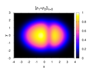
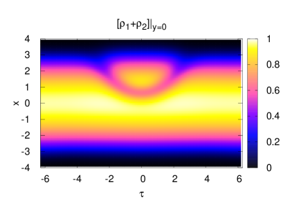
Figure 1: Numerical example of the light beam with the floating drop at the variable $\zeta=300$. Color represents the total normalized density $\rho_{1}+\rho_{2}=(I_{1}+I_{2})/\mu$ (a) in the cross section of the beam by the $\tau=0$ plane and (b) in the longitudinal section of the beam by the $y=0$ plane.

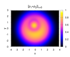
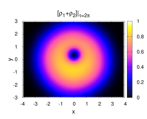
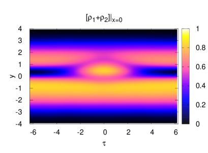
Figure 2: Light beam with the precessing vortex-soliton complex at $\kappa=1$ and $\zeta=228$: (a) the cross section of the beam by the $\tau=0$ plane, (b) the cross section of the beam by the $\tau=2\pi$ plane, and (c) the longitudinal section of the beam by the $x=0$ plane.

Numerical method

The system of Eqs. (2) was solved numerically in the cubic region $(4\pi)^{3}\approx(12.6)^{3}$ with periodic boundary conditions in variables $(x,y,\tau)$ by the second-order Fourier method with a split step in the variable $\zeta$. The accuracy of calculations was controlled by the conservation of the Hamiltonian of the system to the sixth decimal place. Nearly steady states at $\zeta=0$ were prepared by the imaginary-time propagation method. In other words, $i$ was replaced by $-1$ on the left-hand sides of Eqs. (2) and this dissipative dynamics was calculated in a certain finite pseudotime interval. In this case, a certain positive correction $\delta\mu_{2}$ was added to the chemical potential of the second component. This correction and bare profiles of both wave amplitudes were selected using the trial-and-error method to obtain the desired “mass” of the second component. This dissipative procedure strongly suppressed hard excitations, whereas soft degrees of freedom of interest remained unrelaxed. After that, the calculation of conservative system (2) began.

Several substantial numerical examples are given below.

Floating drop

We begin with the simplest case where almost the entire beam (with the transverse anisotropy parameter $\kappa^{2}=2$ ) consists of the first component where a drop of the second component floats (see Fig. 1, where the domain wall is seen as a dip of the total intensity). Quantized vortices are absent. Imaginary-time relaxation at the stage of preparation of the initial state leads to a nearly static initial configuration. The shape of the drop slightly oscillates with the conditional “time” $\zeta$. Such a behavior is intuitively clear because we deal with a natural mechanical system where the minimum of the potential energy is reached at given total masses of both components and small oscillations near this minimum occur. However, an overly massive drop is unstable and, as a result, the drop fills the entire section of the beam in a certain part of it (such a simple quasi-one-dimensional structure is not shown here).

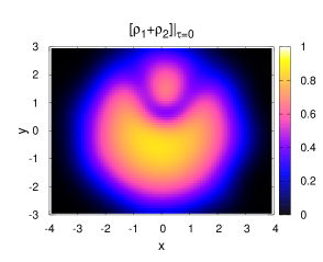
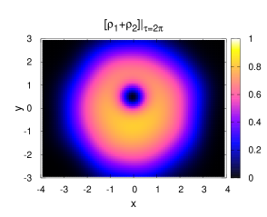
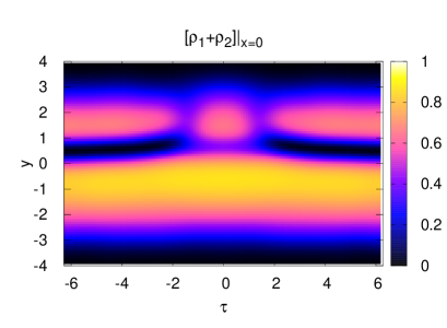
Figure 3: Precessing floating drop with attached vortex filaments at $\kappa=1$ and $\zeta=253$: (a) the cross section of the beam by the $\tau=0$ plane, (b) the cross section of the beam by the $\tau=2\pi$ plane, and (c) the longitudinal section of the beam by the $x=0$ plane.

Longitudinal vortex with inhomogeneous filling

Very interesting numerical solutions are obtained if the confining potential is axisymmetric ($\kappa=1$) and a longitudinally oriented (single) optical vortex with a filled core is located at a small distance from the beam axis at $\zeta=0$ . In the presence of small initial inhomogeneity, the so-called sausage instability is developed; it is caused by surface tension and results in the formation of a spindle-shaped bubble with attached input and output vortex filaments (this phenomenon was discussed in [36]). In the case of a moderate amount of the second component, the formation and decay of the bubble can be repeated several times. In this case, the vortex precesses about the beam axis. The vortex with a sufficiently appropriate inhomogeneous filling can immediately be initiated; in this case, the bubble approximately keeps its shape, rotating about the beam axis (see video [54], where the dynamics of the conditional surface determining the core of the vortex is shown; color corresponds to the $x$ coordinate). Thus, the sausage instability is saturated and a precessing three-dimensional vortex-soliton complex is formed, exemplified in Fig. 2. It is seen that the length of the second component along the beam is finite: it is entirely “extruded” by the surface tension from the remaining part of the vortex to the bubble. Since this complex in the numerical experiment expands to hundreds of units in the variable $\zeta$ and is held under “unsteady” perturbations, it is assumingly stable. However, this problem requires further study. This example is a nontrivial generalization of the structure previously known for a uniform medium (without the confining external potential) [43–47].

It should be mentioned that, if a certain longitudinal “velocity” $u$ is assigned to the second component at $\zeta=0$ (multiplying $A_{2}$ by $\exp(iu\tau)$, which really means a small reduction of the frequency of the second component), the soliton becomes moving and the entire structure becomes slightly twisted (see video [55]).

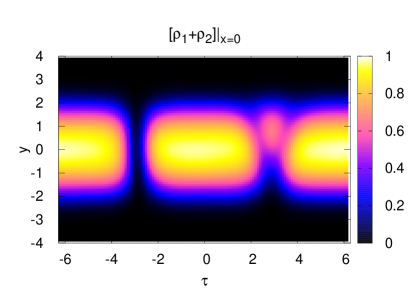
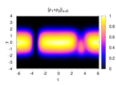
Figure 4: System of two transverse vortices at $\kappa^{2}=2$. The positive and negative vortices are oriented along the $y$ axis and their cores differ in the amount of the trapped second component. The longitudinal section of the beam by the $x=0$ plane at $\zeta=$ (a) 291 and (b) 300.

Floating drop with attached vortex filaments

The scenario of evolution at the quite large filling of the initial vortex is different. In this case, a massive lemon-shaped bubble is formed on the vortex and, then, its precession becomes unstable. The bubble floats to the surface of the beam and is transformed to a floating drop with two empty vortex filaments attached to it. After transient processes, the system again undergoes almost stationary precession about the beam axis (see video [56]). The corresponding example is shown in Fig. 3. Such a complex solution obviously cannot be obtained by any existing analytical methods. However, being constructed numerically, this solution seems natural and convincing.

Transverse vortices with filling

Finally, we examine the possibility that vortices in the general case can be oriented arbitrarily in the $(x,y,\tau)$ space, in particular, across the beam. The calculations showed that such transverse configurations are long-lived. Figure 4 presents the situation with two opposite transverse vortices; the second vortex is necessary to satisfy the periodic boundary condition in the variable $\tau$. One of the vortices is filled and the second is almost empty. The distance between the vortices in this numerical experiment was periodically varied but without their close approach (see video [57]). Moreover, since the center of masses of the second component was first above the $y=0$ plane, slow vibrations of the second component along the $y$ axis occur in the process of propagation. These vertical vibrations are seen in Fig. 4.

Dynamics in the presence of a larger number of such vortices has not yet been simulated because this simulation would require a sufficiently long computational region in the variable $\tau$. This problem remains for future studies.

It is interesting to note that a sequence of such transverse vortices can carry information because the filling of each vortex holds for a long time and can be used for encoding. It is still unclear whether this property can be used in practice.

Conclusions

To summarize, the concept of surface tension has been applied to nonlinear and unsteady optical beams with both circular polarizations. A number of new significantly three-dimensional combined coherent structures caused by phase separation have been found.

This field of research seems quite promising because almost any reasonable initial configuration leads to interesting subsequent dynamics. In particular, the simulation of the interaction of two floating drops coupled by a vortex filament, as well as the consideration of the dynamics of polarization domains in the presence of transverse vortices against a significantly nonparabolic background intensity profile [e.g., in the two-well potential $V(x,y)$], remains for the future.

It is noteworthy that the interaction between two polarizations leads to interesting structures in systems with more complex nonlinearity as well (see, e.g., [58, 59]).

A certain time is required to verify whether the predicted solutions will be implemented experimentally. As mentioned above, this is hardly possible with existing samples, and appropriate experimental materials should be prepared from the “beginning”.

Funding

This work was supported by the Ministry of Science and Higher Education of the Russian Federation (state assignment no. 0029-2021-0003).

Conflict of interest

The author declares that he has no conflicts of interest.

Open access

This article is licensed under a Creative Commons Attribution 4.0 International License, which permits use, sharing, adaptation, distribution and reproduction in any medium or format, as long as you give appropriate credit to the original author(s) and the source, provide a link to the Creative Commons license, and indicate if changes were made. The images or other third party material in this article are included in the article’s Creative Commons license, unless indicated otherwise in a credit line to the material. If material is not included in the article’s Creative Commons license and your intended use is not permitted by statutory regulation or exceeds the permitted use, you will need to obtain permission directly from the copyright holder. To view a copy of this license, visit
http://creativecommons.org/licenses/by/4.0/ .

References

- (1) A. L. Berkhoer and V. E. Zakharov, Sov. Phys. JETP 31, 486 (1970).
- (2) Y. Kivshar and G. P. Agrawal, Optical Solitons: From Fibers to Photonic Crystals, (Academic, San Diego, CA, 2003).
- (3) V. E. Zakharov and S. Wabnitz, Optical Solitons: Theoretical Challenges and Industrial Perspectives (Springer, Berlin, 1999).
-
(4)
B. A. Malomed, Multidimensional Solitons
(AIP, Melville, N. Y., 2022)
https://doi.org/10.1063/9780735425118 - (5) Tin-Lun Ho and V. B. Shenoy, Phys. Rev. Lett. 77, 3276 (1996).
- (6) H. Pu and N. P. Bigelow, Phys. Rev. Lett. 80, 1130 (1998).
- (7) B. P. Anderson, P. C. Haljan, C. E. Wieman, and E. A. Cornell, Phys. Rev. Lett. 85, 2857 (2000).
- (8) S. Coen and M. Haelterman, Phys. Rev. Lett. 87, 140401 (2001).
- (9) G. Modugno, M. Modugno, F. Riboli, G. Roati, and M. Inguscio, Phys. Rev. Lett. 89, 190404 (2002).
- (10) E. Timmermans, Phys. Rev. Lett. 81, 5718 (1998).
- (11) P. Ao and S. T. Chui, Phys. Rev. A 58, 4836 (1998).
- (12) B. Van Schaeybroeck, Phys. Rev. A 78, 023624 (2008).
- (13) K. Sasaki, N. Suzuki, and H. Saito, Phys. Rev. A 83, 033602 (2011).
- (14) H. Takeuchi, N. Suzuki, K. Kasamatsu, H. Saito, and M. Tsubota, Phys. Rev. B 81, 094517 (2010).
- (15) N. Suzuki, H. Takeuchi, K. Kasamatsu, M. Tsubota, and H. Saito, Phys. Rev. A 82, 063604 (2010).
- (16) H. Kokubo, K. Kasamatsu, and H. Takeuchi, Phys. Rev. A 104, 023312 (2021).
- (17) K. Sasaki, N. Suzuki, D. Akamatsu, and H. Saito, Phys. Rev. A 80, 063611 (2009).
- (18) S. Gautam and D. Angom, Phys. Rev. A 81, 053616 (2010).
- (19) T. Kadokura, T. Aioi, K. Sasaki, T. Kishimoto, and H. Saito, Phys. Rev. A 85, 013602 (2012).
- (20) K. Sasaki, N. Suzuki, and H. Saito, Phys. Rev. A 83, 053606 (2011).
- (21) D. Kobyakov, V. Bychkov, E. Lundh, A. Bezett, and M. Marklund, Phys. Rev. A 86, 023614 (2012).
- (22) D. K. Maity, K. Mukherjee, S. I. Mistakidis, S. Das, P. G. Kevrekidis, S. Majumder, and P. Schmelcher, Phys. Rev. A 102, 033320, (2020).
- (23) K. Kasamatsu, M. Tsubota, and M. Ueda, Phys. Rev. Lett. 91, 150406 (2003).
- (24) K. Kasamatsu and M. Tsubota, Phys. Rev. A 79, 023606 (2009).
- (25) P. Mason and A. Aftalion, Phys. Rev. A 84, 033611 (2011).
- (26) K. Kasamatsu, M. Tsubota, and M. Ueda, Phys. Rev. Lett. 93, 250406 (2004).
- (27) H. Takeuchi, K. Kasamatsu, M. Tsubota, and M. Nitta, Phys. Rev. Lett. 109, 245301 (2012).
- (28) M. Nitta, K. Kasamatsu, M. Tsubota, and H. Takeuchi, Phys. Rev. A 85, 053639 (2012).
- (29) K. Kasamatsu, H. Takeuchi, M. Tsubota, and M. Nitta, Phys. Rev. A 88, 013620 (2013).
- (30) V. P. Ruban, JETP Lett. 113, 814 (2021).
- (31) K. J. H. Law, P. G. Kevrekidis, and L. S. Tuckerman, Phys. Rev. Lett. 105, 160405 (2010); Erratum, Phys. Rev. Lett. 106, 199903 (2011).
- (32) M. Pola, J. Stockhofe, P. Schmelcher, and P. G. Kevrekidis, Phys. Rev. A 86, 053601 (2012).
- (33) S. Hayashi, M. Tsubota, and H. Takeuchi, Phys. Rev. A 87, 063628 (2013).
- (34) A. Richaud, V. Penna, R. Mayol, and M. Guilleumas, Phys. Rev. A 101, 013630 (2020).
- (35) A. Richaud, V. Penna, and A. L. Fetter, Phys. Rev. A 103, 023311 (2021).
- (36) V. P. Ruban, JETP Lett. 113, 532 (2021).
- (37) V. P. Ruban, W. Wang, C. Ticknor, and P. G. Kevrekidis, Phys. Rev. A 105, 013319 (2022).
- (38) V. P. Ruban, JETP Lett. 115, 415 (2022).
- (39) V. E. Zakharov and A. V. Mikhailov, JETP Lett. 45, 349 (1987).
- (40) S. Pitois, G. Millot, and S. Wabnitz, Phys. Rev. Lett. 81, 1409 (1998).
- (41) M. Haelterman and A. P. Sheppard, Phys. Rev. E 49, 3389 (1994).
- (42) M. Haelterman and A. P. Sheppard, Phys. Rev. E 49, 4512 (1994).
- (43) A. P. Sheppard and M. Haelterman, Opt. Lett. 19, 859 (1994).
- (44) N. Dror, B. A. Malomed, and J. Zeng, Phys. Rev. E 84, 046602 (2011).
- (45) Yu. S. Kivhsar and B. Luther-Davies, Phys. Rep. 298, 81 (1998).
- (46) A. H. Carlsson, J. N. Malmberg, D. Anderson, M. Lisak, E. A. Ostrovskaya, T. J. Alexander, and Yu. S. Kivshar, Opt. Lett. 25, 660 (2000).
- (47) A. S. Desyatnikov, L. Torner, and Yu. S. Kivshar, Progress in Optics 47, 291 (2005).
- (48) S. Raghavan and G. P. Agrawal, Opt. Communications 180, 377 (2000).
- (49) S. Longhi, Opt. Lett. 28, 2363 (2003).
- (50) A. Mafi, J. Lightwave Technology 30, 2803 (2012).
- (51) C. M. Arabi, A. Kudlinski, A. Mussot, and M. Conforti, Phys. Rev. A 97, 023803 (2018).
- (52) T. Mayteevarunyoo, B. A. Malomed, and D. V. Skryabin, J. Opt. 23, 015501 (2020).
- (53) L. G. Wright, F. O. Wu, D. N. Christodoulides, and F. W. Wise, Nat. Phys. 18, 1018 (2022).
- (54) http://home.itp.ac.ru/~ruban/27DEC2022/w1.avi
- (55) http://home.itp.ac.ru/~ruban/27DEC2022/w1a.avi
- (56) http://home.itp.ac.ru/~ruban/27DEC2022/w2.avi
- (57) http://home.itp.ac.ru/~ruban/27DEC2022/w3.avi
- (58) A. S. Desyatnikov and Yu. S. Kivshar, Phys. Rev. Lett. 87, 033901 (2001).
- (59) F. Bouchard, H. Larocque, A. M. Yao, C. Travis, I. De Leon, A. Rubano, E. Karimi, G.-L. Oppo, and R. W. Boyd, Phys. Rev. Lett. 117, 233903 (2016).