DeepCuts: Single-Shot Interpretability based Pruning for BERT

Abstract

As language models have grown in parameters and layers, it has become much harder to train and infer with them on single GPUs. This is severely restricting the availability of large language models such as GPT-3, BERT-Large, and many others. A common technique to solve this problem is pruning the network architecture by removing transformer heads, fully-connected weights, and other modules. The main challenge is to discern the important parameters from the less important ones. Our goal is to find strong metrics for identifying such parameters. We thus propose two strategies: Cam-Cut based on the GradCAM interpretations, and Smooth-Cut based on the SmoothGrad, for calculating the importance scores. Through this work, we show that our scoring functions are able to assign more relevant task-based scores to the network parameters, and thus both our pruning approaches significantly outperform the standard weight and gradient-based strategies, especially at higher compression ratios in BERT-based models. We also analyze our pruning masks and find them to be significantly different from the ones obtained using standard metrics.

1 Introduction

It has been extremely challenging to train or even at times fine-tune large language models like BERT-Large, RoBERTa-Large, BART-large, and many others on single GPU devices. Simultaneously, many applications require model deployment on less powerful devices like mobile devices and in federated learning over multiple edge devices which cannot be supported for very large language models. Thus reducing the model size and retaining as much performance as possible is essential for these applications and less resourceful users. Hence, our objective is to identify strategies and scoring functions for discerning essential weights from the less important ones with special consideration to the dataset and task in hand. This is similar to the schematic shown in 1. We thus perform single-shot pruning to compare the performance of our metrics with standard weight and gradient-based methods. We believe interpretability techniques developed for Explainable ML like GradCAM Selvaraju et al., (2017) and SmoothGrad Smilkov et al., (2017) can provide significant bases for weight identification and thus can be repurposed for pruning the weights of large language models. Recent works have leveraged the Lottery Ticket Hypothesis (LTH) Frankle and Carbin, (2018); Prasanna et al., (2020) which states that for every large model, we can identify a smaller sub-model that when trained from the same initialization will perform similarly or even at times better than the original model. But it is very difficult to efficiently identify these sub-models especially when we want them to be much smaller than the original model.

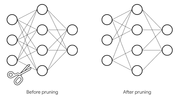
Figure 1: A schematic representation of pruning tfp, (2019).

1.1 Related Works

The pruning problem is mainly tackled using two broad categories of approaches Blalock et al., (2020). These include unstructured pruning Han et al., (2015); Gale et al., (2019), and structure-based pruning Voita et al., (2019); Zhang et al., (2021); Perez and Reinauer, (2022). Unstructured pruning involves scoring individual prunable structures for removing individual parameters from modules whereas structured pruning includes removing complete modules from the model like complete attention heads and MLP layers from transformer architectures. Other pruning methods use probability-guided pruning where probabilities are assigned to parameters based on the given scoring function and the pruning is done by sampling from this distribution Wang et al., (2017). There are also mask learning approaches that directly learn pruning masks during the training methods and use them to prune the weightsLouizos et al., (2017). Many methods in tabular machine learning also have conditions for independence of feature interactions, which also leads to smaller models used especially in financial applications like GAMI-Net Yang et al., (2021). Many works Han et al., (2015); Frankle and Carbin, (2018); Sanh et al., (2020); Prasanna et al., (2020) follow an iterative pruning and fine-tuning strategy where a certain percentage of the model is pruned in every cycle followed by fine-tuning. Other works explore single-shot pruning, i.e. pruning and training the network only once Lee et al., (2018).

Many of the existing works use magnitude-based approaches that use absolute network weights to directly assign scores to the parameters, i.e. the higher the absolute value of the parameter, the higher its importance, and the less likely it is to be pruned Frankle and Carbin, (2018); Prasanna et al., (2020). The main issue with this approach is that if many low-value parameters belong to any of the earlier layers in the network, they would be pruned and most of the information flowing through the later layers would be cut off. This issue is resolved in the existing literature Lee et al., (2020) by applying a cap on the max number of parameters that can be pruned in each layer. These works focus on the magnitude of the parameters which by themselves do not carry all the task-relevant information in hand and thus do not perform well. Many recent works Sanh et al., (2020); Zhang et al., (2021); Kurtic et al., (2022) explore the combinations of gradients and parameter values. These works explore different variants of the gradients in the scoring functions for instance some use the absolute value of gradients Zhang et al., (2021) while others consider the directions of gradients as well Sanh et al., (2020). Some works Yu et al., (2022); Kurtic et al., (2022) also explore higher-order gradients such as Hessian but their calculations could become compute and memory intensive.

Machine Learning Interpretability methods like GradCAMSelvaraju et al., (2017), Integrated Gradients Sundararajan et al., (2017), and Smooth Grad Smilkov et al., (2017) have been used to understand models in the recent past. They obtain saliency maps for computer vision and language applications Dai et al., (2021) using methods like LIME Ribeiro et al., (2016), GradCAM, SmoothGrad, and others which have been used to attribute significance to a given pixel or token for a given output. We believe that we can leverage these techniques to do the same for the parameters of the architecture that can serve as a score for pruning. Pruning and interpretability face similar challenges. In interpretability, noisy gradients have always been a challenge, and the same is also observed in pruning. Similarly, excluding the magnitude of input hinders interpretability and the same is true for parameter magnitude in pruning. However, these challenges have been addressed through SmoothGrad, and Inverted Representations Mahendran and Vedaldi, (2015) in interpretability. Simultaneously, using a combination of gradients and input image as a product has been a very common approach in the interpretability literature to identify important regions in input that contribute the most to generating the given output. The same practice is being used in pruning using the product of weight magnitude and gradient as a scoring function. Thus, we believe ideas like SmoothGrad and GradCAM can provide a very intuitive and effective foundation for scoring functions for pruning.

1.2 Our Contributions

We test our ideas by implementing an LTH-based approach to pruning on the SST-2 Socher et al., (2013), STS-B Cer et al., (2017), and CoLA Warstadt et al., (2018) datasets which are very well-known datasets in the GLUE Wang et al., (2018) NLP benchmark. We thus built Cam-Cut based on GradCAM, Smooth-Cut based on SmoothGrad, and Smooth-Cam-Cut which combined the ideas of both approaches. For measuring size reduction, we use the Compression Ratio, which is the ratio of the number of parameters in the unpruned model to the number of parameters in the pruned model. For benchmarking our results against the baselines, we used ShrinkBench Ortiz et al., (2019) which provides a standard implementation for pruning the fully-connected layers and convolutional models.

In this work, our contribution is five-fold:

• Cam-Cut: A GradCAM-based pruning metric that performs well, especially on high compression ratios.

• Smooth-Cut: A SmoothGrad-based pruning metric that performs well with noisy gradient signals.

• We outperform the baselines at different compression ratios on three GLUE datasets and discuss the results and effectiveness of our strategies.

• We compare the pruning masks for Smooth-Cut and Cam-Cut with the pruning masks for our baselines to show that these strategies identify different parameters for pruning.

• We also analyze our pruning masks to give important insights into BERT layers and parameters thus allowing a deeper understanding of the BERT model.

2 Problem Formulation

We aim to prune BERT-based models, with task-specific classification and regression layers over the BERT pooling layer for the SST-2, STS-B, and CoLA datasets. As we perform pruning, our inputs include the training dataset, the BERT model with a regressor or classifier layer, and our pruning strategy. The output is a set of pruning masks over every parameter in the model that carries information on which weights and biases are retained and which ones are pruned. We reinitialize the network parameters with pre-pruned values, and fine-tune the models with the mask applied, thus obtaining our final performance of the pruned model. Currently, we are performing single-shot unstructured pruning using the LTH for Cam-Cut, Smooth-Cut, and SmoothCam-Cut strategies. The key challenges we address involve augmenting GradCAM as Cam-Cut, and SmoothGrad as Smooth-Cut using LTH and applying them to multi-batch, multi-token sequences as interpretation methods were used only for single sequences.

We have included the standard baseline results of LayerMagWeight and GlobalMagWeight strategies as proposed in the LTH paper. To the best of our knowledge, we did not find any relevant works in single-shot unstructured pruning that provide a comprehensive review of pruning strategies for large language models. In addition, the current state-of-the-art in iterative unstructured pruning, Optimal BERT Kurtic et al., (2022) also report their single-shot performance. However, we can not compare our results with this work as they only provide GPU-specific results for 2-out-of-4 sparsity on NVIDIA Ampere GPU Mishra et al., (2021). For this, they use magnitude-based pruning strategies for benchmarking their results which is also our baseline.

2.1 Baseline Models

2.1.1 Global Magnitude Pruning

The Global Magnitude Pruning method or GlobalMagWeight method is originally proposed in the LTH paper. It uses the importance score $S$ which is computed using the network parameters $w$ as:

$$S=|w|$$ (1)

The importance score is then converted into a mask by selecting parameters with the maximum score from throughout the architecture, irrespective of the module or layer they are in. The mask is a binary tensor for every parameter tensor with 1 for all included weights and 0 for excluded ones. Thus, the mask creation for a parameter $w$ is done by:

$$mask[w]=\begin{dcases*}1,&if $w\in$ top $q$ quantile\\ &of the parameters overall,\\ 0,&otherwise.\end{dcases*}$$ (2)

where $q$ is determined using the compression ratio and a number of prunable parameters throughout the model.

2.1.2 Layer Magnitude Pruning

The Layer Magnitude Pruning method or LayerMagWeight method was originally proposed in the LTH paper as well. It uses the importance score in the same way as GlobalMagWeight. However, unlike the global magnitude implementation, the importance score is converted into a mask by selecting parameters with the maximum score from that particular module and not the entire network. The mask is a binary tensor for every parameter with 1 for all included weights and 0 for excluded ones. Thus, the mask creation for a parameter $w$ is done by:

$$mask[w]=\begin{dcases*}1,&if $w\in$ top $q$ quantile of\\ &parameters in given tensor,\\ 0,&otherwise.\end{dcases*}$$ (3)

where $q$ is determined using the compression ratio and the number of prunable parameters in the considered module.

2.2 Challenges Faced

2.2.1 Issues with baseline approaches

As seen above, the baseline methods only consider the magnitude of the weights for pruning. For zero-shot pruning, they are completely task-agnostic as the model is trained only for language modeling. However, for single-shot pruning, the weights do reflect some significance of the task at hand due to fine-tuning but the pruning metric does not reflect the same directly. We thus look into gradient-based pruning methods. One of the standard implementations in the ShrinkBench framework called LayerMagGrad used parameter magnitude and gradient as a metric as shown for the given parameter $w$:

$$S_{LayerMagGrad}=|w\times\dfrac{\partial{L}}{\partial{w}}|$$ (4)

This is similar to the Vanilla Gradient Simonyan et al., (2013) formulation in interpretability literature. Here, the gradients are known to be noisy which affects the pruning performance. In addition, these gradients are also not very good estimators of their local neighborhoods. We also verified this in our tests as only gradient-based scoring did not perform well whereas a combination of weights and gradients performed better than the baseline of only weights. A major observation was that till the compression ratio of 2, all methods performed similarly, and major gains due to gradient information are observed as we go from compression ratios of 2 to 4.

3 Implementation Details

3.1 Dataset Processing

To handle inputs for the three datasets: SST-2, STS-B, and CoLA, we use dataset-specific tokenization techniques. As SST-2 and CoLA are single text classifications, we directly tokenize them without introducing different masking and separator tokens, whereas, in the STS-B dataset, regression is done according to pair of sentences. These are separated by a separator token and different segment embeddings are provided. For STS-B regression we use sigmoid as the last layer and multiply it with $5$ to make it suitable for the $5$-level similarity regression.

3.2 Gradient Computations

All our proposed methods need a gradient of the loss with respect to the considered weight for importance and mask calculations. Thus, for computing the gradients, we break the entire training set into multiple batches and one gradient is computed per batch. This gradient is converted into the importance metric according to the selected strategy and the importance scores are accumulated over the entire dataset. This ensures that gradients over the entire dataset are considered and not over a random batch. For reducing computation, we consider the first $1,000$ batches generated from the dataset.

3.3 Prunable Layers

Currently, not all parameters of the BERT model are considered prunable. The Embedding layers are generally not considered for pruning in various works thus we have also not pruned them. Similarly, LayerNorm layers also have parameters for normalizing outputs which are not pruned. The classifier and regressor layers making the final predictions are also not being pruned currently. Thus, out of 110 million BERT parameters, only 85 million are considered prunable.

3.4 Cam-Cut (LayerGradCAMShift)

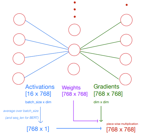
Figure 2: GradCAM for a 3-layer MLP. Here, we average the activations over the current batch to obtain a single vector, which we then multiply piece-wise with each column of the gradient matrix. The resultant matrix is then piece-wise multiplied by the magnitude of the weights, and after taking the absolute value of each element, we obtain its importance for the given batch.

3.4.1 Overview

As shown in 2, the LayerGradCAM approach involves 3 separate ideas used together to get good performance in pruning. The Layer part indicates that the method is layer-wise pruning and thus prunes the same quantile from every tensor. The Grad part indicates that it uses the gradients averaged over the entire dataset as described previously for computing the weight scores. CAM stands for Class Activation Map, an idea borrowed from CNNs where the final representation of all convolutions was considered as a much smaller image indicating the importance of certain regions of the image when rescaled back to the size of the image. This idea directly translates to transformer architectures where every token gets its own representation at every layer, thus every layer has its own class activation map and no rescaling is needed. The Shift is a correction for activation functions like GELU and Relu which will be described further in 3.4.3 and introduced to significantly enhance performance.

3.4.2 Restructuring GradCAM

A major challenge arises while translating GradCAM to transformers in the above formulation. As every weight needs a single definite score for pruning, but every token and batch generates multiple outputs for the same layer. Thus, we average pool the outputs before the application of the activation function over all sequences and tokens for a given batch.

3.4.3 Introducing Shift

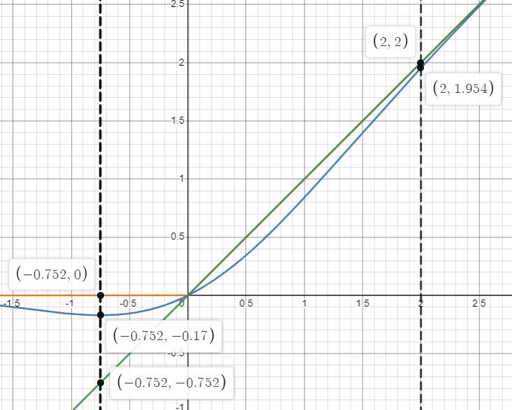
Figure 3: The black lines indicate the unactivated outputs of 2 neurons being considered for CAM. If Shift is introduced, the linear function gives the maximum difference between activated and unactivated neurons when compared to GeLU and ReLU. It also makes the sign of deactivated output irrelevant as the absolute function focuses more on the magnitude of the function.

The BERT architecture uses the GELU activation function for activating neurons but it is treated as a different module while pruning. Thus, the CAM outputs obtained are not activated. This results in the LayerGradCAM model performing significantly worse as seen in our SST-2 results 6. We then introduced the ReLU activation function which is very similar to the structure of the GELU activation function used in BERT. However, this causes many scores to become zero and results in the generation of erroneous masks. Thus, to ensure that CAM scores directly indicate the likelihood of a neuron being activated, we shifted all scores up by a scalar $\lambda$ which is a hyper-parameter. We believe this helped very clearly discern importance even among deactivated neurons thus giving a very good performance across our 3 datasets. For our experiments, we used a value of $10$ for $\lambda$.

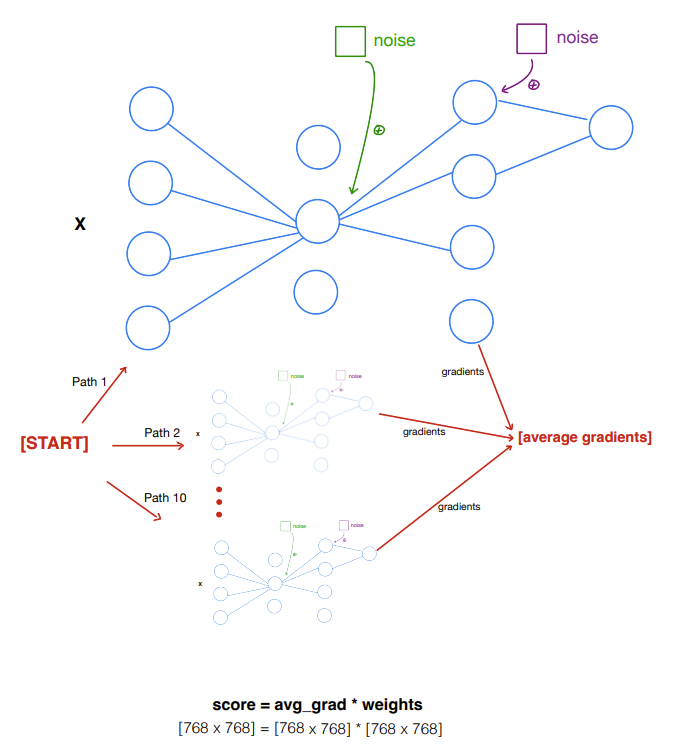
Figure 4: A depiction of smooth grad: Starting with an input vector, we add random noise samples from Gaussian distribution at each step of the forward process, and we do this for a total of 10 paths. The final gradient of the network for this input will be the average gradient across all the paths.

3.4.4 Final Scoring metric and Mask

Taking cumulative of all our ideas we thus derive the final scoring metric for LayerGradCAMShift as:

$$S=|w\times\frac{\partial{L}}{\partial{w}}\times(\frac{1}{l_{b}}\sum_{l_{b}}\frac{1}{l_{s}}\sum_{l_{s}}(w\cdot x+b)+\lambda)|$$ (5)

where $l_{s}$ is the sequence length, $l_{b}$ is the batch length, and $\lambda$ indicates the shift.

The final mask can be obtained like LayerMagWeight:

$$mask[w]=\begin{dcases*}1,&if $w\in$ top $q$ quantile of\\ &parameters in given tensor,\\ 0,&otherwise.\end{dcases*}$$ (6)

where $q$ is determined using the compression ratio and the number of prunable layers.

3.5 Smooth-Cut (LayerSmoothGrad)

3.5.1 Need for Smoothing

In interpretability literature, it was commonly observed that Vanilla Gradients or using only gradients provided noisy results thus normal noise was added to the input and the weighted sum of the gradients of noisy input was considered as a mask. The probability of the noise was considered as the weight thus making larger noise weigh less and smaller noise weigh more. This created a smoothing effect over the piecewise-linear manifold which provides a much better approximation of the gradients. This effect is clearly depicted in 5 Thus, we can formulate this in terms of weights, input, and biases as follows:

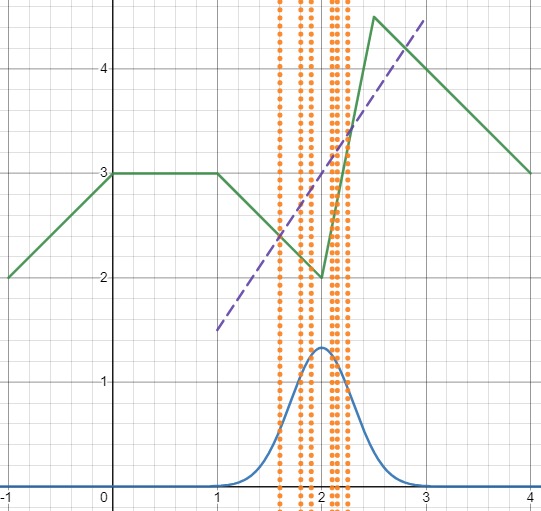
Figure 5: Smoothing Gradients of a piecewise linear function using sampling of noisy input

Let $z$ be a random variate sampled from a normal distribution with a variance of 0.01 and a mean of 0.

$$w_{noisy} =w+z$$ (7)

$$b_{noisy} =b+z$$

$$y_{noisy} =(w+z)\cdot x+(b+z)$$

$$=(w\cdot x+b)+z\cdot(1+x)$$

As the output of every layer is much smaller than $1$ in our observation we approximated this as:

$$y_{noisy}\approx(w\cdot x+b)+z$$ (8)

This is done using a forward hook in every layer and the $backward()$ function in $PyTorch$ is used to sample the gradient. For ease of implementation and as the variance in noise is small, we have taken a numeric average instead of the weighted average, unlike the SmoothGrad paper.

3.5.2 Implementation at scale

Ideally, every parameter tensor must be sampled with noise while keeping all other parameters constant to get a good estimate but this is not scalable with architecture as large as BERT. To overcome this limitation we instead reduce the variance in noise as it will be accumulated over multiple layers and add it in the forward pass at every layer. As the linear combination of Gaussian normal noise is also Gaussian, and the variance in noise is small we believe our method is able to sample the locality of weights very well. This thus gives a correlated noisy estimate of gradients for all parameters in every forward propagation. We thus sample $\eta$ such paths and average the gradients over all these paths giving a smoothed gradient approximation. As we sample $\eta$ different paths for every input, this method needs $\eta$ iterations for every sample whereas LayerGradCAMShift needs only $1$. To scale this approach to larger datasets, and fairly evaluate the two methods, we run all Smoothing methods with only 100 batches of gradients and each batch undergoes 10 smoothing operations denoted by $\eta$. This is clearly shown in 4.

3.5.3 Final Scoring metric and Mask

Taking cumulative of all our ideas we thus derive the final scoring metric for LayerSmoothGrad as:

$$S=|w\times\frac{1}{\eta}\sum_{i=1}^{i=\eta}\frac{\partial{L_{Noisy}}}{\partial{w}}|$$ (9)

The final mask can be obtained like LayerMagWeight:

$$mask[w]=\begin{dcases*}1,&if $w\in$ top $q$ quantile of\\ &parameters in given tensor,\\ 0,&otherwise.\end{dcases*}$$ (10)

where $q$ is determined using the compression ratio and the number of prunable parameters.

4 Evaluation

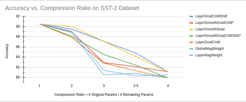
Figure 6: SST-2 dataset

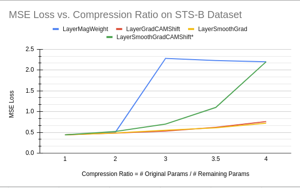
Figure 7: STS-B dataset

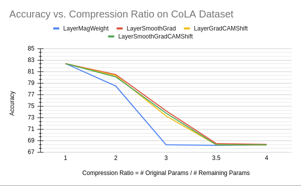
Figure 8: CoLA dataset

The main purpose of this evaluation is to check how much performance is retained for the given dataset and compression ratio, thus giving us deeper insights into the applicability and differences in our pruning methods.

To evaluate our pruning methods we test them over 3 datasets, SST-2, STS-B, and CoLA, and for $4$ compression ratios of $2,3,3.5,4$. We observed that there wasn’t much variation between ratios of $1$ and $2$, thus they were not run for all techniques.

The major questions we ask during evaluation are:

1. How much performance is lost for different compression ratios across different pruning strategies?

2. How important are parameters at various pruning thresholds thus giving an idea if performance behaves like the Pareto principle? 20% weights can give over $80\%$ of the expected results.

3. How different are the pruning masks generated by the various strategies and how do these differences turn out across different layers?

4.1 Dataset Details

The following GLUE datasets were used:

1. SST-2 (Stanford Sentiment Analysis Task): This has $67k$ training samples with 1.8k test samples. It allows only $2$ sentiment classes for classification.

2. STS-B (Semantic Textual Similarity Benchmark): This has $7k$ training samples with $1.4k$ test samples. It has a continuous target score ranging from $0$ to $5$ where $0$ indicates opposite sentences and $5$ equivalent sentences. This is a regression problem.

3. CoLA (Corpus of Linguistic Acceptability): This has $8.5k$ training samples and $1k$ testing samples. It tests if a sentence is grammatically acceptable or not and has a single sentence as input.

4.2 Evaluation Measures

We analyze the performance in terms of accuracy for SST-2 and CoLA and Mean Squared Error for the STS-B dataset and how it varies with increasing compression ratios in our datasets.

4.2.1 Evaluation Process

The pruning process involves a set of fine-tuning epochs which are followed by pruning and then re-fine-tuning. A batch size of $16$ with a learning rate of $1e-5$ and the Adam optimizer was used for SST-2 and CoLA datasets. For the STS-B dataset, we used a learning rate of $2e-5$. For the SST-$2$, dataset $3$ initial fine-tuning epochs were run and $8$ final fine-tuning epochs were used. For CoLA $5$ initial fine-tuning epochs and $12$ final-fine-tuning epochs were used. Finally, for the STS-B dataset, we used $8$ initial fine-tuning epochs and $10$ final-fine-tuning epochs. The models were finally chosen using early stopping and the learning rate, batch size, and the number of epochs were selected after observing the loss over multiple runs.

4.3 Results

We first present our results on the SST-2 Dataset in 6. Here we observe that we significantly outperform the baselines for all compression ratios. As can be observed, up to the compression ratio of $3$ LayerMagWeight outperforms GlobalMagWeight but both have similar performance after that. We also observe that Shift is essential for LayerGradCAM to perform well and the performance of LayerGradCAM is barely at the baseline possibly due to the weight signal. Another important observation is that even though LayerSmoothGrad and LayerGradCAMShift work well, their combinations LayerSmoothGradCAM and LayerSmoothGradCAMShift do not appear to perform equally well. We later identified that these combination methods were using gradients of only $1$ batch and thus do not seem to perform as well. We corrected this in CoLA and have provided the results.

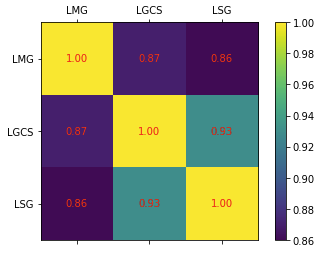
(a) Mean,Compression=3

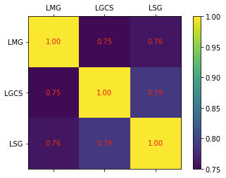
(b) Min,Compression=3

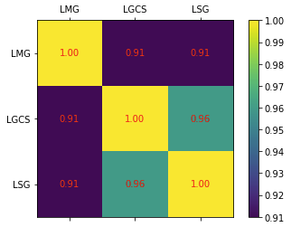
(c) Mean,Compression=3.5

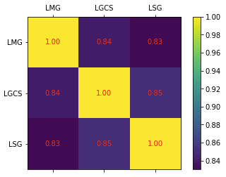
(d) Min,Compression=3.5

Figure 9: Here, 9a and 9b represent the confusion matrix of the mean and min values across all layers, respectively, for a compression ratio of 3. 9c and 9d represents the confusion matrix of the mean and min values across all layers, respectively, for a compression ratio of 3.5. LMG: LayerMagGrad, LGCS: LayerGradCAMShift, LSG: LayerSmoothGrad.

For the STS-B dataset in 7, the LayerGradCAMShift and LayerSmoothGrad methods perform extremely well incurring very low losses even at a compression ratio of $4$ whereas the LayerMagWeight baseline drastically loses its performance from a compression ratio of $3$ onwards.

For the CoLA dataset 8 we observe similar trends but possibly due to dataset specific reasons the performance flattens at $3.5$ compression at about $68.3$. In SST-2 and STS-B there was a much larger variation at compression ratios of $3.5$ and $4$ compared to CoLA.

Even at compression ratio $2$ across all datasets the performance is very similar irrespective of the pruning method used. At ratios of $3$ and $3.5$, the difference increases significantly and at the compression ratio of $4$, where less than $5\%$ of prunable parameters remain, we see the performance of all methods tending to converge at least for SST-2 and CoLA datasets in 6 and 8.

4.4 Analysis

As observed in our results the performance drops steeply with the compression ratio unless the method of pruning is suitable. Thus we conclude that it is essential to choose the right pruning strategy to get good results, especially for compression ratios greater than $2$. For all $3$ datasets, the performance at compression ratio $2$ varies marginally across all pruning strategies. We believe these results are due to the reason that many sub-networks can perform very well unless they are constrained to be too small. This is in accordance with Prasanna et al., (2020).

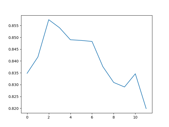
(a) Compression=3

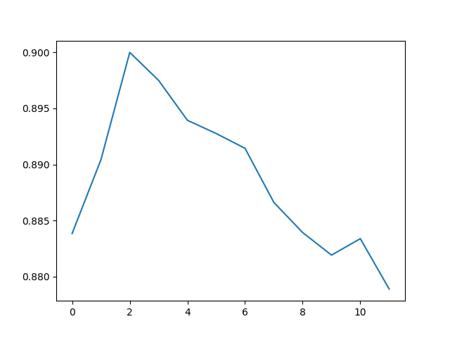
(b) Compression=3.5

Figure 10: Cam-Cut v/s LayerMagWeight attention-head IOUs at two different compression levels

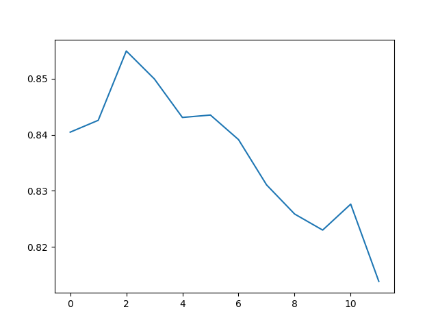
(a) Compression=3

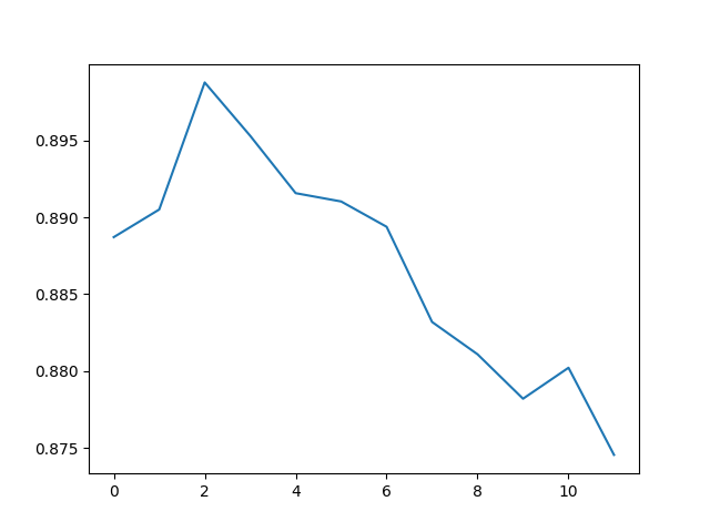
(b) Compression=3.5

Figure 11: Smooth-Cut v/s LayerMagWeight attention-head IOUs at two different compression levels

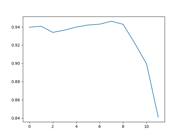
(a) Compression=3

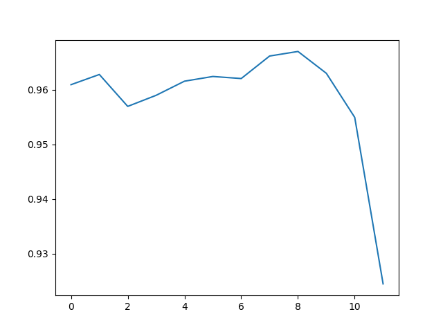
(b) Compression=3.5

Figure 12: Cam-Cut v/s Smooth-Cut attention-head IOUs at two different compression levels

Simultaneously we also observed that the weight information present in all our metrics is also very important. We did some experiments initially with compression ratios of $2$ without including the weight term and observed that the performance of the LayerGradCAM was not even surpassing the baseline. Thus we have included the weight term in all the strategies.

Beyond the compression ratio of $2$, we find that gradient information becomes extremely important. This is very evident as gradient-based methods easily surpass only weight-based ones. This is not seen until the compression ratio of $2$ and not even in some of our experiments with compression ratios of $1.5$.

Even in gradient-based methods, it is very important to have a gradient over a large significant portion of the dataset. Our runs using the combined methods LayerSmoothGradCAMShift and LayerSmoothGradCAM were initially taking gradients over only a single batch of 16 samples thus giving the degraded performances as seen in SST-2 and STS-B. But with many more batches, the performance improves significantly as seen in the CoLA dataset.

We also perform a detailed analysis of the masks created by the methods LayerMagWeight, LayerGradCAMShift, and LayerSmoothGrad for SST-2 dataset. We find the Jaccard distance of these masks which represents the intersection over the union of the weights which are selected after pruning at compression ratios of $3$ and $3.5$. We have computed the mean and min IOU across all layers for every pair of strategy as shown in 9. We can observe that the mean and min value of LayerMagWeight with both, Cam-Cut and Smooth-Cut is low, and the same values when we compare Cam-Cut and Smooth-Cut are high. This gives a hint at the similar and superior performance of both these strategies.

We further analyze these mask differences across layers of BERT as depicted in 10, 11, and 12. We find that LayerMagWeight has IOUs of about 82% to 86% across layers and this tends to drop as we go higher in the architecture irrespective of the strategy. As this trend is most pertinent with LayerMagWeight, it implies that the shallower and middle layers are the ones storing a lot of language modeling information in their weights and their weights are more important compared to gradients. On the other side, the higher weights seem more task-based, especially in the final layer where even LayerGradCAMShift and LayerSmoothGrad have more differences than others. Simultaneously, we also observe that LayerSmoothGrad and LayerGradCAMShift have very similar masks throughout various layers. On average they have about 95% similarity until the final layer of the model. This is a strong indicator that it is extremely likely that both models are converging to very similar sub-models despite having very different scoring metrics and structures. This is also probably the reason for both methods giving very similar performance. This also shares parallels with the interpretability literature where saliency masks are better if they are sparse and highlight the features of the region of interest. Every pixel highlighted must explain more variance in the output class than every pixel not highlighted. Similarly, every parameter selected must provide a greater gain in performance than every parameter removed.

5 Conclusion and Future Work

In this paper, we extended interpretability techniques to pruning and observed that many ideas developed to enhance interpretability transfer well to pruning. This also indicates that other interpretability works like DeepLIFT Shrikumar et al., (2017) can also be extended to further improve results. Our analysis also indicates that very different pruning metrics may end up converging to the same lottery ticket thus giving more insights into how different parameters play different roles in different downstream tasks. We also plan to analyze the similarity of pruning masks across different datasets and analyze differences in masks across layers of the BERT model. Finally, our insights in pruning metrics can translate into actual parameter reduction through structured iterative pruning in the future.

6 References

References

- tfp, (2019) (2019). Tensorflow pruning schematic. https://blog.tensorflow.org/2019/05/tf-model-optimization-toolkit-pruning-API.html.
- Blalock et al., (2020) Blalock, D., Gonzalez Ortiz, J. J., Frankle, J., and Guttag, J. (2020). What is the state of neural network pruning? Proceedings of machine learning and systems, 2:129–146.
- Cer et al., (2017) Cer, D., Diab, M., Agirre, E., Lopez-Gazpio, I., and Specia, L. (2017). Semeval-2017 task 1: Semantic textual similarity-multilingual and cross-lingual focused evaluation. arXiv preprint arXiv:1708.00055.
- Dai et al., (2021) Dai, D., Dong, L., Hao, Y., Sui, Z., and Wei, F. (2021). Knowledge neurons in pretrained transformers. arXiv preprint arXiv:2104.08696.
- Frankle and Carbin, (2018) Frankle, J. and Carbin, M. (2018). The lottery ticket hypothesis: Finding sparse, trainable neural networks. arXiv preprint arXiv:1803.03635.
- Gale et al., (2019) Gale, T., Elsen, E., and Hooker, S. (2019). The state of sparsity in deep neural networks. arXiv preprint arXiv:1902.09574.
- Han et al., (2015) Han, S., Mao, H., and Dally, W. J. (2015). A deep neural network compression pipeline: Pruning, quantization, huffman encoding. arXiv preprint arXiv:1510.00149, 10.
- Kurtic et al., (2022) Kurtic, E., Campos, D., Nguyen, T., Frantar, E., Kurtz, M., Fineran, B., Goin, M., and Alistarh, D. (2022). The optimal bert surgeon: Scalable and accurate second-order pruning for large language models. arXiv preprint arXiv:2203.07259.
- Lee et al., (2020) Lee, J., Park, S., Mo, S., Ahn, S., and Shin, J. (2020). Layer-adaptive sparsity for the magnitude-based pruning. arXiv preprint arXiv:2010.07611.
- Lee et al., (2018) Lee, N., Ajanthan, T., and Torr, P. H. (2018). Snip: Single-shot network pruning based on connection sensitivity. arXiv preprint arXiv:1810.02340.
- Louizos et al., (2017) Louizos, C., Welling, M., and Kingma, D. P. (2017). Learning sparse neural networks through regularization. arXiv preprint arXiv:1712.01312.
- Mahendran and Vedaldi, (2015) Mahendran, A. and Vedaldi, A. (2015). Understanding deep image representations by inverting them. In Proceedings of the IEEE conference on computer vision and pattern recognition, pages 5188–5196.
- Mishra et al., (2021) Mishra, A., Latorre, J. A., Pool, J., Stosic, D., Stosic, D., Venkatesh, G., Yu, C., and Micikevicius, P. (2021). Accelerating sparse deep neural networks. arXiv preprint arXiv:2104.08378.
- Ortiz et al., (2019) Ortiz, J. J. G., Blalock, D. W., and Guttag, J. V. (2019). Standardizing evaluation of neural network pruning. In Workshop on AI Systems at SOSP.
- Perez and Reinauer, (2022) Perez, I. and Reinauer, R. (2022). The topological bert: Transforming attention into topology for natural language processing. arXiv preprint arXiv:2206.15195.
- Prasanna et al., (2020) Prasanna, S., Rogers, A., and Rumshisky, A. (2020). When bert plays the lottery, all tickets are winning. arXiv preprint arXiv:2005.00561.
- Ribeiro et al., (2016) Ribeiro, M. T., Singh, S., and Guestrin, C. (2016). ” why should i trust you?” explaining the predictions of any classifier. In Proceedings of the 22nd ACM SIGKDD international conference on knowledge discovery and data mining, pages 1135–1144.
- Sanh et al., (2020) Sanh, V., Wolf, T., and Rush, A. (2020). Movement pruning: Adaptive sparsity by fine-tuning. Advances in Neural Information Processing Systems, 33:20378–20389.
- Selvaraju et al., (2017) Selvaraju, R. R., Cogswell, M., Das, A., Vedantam, R., Parikh, D., and Batra, D. (2017). Grad-cam: Visual explanations from deep networks via gradient-based localization. In Proceedings of the IEEE international conference on computer vision, pages 618–626.
- Shrikumar et al., (2017) Shrikumar, A., Greenside, P., and Kundaje, A. (2017). Learning important features through propagating activation differences. In International conference on machine learning, pages 3145–3153. PMLR.
- Simonyan et al., (2013) Simonyan, K., Vedaldi, A., and Zisserman, A. (2013). Deep inside convolutional networks: Visualising image classification models and saliency maps. arXiv preprint arXiv:1312.6034.
- Smilkov et al., (2017) Smilkov, D., Thorat, N., Kim, B., Viégas, F., and Wattenberg, M. (2017). Smoothgrad: removing noise by adding noise. arXiv preprint arXiv:1706.03825.
- Socher et al., (2013) Socher, R., Perelygin, A., Wu, J., Chuang, J., Manning, C. D., Ng, A. Y., and Potts, C. (2013). Recursive deep models for semantic compositionality over a sentiment treebank. In Proceedings of the 2013 conference on empirical methods in natural language processing, pages 1631–1642.
- Sundararajan et al., (2017) Sundararajan, M., Taly, A., and Yan, Q. (2017). Axiomatic attribution for deep networks. In International conference on machine learning, pages 3319–3328. PMLR.
- Voita et al., (2019) Voita, E., Talbot, D., Moiseev, F., Sennrich, R., and Titov, I. (2019). Analyzing multi-head self-attention: Specialized heads do the heavy lifting, the rest can be pruned. arXiv preprint arXiv:1905.09418.
- Wang et al., (2018) Wang, A., Singh, A., Michael, J., Hill, F., Levy, O., and Bowman, S. R. (2018). Glue: A multi-task benchmark and analysis platform for natural language understanding. arXiv preprint arXiv:1804.07461.
- Wang et al., (2017) Wang, H., Zhang, Q., Wang, Y., and Hu, H. (2017). Structured probabilistic pruning for convolutional neural network acceleration. arXiv preprint arXiv:1709.06994.
- Warstadt et al., (2018) Warstadt, A., Singh, A., and Bowman, S. R. (2018). Neural network acceptability judgments. arXiv preprint arXiv:1805.12471.
- Yang et al., (2021) Yang, Z., Zhang, A., and Sudjianto, A. (2021). Gami-net: An explainable neural network based on generalized additive models with structured interactions. Pattern Recognition, 120:108192.
- Yu et al., (2022) Yu, S., Yao, Z., Gholami, A., Dong, Z., Kim, S., Mahoney, M. W., and Keutzer, K. (2022). Hessian-aware pruning and optimal neural implant. In Proceedings of the IEEE/CVF Winter Conference on Applications of Computer Vision, pages 3880–3891.
- Zhang et al., (2021) Zhang, Z., Qi, F., Liu, Z., Liu, Q., and Sun, M. (2021). Know what you don’t need: Single-shot meta-pruning for attention heads. AI Open, 2:36–42.