Dynamics of Social Networks: Multi-agent Information Fusion, Anticipatory Decision Making and Polling

Social sensors are agents that provide information about their environment (state) to a social network after interaction with other social sensors – this information fusion is modeled by social learning. This paper surveys mathematical models, structural results and algorithms in controlled sensing with social learning in social networks.

Part 1, namely Bayesian Social Learning with Controlled Sensing, addresses the following questions: How does risk averse behaviour in social learning affect quickest change detection? How can information fusion be priced? How is the convergence rate of state estimation affected by social learning? The aim is to develop and extend structural results in stochastic control and Bayesian estimation to answer these questions. Such structural results yield fundamental bounds on the optimal performance, give insight into what parameters affect the optimal policies, and yield computationally efficient algorithms.

Part 2, namely, Multi-agent Information Fusion with Behavioral Economics Constraints, generalizes Part 1. The agents exhibit sophisticated decision making in a behavioral economics sense; namely the agents are rationally inattentive (exhibit limited attention span) and make anticipatory decisions (thus the decision strategies are time inconsistent and interpreted as subgame Bayesian Nash equilibria).

Part 3, namely Interactive Sensing in Large Networks, addresses the following questions: How to track the degree distribution of an infinite random graph with dynamics (via a stochastic approximation on a Hilbert space)? How can the infected degree distribution of a Markov modulated power law network and its mean field dynamics be tracked via Bayesian filtering given incomplete information obtained by sampling the network? How does the structure of the network (Erdős Rényi vs power law) affect estimation of the infected degree distribution and corresponding Cramer Rao bounds? We also briefly discuss how the glass ceiling effect emerges in social networks.

Part 4, namely Efficient Network Polling deals with polling in large scale social networks. In such networks, only a fraction of nodes can be polled to determine their decisions. Which nodes should be polled to achieve a statistically accurate estimate of sociological phenomena? Some nodes may be reluctant to reveal their true opinion. This may lead to incorrect polling estimates. How to compensate for this?

1 Introduction

This paper discusses controlled sensing and information fusion of interacting social sensors. In classical Bayesian signal processing, noisy observations recorded by physical sensors are used with Bayes rule to estimate an underlying state. Here we consider controlled sensing with social learning to estimate the underlying state. Social learning, or learning from the actions of others, is an integral part of human behavior and has been studied in behavioral economics, sociology and computer science to model the interaction of decision makers [14, 59, 19, 30, 2, 91, 48, 57, 93, 161, 186].

Social learning models present unique challenges from a statistical signal processing point of view. First, social sensors [50, 159] interact with and influence each other. For example, ratings posted on online reputation systems strongly influence the behavior of individuals. This is usually not the case with physical sensors. Second, due to privacy concerns and time-constraints, social sensors reveal decisions (ratings, votes) which are a quantized function of their raw measurements and interactions with other social sensors.

1.1 Background: What is Bayesian Social Learning? A Signal Processing Perspective

To fix ideas, we start with a short review of “vanilla” social learning. Let $\{x_{k}\}$ denote a finite state Markov chain with state space $\mathcal{X}=\{1,2,\ldots,X\}$, transition matrix $P$, and initial distribution $\pi_{0}$. Suppose at each time $k$, noisy measurements $y_{k}\in\mathcal{Y}$ are available, where $\mathcal{Y}$ is a finite set and $y_{k}$ is generated from conditional distribution $P(y_{k}=y|x_{k}=i)$. A multi-agent system aims to estimate the underlying state $x_{k}$, at each time $k$.

In classical Bayesian estimation, the multi-agent system has access to all previous observations. The posterior $\pi_{k}(i)=\mathbb{P}(x_{k}=i|y_{1},\ldots y_{k})$ is computed via the Hidden Markov model (HMM) filter [58, 60]
Classical HMM Filter $$\pi_{k+1}=T(\pi_{k},y_{k+1})\propto\underbrace{\mathbb{P}(y_{k+1}|x_{k+1}=j)}_{\text{likelihood}}\sum_{i}P_{ij}\,\underbrace{\pi_{k}(i)}_{\text{prior}}$$ (1)

In sequential social learning, agents do not have access to observations of other agents. Instead they only have access to the actions of previous agents. Each agent acts once in a predetermined sequential order indexed by $k=1,2,\ldots$. Let $a_{k}\in\{1,\ldots,A\}$ denote the action chosen by agent $k$. Then the posterior distribution (public belief) $\pi_{k}(i)=\mathbb{P}(x_{k}=i|a_{1},\ldots,a_{k})$ is updated via the following 3 step procedure [48]:
Social Learning Filter $\displaystyle\eta_{k+1}$ $\displaystyle=T(\pi_{k},y_{k+1})\quad\;\quad\text{agent updates private belief using HMM filter (\ref{eq:hmmfilter})}$ $\displaystyle a_{k+1}$ $\displaystyle=\operatornamewithlimits{argmin}_{a}c_{a}^{\prime}\eta_{k+1}\quad\text{agent takes action $a_{k+1}=\operatornamewithlimits{argmin}_{a}\mathbb{E}\{c(x_{k+1},a)|a_{1},\ldots,a_{k},y_{k+1}\}$}$ (2) $\displaystyle{\pi_{k+1}}$ $\displaystyle=S(\pi_{k},a_{k+1})\propto\underbrace{\sum_{y\in\mathbf{Y}}\mathbb{P}(a_{k+1}|y,\pi_{k})\,\mathbb{P}(y|x_{k+1}=j)}_{\text{likelihood}}\sum_{i}P_{ij}\,\underbrace{\pi_{k}(i)}_{\text{prior}}\quad\text{(public belief update)}$ (3)
Note that action $a_{k}$ in (2) is a quantized version of private belief $\eta_{k}$; this action is made public. The public belief $\pi_{k}$ computed by the social learning filter (3) is the posterior distribution given all actions until time $k$.

Key Point. The social learning filter (3) has a remarkable structure: the likelihood is an explicit function of the prior $\pi_{k}$; whereas in classical Bayesian filtering (1), the likelihood is functionally independent of the prior. This crucial difference results in unusual behaviour: herding, information cascades. Social learning is used to explain why customers choose crowded restaurants, and why financial booms and busts occur [48].

Perspective. Social learning originates in economics; yet it shares similarities with electrical engineering:

1. Social Learning vs Decentralized Detection. Decentralized detection (Tsitsiklis [179], Teneketzis [174], Varshney [185]) falls within the class of team decision theory [10] and shares many similarities to social learning but with key differences. Decentralized detection quantizes the observations, whereas social learning quantizes the Bayesian belief (2) leading to herd behavior and multi-threshold decision policies. In decentralized detection the fusion rules are directly optimized where as in social learning the fusion rule is prescribed (3).

2. Sequential Bayesian social learning. Part 1 considers controlled sensing assuming sequential interaction between agents in a Bayesian social learning framework. Even in this simple sequential setup there are several open issues regarding controlled sensing. Social learning has been extended to more general graphs [2, 3, 88, 92, 156, 1, 71, 133].

3. Decision-enabled sensor networks. The social learning framework also models decision enabled sensor networks where each individual node is a controlled sensor. A natural question is: How to control the interaction of autonomous decision makers as they learn from sensor data? Social learning with controlled sensing and fusion allows us to achieve coordination in decision making.

4. Real Datasets. Mathematical analysis alone cannot capture the complexity inherent in social sensing. See [68, 85, 84] for analysis on YouTube datasets. In [110, 74] we have studied herding and misinformation propagation amongst human subjects with experimental psychologists; see also [47].

1.2 Context – Three Interesting Examples

Controlled sensing with social learning can result in interesting behaviour (at least to a statistical signal processing audience). Here are three examples.

(i) Example 1. Change Detection with Social Learning can yield strange results: Consider the classical Bayesian quickest change detection problem: given noisy observations, detect if a change has occurred in the underlying state so as to minimize a linear combination of false alarm penalty and delay. It is well known [183, 163] that the quickest detection policy has a monotone threshold structure: when the posterior probability of change exceeds a threshold, it is optimal to declare a change. Therefore, the optimal stopping set (set of posteriors probabilities where it is optimal to declare “change”) is convex; see Figure 1(a).

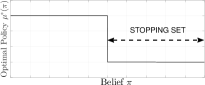
(a) Classical Quickest Detection has a convex (connected) stopping set

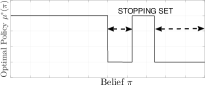
(b) Quickest Detection with social learning has a disconnected stopping set

Figure 1: Change detection. Classical vs social learning - these results are in our papers [98], [111].

Parts 1 and 2 generalize classical quickest detection to the case where social sensors interact via social learning (2), (3). Based on the local actions generated by social learning in (2), or equivalently, public belief $\pi$ computed by social learning filter (3), a global decision maker performs quickest change detection.

The optimal detection policy is shown in Fig.1(b). The remarkable feature is that the stopping set is disconnected. One sees in Fig.1(b) the counter-intuitive property: the optimal detection policy switches from announce “change” to announce “no change” as the posterior probability $\pi$ of a change increases!

Thus making a global decision as to whether a change has occurred based on local decisions of interacting agents is non-trivial. This has implications in anomaly/virality detection in social networks [160, 130] and detecting market shocks in economics [145],[105]. The result also has implications in automated sensing systems: be careful when quantizing Bayesian estimates (as in (2)) and then performing change detection.

The multi-threshold change detection policy is a form of change blindness: people fail to detect surprisingly large changes to scenes [164]. A human global decision maker might ignore the multi-threshold optimal policy and simply use the classical quickest detection policy. [102] shows that change-blindness is widely prevalent in anticipatory systems.

(ii) Example 2. Posterior Cramer Rao Bound (PCRLB) for social sensing – Power Law vs Erdős Rényi:

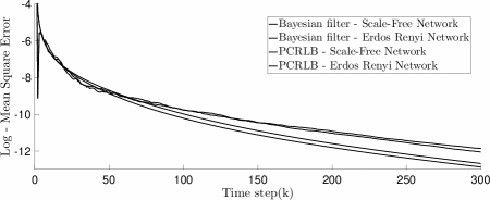
Figure 2: Mean square error and PCRLB for tracking infected degree distribution for Power law and Erdős-Rényi networks. Both PCRLB and its slope are insensitive to the underlying distribution [106].

Part 2 considers social sensors that interact on large graphs. We study optimal filtering to estimate information propagation (infected degree distribution) over time. A natural question is: How sensitive are the filtered estimates of the infected degree distribution to the underlying graph structure? Two important graph structures are the power law and Erdős Rényi networks. The power law network’s degree distribution decays polynomially as $k^{-\gamma}$, $k=0,1,\ldots$ and occurs in online social networks like Twitter. The classical Erdős Rényi network’s degree distribution decays exponentially as $e^{-\gamma k}$.

The PCRLB is a natural measure for the achievable performance of the mean square error of the filtered infected degree distribution estimate. Fig.2 compares the PCRLB for a power-law network versus an Erdős Rényi network. The surprising property in Fig. 2 is that both the PCRLB and its slope are insensitive to the underlying network structure. This suggests that for tracking the infected degree distribution, precise knowledge of the underlying network distribution is not required.

(iii) Glass Ceiling Effect in Social Networks

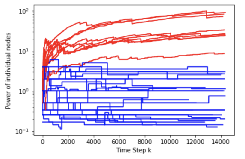
Figure 3: Simulated glass ceiling effect in a time evolving directed network (e.g. Twitter). The blue nodes constitute 80% of the population but their power never breaks through the glass ceiling. The power of a node is the ratio of number of followers to number of followees.

Here we illustrate a sociological dynamical effect in social networks that we will discuss in Part 3. The glass ceiling effect [17, 18] refers to the barrier that keeps certain groups from rising to influential positions, regardless of their qualifications. In analogy to real life, the glass ceiling effect is also highly visible in social networks such as Twitter, co-citation graphs and Instagram. In Twitter and Instagram, female users have a smaller following compared to their male colleagues who are equally qualified [172, 142]. A similar empirical observation is found in co-citation graphs where female authors receive less attention and fewer citations compared to their male colleagues and so are discouraged from academia [187, 86, 171]. Our recent work [138, 8] shows that during the global financial crisis in 2008, the glass ceiling effect on female authors was more pronounced; possibly due to more female authors being furloughed/laid off, or forced to change jobs. Our aim is to develop and analyze dynamic network models where individual nodes make decisions leading to a minority of nodes dominating high centrality positions in the network. This will shed light on the interplay between sociological phenomena such as perception bias [7], homophily [126] and the glass ceiling effect.

2 Part 1. Controlled Sensing with Social Learning – A POMDP Approach

The main ideas revolve around two extensions of the vanilla social learning protocol (2), (3):

1. Humans are often risk averse decision makers [176] whereas (2) specifies a social sensor as an expected utility maximizer. How is social learning affected when risk measures are used? Mathematically, a risk measure replaces the additive expectation operator in (2) with a subadditive risk operator. In engineering and economics, risk averseness models robustness; see page 2.2.3, and also the paper of economics Nobel laureate Sargent [75]. Since social learning is automated Bayesian decision making, Part 1 can be viewed as “robust controlled sensing amongst automated Bayesian decision makers.”

2. How does social learning interact with controlled sensing and controlled fusion? Social learning (2), (3) involves exchanging myopic decisions by social sensors to estimate an underlying state; while controlled sensing involves stochastic control over a time horizon to estimate an underlying state. This mismatch in time scales between myopic social sensors and a non-myopic controller (global decision maker) results in a non-standard controlled sensing problem.

2.1 POMDPs in Controlled Sensing: 4 Important Structural Results

Why? Partially observed Markov decision processes (POMDPs) are a natural framework for sequential Bayesian decision making under uncertainty. In this section we summarize new and potentially very widely applicable results for POMDPs that are of key importance in Part 1. These results apply to wide variety of problems including quickest change detection, controlled sensing, and controlled fusion with social learning.

Setup. Figure 4 displays our setup. The key point is the interaction between local decision makers (social sensors) and the global decision maker: in quickest change detection, the global decision to continue or stop determines whether social learning is continued; and as the local decisions accumulate via social learning, the global decision maker must decide when to declare a change. This yields a non-standard POMDP since the belief is updated using the social learning filter (3) instead of classical HMM filter (1). The optimal policy $\mu^{*}(\pi)$ satisfies Bellman’s dynamic programming equation, which involves the social learning filter:

$$\mu^{*}(\pi)=\operatornamewithlimits{argmin}_{u}Q(\pi,u),\;V(\pi)=\min_{u}Q(\pi,u),\text{ where }Q(\pi,u)=C(\pi,u)+\sum_{a}V\big{(}S(\pi,a,u)\big{)}\,\sigma(\pi,a,u).$$ (4)

Here $\pi$ is the posterior (belief state) computed via the social learning filter $S(\cdot)$ in (3); $C(\pi,u)$ is the cost incurred by the global decision maker for choosing action $u$ when the belief is $\pi$; and $V(\pi)$ is the value function. Recall $a_{k}$ is the action of the local decision maker which is available to the global decision maker.

Figure 4: Interaction of local decision makers (performing social learning) with a global decision maker that chooses decisions $u_{k}$ by solving a POMDP. We characterize the optimal policy in such controlled social sensing problems. The non-standard component compared to classical POMDPs is that the controller (global decision maker) only has access to previous local decisions $a_{k}$ and not private beliefs.

Why Structural results?: Although POMDPs are a useful modeling paradigm for controlled sensing, computing the optimal policy of a POMDP is in general intractable [144, 45, 123] since it requires solving Bellman’s equation (4) over the space of probability distributions (which is a continuum). We focus on structural results for the optimal policy rather than brute force numerical solutions. Structural results for POMDPs (studied in operations research, control theory and economics) yield bounds on the optimal performance, give insight into what parameters affect the optimal policies, and yield computationally efficient algorithms. They involve deep results in lattice programming and stochastic orders.

Below are four essential structural results for POMDPs (see [107, 108, 97, 98, 100, 111] and [122, 152, 153] for details).

Theorem 1 (Linear Cost Stopping Time POMDP [121]).

Consider a stopping time POMDP with two actions: $u=1\text{(stop)}$ and $u=2\text{ (continue)}$ with associated costs $C(\pi,u)$. If $C(\pi,u)$ is linear in the belief $\pi$ (as in standard POMDPs), then the stopping set $\mathcal{S}$, namely $\mathcal{S}=\{\pi:\mu^{*}(\pi)=1=\text{ stop}\}$ is a convex set.

Theorem 1 is well known. It is the reason why classical quickest detection (with geometric or more general phase-distributed change times) has a convex stopping region [97]. Unfortunately, to model risk in social learning, the cost $C(\pi,u)$ is non-linear in the belief $\pi$. Then the following novel generalization is required:

Theorem 2 (Threshold Optimal Policy for Non-linear Cost POMDP [97], [100]).

If the (possibly nonlinear) cost $C(\pi,u)$ is increasing wrt $\pi$ in terms of first order stochastic dominance, then under reasonable conditions on the transition and observation probabilities:

1. The stopping set $\mathcal{S}=\{\pi:\mu^{*}(\pi)=1=\text{ stop}\}$ is a connected set (but possibly non-convex).

2. The optimal policy $\mu^{*}(\pi)$ is increasing in $\pi$ with respect to the monotone likelihood ratio stochastic order. Therefore, $\mu^{*}(\pi)$ is characterized by a single threshold curve that partitions the belief space.

Figure 5: Threshold optimal policy for POMDP with nonlinear cost in $\pi$. The stopping set is connected

Theorem 2 was developed in [97, 100]. It applies to nonstandard quickest detection with nonlinear penalties in the belief; such as variance and exponential costs [97],[148]. The last sentence in Theorem 2 is the key point. Although computing the optimal policy via dynamic programming is intractable, Theorem 2 says that under suitable conditions the optimal policy is characterized by a single threshold curve; see Fig.5. One only needs to estimate this threshold curve! The optimal linear threshold policy which is increasing in $\pi$ can be computed straighforwardly via a simulation based stochastic gradient algorithm [115, 170]. Various parametrizations of the switching curve that result in a monotone policy can be obtained; such parametrized policies are optimal within the given parametric class.

Theorem 2 has two underlying concepts. First, we first need to order belief states (probability vectors). This is done using the monotone likelihood ratio order or its multivariate generalization called the TP2 (totally positive of order 2) order. Despite being partial orders, these are ideal for POMDPs since they are preserved under Bayesian updates.

The second, important concept to establish the threshold curve in Theorem 2 is a novel form of submodularity of Bellman’s equation (4); novel because it applies to specific line segments within the belief space. These line segments form chains, i.e., a totally ordered subsets for the likelihood ratio order. Submodularity implies $\mu^{*}(\pi)\uparrow\pi$ on each such chain; the union of such chains covers the belief space yielding the threshold curve.

The third result we outline below is tight myopic upper and lower bounds for the optimal policy of a POMDP.

Theorem 3 (Myopic Policy Bounds [111]).

Under copositivity conditions on the transition matrices, the optimal policy $\mu^{*}$ of a POMDP can be lower and upper bounded by myopic polices $\underline{\mu}$ and $\bar{\mu}$ so that

$$\underline{\mu}(\pi)\leq\mu^{*}(\pi)\leq\bar{\mu}(\pi),\quad\text{ for all beliefs $\pi$ }$$

Moreover, choosing the cots associated with the myopic policies $\underline{\mu}$ and $\bar{\mu}$ to maximize the region $\pi$ where $\underline{\mu}(\pi)=\bar{\mu}(\pi)$ can be formulated as a linear pogramming problem.

Under Blackwell dominance conditions [152] on the observation kernel (footnote 8), $\mu^{*}(\pi)$ can be upper bounded by a myopic policy. The tightest upper and lower bounds are obtained by solving a linear program.

Theorem 3 is useful for sub-optimal algorithms and establishing performance bounds in controlled sensing. They involve novel ideas in copositivity of stochastic matrices and Blackwell dominance [111, 100].

Finally, we present a performance analysis result. Can transition matrices $P$ and observation distributions $B$ be ordered so that the larger they are (with respect to a suitable partial order), the larger the optimal cumulative cost? Such a result is very useful – it allows us to compare the optimal performance of different POMDP social learning models, even though computing the optimal cost or policy is intractable.

Theorem 4 (Performance Analysis [99, 100]).

1. Consider two distinct POMDP models $\theta=(P,B)$ and $\bar{\theta}=(\bar{P},\bar{B})$, where $P\succeq\bar{P}$ wrt copositive dominance and $B\succeq\bar{B}$ wrt Blackwell dominance. Then under reasonable conditions, the optimal costs satisfy $J_{\mu^{*}(\theta)}(\pi;\theta)\leq J_{\mu^{*}(\bar{\theta})}(\pi;\bar{\theta}).$

2. Consider two distinct POMDPs $\theta=(P,B)$ and $\bar{\theta}=(\bar{P},\bar{B})$. Then for mis-specified model and mis-specified policy, the following sensitivity bounds hold (where constant $K$ can be determined explicitly)

   Mis-specified Model: $$\sup_{\pi\in\Pi}|J_{\mu^{*}(\theta)}(\pi;\theta)-J_{\mu^{*}(\theta)}(\pi;\bar{\theta})|\leq K\|\theta-\bar{\theta}\|.$$ (5)

   Mis-specified policy: $$J_{\mu^{*}(\bar{\theta})}(\pi,\theta)\leq J_{\mu^{*}(\theta)}(\pi,\theta)+K\|\theta-\bar{\theta}\|.$$ (6)

Note that (6) is a lower bound for the cumulative cost of applying the optimal policy for a different model $\bar{\theta}$ to the true model $\theta$ - this bound is in terms of the cumulative cost of the optimal policy for true model $\bar{\theta}$. So if the “distance” between the two models $\theta,\bar{\theta}$ is small, then the performance loss is small (5), (6).

2.2 Quickest Change Detection with Risk Averse Social Sensors

Quickest detection is a simple example of a stopping time POMDP and serves as a useful example. Recall the applications in virality detection and market shocks listed on page 2. (Quickest detection with measurement cost [20], quickest transient detection [150], quickest state detection are other important examples; see [97, 100] for formulation as a stopping time POMDP.)

In classical Bayesian quickest detection, the aim is to determine the optimal policy $\mu^{*}$ to minimize the Kolmogorov–Shiryaev criterion [149, 163, 183, 173] which is a tradeoff between delay and false alarm penalty:

$$J_{\mu}(\pi_{0})=d\,\mathbb{E}_{\mu}\{(\tau-\tau^{0})^{+}|\pi_{0}\}+f\,\mathbb{E}_{\mu}\{I(\tau<\tau^{0})|\pi_{0}\}.$$ (7)

Here $\tau_{0}$ is the change time, $\tau$ is the time when the detector announces a change has occurred, $d$ and $f$ denote the delay and false alarm penalties, respectively. Classical quickest detection is a linear cost stopping time POMDP. Therefore, Theorem 1 immediately implies that the optimal detection policy $\mu^{*}(\pi)$ has a threshold structure in the belief $\pi$ (see Fig.1(a)); where $\pi$ is computed by the HMM filter (1).

Standard quickest detection (17) is expectation centric. We consider two generalizations:

1. Decision makers influence each other via the social learning protocol (2), (3). (In signal processing, physical sensors usually do not affect each other.) So the belief $\pi$ is computed via social learning (3).

2. Social sensors are risk averse. So the expectation operator $\mathbb{E}$ in social learning (2) and $\mathbb{E}_{\mu}$ in controlled sensing (17) are replaced by coherent risk measures [11, 12]; thereby modeling risk averse local and global decision makers. It is well documented in behavioral economics [52, 55] that humans prefer a certain outcome over an uncertain but potentially larger outcome. To model risk averse behaviour, widely used coherent risk measures are Conditional Value-at-Risk (CVaR) [154, 155], Entropic/exponential risk measure [89] and Tail value at risk [129]; see also page 2.2.3 for robustness interpretation of risk in terms of dynamic risk measures for the global decision maker.

2.2.1 Why does Quickest Detection with Social Learning yield Strange Results?

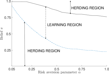
Figure 6: Effect of risk averse behavior on social learning [105]. The figure shows the regions in belief space where social learning and herding occur. When social sensors are more risk averse ($\alpha\rightarrow 0$), then the herding region becomes larger. Social sensors stick to the decision of previous sensors thereby exhibiting safety in numbers.

Consider the generalization of classical quickest detection where a multiagent system performs social learning [98, 105, 100]. Given the public belief $\pi$ computed by the social learning filter (3), the global decision maker’s policy $\mu^{*}:\pi\rightarrow\{\text{stop},\text{ continue}\}$ that optimizes the quickest detection objective (17) satisfies Bellman’s dynamic programming equation for a stopping time POMDP; see (4) for notation: $\mu^{*}(\pi)=\operatornamewithlimits{argmin}\{\}$,

$$V(\pi) =\min\{f\pi(2),\;d(1-\pi(2))+\sum_{a\in\mathbb{A}}V\left(S(\pi,a)\right)\sigma(\pi,a)\}.$$ (8)

As discussed on page 1.2, the remarkable result regarding Bellman’s equation (8) is that the optimal policy is multi-threshold as shown in Fig.1(b). This means that the optimal policy switches to “no change” as the probability of change becomes larger! Also the value function $V(\pi)$ is non-concave. This is very different to a classical quickest detection where the policy is monotone (threshold) and the value function is concave.

Unusual structure of social learning filter. In a nutshell, the above unusual multi-threshold behavior is due to the unusual structure of the social learning filter $S(\pi,a)$ in (8). For $P=I$, the social learning filter (3) has two distinct behaviors depending on the prior belief $\pi$ [98, 100]:

1. For $\pi$ in the herding region, $S(\pi,a)=\pi$. So the agent simply repeats the action of the previous agent.

2. In the learning region, $S(\pi,a)=T(\pi,y)$, i.e., the social learning filter (3) coincides with the classical Bayesian update (1). The size of the herding and learning regions depend on the costs $c(x,a)$ in (2).

As a result, of this discontinuity, for two beliefs $\pi_{1},\pi_{2}$ which are very close, the updates can be vastly different. This results in a non-concave value function $V$ in (8) and hence, a multi-threshold optimal policy.

2.2.2 Quickest Detection with Risk Averse Social Learning

Next, consider the further generalization where expectation centric social learning is replaced with risk averse social learning, i.e., risk averse local decision makers. To save space, we focus on the CVaR risk measure; however, our research will study general risk averse measures. In analogy to social learning (2), given observation $y_{k}$, the local decision maker chooses action $a_{k}$ at time $k$ to minimize the CVaR cost:

$$a_{k}={\underset{a}{\text{argmin}}}\{\text{CVaR}_{\alpha}(c(x_{k},a))\}={\underset{a}{\text{argmin}}}\{{\underset{z\in\mathbb{R}}{\text{min}}}~{}\{z+\frac{1}{\alpha}\mathbb{E}_{y_{k}}[{\max}\{(c(x_{k},a)-z),0\}]\}\}.$$ (9)

Here $\alpha\in(0,1]$ is the degree of risk-aversion for the agent (smaller $\alpha$ implies more risk-averse behavior). (9) together with (3) constitutes the CVaR social learning filter.

Q1. What are the structural properties of the risk averse social learning filter? [110] shows that, under reasonable assumptions on the costs, the decisions taken by risk-averse agents are ordinal functions of their private observations and monotone in the prior information. Thus Bayesian social learning follows simple intuitive rules and is a useful idealization of human behavior; see the highly influential paper [127]. Fig.6 shows the herding regions in the belief space for CVaR risk averse social learning filter. It can be observed from Fig.6 that the region of beliefs where social learning occurs grows smaller as the parameter $\alpha$ decreases (agents become more risk averse). So Fig. 6 can be interpreted as saying that risk-averse agents show a larger tendency to go with the crowd rather than “risk” choosing the other action. In particular as $\alpha\rightarrow 0$ (extreme risk averse case), the entire state space becomes a herding region.

Q2. How is Quickest Change Detection Policy affected by risk averse social sensors? [105] shows numerically that the stopping region is non-convex. Our objective is to characterize the optimal policy (extensions of Theorems 2, 3, and 4).

Interpretation: Multi-threshold behavior reflects the lack of confidence by the global decision maker: if it is optimal to announce a change, it may not be optimal to declare a change when the belief is higher. So the above conjecture says: If the decision maker is confident of announcing a change for a certain risk aversion, then it remains confident of its decision when the agents are more risk averse (more careful). Another interpretation is in terms of change blindness as discussed in the Introduction.

Q3. Optimal Achievable Cost? The risk averse behavior in social learning manifests itself in the action likelihood (3). This likelihood is the product of the classical likelihood matrix with a conditional probability. We will use Blackwell dominance in Theorem 4 to show that the cost incurred by quickest detection with risk averse social learning is always larger than classical quickest detection. Also Theorem 3 yields myopic bounds that sandwich the optimal policy and upper bounds to the achievable cost.

2.2.3 Robust Quickest Detection with social learning using dynamic risk measures

Thus far, we have considered quickest detection where risk averse local decision makers that perform social learning. Now we consider a risk averse global decision maker that performs quickest change detection. Since the global decision maker solves a POMDP, we need to use dynamic risk measures.

Why? Dynamic risk averse measures model robustness in decision making. Let us quickly explain this. The Kolmogorov-Shiryaev criterion (17) for quickest detection optimizes the additive objective $\mathbb{E}_{\mu}\{J\}$ wrt policy $\mu$, where $J$ is the accumulated sample path cost. In risk averse control with an exponential penalty, one seeks to optimize $J_{R}=\mathbb{E}_{\mu}\{\theta\exp(\theta J)\}$ where $\theta>0$ denotes the risk averse parameter. Expanding the exponential yields $J_{R}=\theta+\theta^{2}\mathbb{E}_{\mu}\{J\}+\theta^{3}c_{\theta}\mathbb{E}_{\mu}\{J^{2}\}$ for some constant $c_{\theta}$. So $J_{R}$ penalizes heavily large sample path costs due to the presence of second order moments and therefore is used widely in robust control [188, 147, 26, 75]. Interestingly, [148] published in 1998 is the first exponential risk quickest detection paper. Of course, today the exponential penalty is just one of a large number of risk averse measures. In particular, with the rapid recent progress in coherent risk measures (see footnote 6), there is strong motivation to develop robust controlled sensing results; see also [180] for minimax robustness.

How? Risk averse control replaces the expectations $\mathbb{E}_{\boldsymbol{\mu}}\{\cdot|\pi_{0}\}$ in stochastic control by more general subadditive dynamic risk measures. Accordingly, consider the global decision maker’s risk averse objective

$$J_{\boldsymbol{\mu}}(\pi_{0})=\mathbf{R}^{0}_{\boldsymbol{\mu}}\biggl{\{}c(x_{0},u_{0})+\mathbf{R}^{1}_{\boldsymbol{\mu}}\bigl{\{}c(x_{1},u_{1})+\cdots+\mathbf{R}^{N-1}_{\boldsymbol{\mu}}\{c(x_{N-1},u_{N-1})+c_{N}(x_{N})\}\bigr{\}}|\pi_{0}\biggr{\}}.$$ (10)

Here, the one step risk measures $\mathbf{R}^{0}_{\boldsymbol{\mu}},\mathbf{R}^{1}_{\boldsymbol{\mu}},\ldots$ replace the expectation operator $\mathbb{E}_{\boldsymbol{\mu}}$ in (17). The operators $\mathbf{R}^{k}_{\boldsymbol{\mu}}\big{\{}\phi(x_{k},u_{k},x_{k+1})\big{\}}$ are called Markov risk transition mappings and are a sub-additive generalization of the conditional expectation $\mathbb{E}\{\cdot|x_{k},u_{k}\}$, see [158, 46] for detailed exposition of dynamic risk measures.

Bellman’s equation for quickest detection with dynamic CVaR risk and social learning reads (recall from (9) that $\alpha\in(0,1]$ models the degree of risk-aversion): optimal policy $\mu^{*}(\pi)=\operatornamewithlimits{argmin}\{\cdot\}$ and

$$V(\pi)=\min\{f\,\pi(2),d\,(1-\pi(2))+\inf_{z\in{\rm IR}}\big{\{}z+\frac{1}{\alpha}\sum_{y}\max\{V(S(\pi,a))-z,0\}\sigma(\pi,a)\}.$$ (11)

Notice the substantial difference compared to the risk neutral Bellman’s equation (8) for quickest detection. In the most general setup we will consider: individual social sensors are risk averse in their decision making, and a dynamic risk measure is used in the control objective for the global decision maker. We can constrict structural results for the optimal policy by extending Theorem 2, see [100, 105]. Using Theorem 3 we can construct myopic policies that provably upper and lower bound the optimal policy. This allow us to determine achievable bounds to the optimal cost (see Theorem 4).

2.3 Controlled Information Fusion with Social Sensors

Thus far, the interaction of global and local decision makers was limited to controlling the local decisions over time. We now consider controlled social learning. We wish to determine How to price the quality of local decisions over time, to achieve controlled information fusion?

In the classical social learning protocol (2), (3), social sensors are interested in minimizing their own myopic costs (2) and ignore the information benefits their action provides to others. This leads to an information cascade and social learning stops (when estimating a random variable). Our aim is to devise algorithms to delay herding until the state estimate has reached acceptable accuracy. Below we discuss how the global decision maker can affect the quality of the observations (actions) amongst the social sensors in three ways:

1. Controlling the information structure (Sec.2.3.1)

2. Pricing information fusion (Sec.2.3.2)

These constitute socialistic learning: agents coordinate their actions to achieve a common goal.

2.3.1 Controlling the Information Structure in Social Learning – Privacy vs Reputation

Why? Controlling the information structure is important in adaptive trust/reputation social systems [96, 134]. Can social sensors assist social learning by choosing their actions to trade off individual privacy (local costs) while optimizing the reputation of their social group (global cost)? Building on [98, 99], agents minimize the welfare cost involving all agents $k=1,2,\ldots$ in their group (compared to myopic objective (2)):

$$J_{\mu}(\pi_{0})=\mathbb{E}_{\mu}\biggl{\{}\sum_{k=1}^{\infty}\rho^{k-1}c(x,a_{k})|\pi_{0}\biggr{\}},\;\text{ subject to privacy constrained rule }a_{k}=a(\pi_{k-1},y_{k},\mu(\pi_{k-1})).$$ (12)

The key point in (12) is that each agent chooses its action according to the privacy constrained rule [48, 168]. The strategy $\mu:\pi_{k-1}\rightarrow\{1,2\ldots,L\}$ maps the available public belief to the set of $L$ privacy values. The higher the privacy value, the less the agent reveals through its action. This is in contrast to classical social learning (2) where the action $a(\pi,y)$ is chosen as a myopic function of the observation and public belief.

How? Quickest Herding optimal policy. The optimal policy $\mu^{*}(\pi)$ that minimizes (12) satisfies Bellman’s equation (4).

To gain insight, suppose there are two privacy values and each agent $k$ chooses action

$$a_{k}=\begin{cases}y_{k}&\text{ if }\mu(\pi_{k})=1\text{ (no privacy)}\\ \arg\min_{a}c_{a}^{\prime}\pi_{k-1}&\text{ if }\mu(\pi_{k})=2\text{ (full privacy)}.\end{cases}$$

So an agent either reveals its observation (no privacy) or chooses its action by neglecting its observation (full privacy). Notice that once an agent chooses full privacy, then all subsequent agents choose the same action and therefore herd - this follows since each agent’s action reveals nothing about the underlying state. Therefore, the problem is a stopping time POMDP: Determine the earliest time for agents to herd (maintain full privacy) subject to maximizing the social group reputation. We have the following results:

• The classical Theorem 1 does not apply since the costs $\operatornamewithlimits{argmin}_{a}c_{a}^{\prime}\pi$ are non-linear in belief $\pi$.

• But Theorem 2 from our previous work [97, 100] does apply! It says that the optimal policy $\mu^{*}$ has a threshold structure. Indeed the stopping set is non-convex but connected!

• If individuals deploy the heuristic “Choose increased privacy when belief is close to the target state,” then group behavior is sophisticated: herding is delayed and accurate state estimates are obtained.

How can the quickest herding results be extended to risk averse agents and dynamic risk measures? As in Theorem 2, the stopping region is connected but non-convex. This is in stark contrast to the results of the previous section where the stopping region is the union of disconnected sets. With Theorem 3, the optimal policy can be sandwiched by myopic lower and upper bounds; and the region where these bounds overlap can be optimized via a linear program.

2.3.2 Optimal Pricing of Information Fusion in Social Learning Framework

We next turn to controlling fusion by pricing information; which is important in automated decision systems [33]. Suppose a fusion center pays social sensors to choose actions that help the fusion center estimate the underlying state. For $k=1,2,\ldots$, let $p_{k}$ denote the price paid to social sensor $k$ to choose an action that reveals its private observation $y_{k}$. So the cumulative payment (cost) accrued by the fusion center is

$$J_{\mu}(\pi)=\mathbb{E}_{\mu}\{\sum_{k=1}^{\infty}\rho^{k-1}p_{k}\,I(a_{k}=y_{k})\mid\pi_{0}=\pi\},\quad\text{ where }p_{k}=\mu(\pi_{k-1}).$$ (13)

Here $\pi_{k}$ is the belief state computed via the social learning protocol (3). How can the fusion center minimize its cumulative payment (13) while simultaneously maximizing the accuracy of the state estimate?

[29] reveals two interesting results:

1. The optimal price sequence is a supermartingale, that is, $\mathbb{E}\{p_{k+1}|a_{1},\ldots,a_{k}\}\leq p_{k}$ implying that $\mathbb{E}\{p_{k+1}\}\leq\mathbb{E}\{p_{k}\}$. That is, on the average, it is always better to pay agents more to obtain more accurate estimates initially, and subsequently, as the state estimate gets more accurate, pay less.

2. The optimal pricing policy $\mu^{*}(\pi)$ has a piecewise monotone structure in the belief state $\pi$. This follows from Theorem 2.

Monopolist Interpretation.

The above result has a useful parallel in economic pricing [48] that we will explore and generalize. Suppose instead of $I(a_{k}=y_{k})$ in (13) one uses $I(a_{k}=1)$ which denotes a customer buying a product from a monopolist at price $p_{k}$. Each time a customer buys from the monopoly, two things happen: the monopoly makes money due to the sale; also its gets publicity via social learning (review on social media). The monopolist chooses its price $p_{k}=\mu(\pi_{k-1})$ based on the public belief $\pi_{k-1}$ to maximize its cumulative discounted reward. The optimal price is again a supermartingale [48]: so $\mathbb{E}\{p_{k+1}\}\leq\mathbb{E}\{p_{k}\}$.

Summary

Part 1 dealt with Bayesian estimation and controlled sensing/fusion involving sequential social learning. The main ideas involved structural results (stochastic orders and lattice programming) for risk averse controlled sensing of social sensors and pricing information fusion in POMDPs.

3 Part 2. Multi-agent Information Fusion. Behavioral Economics Constraints

We now discuss multi-agent information fusion with behavioral economics constraints. This is a substantial generalization of classical data fusion. In classical data fusion, a fusion center combines estimates from physical sensors to estimate an underlying state. Even in its classical form, information fusion with social sensors is challenging due to inefficiencies in social learning [30, 19, 48, 47, 131, 193] such as herding and information cascades, i.e. , agents ignore their own observations and parrot decisions of previous agents. Moreover, having more social sensors is not always advantageous (in reducing mean square error) – crowds can be more biased than individuals.

Part 2 generalizes Part 1 as we consider multi-agent information fusion when individual agents are sophisticated decision makers in a behavioral economics sense - they exhibit rational inattention and are anticipatory. Unfortunately, classical social learning is too simplistic to model the peculiarities of human decision making. Adding behavioral economics constraints to social sensors presents unique challenges from a statistical signal processing point of view. First, agents have limited attention spans. According to the paradigm of rational inattention, attention is a time-limited resource that can be modeled in terms of an information-theoretic (Shannon) channel capacity. In statistical signal processing terms, rational inattention is a form of controlled sensing: obtaining a more accurate observation requires more attention by the social sensor and therefore costs more.

Second, agents are anticipatory: they make decisions by taking into account the probability of future decisions (plans). In anticipatory decision making, the dependence of the current reward on future plans results in a deviation between planning and execution. This phenomenon is called time-inconsistency [31] and Bellman’s principle of optimality no longer holds. The appropriate formalism is the subgame Nash equilibrium. In game-theoretic terms, time-inconsistency arises when the optimal policy to the current multi-stage decision problem is sub-game imperfect. Anticipatory decision making is studied extensively in behavioral economics [43, 35] because it mimics important features of human decision making. Studies in psychology, neuroscience [22, 49, 36, 35] indicate that humans are anticipation-driven, and even simple decisions involve multi-stage planning. Time inconsistency of anticipatory decision making results in the planning fallacy of Kahneman & Tversky [90]: people tend to be optimistic and underestimate the time required to complete a future task. It is therefore important to incorporate behavioral economics constraints to model and analyze interacting social sensors.

Remark. The reader may be familiar with risk-sensitive/averse stochastic control [89, 65]. Traditionally, risk aversion is a static concept whereas anticipatory decision making involves a multi-stage setting. For example, CVaR (conditional value-at-risk [154, 155]) is a static coherent risk measure. This distinction blurs in more general dynamic risk formulations [158, 46], but then the clarity and elegant structure of human anticipatory decision making is lost; see also [105, 104].

Background. Anticipatory Agents, Rational Inattention, Time Inconsistent Decision Making

Anticipatory decision making and rational inattention are two important behavioral economics models; we briefly discuss them in a simplified mathematical sense to explain our ideas.

Anticipatory Decision Making. The key idea behind the anticipatory decision model [43] is as follows: Let $s_{1},s_{2}$ denote an underlying state at times 1,2. Then an anticipatory agent chooses decisions $a_{1},a_{2}$ from strategies $\mu_{1},\mu_{2}$ to maximize a 2-stage utility ([35] has a general multi-stage formulation)

$$\sup_{\mu_{1},\mu_{2}}J(s_{1},{\mu_{1},\mu_{2}}) =\sup_{\mu_{1},\mu_{2}}\mathbb{E}_{\mu_{1},\mu_{2}}\{r_{1}(s_{1},a_{1},\underbrace{\{p(a_{2}=a|s_{1},a_{1},\mu_{2}),a\in A\}}_{\text{anticipatory term}})+r_{2}(s_{2},a_{2})\}$$ (14)

The 2-stage utility (14) looks just like a standard time separable utility for a Markov decision process, except for the anticipatory term $\{p(a_{2}=a|s_{1},a_{1},\mu_{2}),a\in{A}\}$ in the reward $r_{1}$; this models anxiety (psychological state) of the decision maker. The dependency of the reward at time 1 on the probability of future actions (at time 2) results in time inconsistent decision making; Bellman’s principle of optimality does not hold [4, 31].

The time inconsistent decision problem (14) is ‘solved’ using the so called extended Bellman equation [43, 31] to obtain the subgame perfect Nash equilibrium strategies

$$\mu_{2}^{*}(s_{2})=\operatornamewithlimits{argmax}_{a_{2}}r_{2}(s_{2},a_{2}),\quad\mu_{1}^{*}(s_{1})=\operatornamewithlimits{argmax}_{a_{1}}J(s_{1},a_{1},\mu_{2}^{*})$$ (15)

For time inconsistent problems, neither the Nash equilibrium $\mu_{1}^{*},\mu_{2}^{*}$ nor its value $J$ are unique [31]. This is in contrast to classical dynamic programming where the optimal value is always unique. Note that the subgame Nash equilibrium approach to time inconsistency disregards the fact that $\mu_{2}^{*}$ is no longer optimal at time 1. Another insightful way of viewing this is that the estimated anticipatory reward $r_{1}(\cdot)$ requires the agent to extrapolate what might happen at the second stage, plans are not optimal once an action is taken [31].

Obviously humans do not solve time inconsistent problems to make decisions; even professors struggle with such formalisms! Time inconsistent behavioral economics models are widely used because they provide generative models for the peculiarities of human decision making. Indeed [43] shows that the above simple two-stage model captures important aspects of time-inconsistent human decision making:

1. Anticipatory agents act to reduce anxiety. [53] presents experimental results where people chose a more painful electric shock today than waiting anxiously for a less painful shock tomorrow.

2. Anticipatory agents deliberately avoid information by ‘sticking their head in the sand’ (with obvious consequences in decision making). [128] reports that giving patients more information of a medical surgery procedure raised their anxiety and decreased their probability of choosing the correct decision.

Multi-agent Rational Inattention. Finally a few words about rational inattention Sims [165, 166]. To quote Sims “Rational inattention models introduce the idea that people’s abilities to translate external data into action are constrained by a finite Shannon capacity to process information”.

A multi-agent rational inattention Bayesian model has the following dynamics [44, 41, 162, 42]: Given decisions $a_{1},\ldots,a_{k-1}$ of previous agents, agent $k$ chooses its observation $y_{k}$ with attention span $u_{k}$ and then makes decision $a_{k}$ via the following two-stage optimization (where cost $c$ depends on an underlying state $x$)

$$\begin{split}(u_{k},a_{k})&=\operatornamewithlimits{argmin}_{u}\mathbb{E}_{y}\big{\{}\operatornamewithlimits{argmin}_{a}\underbrace{\mathbb{E}\{c(x,a)|a_{1:k-1},y_{k},u\}}_{\text{expected cost}}+\lambda\big{[}\underbrace{H({\pi})-H({T(\pi,y,u)})}_{\text{ {rational inattention cost}}}\big{]}\big{\}}\end{split}$$ (16)

Here $\pi$ is the prior, and $T(\pi,y,u)$ denotes the Bayesian posterior given observation $y$ and attention $u$. Also $\lambda$ is a positive constant and $H(\pi)=-\sum_{i=1}^{X}\pi(i)\log_{2}\pi(i)$ is the Shannon entropy.

The mutual information between the prior and posterior, namely, $H(\pi)-H(T(\pi,y,u))$ in (16), is called the information acquisition cost in behavioral economics. Clearly, choosing a higher attention span yields a more accurate observation $y$ of state $x$ and reduces uncertainty in the updated belief $T(\pi,y,u)$; so the entropy $H(T(\pi,y,u))$ becomes smaller. Thus, the information acquisition cost becomes larger. So rational inattention (16) trades off observation accuracy with information acquisition cost.

Obviously humans do not solve a Bayesian optimization with entropy cost to make decisions! Rational inattention it is a useful generative model. Experimental studies [165, 166, 44, 41] show that human decision making is consistent with rational inattention. Our recent work [84] analyzes a massive YouTube data set and shows that the commenting behavior of users is consistent with rational inattention; indeed these models yield remarkably accurate predictive performance.

3.1 Multi-agent Quickest Detection with Anticipatory Decision Makers

With the above background, we now discuss multi-agent quickest detection. We study quickest detection since it serves as a launching pad for understanding more general stochastic stopping time problems involving interacting social agents; see [100, 105, 102].

Classical quickest detection deals with detecting a change in an underlying state given noisy observations. We consider the following generalization: How to detect a change in the strategy of rationally-inattentive anticipatory agents when they interact over a social network? The reader should keep in mind the following motivating example. Consider a social media accommodation system such as Airbnb [62]. By observing the reservation decisions of customers, how can Airbnb detect if there is a sudden change in the demand for a specific accommodation (apartment) due to the presence of a new competitor or change in quality of the existing accommodation? [102] contains several results. Unlike classical quickest detection, we only have access to the actions of the agents from their sub-game Nash equilibrium (15). As a result, the Bayesian belief (posterior) update structure is much more complex than classical quickest detection. This causes remarkably counter-intuitive behavior as we will investigate below.

Quickest detection aims to determine the optimal stopping time policy $\mu^{*}$ to minimize a cumulative cost involving false alarm and delay called the Kolmogorov–Shiryaev criterion of disorder [149, 163, 183, 173]:

$$\inf_{\mu}J_{\mu}(\pi_{0})=d\,\mathbb{E}_{\mu}\{(\tau-\tau^{0})^{+}|\pi_{0}\}+f\,\mathbb{E}_{\mu}\{I(\tau<\tau^{0})|\pi_{0}\}.$$ (17)

Here $\tau$ is the stopping time when the detector announces a change has occurred, $\tau^{0}$ is the actual change time, and $\pi_{0}$ denotes the prior. Waiting too long to announce a change incurs a delay penalty $d$ at each time instant after the system has changed, while declaring a change before it happens, incurs a false alarm penalty $f$.

Optimality of Multi-threshold Policies in Multi-agent Quickest Detection. Consider the following generalization of classical quickest detection. Suppose anticipatory agents interact over a line network shown in Figure 7. The global decision maker only observes actions $a_{1},a_{2},\ldots,$ from the sub-game Nash equilibria of rationally-inattentive anticipatory agents that influence each other. How can the global decision maker achieve quickest detection? This is unlike classical quickest detection where the detector has access to observations $y_{1},y_{2},\ldots$ or equivalently, beliefs $\pi_{1},\pi_{2},\ldots$, see Figure 7 (right).

Figure 7: Quickest Detection Problem involving multiple anticipatory agents in a line network and a global decision maker. Unlike classical quickest detection, the global decision maker only observes the anticipatory actions $a_{1},a_{2},\ldots$.

The quickest detection policy is the solution to a stochastic dynamic programming problem in the belief state (and is an instance of partially observed stopping time problem). [102] shows that the quickest detection policy has a multi-threshold structure. This is shown in Figure 8(a). This is in contrast to classical quickest detection [163, 149], where the optimal policy is a single threshold as show in Figure 8(b); see also [179, 174, 10, 182, 185] for non-standard decentralized detection results.

(a) Quickest Detection (Anticipatory)

(b) Classical Quickest Detection

Figure 8: (a) The remarkable multi-threshold structure of quickest detection policy $\mu^{*}$ as a function of belief (posterior) $\pi$ in quickest detection with anticipatory agents. The stopping set is non-convex (disconnected) as shown in red. (b) The optimal policy in classical quickest detection is a single threshold with convex stopping set.

Multi-threshold policies (non-convex stopping regions) are highly unusual in stochastic control. The reason for the multi-threshold behavior in Figure 8(a) is discontinuity of the Bayesian belief (posterior), i.e., two arbitrarily close priors can result in vastly different posteriors; see [102, 98] for a detailed analysis.

Next we will study the complex dynamics of the belief update in quickest detection with anticipatory agents. Note the feedback loop in Fig.9 connects the private belief to the Nash equilibrium and public belief. This is in comparison to the simple Bayes update $\pi_{n}=T(\pi_{n-1},y_{n})$ in classical quickest detection.

Figure 9: Complex dynamics in belief (posterior) update for Quickest Detection with anticipatory agents.

Keeping in mind the complexity of the posterior belief update in Figure 9, our research tasks include:
(i) How to characterize the multi-threshold structure of the quickest detection policy in Fig.8(a)?
(ii) How does the policy depend on the rational inattention scale factor $\lambda$ in (16)? How to generalize the anticipatory model using the subjective belief multi-horizon formulation of [35]?
(iii) How to generalize quickest detection to phase distributed change times [97] that are non-geometric?

Bayesian Analysis. From Non-commutativity of Blackwell Dominance to Lehmann Precision.

Figure 9 shows that the action $a_{n}$ is a noisy version of the belief $\eta_{n}$ (and that too with complex dynamics). How to bound the performance of the multi-threshold quickest detector involving anticipatory agents? We can use Blackwell dominance [28, 100, 98],[32] to show that the optimal cost achieved by the quickest detector can be lower bounded by any classical quickest detector whose observation matrix Blackwell dominates the action likelihood in Figure 9. An observation kernel $B_{1}$ Blackwell dominates $B_{2}$, denoted as $B_{1}\succeq B_{2}$, if $B_{2}=B_{1}Q$ for some stochastic kernel $Q$. Intuitively $B_{2}$ is more noisy than $B_{1}$.

Next, suppose the anticipatory agents are organized in a hierarchical network (instead of the line network in Figure 7). Then Blackwell dominance does not necessarily hold. To explain this, suppose level $l$ of the network receives the underlying state distorted by a confusion matrix $Q^{l}$. Then the likelihood matrix at level $l$ is $Q^{l}B$ where $B$ is an observation likelihood matrix. The key point is that $B\succeq BQ^{l}$ does not imply that $B\succeq Q^{l}B$, since the product $Q^{l}B$ does not commute; see [151] for an interpretation in terms of Shannon capacity. Put simply, Blackwell dominance is non-commutative.

[101] shows for this non-commutative case, Lehmann (integral precision) dominance [116, 67] can be used to construct lower bounds to the optimal cost of quickest detection in a hierarchical network. We can extend these Lehmann precision methods to quickest detection of hierarchical anticipatory agents.

How un-informed local decision makers affect global decision making? A well known characteristic of the sequential multiagent framework is that agents herd and form information cascades [48],[98, 112]. That is, agents ignore their own observations and parrot decisions of previous agents. How does herding affect the quickest detection policy? Can rational inattention (controlling the precision of the observation) delay herding? In future work is worthwhile exploring how the Nash equilibrium of individual anticipatory decision makers affects the onset of information cascades.

Remark. Quantum Decision Theory Models

The decision making models we considered in this section involve classical probability. Quantum Decision Theory ([38, 94, 191, 192] and references therein) has emerged as a new paradigm which is capable of generalizing current models and accounting for certain violations of axiomatic assumptions. For example, it has been empirically shown that humans routinely violate Savage’s ’sure-thing principle’ [95, 5], which is equivalent to violation of the law of total probability, and that human decision making is affected by the order of presentation of information [178, 39] (”order effects”). These violations are natural motivators for treating the decision making agent’s mental state as a quantum state in Hilbert Space; The mathematics of quantum probability was developed as an explanation of observed self-interfering and non-commutative behaviors of physical systems, directly analogous to the findings which Quantum Decision Theory (QDT) aims to treat. Indeed, the models of Quantum Decision Theory have been shown to reliably account for violations of the ’sure-thing Principle’ and order effects [37]. We refer to [169] for quickest detection involving a quantum decision agent.

4 Part 3. Interactive Sensing in Large Networks

Parts 1 and 2 focussed on sequential Bayesian social learning (on a line graph) thereby facilitating analysis of information patterns and structural results for controlled sensing. In Part 3, the main ideas involve statistical signal processing of social sensors that interact on large (possibly random) graphs. The key difference compared to Parts 1 and 2 is that the methodology is primarily non-Bayesian and the analysis is asymptotic.

Our aim is to compare how statistical signal processing methods and fundamental bounds operate on two canonical network models: the Erdős Rényi graph [61] and the Power Law model [21].

4.1 Adaptive Estimation of Degree Distribution of Evolving Random Graph

We consider adaptive estimation of the degree distribution of non-stationary random graphs. Specifically, we consider Markov-modulated duplication-deletion random graphs where at each time instant, nodes can either be added to or eliminated from the graph with probabilities that evolve according to a finite-state Markov chain; see [73], [51] for a formal construction. Such graphs mimic social networks [87] where the interactions between nodes evolve over time according to a Markov process that undergoes infrequent jumps. Estimating the degree distribution of a large scale graph is useful in diffusion of information (technology, disease) in social networks [119, 120, 184, 87] and the existence of “giant components”.

Regarding adaptive degree distribution estimation:

1. The formulation of a two-time scale Markov modulated infinite graph with degree distribution on a Hilbert space. Intuitively, since the degree distribution of a power law network dies away only polynomially, formulation on a denumerable state space (and therefore a Hilbert space) is natural. (There are deeper characterizations in empirical process theory in terms of the Glivenko-Cantelli class [181] for weak convergence of functionals that we will not discuss.)

2. A stochastic approximation algorithm is proposed to track the evolving stationary degree distribution of the Markov modulated infinite random graph.

In practical terms, these results yield bounds on tracking algorithms in fast changing environments.

4.1.1 Background: Stochastic Approximation on a Hilbert Space

The model of a sampled Markov modulated duplication deletion random graph has three ingredients: (i) Stationary Degree Distribution: Let $\theta$ denote the parameters of the duplication deletion model. Let $D(\theta)$ denote the stationary degree distribution of the resulting infinite graph with support on the set of non-negative integers; its elements are denoted by $D^{(i)}(\theta),i=0,1,2,\ldots$. Of course, the degree distribution is a probability mass function, i.e., $D^{(i)}(\theta)\geq 0$ and $\sum_{i}D^{(i)}(\theta)=1$. As mentioned above, it is convenient to imbed the denumerable vector $D(\theta)$ in the Hilbert space $\ell_{2}=\{z\in{\rm IR}^{\infty}:\sum^{\infty}_{i=0}\|z_{i}\|^{2}<\infty\}$.
(ii) Slow Markov chain: Assume that the parameters of the graph $\theta$ evolve according to a slow Markov chain $\{\theta_{k}\}$, $k=0,1\ldots$. The transition matrix is $A^{\rho}=I+\rho Q$, where $Q$ is a generator and $\rho$ is a small positive scalar. This means that the Markov chain jumps infrequently on the time scale $k$. Let $\{1,\dots,X\}$ denote the states of this slow Markov chain $\theta_{k}$. So corresponding to each state of this Markov chain is the stationary degree distribution $D(\theta)$, $\theta\in\{1,2,\ldots X\}$.
(iii) Observation process: At each time $k$, nodes are sampled uniformly and their degree $Y_{k}$ recorded. Let $y_{k}=\mathbf{e}_{Y_{k}}$ denote the observation vector where $\mathbf{e}_{i}$ is the $i$-th standard unit vector. Such a sampling procedure can be time correlated implying that the observations $y_{k}$ can be a stationary $\phi$-mixing process [63].

Aim: How can the stationary degree distribution $D(\theta_{k})\in\ell_{2}$ be adaptively estimated?

[73] analyzed the following stochastic approximation algorithm (where $\epsilon>0$ is the step size):

$$\hat{D}_{k+1}=\hat{D}_{k}+\epsilon\left(\mathbf{e}_{Y_{k}}-\hat{D}_{k}\right),\quad\text{ where }Y_{k}\sim D(\theta_{k}).$$ (18)

Here $\hat{D}$ is the estimated degree distribution. Note that the stochastic approximation algorithm (18) does not assume any knowledge of the Markov-modulated dynamics of the graph. The Markov chain assumption for the random graph dynamics is used only in the convergence and tracking analysis.

[73] assumes that the Markov chain $\theta_{k}$ evolves on a slower time scale than the dynamics of the stochastic approximation algorithm, i.e., its transition matrix is $A^{\rho}=I+\rho Q$ where $\rho=o(\epsilon)$; for example $\rho=\epsilon^{2}$, Based on the estimates $\hat{D}_{k}$ generated by the algorithm, define the continuous time interpolated process $\hat{D}^{\epsilon}(t)=\hat{D}_{k}$ for $t\in[k\epsilon,(k+1)\epsilon)$. Then stochastic averaging theory [27, 115, 63] says that as $\epsilon\rightarrow 0$, the process $\hat{D}^{\epsilon}(t)$ converges weakly (weak convergence is a function space generalization of convergence in distribution [63]; the function space here is $D([0,\infty):\ell_{2})$, the space of cadlag functions on the $l_{2}$ Hilbert space) to the ordinary differential equation (ODE); see [73] for technical details:

$$\frac{d\hat{D}(t)}{dt}=D(\theta_{k})-\hat{D}(t).$$ (19)

Note that $D(\theta_{k})$ is a constant in (19) since it evolves on the slow time scale $k$. So the differential equation (19) has an attractor at $D(\theta_{k})$. Thus, algorithm (18) converges to the true degree distribution $D(\theta_{k})$.

4.1.2 Tracking a fast evolving degree distribution on Hilbert Space

We consider real time estimation where the Markov chain evolves at the same time scale as the stochastic approximation algorithm: so the Markov process $\theta_{k}$ has transition matrix $A^{\rho}=I+\rho Q$ where $\rho=O(\epsilon)$ instead of the case $\rho=o(\epsilon)$ described above.

Most existing literature analyzes stochastic approximation algorithms when the parameter evolves according to a “slowly time-varying” sample path of a continuous-valued process so that the parameter changes by small amounts over small intervals of time [132, 72, 27]. In comparison, we cover the case where the underlying parameter evolves with discrete jumps that can be arbitrarily large in magnitude on short intervals of time (same time scale as the speed of adaptation of the stochastic approximation algorithm) [190, 113, 189, 69].

Theorem 5 (Stochastic approximation convergence on Hilbert space).

1. Define the tracking error $\tilde{D}_{k}=D(\theta_{k})-\hat{D}_{k}$. Then, $\lim_{k\rightarrow\infty}\mathbb{E}\|\tilde{D}_{k}\|^{2}=O(\varepsilon)$, where $\varepsilon$ is the step size.

2. Also, the interpolated process $\hat{D}^{\varepsilon}(t)=\hat{D}_{k}$, $t\in[k\epsilon,(k+1)\epsilon)$ is tight in the function space $D([0,\infty):\ell_{2})$. As a consequence, as $\epsilon\rightarrow 0$, $\hat{D}^{\varepsilon}$ converges weakly to the switched Markovian differential equation

   $$\frac{d\hat{D}(t)}{dt}=D(\theta_{t})-\hat{D}(t),\qquad\text{ where Markov chain }\theta_{t}\text{ evolves with generator }Q.$$ (20)

The proof uses the deep ideas in the “martingale problem of Stroock and Varadhan” on the Hilbert space $\ell_{2}$ (see [63, 114, 115]); see our papers [190, 113, 189, 69] for extensive results in Euclidean space.

The interesting property of the above theorem is that unlike (19), the limit system (20) is no longer a deterministic ordinary differential equation, but a differential equation modulated by a continuous-time Markov chain $\theta_{t}$. That is, the averaged system has stochastic dynamics.

Also, defining the scaled tracking error process $\nu_{n}=(\hat{D}_{n}-D_{n})/\sqrt{\epsilon}$, we will show that the continuous time interpolated version of $\nu_{n}$ satisfies a functional central limit theorem similar to [190].

Engineering relevance. (20) specifies the tracking performance when the underlying degree distribution has fast dynamics. The covariance of the diffusion process $\nu$ specifies the asymptotic convergence rate of the tracking algorithm [115]. This covariance operator is on Hilbert space $l_{2}$; and the variance is well defined.

4.2 Statistical Signal Processing for Infected Degree Distribution

We wish to adaptively estimate the empirical distribution of actions of all social sensors as they interact over a network. This empirical distribution given the degree of a node is called the infected degree distribution. The ordinary differential equation approach will can be used as a generative model (mean field dynamics) for the evolution of the infected distribution as the infection propagates over the network. Then we will develop Bayesian signal processing algorithms to estimate the infected degree distribution as it evolves over time. Tracking the infected degree distribution has important applications in spread of technology, computer viruses and strategic choices [119].

4.2.1 Background: Mean Field Dynamics as a Generative Model

In Parts 1 and 2 studied how the individual actions of interacting agents evolve. In comparison, here we estimate how the empirical distribution of actions of all agents evolve as they interact on a network. For simplicity, we consider the Susceptible-Infected-Susceptible (SIS) [184, 143] model which assumes each agent chooses one of two possible actions, 0 (not infected) or 1 (infected). In analogy to social learning, the action chosen by an agent at each time depends probabilistically on its degree, the action distribution of its neighbors, and the cost it seeks to minimize. The transition probabilities specifying these actions are denoted as $\bar{p}_{01}$ and $\bar{p}_{10}$.

The empirical distribution of the fraction of agents with degree $d$ who choose action 1 is called the “infected degree distribution” denoted by $\rho(d)$, $d\in\{1,2,\dots,\bar{D}\}$. The following result is well known:

Theorem 6 (Mean field dynamics [25, 119]).

For degrees $d=1,2,\ldots,\bar{D}$, the infected distribution evolves as
(SIS Dynamics) $$\rho_{k+1}(d)=\rho_{k}(d)+\frac{1}{N}\bigl{[}\bar{p}_{01}-\bar{p}_{10}+w_{k+1}\bigr{]}$$ (21)
where $N$ is the number of nodes, and $\{w_{k}\}$ is a martingale increment process. Then the mean field dynamics are given by the deterministic difference equation
(Mean Field Dynamics) $$\bar{\rho}_{k+1}(d)=\bar{\rho}_{k}(d)+\frac{1}{N}\bigl{[}\bar{p}_{01}-\bar{p}_{10}\bigr{]}$$ (22)
where $\bar{p}_{01}$ and $\bar{p}_{10}$ are polynomial functions of the degree distribution $\bar{\rho}$. The approximation error is (SIS vs MFD) $$\mathbb{P}\bigl{\{}\max_{0\leq k\leq N}\left\|\bar{\rho}_{k}-\rho_{k}\right\|_{\infty}\geq\epsilon\bigr{\}}\leq C_{1}\exp(-C_{2}\epsilon^{2}N)$$ (23)

Theorem 6 says that a large state-space Markov chain in (21) for SIS can be approximated by a $\bar{D}$-dimensional mean field difference equation and the approximation error dies exponentially in the number of nodes $N$ (23). Thus the mean field dynamics (22) yields a tractable generative model [146, 118, 119].

Our first task is to generalize the mean field dynamics (22) to non-stationary Markov switched networks where $\bar{p}_{01}$ and $\bar{p}_{10}$ are modulated by a finite state Markov chain [109]. A similar bound to (23) can be obtained using the Azuma Hoeffding inequality for martingales.

4.2.2 Tracking the infected distribution. Bayesian filtering

Using the above mean field generative model, how to estimate the evolving infected degree distribution for large networks, when the population is sampled to gather noisy information? This can be posed as a Bayesian state filtering problem where the underlying state (infected degree distribution) evolves according to the mean field dynamics (22); see [106]. The key point is that the mean field dynamics (22) yield a system whose state (infected degree distribution of network) evolves with polynomial dynamics. Also, by central limit theorem arguments, the sampling (measurement) noise of the infected degree distribution is Gaussian. Therefore, the filtering results in [81] for Gaussian systems with polynomial dynamics are applicable! This yields a finite dimensional optimal filtering algorithm to compute the conditional mean estimate of the infected degree distribution; see [106].

With sophisticated network sampling methods such as MCMC based respondent driven sampling [79, 80, 70], the observed infected degree distribution noise variance is an explicit function of the infected degree distribution. We then have a nonlinear filtering problem without a closed form finite dimensional optimal filter.

4.2.3 Posterior Cramer Rao bounds (PCRLB) – Power Law vs Erdős Rényi Network

How sensitive are the filtered estimates of the infected degree distribution to the underlying network structure? We can compute PCRLBs for the mean square error filter performance [175] for tracking the infected degree distribution. [106] shows interesting behavior. Fig.2 shows the PCRLB for a power-law network with degree distribution $\rho(l)\propto l^{-\gamma}$, where $\gamma=2.7$; and the PCRLB for an Erdős Rényi network with degree distribution $\rho(l)\propto e^{-\lambda l}$, where $\lambda=2.7$. The value $\gamma=2.7$ was chosen since it is similar to the out-degree of the World Wide Web, see [34]. The displayed mean square errors in Fig.2 are averaged over 100 simulations. The crucial point from Fig. 2, is that both the PCRLB and its slope are insensitive to the underlying network structure. These suggest that for tracking the infected degree distribution, precise knowledge of the underlying network distribution is not required.

Why? The key point is that the infected link probability $\theta$ (namely, the probability than a uniformly chosen link points to an infected node) is a sufficient statistic for the mean field dynamics model. In turns out that $\theta$ is insensitive to the underlying graph structure when considering infected nodes of low degree. This in turn implies that $\bar{p}_{01}$ and $\bar{p}_{10}$ in (22) are insensitive so that the PCRLBs are very similar.

With the results in [106], one can develop an analytical characterization of the sensitivity of the PCRLB with respect to network parameters; and simulation based gradient estimation algorithms for estimating the sensitivity [103]. It is interesting to note that the variance of the maximum likelihood estimate for Erdős Rényi parameter $\lambda$ is substantially smaller than that for the power law parameter $\gamma$ – the classical CR bound is almost 10 times smaller in the regions of interest.

4.2.4 Learning Correlated Equilibria – Differential Inclusion for Mean Field Dynamics

How can social sensors achieve coordination in decision making? We consider the following game-theoretic extension of the SIS model. Suppose social sensors in a network choose their action by minimizing their regret [76] by deploying a stochastic approximation algorithm similar to (18). How to characterize the global empirical distribution of the actions taken by all the agents? It turns out that the empirical distribution of actions converges to a convex polytope of correlated equilibria of a repeated game, see the pioneering works of [76, 77, 78] – that is simple individual behavior by the interacting agents results in sophisticated global behavior. Correlated equilibria [15] are a generalization of Nash equilibria where agents choose actions from a joint distribution. Correlated equilibria are more natural in interactive environments than Nash equilibria since Nash equilibria assume agents act independently, which is not true when agents interact (see [76, 15]).

[137, 69] developed regret-matching stochastic approximation algorithms that track time-varying correlated equilibria that evolve over time according to a Markov process; see also [23, 24]. Using stochastic averaging theory, the mean field dynamics yield a switched Markov differential inclusion (rather than differential equation); see also consensus diffusion stochastic approximation framework [161] where agents update regrets based on a linear combination of neighboring regrets; and [136, 137] for diffusion based game-theoretic learning and weak convergence proofs.

4.3 Dynamic Models for Emergence of Glass Ceiling Effect (GCE)

According to the US Department of Labor, GCE refers to “the unseen, yet unbreakable barrier that keeps minorities and women from rising to the upper rungs of the corporate ladder, regardless of their qualifications or achievements”. As mentioned previously, GCE is also highly visible in social networks. Recent works [17, 16] study preferential attachment models for the emergence of GCE in undirected networks such as Facebook. Also, [17] shows that three sociological phenomena are necessary and sufficient for the emergence of GCE: minority-majority partition (i.e. one group should be asymptotically smaller in size), preferential attachment (i.e. nodes should choose potential neighbors based on their current popularity) [6]  and homophily (i.e. nodes prefer to attach to other nodes with similar attributes such as gender) [126].

Why GCE for directed networks? Since the relationship between nodes is asymmetric in most social networks (Twitter, Instagram, co-citation graphs, etc), there is strong motivation to study GCE in directed networks. [172, 142] show that in Twitter and Instagram, female users have a smaller following compared to their male counterparts. A similar empirical observation has been found in co-citation graphs where female authors receive less attention and fewer citations compared to male colleagues [187, 86, 171]. Our aim is to model and analyze the emergence of GCE in dynamic directed graphs, and devise strategies to mitigate it.

To explain our research plans, we first define GCE in a directed network. To do so, we need to quantify social influence of nodes in a network. Social influence is typically quantified by centrality measures such as degree centrality and eigenvector centrality [87]. Consider a randomly evolving network represented at time $k$ as graph $G_{k}=(V_{k},E_{k})$. Let $\{{\tt Red}_{k},{\tt Blue}_{k}\}$ denote a partition of nodes $V_{k}$ into red and blue nodes. In undirected graphs, [17] uses the average degree of a group to quantify its social influence. However, for a directed graph, we need a metric which accounts for both the in-degree (number of followees) and the out-degree (number of followers). We say that a network exhibits average GCE for blue nodes if

$$\begin{array}[]{c}\text{{Average}}\\ \text{{GCE}}\end{array}\quad\boxed{\lim\sup_{k}\frac{\mathcal{I}({\tt Blue}_{k})}{\mathcal{I}({\tt Red}_{k})}\ll 1\text{ w.p.1}}\quad\text{ where group influence}\quad\mathcal{I}({\tt Blue}_{k})=\frac{\sum_{v\in{{\tt Blue}_{k}}}d_{o}(v)}{\sum_{v\in{{\tt Blue}_{k}}}d_{i}(v)}$$ (24)

Here $d_{o}(v)$ and $d_{i}(v)$ denote the out and in-degrees of a node $v$. Thus, $\mathcal{I}({\tt Blue}_{k})$ indicates the disparity between the average influence exerted by and the average influence exerted on a node in group ${\tt Blue}_{k}$. For example, if $\mathcal{I}({\tt Blue}_{k})<1$ in a citation graph, then on average, a member of the group ${\tt Blue}_{k}$ is cited by fewer people than number of people she cites.

A more nuanced definition extends GCE to rare (tail) events - there are very few company CEOs; almost all are red, virtually none are blue. We define tail GCE for blue as the existence of a glass ceiling $\gamma$ so that

$$\begin{array}[]{c}\text{{Tail}}\\ \text{{GCE}}\end{array}\quad\boxed{\lim\sup_{k}\frac{\operatorname{Prob}(\mathcal{I}(\text{random node}\in{\tt Blue}_{k})>\gamma)}{\operatorname{Prob}(\mathcal{I}(\text{ random node}\in{\tt Red}_{k})>\gamma)}\rightarrow 0}\;\text{ where node influence }\mathcal{I}(v)=\frac{d_{o}(v)}{d_{i}(v)}$$ (25)

To fix ideas, we start with a simple model (from our on-going work [138]) from which GCE emerges:

1. At each time instant, a new node is born with color either blue or red. The probability of birth of a red or blue depends on properties of the network at that time instant.

2. The new node forms directed links to existing nodes with probability depending on two factors: (i) Popularity. The number of red and blue followers/followees the existing node has. (ii) Homophily. The preference of nodes to attach to nodes of its own color.

We simulated the above model. In Step 1, 80% of nodes are generated blue, 20% are red. In Step 2, we made blue nodes exhibit heterophily (preference to follow red nodes), while red nodes are unbiased in their preference. Fig. 10 shows emergence of GCE in the simulated network: Eventually $90\%$ of social influence belongs to $20\%$ of the population (red). The minority (red) prevents the majority (blue) from achieving high influence. Another useful aspect of the model is that preferential attachment (Step 2) ensures the simulated network exhibits a power law degree distribution which mimics directed social networks such as Twitter.

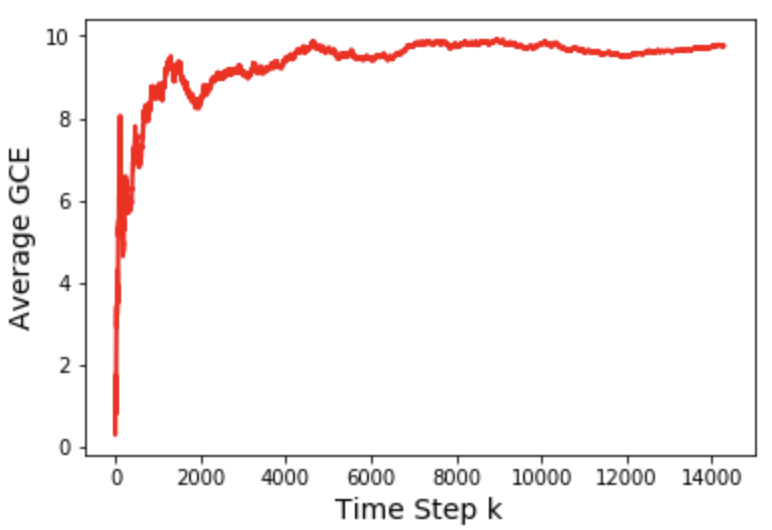
(a) Sample path of average GCE (24)

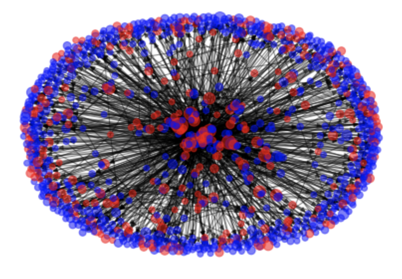
(b) Snapshot of nodes indicating page-rank

Just because blue nodes exhibit heterophily, GCE does not necessarily emerge. One can construct examples where blue nodes are heterophilic and yet GCE does not emerge. Thus GCE is subtle and non-trivial in directed networks such as Twitter and requires careful analysis.

Figure 10: Emergence of average glass ceiling effect in directed network using model in [138]. Fig.10(a) shows that red nodes achieve 10 times more influence than blue nodes despite being only 20% of the population. In Fig.10(b), the size of each node indicates its page-rank centrality. Minority red take on important centrality positions.

Summary

Part 3 discussed social sensing on large (random) graphs. The key ideas involve adaptively estimating degree distributions (via stochastic approximation algorithms), tracking infected degree distributions using mean field dynamics as a generative model, and a comparison of how the graph structure affects estimates. We also discussed how the glass ceiling effect emerges in social networks.

There are several other interesting sociological effects that can be modeled via dynamic models in social networks. [124] shows how using Markov random bridges (which are one dimensional Markov random fields), one can model echo chambers in social networks. [125] also shows how segregation in social networks can be mitigated by providing incentives to agents (the formulation involves an edge formation game).

5 Part 4. Polling Social Networks – The Friendship Paradox

Our final theme in this paper studies statistical estimation algorithms for polling nodes in a social network. We view polling as a generalization of information fusion (Theme 1) with the flexibility of who to poll and what question to ask. In large social networks, only a fraction of nodes can be polled to determine their decisions. Which nodes should be polled to achieve a statistically accurate estimate of phenomena such as the glass ceiling effect? A related question is: What question to ask the polled nodes? Nodes often have social desirability bias, i.e., they are embarrassed/reluctant to reveal their true voting intention; this can result in inaccurate poll estimates. How to provide incentives to nodes so that they reveal their true opinion?

Background. Consider a social network represented by a graph $G=(V,E)$ where each node $v\in V$ has a binary label $f(v)\in\{0,1\}$, representing for example the intention to vote for a certain political party, or infected with a disease. The aim of randomized polling of a social network (with possibly unknown structure) is to estimate the fraction of nodes with label 1 by polling only a subset of nodes, i.e.,

$$\bar{f}=\frac{|\{v\in V:f(v)=1\}|}{|V|},$$ (26)

Three widely used polling strategies are [157, 54]:

• Each uniformly sampled node is asked: Who will you vote for? The average $\hat{f}={\sum_{u\in S}f(u)}/{|S|}$, is used as the estimate of the fraction $\bar{f}$. The sample size to achieve error $\epsilon$ is $O(\frac{1}{\epsilon^{2}})$.

• Each uniformly sampled node is asked: Who do you think will win? Intuitively, EP is more accurate than IP since each node considers its own intent together with the intents of its friends. But this is not always true [54]; certain network structures can increase the bias of EP.

• To reduce the bias and variance of EP, [54] proposes an extension of EP called social sampling. The response of each sampled node is weighted by the labels and degrees of its neighbors.

These polling methods have limitations. First, EP and SS require the pollster to have significant information about the network structure to reduce bias and variance. Also, IP requires large number of sampled nodes to achieve a desired accuracy. Second, IP and SS do not take the privacy of the nodes into account. Attributes such as voting preferences are privacy sensitive and may lead to people falsely responding to the polls.

We aim to construct and analyze polling algorithms based on the friendship paradox and strategic querying to elicit truthful responses. In future work we will investigate controlled correlated polling strategies that optimize a multi-horizon objective. These correlated polling strategies are similar to respondent driven sampling [79, 80, 70] which is used by the US Center for Disease Control to sample from marginalized populations.

Friendship Paradox based Polling in Social Networks

The friendship paradox was discovered by Feld [64] and informally states “on average, your friends have more friends than you do”. A nicely packaged formulation in terms of stochastic dominance is [40]:

Theorem 5.1.

(Friendship Paradox [40]) Let ${G=(V,E)}$ be an undirected graph.

1. Let random variable $X$ denote a uniformly chosen node from $V$.

2. Let random variable $Y$ denote a uniformly chosen node from a uniformly chosen edge $e\in E$.

3. Let $Z$ denote a uniformly chosen neighbor (friend) of a uniformly chosen node from $V$.

Then, with $d(X)$ denoting the degree of node $X$ and $\geq_{s}$ denoting first order stochastic dominance [135]

$$d(Y)\geq_{s}d(X),\quad\text{ and }d(Z)\geq_{s}d(X)$$

Therefore, the expected degree of $Z$ and expected degree of $Y$ are larger than the expected degree of $X$.∎

[7] studies friendship paradox based polling in directed graphs. Specifically, in [7, 139, 140] we have developed the following Network Expectation Polling (NEP) algorithm:

1. Choose the node $Y$ or $Z$ in Theorem 5.1. Note that $Y$ and $Z$ are non-uniform samplers of nodes (unlike $X$). Also $Y$ and $Z$ can be sampled without knowing the network structure (see below).

2. Ask the sampled node: What fraction of your friends will vote for candidate $A$?

How to implement Step 1? Sampling $Y$ in Step 1 is equivalent to sampling from the stationary distribution of a random walk on the graph [56]; the convergence rate depends on the second largest eigenvalue of the graph Laplacian. So the implementation of Step 1 for $Y$ is simple: just walk through the network and compute the average of responses. Sampling $Z$ involves choosing a random friend of a randomly sampled node.

[7] proves that NEP outperforms intent and expectation polling in terms of mean squared error, recall Fig.11. Also the sampled node responds with the average of its friends’ opinions (rather than its own opinion); so nodes can truthfully reveal politically incorrect opinions without personal embarrassment.

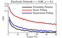
Figure 11: Friendship paradox based polling vs Intent and Expectation Polling (from [7]). $r$ and $\rho$ denote the assortative coefficient and degree label correlation. The Facebook dataset is from [117].

In [141] the friendship paradox poling is used in estimating the opinions of nodes when information diffuses in social network with monophilic contagion.

6 Closing Comments

This paper has surveyed four important aspects of social learning and social networks, namely, classical social learning, social learning with anticipatory agents, dynamics of social networks, and polling social networks.

One area we have not discussed is inference of optimal behavior of agents in a social network. This is driven both by technological advances such as the requirement for adaptively caching information in wireless networks [85], and also for modeling the user engagement in social multimedia networks [68, 83, 84]. These involve inverse reinforcement learning and revealed preference.

References

- [1] D. Acemoglu, M. Dahleh, I. Lobel, and A. Ozdaglar. Bayesian learning in social networks. The Review of Economic Studies, 78(4):1201–1236, 2011.
- [2] D. Acemoglu and A. Ozdaglar. Opinion dynamics and learning in social networks. Dynamic Games and Applications, 1(1):3–49, 2011.
- [3] D. Acemoglu, A. Ozdaglar, and A. Tahbaz-Salehi. Cascades in networks and aggregate volatility. Technical report, National Bureau of Economic Research, 2010.
- [4] A. Adams, L. Cherchye, B. De Rock, and E. Verriest. Consume now or later? time inconsistency, collective choice, and revealed preference. American Economic Review, 104(12):4147–83, 2014.
- [5] D. Aerts, J. Broekaert, M. Czachor, and B. D’Hooghe. A quantum-conceptual explanation of violations of expected utility in economics. In International Symposium on Quantum Interaction, pages 192–198. Springer, 2011.
- [6] R. Albert and A.-L. Barabási. Statistical mechanics of complex networks. Reviews of modern physics, 74(1):47, 2002.
- [7] N. Alipourfard, B. Nettasinghe, A. Abeliuk, V. Krishnamurthy, and K. Lerman. Friendship paradox biases perceptions in directed networks. Nature communications, 11(1):1–9, 2020.
- [8] N. Alipourfard, B. Nettasinghe, V. Krishnamurthy, and K. Lerman. Emergence of gender disparities in scientific citations. Nature communications, 2022. under revision.
- [9] R. Amir. Supermodularity and complementarity in economics: An elementary survey. Southern Economic Journal, 71(3):636–660, 2005.
- [10] M. S. Andersland and D. Teneketzis. Measurement scheduling for recursive team estimation. Journal of Optimization Theory and Applications, 89(3):615–636, June 1996.
- [11] P. Artzner, F. Delbaen, J. Eber, and D. Heath. Coherent measures of risk. Risk management: value at risk and beyond, page 145, 2002.
- [12] P. Artzner, F. Delbaen, J. Eber, D. Heath, and H. Ku. Coherent multiperiod risk adjusted values and bellman’s principle. Annals of Operations Research, 152(1):5–22, 2007.
- [13] S. Athey. Monotone comparative statics under uncertainty. The Quarterly Journal of Economics, 117(1):187–223, 2002.
- [14] R. J. Aumann. Agreeing to disagree. The Annals of Statistics, 4(6):1236–1239, Nov. 1976.
- [15] R. J. Aumann. Correlated equilibrium as an expression of Bayesian rationality. Econometrica, 55(1):1–18, 1987.
- [16] C. Avin, H. Daltrophe, B. Keller, Z. Lotker, C. Mathieu, D. Peleg, and Y.-A. Pignolet. Mixed preferential attachment model: Homophily and minorities in social networks. Physica A: Statistical Mechanics and its Applications, page 124723, 2020.
- [17] C. Avin, B. Keller, Z. Lotker, C. Mathieu, D. Peleg, and Y.-A. Pignolet. Homophily and the glass ceiling effect in social networks. In Proceedings of the 2015 conference on innovations in theoretical computer science, pages 41–50, 2015.
- [18] C. Avin, Z. Lotker, D. Peleg, Y.-A. Pignolet, and I. Turkel. Elites in social networks: An axiomatic approach to power balance and price’s square root law. PloS one, 13(10):e0205820, 2018.
- [19] A. Banerjee. A simple model of herd behavior. Quaterly Journal of Economics, 107(3):797–817, August 1992.
- [20] T. Banerjee and V. Veeravalli. Data-efficient quickest change detection with on-off observation control. Sequential Analysis, 31:40–77, 2012.
- [21] A. Barabási and R. Albert. Emergence of scaling in random networks. Science, 286(5439):509–512, 1999.
- [22] R. Bénabou and J. Tirole. Mindful economics: The production, consumption, and value of beliefs. Journal of Economic Perspectives, 30(3):141–64, 2016.
- [23] M. Benaim, J. Hofbauer, and S. Sorin. Stochastic approximations and differential inclusions. SIAM Journal on Control and Optimization, 44(1):328–348, 2005.
- [24] M. Benaim, J. Hofbauer, and S. Sorin. Stochastic approximations and differential inclusions, Part II: Applications. Mathematics of Operations Research, 31(3):673–695, 2006.
- [25] M. Benaim and J. Weibull. Deterministic approximation of stochastic evolution in games. Econometrica, 71(3):873–903, 2003.
- [26] A. Bensoussan. Stochastic Control of Partially Observable Systems. Cambridge University Press, Cambridge, UK, 1992.
- [27] A. Benveniste, M. Metivier, and P. Priouret. Adaptive Algorithms and Stochastic Approximations, volume 22 of Applications of Mathematics. Springer-Verlag, 1990.
- [28] S. Bhatt and V. Krishnamurthy. Adaptive polling in hierarchical social networks using blackwell dominance. IEEE Transactions on Signal and Information Processing over Networks, 5(3):538–553, 2019.
- [29] S. Bhatt and V. Krishnamurthy. Controlled sequential information fusion with social sensors. IEEE Transactions on Automatic Control, 66(12):5893–5908, 2020.
- [30] S. Bikchandani, D. Hirshleifer, and I. Welch. A theory of fads, fashion, custom, and cultural change as information cascades. Journal of Political Economy, 100(5):992–1026, October 1992.
- [31] T. Björk and A. Murgoci. A theory of Markovian time-inconsistent stochastic control in discrete time. Finance and Stochastics, 18(3):545–592, 2014.
- [32] D. Blackwell. Equivalent comparisons of experiments. The Annals of Mathematical Statistics, pages 265–272, 1953.
- [33] E. Blasch, E. Bossé, and D. Lambert. High-level information fusion management and systems design. Artech House, 2012.
- [34] A. Broder, R. K. amd F. Maghoul, P. Raghavan, S. Rajagopalan, R. Stata, A. Tomkins, and J. Wiener. Graph structure in the web. Computer networks, 33(1):309–320, 2000.
- [35] M. K. Brunnermeier, F. Papakonstantinou, and J. A. Parker. Optimal time-inconsistent beliefs: Misplanning, procrastination, and commitment. Management Science, 63(5):1318–1340, 2017.
- [36] M. K. Brunnermeier and J. A. Parker. Optimal expectations. The American Economic Review, 95(4):1092–1118, 2005.
- [37] S. Bubeck and N. Cesa-Bianchi. Regret analysis of stochastic and nonstochastic multi-armed bandit problems. arXiv preprint arXiv:1204.5721, 2012.
- [38] J. Busemeyer and P. Bruza. Quantum Models of Cognition and Decision. Quantum Models of Cognition and Decision. Cambridge University Press, 2012.
- [39] J. R. Busemeyer, E. M. Pothos, R. Franco, and J. S. Trueblood. A quantum theoretical explanation for probability judgment errors. Psychological review, 118(2):193, 2011.
- [40] Y. Cao and S. Ross. The friendship paradox. Mathematical Scientist, 41(1), 2016.
- [41] A. Caplin and M. Dean. Revealed preference, rational inattention, and costly information acquisition. The American Economic Review, 105(7):2183–2203, 2015.
- [42] A. Caplin, M. Dean, and J. Leahy. Rational inattention, optimal consideration sets, and stochastic choice. The Review of Economic Studies, 86(3):1061–1094, 2019.
- [43] A. Caplin and J. Leahy. Psychological expected utility theory and anticipatory feelings. The Quarterly Journal of Economics, 116(1):55–79, 2001.
- [44] M. Caplin and A. Dean. The behavioral implications of rational inattention with Shannon entropy. 2013.
- [45] A. R. Cassandra. Exact and Approximate Algorithms for Partially Observed Markov Decision Process. PhD thesis, Dept. Computer Science, Brown University, 1998.
- [46] O. Cavus and A.Ruszczynski. Risk-averse control of undiscounted transient Markov models. SIAM Journal on Control and Optimization, 52(6):3935–3966, 2014.
- [47] B. Çelen and S. Kariv. Distinguishing informational cascades from herd behavior in the laboratory. The American Economic Review, 94(3):484–498, 2004.
- [48] C. Chamley. Rational herds: Economic Models of Social Learning. Cambridge University Press, 2004.
- [49] C. J. Charpentier, E. S. Bromberg-Martin, and T. Sharot. Valuation of knowledge and ignorance in mesolimbic reward circuitry. Proceedings of the National Academy of Sciences, 115(31):E7255–E7264, 2018.
- [50] Z. Cheng, J. Caverlee, and K. Lee. You are where you tweet: A content-based approach to geo-locating Twitter users. In Proceedings of the 19th ACM International Conference on Information and Knowledge Management, pages 759–768. ACM, 2010.
- [51] F. Chung and L. Lu. Complex Graphs and Networks. Conference Board of the Mathematical Sciences, National Science Foundation (U.S.), 2006.
- [52] R. A. Cohn, W. G. Lewellen, R. C. Lease, and G. G. Schlarbaum. Individual investor risk aversion and investment portfolio composition. The Journal of Finance, 30(2):605–620, 1975.
- [53] J. O. Cook and L. W. Barnes Jr. Choice of delay of inevitable shock. Journal of Abnormal and Social Psychology, 68(6):669–672, 1964.
- [54] A. Dasgupta, R. Kumar, and D. Sivakumar. Social sampling. In Proceedings of the 18th ACM SIGKDD international conference on Knowledge discovery and data mining, pages 235–243, Beijing, 2012. ACM.
- [55] B. . Donkers and A. Soest. Subjective measures of household preferences and financial decisions. Journal of Economic Psychology, 20(6):613 – 642, 1999.
- [56] R. Durrett. Probability: theory and examples, volume 49. Cambridge university press, 2019.
- [57] D. Easley and J. Kleinberg. Networks, Crowds, and Markets: Reasoning About a Highly Connected World. Cambridge University Press, 2010.
- [58] R. J. Elliott, L. Aggoun, and J. B. Moore. Hidden Markov Models – Estimation and Control. Springer-Verlag, New York, 1995.
- [59] G. Ellison and D. Fudenberg. Rules of thumb for social learning. Journal of Political Economy, 101(4):pp. 612–643, 1993.
- [60] Y. Ephraim and N. Merhav. Hidden Markov processes. IEEE Transactions on Information Theory, 48:1518–1569, June 2002.
- [61] P. Erdős and A. Rényi. On the evolution of random graphs. Publ. Math. Inst. Hungar. Acad. Sci, 5:17–61, 1960.
- [62] E. Ert, A. Fleischer, and N. Magen. Trust and reputation in the sharing economy: The role of personal photos in airbnb. Tourism Management, 55:62–73, 2016.
- [63] S. N. Ethier and T. G. Kurtz. Markov Processes—Characterization and Convergence. Wiley, 1986.
- [64] S. L. Feld. Why your friends have more friends than you do. American Journal of Sociology, 96(6):1464–1477, 1991.
- [65] E. Fernandez-Gaucherand and S. Marcus. Risk-sensitive optimal control of hidden Markov models: Structural results. IEEE Transactions on Automatic Control, 42(10):1418–1422, 1997.
- [66] D. Fudenberg and D. K. Levine. The Theory of Learning in Games. MIT Press, 1998.
- [67] J.-J. Ganuza and J. S. Penalva. Signal orderings based on dispersion and the supply of private information in auctions. Econometrica, 78(3):1007–1030, 2010.
- [68] O. Gharehshiran, W. Hoiles, and V. Krishnamurthy. Detection of homophilic communities and coordination of interacting meta-agents: A game-theoretic viewpoint. IEEE Transactions on Signal and Information Processing over Networks, 2(1):84–101, 2016.
- [69] O. N. Gharehshiran, V. Krishnamurthy, and G. Yin. Adaptive search algorithms for discrete stochastic optimization: A smooth best-response approach. IEEE Transactions on Automatic Control, 62(1):161–176, 2017.
- [70] S. Goel and M. J. Salganik. Respondent-driven sampling as Markov chain Monte Carlo. Statistics in Medicine, 28:2209–2229, 2009.
- [71] B. Golub and M. Jackson. How homophily affects the speed of learning and best response dynamics. 2012.
- [72] L. Guo, L. Ljung, and G. J. Wang. Necessary and sufficient conditions for stability of lms. IEEE Transactions on Automatic Control,, 42(6):761–770, 1997.
- [73] M. Hamdi, V. Krishnamurthy, and G. Yin. Tracking a Markov-modulated stationary degree distribution of a dynamic random graph. IEEE Transactions on Information Theory, 60(10):6609–6625, 2014.
- [74] M. Hamdi, G. Solman, A. Kingstone, and V. Krishnamurthy. Social learning in a human society: An experimental study. arXiv preprint arXiv:1408.5378, 2014.
- [75] L. Hansen and T. Sargent. Robust control and model uncertainty. The American Economic Review, 91(2):60–66, 2001.
- [76] S. Hart and A. Mas-Colell. A simple adaptive procedure leading to correlated equilibrium. Econometrica, 68(5):1127–1150, 2000.
- [77] S. Hart and A. Mas-Colell. A general class of adaptive strategies. Journal of Economic Theory, pages 26–54, 2001.
- [78] S. Hart, A. Mas-Colell, and Y. Babichenko. Simple Adaptive Strategies: From Regret-Matching to Uncoupled Dynamics, volume 4 of World Scientific Series in Economic Theory. World Scientific Publishing, 2013.
- [79] D. D. Heckathorn. Respondent-driven sampling: a new approach to the study of hidden populations. Social Problems, 44:174–199, 1997.
- [80] D. D. Heckathorn. Respondent-driven sampling II: deriving valid population estimates from chain-referral samples of hidden populations. Social Problems, 49:11–34, 2002.
- [81] M. Hernández-González and M. Basin. Discrete-time filtering for nonlinear polynomial systems over linear observations. International Journal of Systems Science, 45(7):1461–1472, 2014.
- [82] J. Hofbauer and W. Sandholm. On the global convergence of stochastic fictitious play. Econometrica, 70(6):2265–2294, Nov. 2002.
- [83] W. Hoiles, A. Aprem, and V. Krishnamurthy. Engagement and popularity dynamics of youtube videos and sensitivity to meta-data. IEEE Transactions on Knowledge & Data Engineering, (7):1426–1437, 2017.
- [84] W. Hoiles, V. Krishnamurthy, and K. Pattanayak. Rationally inattentive inverse reinforcement learning explains YouTube commenting behavior. Journal of Machine Learning Research, 21(170):1–39, 2020.
- [85] W. Hoiles, O. Namvar, V. Krishnamurthy, N. Dao, and H. Zhang. Adaptive caching in the youtube content distribution network: A revealed preference game-theoretic learning approach. IEEE Transactions on Cognitive Communications and Networking, 1(1):71–85, 2015.
- [86] H. Ibarra. Paving an alternative route: Gender differences in managerial networks. Social psychology quarterly, pages 91–102, 1997.
- [87] M. Jackson. Social and Economic Networks. Princeton University Press, 2010.
- [88] A. Jadbabaie, P. Molavi, and A. Tahbaz-Salehi. Information heterogeneity and the speed of learning in social networks. Columbia Business School Research Paper, (13-28), 2013.
- [89] M. James, J. Baras, and R. Elliott. Risk-sensitive control and dynamic games for partially observed discrete-time nonlinear systems. IEEE Transactions on Automatic Control, 39(4):780–792, April 1994.
- [90] D. Kahneman and A. Tversky. Prospect theory: An analysis of decision under risk. Econometrica, 47(2):263–291, 1979.
- [91] Y. Kanoria and O. Tamuz. Tractable Bayesian social learning on trees. In Proceedings of the IEEE International Symposium on Information Theory (ISIT), pages 2721 –2725, Jul. 2012.
- [92] Y. Kanoria and O. Tamuz. Tractable Bayesian social learning on trees. IEEE Journal on Selected Areas Communications, 31(4):756–765, 2013.
- [93] D. Kempe, J. Kleinberg, and E. Tardos. Maximizing the spread of influence through a social network. In Proceedings of the 9th ACM SIGKDD International Conference on Knowledge Discovery and Data Mining, pages 137–146, Washington, DC, Aug 2003.
- [94] A. Khrennikov. Ubiquitous quantum structure. Springer, 2010.
- [95] A. Y. Khrennikov and E. Haven. Quantum mechanics and violations of the sure-thing principle: The use of probability interference and other concepts. Journal of Mathematical Psychology, 53(5):378–388, 2009.
- [96] B. King-Casas, D. Tomlin, C. Anen, C. CamererF, S. Quartz, , and P. Montague. Getting to know you: reputation and trust in a two-person economic exchange. Science, 308(5718):78–83, 2005.
- [97] V. Krishnamurthy. Bayesian sequential detection with phase-distributed change time and nonlinear penalty – a lattice programming POMDP approach. IEEE Transactions on Information Theory, 57(3):7096–7124, Oct. 2011.
- [98] V. Krishnamurthy. Quickest detection POMDPs with social learning: Interaction of local and global decision makers. IEEE Transactions on Information Theory, 58(8):5563–5587, 2012.
- [99] V. Krishnamurthy. How to schedule measurements of a noisy Markov chain in decision making? IEEE Transactions on Information Theory, 59(9):4440–4461, July 2013.
- [100] V. Krishnamurthy. Partially Observed Markov Decision Processes. From Filtering to Controlled Sensing. Cambridge University Press, 2016.
- [101] V. Krishnamurthy. Convex stochastic dominance in bayesian localization, filtering and controlled sensing POMDPs. IEEE Transactions on Information Theory, 66(5):3187–3201, 2019.
- [102] V. Krishnamurthy. Quickest change detection of time inconsistent anticipatory agents. human-sensor and cyber-physical systems. IEEE Transactions on Signal Processing, 59:1054–1069, 2021.
- [103] V. Krishnamurthy and F. V. Abad. Gradient based policy optimization of constrained unichain Markov decision processes. In S. Cohen, D. Madan, and T. Siu, editors, Stochastic Processes, Finance and Control: A Festschrift in Honor of Robert J. Elliott. World Scientific, 2012. http://arxiv.org/abs/1110.4946.
- [104] V. Krishnamurthy, A. Aprem, and S. Bhatt. Multiple stopping time pomdps: Structural results & application in interactive advertising on social media. Automatica, 95:385–398, 2018.
- [105] V. Krishnamurthy and S. Bhatt. Sequential detection of market shocks with risk-averse cvar social sensors. IEEE Journal of Selected Topics in Signal Processing, 10(6):1061–1072, 2016.
- [106] V. Krishnamurthy, S. Bhatt, and T. Pedersen. Tracking infection diffusion in social networks: Filtering algorithms and threshold bounds. IEEE Transactions on Signal and Information Processing over Networks, 3(2):298–315, 2017.
- [107] V. Krishnamurthy and D. Djonin. Structured threshold policies for dynamic sensor scheduling–a partially observed Markov decision process approach. IEEE Transactions on Signal Processing, 55(10):4938–4957, Oct. 2007.
- [108] V. Krishnamurthy and D. Djonin. Optimal threshold policies for multivariate POMDPs in radar resource management. IEEE Transactions on Signal Processing, 57(10), 2009.
- [109] V. Krishnamurthy, O. N. Gharehshiran, and M. Hamdi. Interactive sensing and decision making in social networks. Foundations and Trends® in Signal Processing, 7(1-2):1–196, 2014.
- [110] V. Krishnamurthy and W. Hoiles. Online reputation and polling systems: Data incest, social learning and revealed preferences. IEEE Transactions Computational Social Systems, 1(3):164–179, Jan. 2015.
- [111] V. Krishnamurthy and U. Pareek. Myopic bounds for optimal policy of POMDPs: An extension of Lovejoy’s structural results. Operations Research, 62(2):428–434, 2015.
- [112] V. Krishnamurthy and H. V. Poor. Social learning and Bayesian games in multiagent signal processing: How do local and global decision makers interact? IEEE Signal Processing Magazine, 30(3):43–57, 2013.
- [113] V. Krishnamurthy, K. Topley, and G. Yin. Consensus formation in a two-time-scale Markovian system. SIAM Journal Multiscale Modeling and Simulation, 7(4):1898–1927, 2009.
- [114] H. J. Kushner and A. Shwartz. Stochastic approximation in Hilbert space: Identification and optimization of linear continuous parameter systems. SIAM journal on control and optimization, 23(5):774–793, 1985.
- [115] H. J. Kushner and G. Yin. Stochastic Approximation Algorithms and Recursive Algorithms and Applications. Springer-Verlag, 2nd edition, 2003.
- [116] E. L. Lehmann. Comparing location experiments. Annals of Statistics, 16(2):521–533, 1988.
- [117] J. Leskovec and J. J. Mcauley. Learning to discover social circles in ego networks. In Advances in neural information processing systems, pages 539–547, 2012.
- [118] D. López-Pintado. Contagion and coordination in random networks. International Journal of Game Theory, 34(3):371–381, 2006.
- [119] D. López-Pintado. Diffusion in complex social networks. Games and Economic Behavior, 62(2):573–590, 2008.
- [120] D. López-Pintado. An overview of diffusion in complex networks. In Complex Networks and Dynamics, pages 27–48. Springer, 2016.
- [121] W. S. Lovejoy. On the convexity of policy regions in partially observed systems. Operations Research, 35(4):619–621, July-August 1987.
- [122] W. S. Lovejoy. Some monotonicity results for partially observed Markov decision processes. Operations Research, 35(5):736–743, Sept.-Oct. 1987.
- [123] W. S. Lovejoy. A survey of algorithmic methods for partially observed Markov decision processes. Annals of Operations Research, 28:47–66, 1991.
- [124] R. Luo, B. Nettasinghe, and V. Krishnamurthy. Echo chambers and segregation in social networks: Markov bridge models and estimation. IEEE Transactions Computational Social Systems, 2021.
- [125] R. Luo, B. Nettasinghe, and V. Krishnamurthy. Controlling segregation in social network dynamics as an edge formation game. IEEE Transactions on Network Science and Engineering, 2022.
- [126] M. McPherson, L. Smith-Lovin, and J. M. Cook. Birds of a feather: Homophily in social networks. Annual review of sociology, 27(1):415–444, 2001.
- [127] P. Milgrom. Good news and bad news: Representation theorems and applications. Bell Journal of Economics, 12(2):380–391, 1981.
- [128] S. M. Miller and C. E. Mangan. Interacting effects of information and coping style in adapting to gynecologic stress: should the doctor tell all? Journal of personality and social psychology, 45(1):223–236, 1983.
- [129] S. Mitra and T. Ji. Risk measures in quantitative finance. International Journal of Business Continuity and Risk Management, 1(2):125–135, 2010.
- [130] I. Mohr. Going viral: An analysis of youtube videos. Journal of Marketing Development and Competitiveness, 8(3):43, 2014.
- [131] P. Molavi, A. Tahbaz-Salehi, and A. Jadbabaie. A theory of non-bayesian social learning. Econometrica, 86(2):445–490, 2018.
- [132] G. V. Moustakides. Exponential convergence of products of random matrices: Application to adaptive algorithms. International Journal of Adaptive Control and Signal Processing, 12(7):579–597, 1998.
- [133] M. Mueller-Frank. A general framework for rational learning in social networks. Theoretical Economics, 8(1):1–40, 2013.
- [134] L. Mui, M. Mohtashemi, and A. Halberstadt. A computational model of trust and reputation. In Proceedings of the 35th Annual Hawaii International Conference on System Sciences, pages 2431–2439. IEEE, 2002.
- [135] A. Muller and D. Stoyan. Comparison Methods for Stochastic Models and Risk. Wiley, 2002.
- [136] O. Namvar, V. Krishnamurthy, and G. Yin. Distributed energy-aware diffusion least mean squares: Game-theoretic learning. IEEE Journal of Selected Topics in Signal Processing, 7(5):821, 2013.
- [137] O. Namvar, V. Krishnamurthy, and G. Yin. Distributed tracking of correlated equilibria in regime switching noncooperative games. IEEE Transactions on Automatic Control, 58(10):2435–2450, 2013.
- [138] B. Nettasinghe, N. Alipourfard, S. Iota, V. Krishnamurthy, and K. Lerman. Scale-free degree distributions, homophily and the glass ceiling effect in directed networks. Journal of Complex Networks, 10(2):cnac007, 2022.
- [139] B. Nettasinghe and V. Krishnamurthy. What do your friends think?: Efficient polling methods for networks using friendship paradox. IEEE Transactions on Knowledge and Data Engineering, 2019.
- [140] B. Nettasinghe and V. Krishnamurthy. Maximum likelihood estimation of power-law degree distributions via friendship paradox-based sampling. ACM Transactions Knowledge Discovery from Data, 15(6):1–28, 2021.
- [141] B. Nettasinghe, V. Krishnamurthy, and K. Lerman. Diffusion in social networks: Effects of monophilic contagion, friendship paradox and reactive networks. IEEE Transactions on Network Science and Engineering, 7(3):1121–1132, 2019.
- [142] S. Nilizadeh, A. Groggel, P. Lista, S. Das, Y.-Y. Ahn, A. Kapadia, and F. Rojas. Twitter’s glass ceiling: The effect of perceived gender on online visibility. 2016.
- [143] C. Nowzari, V. Preciado, and G. Pappas. Optimal resource allocation for control of networked epidemic models. 2015.
- [144] C. H. Papadimitriou and J. Tsitsiklis. The compexity of Markov decision processes. Mathematics of Operations Research, 12(3):441–450, 1987.
- [145] A. Park and H. Sabourian. Herding and contrarian behavior in financial markets. Econometrica, 79(4):973–1026, 2011.
- [146] R. Pastor-Satorras and A. Vespignani. Epidemic spreading in scale-free networks. Physical Review Letters, 86(14):3200, 2001.
- [147] I. Petersen, M. James, and P. Dupuis. Minimax optimal control of stochastic uncertain systems with relative entropy constraints. IEEE Transactions on Automatic Control, 45(3):398–412, 2000.
- [148] H. V. Poor. Quickest detection with exponential penalty for delay. Annals of Stastistics, 26(6):2179–2205, 1998.
- [149] H. V. Poor and O. Hadjiliadis. Quickest Detection. Cambridge University Press, 2008.
- [150] K. Premkumar, A. Kumar, and V. Veeravalli. Bayesian quickest transient change detection. In International Workshop on Applied Probability, Madrid, July 2010.
- [151] M. Raginsky. Shannon meets Blackwell and Le Cam: Channels, codes, and statistical experiments. In Proceedings of 2011 IEEE International Symposium on Information Theory Proceedings (ISIT), pages 1220–1224. IEEE, 2011.
- [152] U. Rieder. Structural results for partially observed control models. Methods and Models of Operations Research, 35(6):473–490, 1991.
- [153] U. Rieder and R. Zagst. Monotonicity and bounds for convex stochastic control models. Mathematical Methods of Operations Research, 39(2):187–207, June 1994.
- [154] R. T. Rockafellar and S. Uryasev. Optimization of conditional value-at-risk. Journal of risk, 2:21–42, 2000.
- [155] R. T. Rockafellar and S. Uryasev. Conditional value-at-risk for general loss distributions. Journal of banking & finance, 26(7):1443–1471, 2002.
- [156] D. Rosenberg, E. Solan, and N. Vieille. Informational externalities and emergence of consensus. Games and Economic Behavior, 66(2):979–994, 2009.
- [157] D. Rothschild and J. Wolfers. Forecasting elections: Voter intentions versus expectations, 2010.
- [158] A. Ruszczyński. Risk-averse dynamic programming for Markov decision processes. Mathematical programming, 125(2):235–261, 2010.
- [159] T. Sakaki, M. Okazaki, and Y. Matsuo. Earthquake shakes Twitter users: real-time event detection by social sensors. In Proceedings of the 19th International Conference on World Wide Web, pages 851–860, New York, NY, USA, 2010. ACM.
- [160] D. Savage, X. Zhang, X. Yu, P. Chou, and Q. Wang. Anomaly detection in online social networks. Social Networks, 39:62–70, 2014.
- [161] A. H. Sayed. Adaptation, learning, and optimization over networks. Foundations and Trends in Machine Learning, 7(4–5):311–801, 2014.
- [162] E. Shafieepoorfard, M. Raginsky, and S. P. Meyn. Rationally inattentive control of markov processes. SIAM Journal on Control and Optimization, 54(2):987–1016, 2016.
- [163] A. N. Shiryaev. On optimum methods in quickest detection problems. Theory of Probability and its Applications, 8(1):22–46, 1963.
- [164] D. J. Simons and R. A. Rensink. Change blindness: Past, present, and future. Trends in cognitive sciences, 9(1):16–20, 2005.
- [165] C. Sims. Implications of rational inattention. Journal of Monetary Economics, 50(3):665–690, 2003.
- [166] C. A. Sims. Rational inattention and monetary economics. In Handbook of monetary Economics, volume 3, pages 155–181. Elsevier, 2010.
- [167] J. E. Smith and K. F. McCardle. Structural properties of stochastic dynamic programs. Operations Research, 50(5):796–809, 2002.
- [168] L. Smith and P. Sorenson. Pathological outcomes of observational learning. Econometrica, 68(2):371–398, 2000.
- [169] L. Snow, V. Krishnamurthy, and B. M. Sadler. Quickest detection for human-sensor systems using quantum decision theory. arXiv preprint 2208.08583, 2022.
- [170] J. Spall. Introduction to Stochastic Search and Optimization. Wiley, 2003.
- [171] P. E. Stephan and S. G. Levin. Leaving careers in it: Gender differences in retention. The Journal of Technology Transfer, 30(4):383–396, 2005.
- [172] A.-A. Stoica, C. Riederer, and A. Chaintreau. Algorithmic glass ceiling in social networks: The effects of social recommendations on network diversity. In Proceedings of the 2018 World Wide Web Conference, pages 923–932, 2018.
- [173] A. Tartakovsky and G. Moustakides. State-of-the-art in bayesian changepoint detection. Sequential Analysis, 29(2):125–145, 2010.
- [174] D. Teneketzis and P. Varaiya. The decentralized quickest detection problem. IEEE Transactions on Automatic Control, 29(7):641–644, 1984.
- [175] P. Tichavsky, C. H. Muravchik, and A. Nehorai. Posterior Cramér-Rao bounds for discrete-time nonlinear filtering. IEEE Transactions on Signal Processing, 46(5):1386–1396, May 1998.
- [176] S. Tom, C. Fox, C. Trepel, and A. Poldrack. The neural basis of loss aversion in decision-making under risk. Science, 315(5811):515–518, 2007.
- [177] D. M. Topkis. Supermodularity and Complementarity. Princeton University Press, 1998.
- [178] J. S. Trueblood and J. R. Busemeyer. A quantum probability account of order effects in inference. Cognitive science, 35(8):1518–1552, 2011.
- [179] J. Tsitsiklis. Decentralized detection. Advances in Statistical Signal Processing, 2:297–344, 1993.
- [180] J. Unnikrishnan, V. Veeravalli, and S. Meyn. Minimax robust quickest change detection. IEEE Transactions on Information Theory, 57(3):1604–1614, 2011.
- [181] A. W. V. D. Vaart and J. Wellner. Weak convergence. In Weak Convergence and Empirical Processes, pages 16–28. Springer, 1996.
- [182] V. Veeravalli. Decentralized quickest change detection. IEEE Transactions on Information Theory, 47(4):1657–1665, 2001.
- [183] V. Veeravalli and T. Banerjee. Quickest change detection. Academic press library in signal processing: Array and statistical signal processing, 3:209–256, 2013.
- [184] F. Vega-Redondo. Complex Social Networks, volume 44. Cambridge University Press, 2007.
- [185] R. Viswanathan and P. Varshney. Distributed detection with multiple sensors I. Fundamentals. Proceedings of the IEEE, 85(1):54–63, 1997.
- [186] P. Wang and P. Djurić. Distributed Bayesian estimation of linear models with unknown observation covariances. IEEE Transactions on Signal Processing, 64(8):1962–1971, 2016.
- [187] J. D. West, J. Jacquet, M. M. King, S. J. Correll, and C. T. Bergstrom. The role of gender in scholarly authorship. PloS one, 8(7):e66212, 2013.
- [188] P. Whittle. Risk-sensitive linear/quadratic/gaussian control. Advances in Applied Probability, pages 764–777, 1981.
- [189] G. Yin, C. Ion, and V. Krishnamurthy. How does a stochastic optimization/approximation algorithm adapt to a randomly evolving optimum/root with jump Markov sample paths. Mathematical programming B. (Special Issue dedicated to B.T. Polyak’s 70th Birthday), 120(1):67–99, 2009.
- [190] G. Yin, V. Krishnamurthy, and C. Ion. Regime switching stochastic approximation algorithms with application to adaptive discrete stochastic optimization. SIAM Journal on Optimization, 14(4):117–1215, 2004.
- [191] V. I. Yukalov and D. Sornette. Mathematical structure of quantum decision theory. Advances in Complex Systems, 13(05):659–698, 2010.
- [192] V. I. Yukalov and D. Sornette. Quantitative predictions in quantum decision theory. IEEE Transactions on systems, man, and cybernetics: systems, 48(3):366–381, 2016.
- [193] Z. Zhang, E. K. P. Chong, A. Pezeshki, W. Moran, and S. Howard. Learning in hierarchical social networks. IEEE Journal on Selected Topics Signal Processing, 7(2):305–317, April 2013.