Hercules Against Data Series Similarity Search

Abstract.

We propose Hercules, a parallel tree-based technique for exact similarity search on massive disk-based data series collections. We present novel index construction and query answering algorithms that leverage different summarization techniques, carefully schedule costly operations, optimize memory and disk accesses, and exploit the multi-threading and SIMD capabilities of modern hardware to perform CPU-intensive calculations. We demonstrate the superiority and robustness of Hercules with an extensive experimental evaluation against state-of-the-art techniques, using many synthetic and real datasets, and query workloads of varying difficulty. The results show that Hercules performs up to one order of magnitude faster than the best competitor (which is not always the same). Moreover, Hercules is the only index that outperforms the optimized scan on all scenarios, including the hard query workloads on disk-based datasets. This paper was published in the Proceedings of the VLDB Endowment, Volume 15, Number 10, June 2022.

PVLDB Reference Format:
PVLDB, 15(10): 2005 - 2018, 2022.
doi:10.14778/3547305.3547308

PVLDB Artifact Availability:
The source code, data, and/or other artifacts have been made available at %leave␣empty␣if␣no␣availability␣url␣should␣be␣sethttp://www.mi.parisdescartes.fr/~themisp/hercules.

1. Introduction

Data series are one of the most common data types, covering virtually every scientific and social domain (Kashino et al., 1999; Shasha, 1999; Paraskevopoulos et al., 2013; Soldi et al., 2014; Mirylenka et al., 2016; Raza et al., 2015; Bach-Andersen et al., 2017; Knieling et al., 2017; Linardi et al., 2018; Laviron et al., 2021; Linardi et al., 2020; Boniol et al., 2022; Paparrizos et al., 2022). A data series is a sequence of ordered real values. When the sequence is ordered on time, it is called a time series. However, the order can be defined by other measures, such as angle or mass (Palpanas, 2016).

Motivation. Similarity search lies at the core of many critical data science applications related to data series (Palpanas, 2015; Zoumpatianos and Palpanas, 2018; Palpanas and Beckmann, 2019; Bagnall et al., 2019), but also in other domains, where data are represented as (or transformed to) high-dimensional vectors (Echihabi et al., 2020b, 2021b, 2021c). The problem of efficient similarity search over large series collections has been studied heavily in the past 30 years (Faloutsos et al., 1994; Shieh and Keogh, 2009; Wang et al., 2013; Linardi and Palpanas, 2018; Kondylakis et al., 2019; Palpanas, 2020; Echihabi, 2020; Gogolou et al., 2020; Yagoubi et al., 2017; Peng et al., 2021b; Levchenko et al., 2021; Chatzigeorgakidis et al., 2021; Peng et al., 2021a; Wang and Palpanas, 2021; Chatzigeorgakidis et al., 2022), and will continue to attract attention as massive sequence collections are becoming omnipresent in various domains (Palpanas and Beckmann, 2019; Bagnall et al., 2019).

Challenges. Designing highly-efficient disk-based data series indexes is thus crucial. ParIS+ (Peng et al., 2021c) is a disk-based data series parallel index, which exploited the parallelism capabilities provided by multi-socket and multi-core architectures. ParIS+ builds an index based on the iSAX summaries of the data series in the collection, whose leaves are populated only at search time. This results in a highly reduced cost for constructing the index, but as we will demonstrate, it often incurs a high query answering cost, despite the superior pruning ratio offered by the iSAX summaries (Echihabi et al., 2018).

For this reason, other data series indexes, such as DSTree (Wang et al., 2013), have recently attracted attention. Extensive experimental evaluations (Echihabi et al., 2018, 2019) have shown that sometimes DSTree exhibits better performance in query answering than iSAX-based indexes (like ParIS+). This is because DSTree spends a significant amount of time during indexing to adapt its splitting policy and node summarizations to the data distribution, leading to better data clustering (in the index leaf nodes), and thus more efficient exact query answering for workloads (Echihabi et al., 2018). In contrast, ParIS+ uses pre-defined split points and a fixed maximum resolution for the iSAX summaries. This helps ParIS+ build the index faster, but hurts the quality of data clustering. Therefore, similar data series may end up in different leaves, making query answering slower, especially on hard workloads that are the most challenging. As a result, no single data series similarity search indexing approach among the existing techniques wins across all popular query workloads (Echihabi et al., 2018).

The Hercules Approach. In this paper, we present Hercules, the first data series index that answers queries faster than all recent state-of-the-art techniques across all popular workloads. Hercules achieves this by exploiting the following key ideas. First, it leverages two different data series summarization techniques, EAPCA and iSAX, utilized by DSTree and ParIS+, respectively, to get a well-clustered tree structure during index building, and at the same time a high leaf pruning ratio during query answering. Hercules enjoys the advantages of both approaches and employs new ideas to overcome their limitations. Second, it exploits a two-level buffer management technique to optimize memory accesses. This design utilizes (i) a large memory buffer (HBuffer) which contains the raw data of all leaves and is flushed to disk whenever it becomes full, and (ii) a small buffer ( SBuffer) for each leaf containing pointers to the raw data of the leaf that are stored in HBuffer. This way, it reduces the number of system calls, guards against the occurrence of out-of-memory management issues, and improves the performance of index construction. It also performs scheduling of external storage requests more efficiently. While state-of-the-art techniques (Wang et al., 2013; Peng et al., 2021c) typically store the data of each leaf in a separate file, Hercules stores the raw data series in a single file, following the order of an inorder traversal of the tree leaves. This helps Hercules reduce the cost of random I/O operations, and efficiently support both easy and hard queries. Moreover, Hercules schedules costly operations (e.g., statistics updates, calculating iSAX summaries, etc.) more efficiently than in previous works (Wang et al., 2013; Peng et al., 2021c).

Last but not least, Hercules uses parallelization to accelerate the execution of CPU-intensive calculations. It does so judiciously, adapting its access path selection decisions to each query in a workload during query answering (e.g., Hercules decides on when to parallelize a query based on the pruning ratio of the data series summaries, EAPCA and iSAX), and carefully scheduling index insertions and disk flushes while guaranteeing data integrity. This required novel designs for the following reasons. The parallelization ideas utilized for state-of-the-art data series indexes (Peng et al., 2018, 2020, 2021c) are relevant to tree-based indexes with a very large root fanout (such as the iSAX-based indexes (Palpanas, 2020)). In such indexes, parallelization can be easily achieved by having different threads work in different root subtrees of the index tree. The Hercules index tree is an unbalanced binary tree, and thus it has a small fanout and uneven subtrees. In such index trees, heavier synchronization is necessary, as different threads may traverse similar paths and may need to process the same nodes. Moreover, working on trees of small fan-out may result in more severe load balancing problems.

Our experimental evaluation with synthetic and real datasets from diverse domains shows that , in terms of query efficiency, Hercules consistently outperforms both Paris+ (by 5.5x-63x) and our optimized implementation of DSTree (by 1.5x-10x). This is true for all synthetic and real query workloads of different hardness that we tried (note that all algorithms return the same, exact results).

Contributions. Our contributions are as follows:

$\bullet$ We propose a new parallel data series index that exhibits better query answering performance than all recent state-of-the-art approaches across all popular query workloads. The new index achieves better pruning than previous approaches by exploiting the benefits of two different summarization techniques, and a new query answering mechanism.

$\bullet$ We propose a new parallel data series index construction algorithm, which leverages a novel protocol for constructing the tree and flushing data to disk. This protocol achieves load balancing (among workers) on the binary index tree, due to a careful scheduling mechanism of costly operations.

$\bullet$ We realize an ablation study that explains the contribution of individual design choices to the final performance improvements for queries of different hardness, and could support further future advancements in the field.

$\bullet$ We demonstrate the superiority and robustness of Hercules with an extensive experimental evaluation against the state-of-the-art techniques, using a variety of synthetic and real datasets. The experiments, with query workloads of varying degrees of difficulty, show that Hercules is between 1.3x-9.4x faster than the best competitor, which is different for the different datasets and workloads. Hercules is also the only index that outperforms the optimized parallel scan on all scenarios, including the case of hard query workloads.

2. Preliminaries & Related Work

A data series $S(p_{1},p_{2},...,p_{n})$ is an ordered sequence of points, $p_{i}$, $1\leq i\leq n$. The number of points, $|S|=n$, is the length of the series. We use $\mathbb{S}$ to represent all the series in a collection (dataset). A data series of length $n$ is typically represented as a single point in an $n$-dimensional space. Then the values and length of $S$ are referred to as dimensions and dimensionality, respectively.

Data series similarity search is typically reduced to a k-Nearest Neighbor (k-NN) query. Given an integer $k$, a dataset $\mathbb{S}$ and a query series $S_{Q}$, a k-NN query retrieves the set of $k$ series $\mathbb{A}=\{\{S_{1},...,S_{k}\}\in\mathbb{S}~{}|~{}\forall\ S\in\mathbb{A}\ and\ \forall\ S^{\prime}\notin\mathbb{A},\ d(S_{Q},S)\leq d(S_{Q},S^{\prime})\}$, where $d(S_{Q},S_{C})$ is the distance between $S_{Q}$ and any data series $S_{C}\in\mathbb{S}$.

This work focuses on whole matching queries (i.e., compute similarity between an entire query series and an entire candidate series) using the Euclidean distance. Hercules can support any distance measure equipped with a lower-bounding distance, e.g. Dynamic Time Warping (DTW) (Keogh and Ratanamahatana, 2005) (similarly to how other indices support DTW (Peng et al., 2021a)).

Summarization Techniques. The Symbolic Aggregate Approximation (SAX) (Lin et al., 2003) first transforms a data series using Piecewise Aggregate Approximation (PAA) (Keogh et al., 2001). It divides the series into equi-length segments and represents each segment with one floating-point value corresponding to the mean of all the points belonging to the segment (Fig. 1(a)). The iSAX summarization reduces the footprint of the PAA representation by applying a discretization technique that maps PAA values to a discrete set of symbols (alphabet) that can be succinctly represented in binary form (Fig. 1(b)). Following previous work, we use 16 segments (Echihabi et al., 2018) and an alphabet size of 256 (Shieh and Keogh, 2008).

The Adaptive Piecewise Constant Approximation (APCA) (Chakrabarti et al., 2002) is a technique that approximates a series using variable-length segments. The approximation represents each segment with the mean value of its points (Fig. 1(c)). The Extended APCA (EAPCA) (Wang et al., 2013) represents each segment with both the mean ($\mu$) and standard deviation ($\sigma$) of the points belonging to it (Fig. 1(d)).

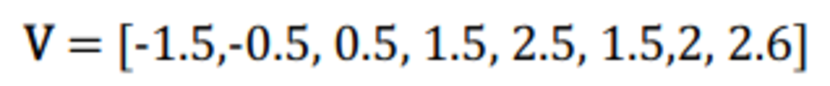
(a) PAA

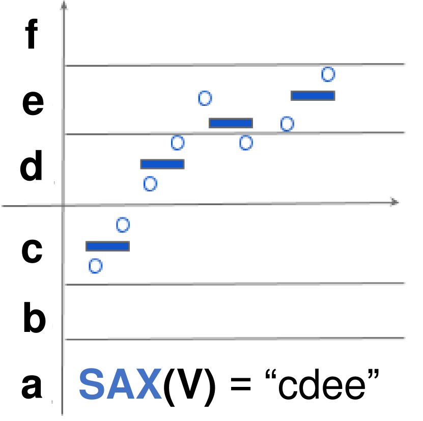
(b) iSAX

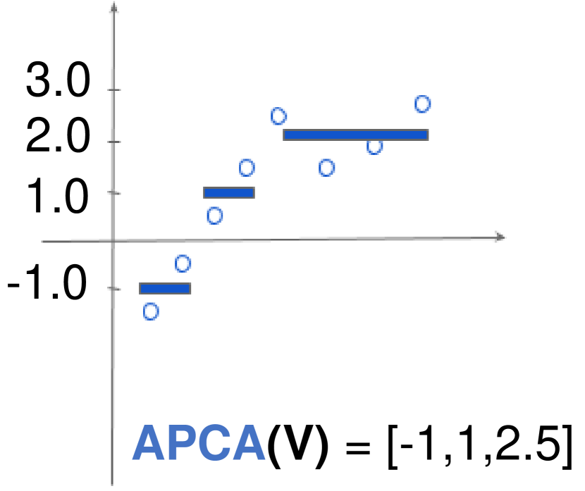
(c) APCA

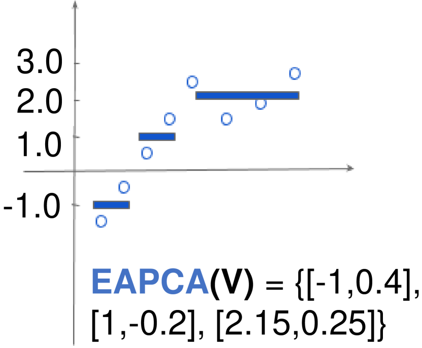
(d) EAPCA

Figure 1. Summarization Techniques

Similarity Search Methods. Exact similarity search methods are either sequential or index-based. The former compare a query series to each candidate series in the dataset, whereas the latter limit the number of such comparisons using efficient data structures and algorithms. An index is built using a summarization technique that supports lower-bounding (Faloutsos et al., 1994). During search, a filtering step exploits the index to eliminate candidates in the summarized space with no false dismissals, and a refinement step verifies the remaining candidates against the query in the original high-dimensional space (Ciaccia et al., 1997; Ferhatosmanoglu et al., 2000; Camerra et al., 2010; Zoumpatianos et al., 2016; Schäfer and Högqvist, 2012; Wang et al., 2013; Beckmann et al., 1990; Yagoubi et al., 2020; Linardi and Palpanas, 2018; Echihabi et al., 2021a, c, 2020a). We describe below the state-of-the-art exact similarity search techniques (Echihabi et al., 2018). Note that the scope of this paper is single-node systems, thus, we do not cover distributed approaches such as TARDIS (Zhang et al., 2019) and DPiSAX (Yagoubi et al., 2020).

The UCR Suite (Rakthanmanon et al., 2012) is an optimized sequential scan algorithm supporting the DTW and Euclidean distances for exact subsequence matching. We adapted the original algorithm to support exact whole matching, used the optimizations relevant to the Euclidean distance (i.e., squared distances and early abandoning) , and developed a parallel version, called PSCAN, that exploits SIMD, multithreading and double buffering.

The VA+file (Ferhatosmanoglu et al., 2000) is a skip-sequential index that exploits a filter file containing quantization-based approximations of the high dimensional data. We refer to the VA+file variant proposed in (Echihabi et al., 2018), which exploits DFT (instead of the Karhunen–Loève Transform) for efficiency purposes (Maccone, 2007).

The DSTree (Wang et al., 2013) is a tree-based approach which uses the EAPCA segmentation. The DSTree intertwines segmentation and indexing, building an unbalanced binary tree. Internal nodes contain statistics about the data series belonging to the subtree rooted at it, and each leaf node is associated with a file on disk that stores the raw data series. The data series in a given node are all segmented using the same policy, but each node has its own segmentation policy, which may result in nodes having a different number of segments or segments of different lengths. During search, it exploits the lower-bounding distance $\mathrm{LB_{EAPCA}}$ to prune the search space. This distance is calculated using the EAPCA summarization of the query and the synopsis of the node, which refers to the EAPCA summaries of all series that belong to the node.

ParIS+ (Peng et al., 2021c) is the first data series index for data series similarity search to exploit multi-core and multi-socket architectures. It is a tree-based index belonging to the iSAX family (Palpanas, 2020). Its index tree is comprised of several root subtrees, where each subtree is built by a single thread and a single thread can build multiple subtrees. During search, ParIS+ implements a parallel version of the ADS+ SIMS algorithm (Zoumpatianos et al., 2016), which prunes the search space using the iSAX summarizations and the lower-bounding distance $\mathrm{LB_{SAX}}$.

Hercules vs. Related Work. Hercules exploits the data-adaptive EAPCA segmentation proposed by DSTree (Wang et al., 2013) to cluster similar data series in the same leaf. This results in a binary tree which cannot be efficiently constructed and processed by utilizing the simple parallelization techniques of ParIS+ (Peng et al., 2021c). Specifically, the parallelization strategies of the index construction and query answering algorithms of ParIS+ exploit the large fanout of the root node, such that threads do not need to synchronize access to the different root subtrees. However, in Hercules, threads need to synchronize from the root level. Therefore, Hercules uses a novel parallel index construction algorithm to build the tree.

In addition, unlike previous work, Hercules stores the raw data series belonging to the leaves using a two-level buffer management architecture. This scheme plays a major role in achieving the good performance exhibited by Hercules, but results in the additional complication of having to cope with the periodic flushing of HBuffer to the disk. This flushing is performed by a single thread (the flush coordinator) to maintain I/O cost low. Additional synchronization is required to properly manage all threads that populate the tree, until flushing is complete. Note also that ParIS+ builds the index tree based on iSAX, thus, it only accesses the raw data once to calculate the iSAX summaries and insert the latter into the index tree. Node splits are also based on the summaries, which fit in-memory. However, Hercules builds the index tree using the disk-based raw data, making the index construction parallelization more challenging. Finally, ParIS+ treats all queries in the same way, whereas Hercules adapts its query answering strategy to each query.

Our experiments (Section 4) demonstrate that Hercules outperforms on query answering both DSTree and ParIS+ by up to 1-2 orders of magnitude across all query workloads.

3. The Hercules Approach

3.1. Overview

The Hercules pipeline consists of two main stages: an index construction stage, where the index tree is built and materialized to disk, and a query answering stage where the index is used to answer similarity search queries.

The index construction stage involves index building and index writing. During index building, the raw series are read from disk and inserted into the appropriate leaf of the Hercules EAPCA-based index tree. As their synopses are required only for query answering, to avoid contention at the internal nodes, we update only the synopses of the leaf nodes during this phase, while the synopses of the internal nodes are updated during the index writing phase. The raw series belonging to all the leaf nodes are stored in a pre-allocated memory buffer called HBuffer. Once all the data series are processed, index construction proceeds to index writing: the leaf nodes are post-processed to update their ancestors’ synopses, and the iSAX summaries are calculated. Moreover, the index is materialized to disk into three files: (i) HTree, containing the index tree; (ii) LRDFile, containing the raw data series; and (iii) LSDFile containing their iSAX summaries (in the same order as LRDFile’s raw data).

Hercules’s query answering stage consists of four main phases: (1) The index tree is searched heuristically to find initial approximate answers. (2) The index tree is pruned based on these initial answers and the EAPCA lower-bounding distances in order to build the list of candidate leaves (LCList). If the size of LCList is large (EAPCA-based pruning was not effective), a single-thread skip-sequential search on LRDFile is preferred (so phases 3 and 4 are skipped). (3) Additional pruning is performed by multiple threads based on the iSAX summarizations of the data series in the candidate leaves of LCList. The remaining data series are stored in SCList. If the size of SCList is large (SAX-based pruning was low), a skip-sequential search using one thread is performed directly on LRDFile and phase 4 is skipped. (4) Multiple threads calculate real distances between the query and the series in SCList, and the series with the lowest distances are returned as final answers. Thus, Hercules prunes the search space using both the lower-bounding distances $\mathrm{LB_{EAPCA}}$ (Wang et al., 2013) and $\mathrm{LB_{SAX}}$ (Lin et al., 2003).

3.2. The Hercules Tree

Figure 2 depicts the Hercules tree. Each node $\mathcal{N}$ contains: (i) the size, $\rho$, of the set $\mathbb{S}_{\mathcal{N}}=\{S_{1},\dots,S_{\rho}\}$ of all series stored in the leaf descendants of $\mathcal{N}$ (or in $\mathcal{N}$ if it is a leaf); (ii) the segmentation $SG=\{r_{1},...,r_{m}\}$ of $\mathcal{N}$, where $r_{i}$ is the right endpoint of $SG_{i}$, the $i$th segment of $SG$, with $1\leq i\leq m$, $1\leq r_{1}<...<r_{m}=n$, $r_{0}=0$ and $n$ is the length of the series; and (iii) a synopsis $Z=(z_{1},z_{2},...,z_{m})$, where $z_{i}=\{\mu_{i}^{min},\mu_{i}^{max},\sigma_{i}^{min},\sigma_{i}^{max}\}$ is the synopsis of the segment $SG_{i}$, $\mu_{i}^{min}=min(\mu_{i}^{S_{1}},\dots,\mu_{i}^{S_{\rho}})$, $\mu_{i}^{max}=max(\mu_{i}^{S_{1}},\dots,\mu_{i}^{S_{\rho}})$, $\sigma_{i}^{min}=min(\sigma_{i}^{S_{1}},\dots,\sigma_{i}^{S_{\rho}})$, and $\sigma_{i}^{max}=max(\sigma_{i}^{S_{1}},\dots,\sigma_{i}^{S_{\rho}})$.

A leaf node is associated with a FilePosition which indicates the position of the leaf’s raw data in LRDFile and that of the leaf’s iSAX summaries in LSDFile. An internal node contains pointers to its children nodes and a splitting policy. When a leaf node $\mathcal{N}$ exceeds its capacity $\tau$ (leaf threshold), it is split into two children nodes $N_{l}$ and $N_{r}$, which are leaf nodes, and $\mathcal{N}$ becomes an internal node.

Hercules exploits a splitting policy that (similarly to DSTree) allows the resolution of a node’s summarization to increase along two dimensions: horizontally (H-split) and vertically (V-split), unlike the other data series indexes (Camerra et al., 2014; Zoumpatianos et al., 2016; Schäfer and Högqvist, 2012), which allow either one or the other (for example, iSAX-based indexes only allow horizontal splitting). A node $\mathcal{N}$ is split by picking $SG_{i}$, one of the $m$ segments of $\mathcal{N}$, and using the mean (or the standard deviation) of the points belonging to $SG_{i}$ to redistribute the series in $\mathbb{S}_{N}$ among $N_{l}$ and $N_{r}$. In an H-split, both $N_{l}$ and $N_{r}$ have the same segmentation as $\mathcal{N}$ whereas in a V-split, the children nodes have one additional segment. In an H-split using the mean, the data series in $\mathbb{S}_{N}$ which have a mean value for segment $SG_{i}$ in the range [$\mu_{i}^{min},(\mu_{i}^{min}+\mu_{i}^{max})/2$) will be stored in $N_{l}$ and those whose range is in [$(\mu_{i}^{min}+\mu_{i}^{max})/2,\mu_{i}^{max}$] will be stored in $N_{r}$. An H-split using the standard deviation proceeds in the same fashion we just described, except it uses the values of standard deviations instead of mean values. A V-split first splits $SG_{i}$ into two new segments then applies an H-split on one of them. For example, in Figure 2, node $\mathrm{I_{2}}$ has an additional segment compared to its parent $\mathrm{I_{1}}$, because it was split vertically, while the latter has the same segmentation as Root, because it was split horizontally. If we suppose that $\mathrm{I_{1}}$ was split using mean values, the data series that were originally stored in $\mathrm{\mathbb{S}_{I_{1}}}$ are now stored in $\mathrm{\mathbb{S}_{L_{1}}}$ if their mean value $\mu_{1}<-0.075$ ($\frac{-0.25+0.10}{2}=-0.075$ ), and to its right child otherwise.

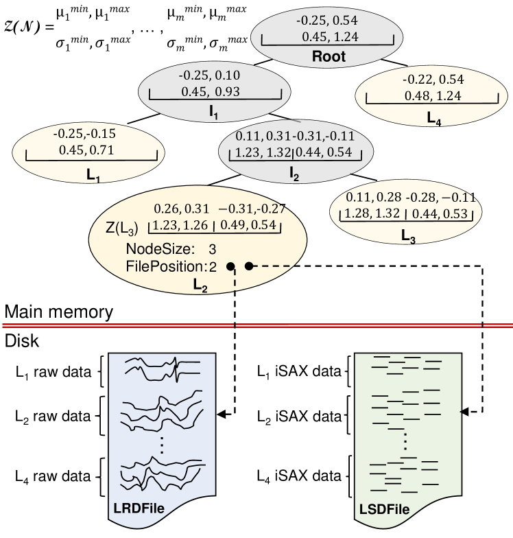
Figure 2. The Hercules Index Tree

3.3. Index Construction

3.3.1. Overview

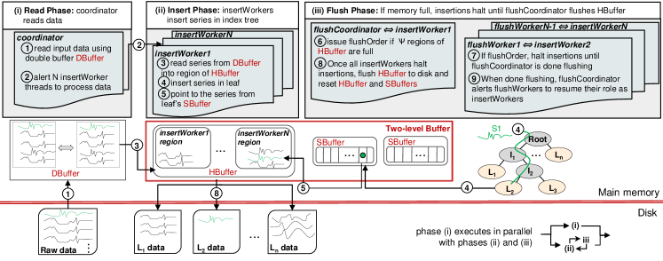
Figure 3. Hercules Index Building Workflow

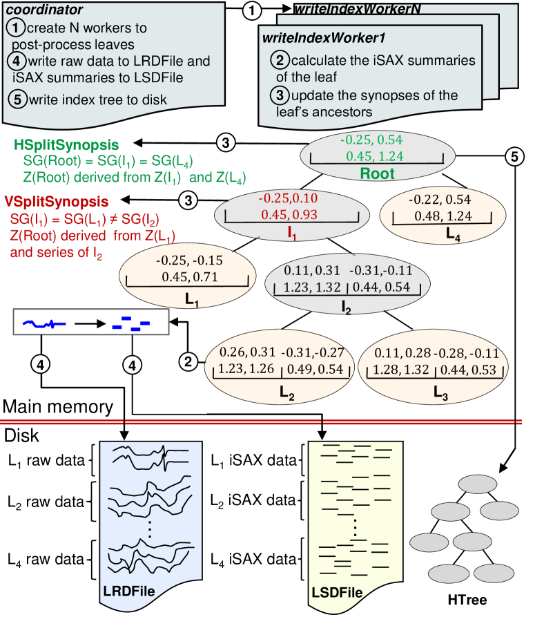
Figure 4. Hercules Index Writing Workflow

Figure 3 describes the index building workflow. Index building consists of three phases: (i) a read phase, (ii) an insert phase, and (iii) a flush phase. A thread acting as the coordinator and a number of InsertWorker threads operate on the raw data using a double buffer scheme, called DBuffer. Hercules leverages DBuffer to interleave the I/O cost of reading raw series from disk with CPU-intensive insertions into the index tree. The numbered circles in Figure 3 denote the tasks performed by the threads.

During the read phase, the coordinator loads the dataset into memory in batches, reading a batch of series from the original file into the first part of DBuffer (1). It gives up the first part of DBuffer when it is full and continues storing data into the second part (2).

During the insert phase, The InsertWorker threads read series from the part of the buffer that the coordinator does not work on (3) and insert them into the tree. Each InsertWorker traverses the index tree to find the appropriate leaf, routing left or right depending on the split policy of the visited node (4). Each tree leaf points to an SBuffer, an array of pointers to the raw data stored in HBuffer (5). We chose this architecture for performance reasons. Experiments showed that allocating a large memory buffer (HBuffer) at the start of the index creation and releasing it once all series have been inserted is more efficient than having each leaf pre-allocate its own memory buffer and release it when it is split, especially during the beginning of index construction where splits occur frequently. Our design results in a small number of system calls and reduces the occurrences of out-of-memory management issues (when a program issues a large number of memory cleanup operations, the memory can be retained by the process for later reuse).

Each InsertWorker has its own region in HBuffer and records the data series that it inserts there. When the number of full regions reaches a flush threshold, the flush phase starts (6), where the data in HBuffer is flushed to disk. This is achieved by identifying one of the InsertWorkers as the FlushCoordinator to undertake the task of flushing. The rest of the InsertWorkers wait until the FlushCoordinator is done (7). Careful synchronization is necessary between the FlushCoordinator and the rest of the InsertWorkers, which now play the role of the FlushWorkers. The FlushWorkers have to inform the FlushCoordinator when their region becomes full and synchronize with it to temporarily halt their execution (8) and resume it again after the flush phase completes (9).

Figure 4 describes the workflow of the index writing phase, which calculates in parallel the iSAX summaries and synopses of the internal nodes (1-3), and materializes HTree, LRDFile and LSDFile (4-5). Hercules stores the raw data series in LRDFile, as they are traversed in the tree leaves during an inorder traversal. To improve the pruning degree, it also calculates iSAX summaries for the data series and stores them in an array in memory. At the end of every execution, it flushes this array into LSDFile, to avoid recalculating them during query answering. LSDFile follows the same order as LRDFile. If HBuffer can hold the full dataset, these operations do not require any disk access.

3.3.2. Index Building Algorithms

We start by providing the details of Algorithm 1 which is executed by the coordinator. After the coordinator fills in the first part of DBuffer (line 1), it spawns the InsertWorkers (line 1). While the InsertWorkers process the data in one part of DBuffer, the coordinator fills in the other part of the buffer, by reading data series from disk in chunks of size $DBSize$ (lines 1-1). A $Toggle$ bit is used by the coordinator to alternate working on the two parts of DBuffer (line 1). Before starting to refill a part of DBuffer, the coordinator has to wait for all InsertWorkers to finish processing the data series in it. This is achieved using the DBarrier (line 1). DBarrier is a Barrier object (line 1, Algorithm 1), i.e., it is an instance of an algorithm that forces asynchronous threads to reach a point of synchronization: when a thread reaches a Barrier object, it is blocked until all threads that are supposed to reach the Barrier object have done so. Once all the data has been processed, the coordinator sets the Finished[Toggle] flag and waits for all InsertWorkers to finish their work (lines 1-1). As the coordinator always works in the part of the buffer that the workers will process next, it has to enter the barrier one more time (line 1) after it sets the Finished[Toggle] flag.

Input: File* File, Index* Idx, Integer NumThreads, Integer DataSize

1 Integer NumInsertWorkers $\leftarrow$ NumThreads-1;

2 Barrier DBarrier for NumThreads threads;

3 Barrier ContinueBarrier for NumInsertWorkers threads;

4 Barrier FlushBarrier for NumInsertWorkers threads;

5 Shared Integer InitialDBSize;

6 Shared Integer DBSize[2] $\leftarrow$ $\{0,0\}$;

7 Shared Integer DBCounter[2] $\leftarrow$ $\{0,0\}$;

8 Shared Boolean FlushCounter $\leftarrow$ FALSE;

9 Shared Boolean FlushOrder $\leftarrow$ FALSE;

10 Shared Boolean Finished[2] $\leftarrow$ $\{$FALSE, FALSE$\}$;

11 Shared Thread Workers[NumInsertWorkers];

12 initialize Workers;

13 Static Bit Toggle $\leftarrow 0$;

14 DBSize[Toggle] $\leftarrow$ min{InitialDBSize, DataSize};

15 read DBSize[Toggle] data series from file into DBuffer[Toggle] of Idx;

16 Toggle $\leftarrow$ 1-Toggle;

17 for j $\leftarrow$ 0 to NumInsertWorkers do

18       each Worker in Workers runs an instance of InsertWorker(Idx);

19      

20for i $\leftarrow$ DBSize[1-Toggle]; i $<$ DataSize; i+=DBSize[Toggle] do

21       DBSize[Toggle] $\leftarrow$ min{InitialDBSize, DataSize-i};

22       read DBSize[Toggle] data series from file into DBuffer[Toggle] of Idx;

23       DBCounter[Toggle] $\leftarrow$ $0$;

24       Toggle $\leftarrow$ 1-Toggle;

25       Coordinator reaches DBarrier;

26      

27Finished[Toggle] $\leftarrow$ TRUE;

28 Coordinator reaches DBarrier;

29

30wait for all the InsertWorkers to finish;

31

Algorithm 1 BuildHerculesIndex

Input: Index* Idx

1 Node Root $\leftarrow$ Root of Idx;

2 Bit Toggle $\leftarrow$ $0$;

3 Integer Pos $\leftarrow$ $0$;

4 Float* S_raw;

5

6 while !Finished[Toggle] do

7       if InsertWorker’s buffer has at least DBSize[Toggle] empty slots then

8             Pos $\leftarrow$ FetchAdd(DBCounter[Toggle], 1);

9             while (Pos $<$ DBSize[Toggle]) do

10                   S_raw $\leftarrow$ DBuffer[Toggle][Pos];

11                   InsertSeriesToNode(Idx, Root, S_raw);

12                   Pos $\leftarrow$ FetchAdd(DBCounter[Toggle], 1);

13                  

14       InsertWorker blocks on DBarrier;

15       if InsertWorker is FlushCoordinator then

16             FlushCoordinator(Idx);

17            

18      else

19             FlushWorker();

20            

21      Toggle $\leftarrow$ 1-Toggle;

22      

Algorithm 2 InsertWorker

Input: Index* Idx

1 Integer Volatile Cnt;

2 Integer Tmp;

3 Workers[WorkerID].ContinueHandShake $\leftarrow$ TRUE;

4 for each Worker in Workers do

5       while !Worker.ContinueHandShake do

6             for Tmp $\leftarrow$ 0; Tmp $<$ BUSYWAIT; Tmp++ do

7                   Cnt++;

8 if (FlushCoordinator’s region in HBuffer is full) OR (FlushCounter $>=$ FLUSH_THRESHOLD) then

9       FlushOrder $\leftarrow$ TRUE;

10      

11FlushCounter $\leftarrow 0$;

12 FlushCoordinator blocks on ContinueBarrier;

13 Workers[WorkerID].ContinueHandShake $\leftarrow$ FALSE;

14 if FlushOrder then

15       materialize to disk the data in Idx’s leaves and reset soft and hard buffers;

16       FlushOrder $\leftarrow$ FALSE ;

17       FlushCoordinator blocks on FlushBarrier;

18      

Algorithm 3 FlushCoordinator

1 $\triangleright$ a worker’s buffer is full if it cannot hold at least DBSize[InitialDBSize] series;

2 if FlushWorker’s region in HBuffer is full then

3       FetchAdd(FlushCounter, 1);

4      

5Workers[WorkerID].ContinueHandShake $\leftarrow$ TRUE;

6 FlushWorker blocks on ContinueBarrier;

7 Workers[WorkerID].ContinueHandShake $\leftarrow$ FALSE;

8 if FlushOrder then

9       FlushWorker blocks on FlushBarrier;

10      

Algorithm 4 FlushWorker

Each InsertWorker executes Algorithm 2. The execution alternates between insertion phases, where all InsertWorkers insert data series in the tree, and flushing phases where the first of the InsertWorkers (that plays the role of FlushCoordinator) flushes all buffers to disk, while the other FlushWorkers block waiting for FlushCoordinator to complete the flushing phase. InsertWorkers keep track of the part of DBuffer they work on in the variable $Toggle$.

In Algorithm 2, each InsertWorker first checks if it has enough space in HBuffer to store at least $DBSize$ series (lines 2-2). Next, the InsertWorker reads a data series from DBuffer[Toggle] (line 2) and calls InsertSeriesToNode to insert this data series in the index tree. To synchronize reads from DBuffer[Toggle], InsertWorkers use a FetchAdd variable DBCounter[Toggle]. DBCounter[Toggle] is incremented on line 2 and it is reset to $0$ by the coordinator (line 1 in Algorithm 1). To synchronize with the coordinator, InsertWorkers reach the DBarrier once they have finished processing the data in the current part of DBuffer, or have exhausted their capacity in HBuffer (line 2).

To execute the flushing protocol, the FlushCoordinator executes an instance of Algorithm 3, whereas FlushWorkers execute an instance of Algorithm 4. The FlushCoordinator and FlushWorkers synchronize using the ContinueHandShake bits, the ContinueBarrier and the FlushBarrier. The FlushCoordinator reads the FlushCounter to determine the number of FlushWorkers that have exceeded the capacity of their regions in HBuffer (for loop at line 3). Each InsertWorker uses the ContinueHandShake bit to notify the coordinator if its part in HBuffer is full, in which case it increments FlushCounter. The FlushCoordinator waits until it sees that all these bits are set (lines 3-3). If the FlushCounter reaches a threshold, or the FlushCoordinator itself is full, FlushOrder is set to TRUE (line 3). The FlushCoordinator waits at the ContinueBarrier to let FlushWorkers know that it has made its decision and resets its own ContinueHandShake bit to FALSE. If FlushOrder is TRUE, it flushes the raw data in HBuffer to disk, resets the SBuffer pointers in the leaves, and resets FlushCounter to zero and FlushOrder to FALSE. The FlushCoordinator informs FlushWorkers that it has finished the flushing by reaching the FlushBarrier.

In Algorithm 4, FlushWorkers increase the FetchAdd variable FlushCounter if their region in HBuffer is full (line 4) and flip the ContinueHandShake bit to TRUE (line 4). FlushWorkers need to wait until the FlushCoordinator has received all handshakes and issued the order to flush or continue insertions, before they reach the ContinueBarrier (lines 4). The ContinueHandShake is then set back to FALSE (line 4). If the FlushCoordinator has set FlushOrder to TRUE, FlushWorkers wait at the FlushBarrier (line 4).

Input: Index* Idx, Node* $\scriptstyle\mathcal{N}$, Float* S_raw

1 $\scriptstyle\mathcal{N}$ $\leftarrow$ RouteToLeaf($\mathcal{N}$, S_raw);

2 acquire lock on $\scriptstyle\mathcal{N}$;

3 while not $\scriptstyle\mathcal{N}$.IsLeaf do

4       release lock on $\scriptstyle\mathcal{N}$;

5       $\scriptstyle\mathcal{N}$ $\leftarrow$ RouteToLeaf($\scriptstyle\mathcal{N}$, S_raw);

6       acquire lock on $\scriptstyle\mathcal{N}$;

7      

8 update the synopsis of $\scriptstyle\mathcal{N}$ using S_raw;

9 add S_raw in this thread’s region of HBuffer and a pointer to it in $\scriptstyle\mathcal{N}$’s SBuffer;

10 if $\scriptstyle\mathcal{N}$ is full then

11       Policy $\leftarrow$ getBestSplitPolicy($\scriptstyle\mathcal{N}$);

12       create two children nodes for $\scriptstyle\mathcal{N}$ according to Policy;

13       get all data series in $\scriptstyle\mathcal{N}$ from memory and disk (if flushed);

14       distribute data series among the two children nodes and update the node synopses accordingly;

15       $\scriptstyle\mathcal{N}$.IsLeaf $\leftarrow$ FALSE;

16      

17release lock on $\scriptstyle\mathcal{N}$;

Algorithm 5 InsertSeriesToNode

Algorithm 5 describes the steps taken by each thread to insert one data series into the index. First, the thread traverses the current index tree to find the correct leaf to insert the new data series (line 5), then it attempts to acquire a lock on the leaf node (line 5). Another thread that has already acquired a lock on this same leaf might have split the node; therefore, it is important to verify that the node is still a leaf before appending data to it. Once a leaf is reached, its synopsis is updated with the data series statistics (line 5) and the latter is appended to it (line 5). The lock on the leaf is then released (line 5). In the special case when a leaf node reaches its maximum capacity (line 5), the best splitting policy is determined following the same heuristics as in the DSTree (Wang et al., 2013) (line 5) and the node is split by creating two new children nodes (line 5). The series in the split node are fetched from memory and disk (if they have been flushed to disk), then redistributed among the left and right children nodes according to the node’s splitting policy. Once all series have been stored in the correct leaf, the split node becomes an internal node (line 5).

3.3.3. Index Writing Algorithms

We now describe the algorithms used in the index writing phase which materializes the index tree and the raw data. This phase also updates the synopsis of the internal nodes and calculates the iSAX summaries of the raw data series (which are also materialized).

Input: Index* Idx, File* File, Integer NumThreads

1 Shared Integer LeafCounter $\leftarrow$ 0;

2 write Idx.Settings to File;

3 for j $\leftarrow$ 0 to NumThreads-1 do

4       create a thread to execute an instance of WriteIndexWorker(Idx, LeafCounter);

5      

6 WriteLeafData(Idx);

7 for j $\leftarrow$ 0 to NumThreads-1 do

8       wait until all WriteIndexWorker threads are done;

9 WriteIndexTree(Idx, Idx.Root, File);

Algorithm 6 WriteHerculesIndex

Algorithm 6 which implements this phase is invoked by a thread called the WriteIndexCoordinator. The coordinator first saves the index settings used to build the index which include the data series length, the dataset size, and the leaf threshold (line 6). Recall that for performance reasons, the synopses of the internal nodes were not updated during index building (Algorithm 5). The WriteIndexCoordinator creates a number of workers (WriteIndexWorkers) to concurrently update these synopses and to calculate the iSAX summaries of the raw data series. At the same time, the WriteIndexCoordinator calls WriteLeafData to materialize the data contained in the leaves that have been fully processed by the WriteIndexWorkers. After all WriteIndexWorkers are done, the coordinator calls WriteIndexTree to materialize the data of the internal nodes.

Each WriteIndexWorker (Algorithm 7) processes one leaf at a time, calculating the iSAX summaries of the leaf’s raw data and updating the synopses of its ancestor nodes (line 7). Then, it notifies the WriteIndexCoordinator that it completed processing this leaf (line 7). Once all leaves have been processed, the worker terminates.

Input: Index* Idx, Shared Integer LeafCounter

1 Integer $j$ $\leftarrow$ 0;

2 Node $\scriptstyle\mathcal{L}$;

3 $j\leftarrow$ FetchAdd(LeafCounter, 1);

4 $\scriptstyle\mathcal{L}\leftarrow$ jth leaf of the index tree (based on inorder traversal);

5 while j ¡ Idx.NumLeaves do

6       ProcessLeaf(Idx,$\scriptstyle\mathcal{L}$);

7       $\scriptstyle\mathcal{L}$.processed $\leftarrow$ TRUE;

8       wait until $\scriptstyle\mathcal{L}$.written is equal to TRUE;

9       j $\leftarrow$ FetchAdd(LeafCounter, 1);

10      

Algorithm 7 WriteIndexWorker

For each processed leaf of the index tree, WriteLeafData simply stores the leaf’s raw data and their iSAX summaries into two disk files, called LRDFile and LSDFile, respectively.

We next discuss the post-processing of each individual leaf $\mathcal{L}$, which consists mainly of the calculation of the iSAX summaries of the data series belonging in $\mathcal{L}$ and the update of the synopses of the ancestors of $\mathcal{L}$. Recall that the synopsis of a node $\mathcal{N}$ consists of the synopses of all segments in $\mathcal{N}$’s segmentation, where each segment is represented using the minimum/maximum mean and standard deviation of all points within this segment among all series that traversed $\mathcal{N}$. Therefore, updating the synopsis of an internal node $\mathcal{N}$ requires updating the synopses of all its segments. The operations required to do so depend on the type of the split that the node $\mathcal{N}$ has undergone. If a node has been split vertically, the synopsis of the segment that was vertically split is calculated gradually by repeatedly calling VSplitSynopsis (Algorithm 8) on each raw data series, whereas the synopsis of its other segments can be derived from those of its children nodes by calling HSplitSynopsis (Algorithm 9). So HSplitSynopsis is invoked only once for each leaf node.

Input: Node $\scriptstyle\mathcal{N}$, Float * S_raw

1 Segment SG;

2 while $\scriptstyle\mathcal{N}$ is not null do

3       if $\scriptstyle\mathcal{N}$ has a split vertical segment  then

4             SG $\leftarrow$ the split segment of $\scriptstyle\mathcal{N}$;

5             S_sketch $\leftarrow$ CalcMeanSD(S_raw, SG_start, SG_end);

6             acquire lock on $\scriptstyle\mathcal{N}$;

7             update the min/max mean and sd of SG with S_sketch.Mean and S_sketch.SD;

8             release lock on $\scriptstyle\mathcal{N}$;

9            

10      $\scriptstyle\mathcal{N}$ $\leftarrow$ $\scriptstyle\mathcal{N}$.Parent;

11      

Algorithm 8 VSplitSynopsis

Input: Node $\scriptstyle\mathcal{N}$

1 Segment SG_p, Node $\scriptstyle\mathcal{P}$ ;

2 $\scriptstyle\mathcal{P}$ $\leftarrow$ $\scriptstyle\mathcal{N}$.Parent;

3

4while $\scriptstyle\mathcal{P}$ is not null do

5       for each non vertically split segment SG_p in $\scriptstyle\mathcal{P}$ do

6             SG_n $\leftarrow$ the corresponding segment of SG in $\scriptstyle\mathcal{N}$;

7             acquire lock on $\scriptstyle\mathcal{N}$;

8             update the min/max mean and sd of SG_p with the min/max mean and sd of SG_n ;

9             release lock on $\scriptstyle\mathcal{N}$;

10            

11      $\scriptstyle\mathcal{N}$ $\leftarrow$$\scriptstyle\mathcal{P}$;

12       $\scriptstyle\mathcal{P}$ $\leftarrow$ $\scriptstyle\mathcal{N}$.Parent;

13      

Algorithm 9 HSplitSynopsis

In the case of a horizontal split, the synopsis of $\mathcal{N}$ can be derived entirely from those of its children (Algorithm 9).

Routine WriteIndexTree materializes the tree nodes. It applies a recursive (Postorder) tree traversal, updating the size of each node and writing the node’s data into $File$.

3.4. Query Answering

3.4.1. Overview

Figure 5 describes query answering in Hercules, which consists of four main steps. The first and second steps are run sequentially, whereas the others are run in parallel. The distance calculations in all steps are performed using SIMD.

In the first step, when a kNN query $S_{Q}$ arrives, the index tree is traversed to visit at most $\mathrm{{L_{max}}}$ leaves. When a leaf $\mathcal{L}$ is visited, the series that belong to it are read from LRDFile and the Euclidean distance (ED) between $S_{Q}$ and every series in $\mathcal{L}$ is calculated. The $k$ best-so-far neighbors, i.e., the $k$ series with the smallest Euclidean distances to $S_{Q}$, are stored in array $Results$. The leaves are chosen based on a priority queue $PQ$, which initially contains just the index tree Root node. The algorithm iteratively removes a node $\mathcal{N}$ from the priority queue, and if the $\mathrm{LB_{EAPCA}}$ distance of $S_{Q}$ to $\mathcal{N}$ is larger than the current value of $\mathrm{BSF_{k}}$, the $k^{th}$ smallest ED distance in $Results$, the node is pruned. Otherwise, if $\mathcal{N}$ is a leaf, it is added to $PQ$, and if it is an internal node, its children are added to $PQ$ if their $\mathrm{LB_{EAPCA}}$ distance to $S_{Q}$ is smaller than $\mathrm{BSF_{k}}$. Once $\mathrm{{L_{max}}}$ leaves are visited, the first step terminates returning the array $Results$ with $k$ initial answers. This step is called approximate search.

The second step takes place entirely in-memory with no ED distance calculations, thus, the current $\mathrm{BSF_{k}}$ is not updated. This step resumes processing $PQ$ as in step one, except when a leaf is visited: it is either pruned, based on $\mathrm{BSF_{k}}$, or added to a list of candidate leaves, called LCList, in increasing order of the leaves file positions in LRDFile. If the pruning is smaller than a threshold, EAPCA_TH, a skip-sequential scan is performed on LRDFile and the final results are stored in $Results$. The skip-sequential scan seeks the file position of the first leaf in LCList, calculates the ED distances between the data in this leaf and $S_{Q}$ and updates $Results$ if applicable. Similarly, subsequent leaves are processed in the order they appear in LCList, provided they cannot be pruned using $\mathrm{BSF_{k}}$.

If the size of LCList is relatively small, Hercules proceeds to the third step, also entirely in-memory. Threads process LCList in parallel. Each thread picks a leaf $\mathcal{L}$ from LCList, loads the iSAX summaries of $\mathcal{L}$’s data series from LSDFile, which is pre-loaded with the index tree, and calculates the $\mathrm{LB_{SAX}}$ distance between $S_{Q}$ and each iSAX summary. If the iSAX summary cannot be pruned, the file position of the series and its $\mathrm{LB_{SAX}}$ distance are added to SCList. Note that the file position of a series in LRDFile is the same as that of its iSAX summary in LSDFile. This step terminates once all the leaves in LCList are processed. If the pruning is smaller than a threshold, SAX_TH, one thread performs a skip-sequential scan on LRDFile and the final results are stored in $Results$.

Note that a skip-sequential scan on LRDFile is favored when pruning is low for efficiency. It incurs as many random I/O operations as the number of non pruned leaves, whereas applying the second filtering step using $\mathrm{LB_{SAX}}$ on a large number of series incurs as many random I/O operations as the number of non-pruned series. The EAPCA_TH and SAX_TH thresholds are tuned experimentally, and exhibit a stable behavior (cf. Section 4).

If the size of SCList is relatively small, Hercules proceeds to the fourth step, which computes the final results based on SCList and LRDFile. Multiple threads process SCList in parallel. Each thread picks a series from SCList and compares its $\mathrm{LB_{SAX}}$ against the current $\mathrm{BSF_{k}}$. If the series cannot be pruned, the thread loads the series corresponding to this summary from LRDFile, and calculates the Euclidean distance between this series and $S_{Q}$, updating $Results$ when appropriate. Once SCList has been processed entirely, the final answers are returned in $Results$.

3.4.2. Query Answering Algorithms

Algorithm 10 outlines the $k$NN exact nearest neighbor search with Hercules. It takes as arguments, the query series $S_{Q}$, the index $Idx$, a threshold which determines the maximum number of leaves, $L_{max}$, that can be visited during the approximate search, the number $k$ of neighbors to return, and two thresholds, EAPCA_TH and SAX_TH, which determine whether multi-threading will be used (and will be discussed later).

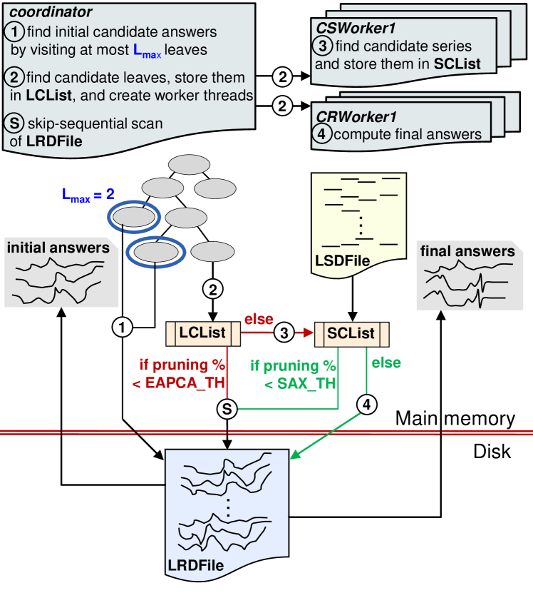
Figure 5. Query Answering Workflow

Input: Query S_Q, Index* Idx, Integer L_max, Integer k, Float EAPCA_TH, Float SAX_TH

1 Priority queue PQ; $\triangleright$ initially empty

2 Array Results containing k structs of type Result with fields Dist and Pos each; $\triangleright$ initially, each array element stores $\langle\infty$, NULL $\rangle$

3 Float BSF_k;

4 Float eapca_pr, sax_pr;

5 List* LCList, SCList;

6 Approx-kNN(S_Q, Idx, PQ, L_max, k, Results);

7 BSF_k $\leftarrow$ Results[k-1].Dist;

8 FindCandidateLeaves(S_Q, Idx, PQ, BSF_k, LCList);

9 eapca_pr $\leftarrow$ 1-size(LCList)/(total leaves of index tree);

10

11if eapca_pr ¡ EAPCA_TH then

12       perform a skip-sequential scan on Idx.LRDFile and update Results;

13      

14else

15       FindCandidateSeries(S_Q, Idx, BSF_k, LCList, SCList);

16       sax_pr $\leftarrow$ 1-size(SCList)/(total series of Idx);

17       if sax_pr ¡ SAX_TH then

18             perform a skip-sequential scan on Idx.LRDFile;

19            

20      else

21             ComputeResults(S_Q, Idx, k, Results, SCList);

22            

23return Results;

Algorithm 10 Exact-kNN

The algorithm uses an array $Results$ to store the current $k$ best-so-far answers at each point in time, two array-lists, namely LCList and SCList, which hold the candidate leaves and series, respectively, and a priority queue $PQ$ in which the priority is based on the $\mathrm{LB_{EAPCA}}$ distance of the query to a given node (lines 10-10).

First, an approximate $k$NN search is performed by calling the function Approx-kNN, which stores in the array $Results$, the $k$ approximate neighbors for query $S_{Q}$ by visiting at most $\mathrm{{L_{max}}}$ leaves. The variable $\mathrm{BSF_{k}}$ is initialized with the real distance of the $k^{th}$ neighbor to $S_{Q}$ and is used by the FindCandidateLeaves function to prune the search space. The non-pruned leaves are stored in LCList (line 10). If the size of LCList is large enough (so that $eapca\_pr$ is smaller than the EAPCA_TH threshold), then a skip-sequential scan on LRDFile is performed using one thread and $Results$ is updated with the best answers (line 10).

Otherwise, FindCandidateSeries applies a second filter using the iSAX representation of the series belonging to the leaves in LCList using the $\mathrm{LB_{SAX}}$ distance, and stores the non-pruned candidate series in SCList (line 10). If the size of SCList is large, i.e., that the pruning based on $\mathrm{LB_{SAX}}$ is low, then a skip-sequential scan on LRDFile is performed using one thread (line 10). Otherwise, ComputeResults (line 10) loads the series in SCList from disk and calculates their real ED distance to the query returning the $k$ series with the minimum ED distance to $S_{Q}$ as the final answers. All real and lower-bounding distance calculations used exploit SIMD for efficiency (following (Peng et al., 2021c, a)).

The building blocks of Algorithm 10 are as follows.

Step 1: Finding Initial Approximate Answers. Algorithm 11 finds $k$ approximate first baseline answers and stores them in the array $Results$ in increasing order of the real Euclidean distance. It visits a maximum of $L_{max}$ leaves, where $L_{max}$ is a parameter provided by the user and is 1 by default. In line 11, it pops the element in $PQ$ with the highest priority, i.e., the node with the lowest $\mathrm{LB_{EAPCA}}$ to the query. To understand the reason behind allocating a higher priority to a smaller $\mathrm{LB_{EAPCA}}$, recall that $\mathrm{LB_{EAPCA}}$ is a lower-bounding distance. Therefore, if a popped node has an $\mathrm{LB_{EAPCA}}$ value greater than the current $\mathrm{BSF_{k}}$ answer, then search can terminate since any series in the subtree rooted at this node has a real distance that is greater than or equal to $\mathrm{LB_{EAPCA}}$, and thus cannot improve $\mathrm{BSF_{k}}$ (line 11). Besides, since the priority in $PQ$ is based on the minimum $\mathrm{LB_{EAPCA}}$, all remaining nodes in $PQ$ can be pruned because their lower-bounding distances will also be greater than $\mathrm{BSF_{k}}$. Note that we use SIMD operations to speed up the calculations of the $\mathrm{LB_{EAPCA}}$ distances.

Input: Query S_Q, Index* Idx, Priority Queue PQ, Integer L_max, Integer k, Result* Results

1 PQElement $q$ $\triangleright$ PQElement has two fields, $\scriptstyle\mathcal{N}$ and Dist;

2 Float RootLB_EAPCA $\leftarrow$ $\mathtt{CalculateLB_{EAPCA}}$(S_Q, Idx.Root);

3 Integer VisitedLeaves $\leftarrow$ $0$;

4 add Idx.Root to PQ with priority RootLB_EAPCA;

5 while VisitedLeaves ¡ L_max AND NOT IsEmpty(PQ) do

6       $\langle\scriptstyle\mathcal{N}$, LB_EAPCA $\rangle$ $\leftarrow$ DeleteMinPQ(PQ);

7       if LB_EAPCA $>$ BSF_k then

8             break;

9      if $\scriptstyle\mathcal{N}$ is a leaf then

10             for each S in $\scriptstyle\mathcal{N}$ do

11                   RealDist $\leftarrow$ CalculateRealDist(S_Q, S);

12                   if RealDist $<$ BSF_k then

13                         create new struct result of type Result;

14                         result.Dist $\leftarrow$ RealDist;

15                         result.Pos $\leftarrow$ Position of S in LRDFile;

16                         add result to Results;

17                         BSF_k $\leftarrow$ Results[k-1].Dist;

18                        

19            VisitedLeaves $\leftarrow$ VisitedLeaves+1;

20            

21      else

22             for each Child in $\scriptstyle\mathcal{N}$ do

23                   LB_EAPCA $\leftarrow$ CalculateLB_EAPCA(S_Q, Child);

24                   if LB_EAPCA $<$ BSF_k then

25                         add Child to PQ with priority LB_EAPCA;

Algorithm 11 Approx-kNN

If the non-pruned node is a leaf (line 11), then the series in this leaf are read from LRDFile, their real Euclidean distances to the query are calculated and the $Results$ array is updated if applicable (lines 11-11). The algorithm stops improving the $k$ answers once the leaves threshold is reached.

Instead, if the non-pruned node is an internal node (line 11), its children are added to $PQ$ if their $\mathrm{LB_{EAPCA}}$ is smaller than the current value of $\mathrm{BSF_{k}}$. Then the algorithm resumes processing the $PQ$ unless it is empty and stores the approximate $k$ answers in $Results$ to help the exact algorithm prune the search space.

Step 2: Finding Candidate Leaves.

Input: Query S_Q, Index* Idx, Priority queue PQ, Float BSF_k, List* LCList

1

2while NOT IsEmpty(PQ) do

3       $\langle\scriptstyle\mathcal{N}$, LB_EAPCA $\rangle$ $\leftarrow$ DeleteMin(PQ);

4       if LB_EAPCA $>$ BSF_k then

5             break;

6      if $\scriptstyle\mathcal{N}$ is a leaf then

7             add $\langle\scriptstyle\mathcal{N},{\it LB\textsubscript{EAPCA}}\rangle$ to LCList;

8            

9      else

10             for each Child in $\scriptstyle\mathcal{N}$ do

11                   LB_EAPCA $\leftarrow$ CalculateLB_EAPCA(S_Q,Child);

12                   if  LB_EAPCA $<$ BSF_k then

13                         add Child to PQ with priority LB_EAPCA;

14                        

15sort the leaves in LCList in increasing order of their position in the Idx.LRDFile;

Algorithm 12 FindCandidateLeaves

Once Algorithm 11 finds $k$ initial approximate answers, the ED distance between $S_{Q}$ and the $k^{th}$ answer, called $\mathrm{BSF_{k}}$, is used by Algorithm 12 to prune the search space and populate LCList with candidate leaves. Search in the index tree resumes with the remaining nodes in $PQ$ (line 12), i.e., nodes that were visited by algorithm 11 are not accessed again. If the current node’s $\mathrm{LB_{EAPCA}}$ is larger than the $\mathrm{BSF_{k}}$ distance, the algorithm terminates (line 12). Otherwise, it adds non-pruned leaves into LCList (line 12) and non-pruned internal nodes into the priority queue $PQ$ (lines 12-12). Note that leaves are treated differently in Algorithms 11 and 12: in the former, the series of the leaves are loaded from disk and the real distances are calculated between the series and the query, updating $Results$ as necessary, whereas in the latter, $Results$ is not updated and pointers to the leaves are stored for further processing, so the disk is not accessed in this case.

Once all nodes in $PQ$ have been processed, the candidate leaves in LCList are sorted in increasing order of their Position in LRDFile (line 12). This is to reduce the overhead of disk random I/O by ensuring that data pages are visited in the order that they are laid out on disk.

Step 3: Finding Candidate Series. While the previous building blocks of exact search use SIMD to efficiently calculate the real and lower-bounding distances, they run using a single thread. FindCandidateSeries is a multi-threaded algorithm that processes the candidate leaves in LCList to populate SCList with candidate data series. Each thread executes an instance of CSWorker. Once all threads have finished execution, the algorithm stores all candidate data series in SCList.

Input: Query S_Q, Char ** LSDFile, Float BSF_k, Integer id, List* LCList, List* SCList

1 Shared Integer LCL_Idx $\leftarrow$ $0$;

2 List* SCL_local $\triangleright$ thread’s local list, initially empty;

3 Node $\scriptstyle\mathcal{L}$;

4

5 j $\leftarrow$ FetchAdd(LCL_Idx);

6 while j $<$ LCList.size do

7       $\scriptstyle\mathcal{L}$ $\leftarrow$ LCList[j];

8       for each iSAX summary S_sax in $\scriptstyle\mathcal{L}$ do

9             LB_SAX $\leftarrow$ calculateLB_SAX(PAA(S_Q),S_sax);

10             if  LB_SAX $<$ BSF_k then

11                   add $({\it S\textsubscript{sax}.Pos,LB\textsubscript{SAX}})$ to SCL_local;

12                  

13      j $\leftarrow$ FetchAdd (LCL_Idx);

14      

15store in SCList[id] a pointer to SCL_local;

Algorithm 13 CSWorker

In Algorithm 13, each CSWorker maintains its candidate series in a local list called $SCL_{local}$ (line 13). It processes one candidate leaf at a time using a FetchAdd operation on the variable $LCL_{Idx}$ for concurrency control (line 13). For each leaf, it reads each of the iSAX summaries of this leaf from LSDFile, which is stored in-memory, and calculates the $\mathrm{LB_{SAX}}$ of each summary to the query’s PAA (line 13). If a summary cannot be pruned, its Position in LSDFile and its $\mathrm{LB_{SAX}}$ are added to the thread’s local list $SCL_{local}$. The local list is accessible from the global list SCList via the thread’s identifier $id$ (line 13). Recall that the summaries in LSDFile and raw series in LRDFile are stored in the same order, so the Position of a series in LRDFile is equal to the Position of its iSAX summary in LSDFile.

Step 4: Computing Final Results. Routine ComputeResults performs the last step in exact search, spawning multiple threads to refine SCList and store the exact $k$ neighbors of the query series $S_{Q}$ in $Results$. Each thread executes an instance of CRWorker (Algorithm 14) to process one by one candidate series from its local list $SCList[id]$. As long as there are unprocessed elements in SCList, each CRWorker reads the Position and $\mathrm{LB_{SAX}}$ of a candidate series from its local SCList (line 14). If the series cannot be pruned based on the current $k^{th}$ best answer (line 14), it is loaded from LRDFile on disk (line 14), and its real Euclidean distance to the query is calculated using efficient SIMD calculations (line 14). $Results$ is atomically updated if needed (lines 14-14).

Input: Query S_Q, Float** LRDFile, Integer k, Result* Results, List* SCList

1 for each j in 1 to SCList[id].size do

2       BSF_k $\leftarrow$ Results[k-1].Dist;

3       (Pos, LB_SAX) $\leftarrow$ SCList[id][j];

4       if LB_SAX $<$ BSF_k  then

5             DS $\leftarrow$ data series with location Pos in LRDFile;

6             RealDist $\leftarrow$ calculateRealDist(S_Q, DS);

7             if  RealDist $<$ BSF_k then

8                   create new result of type Result;

9                   result.Dist $\leftarrow$ RealDist;

10                   result.Pos $\leftarrow$ Pos;

11                   atomically add result to Results $\triangleright$ a readers-writers lock is used;

12                  

Algorithm 14 CRWorker

When all threads spawned by ComputeResults have finished execution, the $Results$ array will contain the final answers to the kNN query $S_{Q}$, i.e., the $k$ series with the minimum real Euclidean distance to $S_{Q}$.

4. Experimental Evaluation

4.1. Framework

Setup. We compiled all methods with GCC 6.2.0 under Ubuntu Linux 16.04.2 with their default compilation flags; optimization level was set to 2. Experiments were run on a server with 2 Intel Xeon E5-2650 v4 2.2GHz CPUs, (30MB cache, 12 cores, 24 hyper-threads), 75GB of RAM (forcing all methods to use the disk, since our datasets are larger), and 10.8TB (6 x 1.8TB) 10K RPM SAS hard drives in RAID0 with a throughput of 1290 MB/sec.

Algorithms. We evaluate Hercules against the recent state-of-the-art similarity search approaches for data series: DSTree* (url, 2018) as the best performing single-core single-socket method (note that this is an optimized C implementation that is 4x faster than the original DSTree (Wang et al., 2013)), ParIS+ (Peng et al., 2021c) as the best performing multi-core multi-socket technique, VA+file (url, 2018) as the best skip-sequential algorithm, and PSCAN (our parallel implementation of UCR-Suite (Rakthanmanon et al., 2012)) as the best optimized sequential scan. PSCAN exploits SIMD, multithreading and a double buffer in addition to all of UCR-Suite’s ED optimizations. Data series points are represented using single precision values and methods based on fixed summarizations use 16 dimensions.

Datasets. We use synthetic and real datasets. Synthetic datasets, called $Synth$, were generated as random-walks using a summing process with steps following a Gaussian distribution (0,1). Such data model financial time series (Faloutsos et al., 1994) and have been widely used in the literature (Faloutsos et al., 1994; Camerra et al., 2014; Zoumpatianos et al., 2015). We also use the following three real datasets: (i) SALD (University, 2018) contains neuroscience MRI data and includes 200 million data series of size 128; (ii) Seismic (for Seismology with Artificial Intelligence, 2018), contains 100 million data series of size 256 representing earthquake recordings at seismic stations worldwide; and (iii) Deep (Skoltech Computer Vision, 2018) comprises 1 billion vectors of size 96 representing deep network embeddings of images, extracted from the last layers of a convolutional neural network. The Deep dataset is the largest publicly available real dataset of deep network embeddings. We use a 100GB subset which contains 267 million embeddings.

Queries. All our query workloads consist of 100 query series run asynchronously, representing an interactive analysis scenario, where the queries are not known in advance (Palpanas and Beckmann, 2019; Gogolou et al., 2019, 2020). Synthetic queries were generated using the same random-walk generator as the $Synth$ dataset (with a different seed, reported in (url, 2019b)). For each dataset, we use five different query workloads of varying difficulty: $1\%$, $2\%$, $5\%$, $10\%$ and $ood$. The first four query workloads are generated by randomly selecting series from the dataset and perturbing them using different levels of Gaussian noise ($\mu$ = 0, $\sigma^{2}$ = 0.01-0.1), in order to produce queries having different levels of difficulty, following the ideas in (Zoumpatianos et al., 2018). The queries are labeled with the value of $\sigma^{2}$ expressed as a percentage 1%-10%. The $ood$ (out-of-dataset) queries are a 100 queries randomly selected from the raw dataset and excluded from indexing. Since $Deep$ includes a real workload, the $ood$ queries for this dataset are selected from this workload.

Our experiments cover k-NN queries, where k $\in[1,100]$.

Measures. We use two measures: (1) Wall clock time measures input, output and total execution times (CPU time is calculated by subtracting I/O time from the total time). (2) Pruning using the Percentage of accessed data.

Procedure. Experiments involve two steps: index building and query answering. Caches are fully cleared before each step, and stay warm between consecutive queries. For large datasets that do not fit in memory, the effect of caching is minimized for all methods. All experiments use workloads of 100 queries. Results reported for workloads of 10K queries are extrapolated: we discard the $5$ best and $5$ worst queries of the original 100 (in terms of total execution time), and multiply the average of the 90 remaining queries by 10K.

Our code and data are available online (url, 2022).

4.2. Results

Parameterization. We initially tuned all methods (graphs omitted for brevity). The optimal parameters for DSTree* and VA+file are set according to (Echihabi et al., 2018) and those for ParIS+ are chosen per (Peng et al., 2018). For indexing, DTree* uses a 60GB buffer and a 100K leaf size, VA+file uses a 20GB buffer and 16 DFT symbols, and ParIS+ uses a 20GB buffer, a 2K leaf size, and a 20K double buffer size.

For Hercules, we use a leaf size of 100K, a buffer of 60GB, a DBSize of 120K, 24 threads during index building with a flush threshold of 12, and 12 threads during index writing. During query answering, we use 24 threads, and set $\mathrm{L_{max}=80}$, EAPCA_TH = 0.25 and SAX_TH = 0.50. The above default settings were used across all experiments in this paper. The detailed tuning results can be found (url, 2022).

Scalability with Increasing Dataset Size. We now evaluate the performance of Hercules on in-memory and out-of-core datasets. We use four different dataset sizes such that two fit in-memory (25GB and 50GB) and two are out-of-core (100GB and 250GB). We report the combined index construction and query answering times for 100 and 10K exact 1NN queries. Figure 6 demonstrates the robustness of Hercules across all dataset sizes. Compared to DSTree*, Hercules is 3x-4x faster in index construction time, and 1.6x-10x faster in query answering. The only scenario where Hercules does not win is against ParIS+ on the 250GB dataset and the small query workload (Figure 6(a)). However, on the large query workload of 10K queries, Hercules outperforms ParIS+ by a factor of 3. This is because Hercules invests more on index construction (one-time cost), in order to significantly speed-up query answering (recurring cost). We run an additional scalability experiment with two very large datasets (1TB and 1.5TB), and measure the average runtime for one 1-NN query (over a workload of 100 queries). Figure 8 shows that Hercules outperforms all competitors including the optimized parallel scan PSCAN. The 1.5TB results for DSTree* and VA+file are missing because their index could not be built (out-of-memory issue for VA+file; indexing taking over 24 hours for DSTree*).

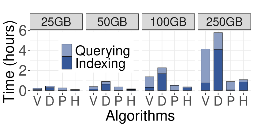
(a) Idx + 100 Queries

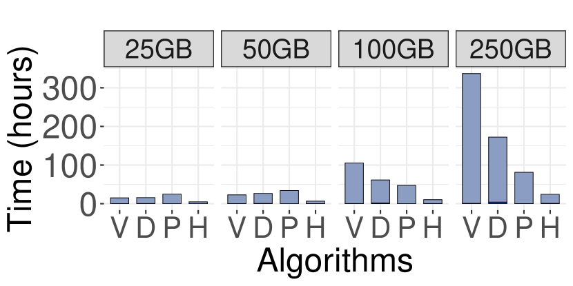
(b) Idx + 10K Queries

Figure 6. Scalability with increasing dataset sizes (100 1NN exact queries)

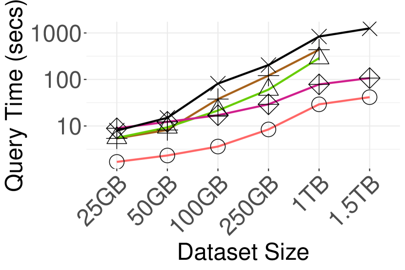
Figure 7. Scalability with dataset size

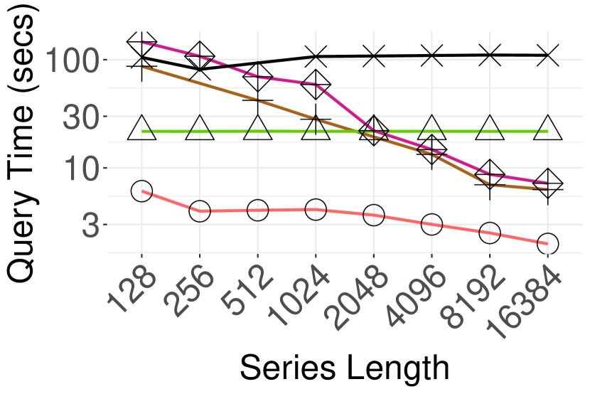
Figure 8. Scalability with series length

Scalability with Increasing Series Length. In this experiment, we study the performance of the algorithms as we vary the data series length. Figure 8 shows that Hercules (bottom curve) consistently performs 5-10x faster than the best other competitor, i.e., DSTree* for series of length 128-1024, and VA+file (followed very closely by Paris+) for series of length 2048-16384. Hercules outperforms PSCAN by at least one order of magnitude on all lengths.

Scalability with Increasing Query Difficulty. We now evaluate the performance of Hercules in terms of index construction time, and query answering on 100 and 10K exact 1NN queries of varying difficulty over the real datasets. Figure 9 shows the superiority of Hercules against its competitors for all datasets and query workloads. Observe that Hercules is the only method that, across all experiments, builds an index and answers 100/10K exact queries before the sequential scan (red dotted line) finishes execution.

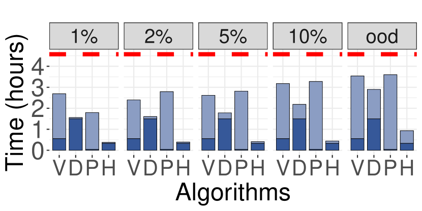
(a) Sald (100 Queries)

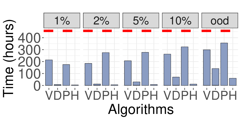
(b) Sald (10K Queries)

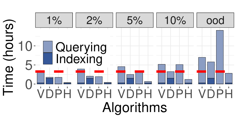
(c) Seismic (100 Queries)

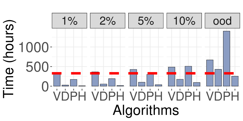
(d) Seismic (10K Queries)

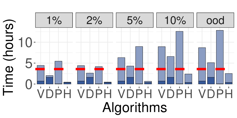
(e) Deep (100 Queries)

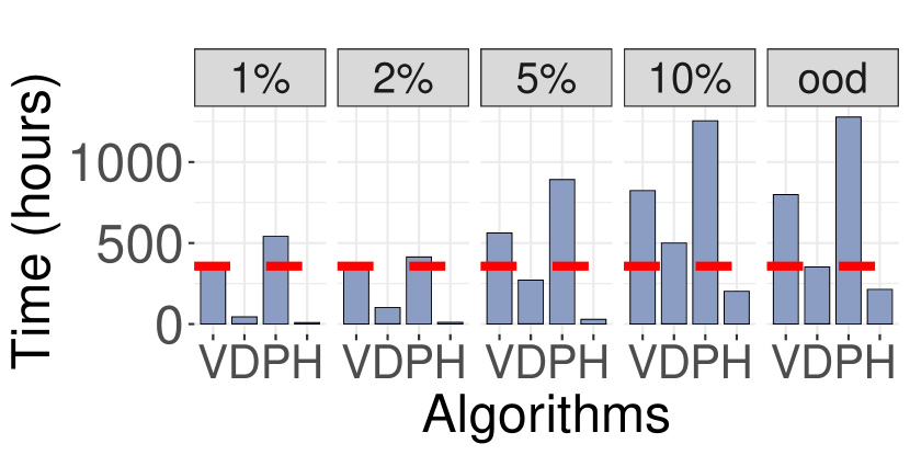
(f) Deep (10K Queries)

Figure 9. Scalability with query difficulty (combined indexing and query answering times)

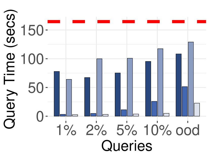
(a) Time (SALD)

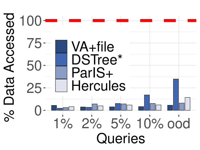
(b) Data (SALD)

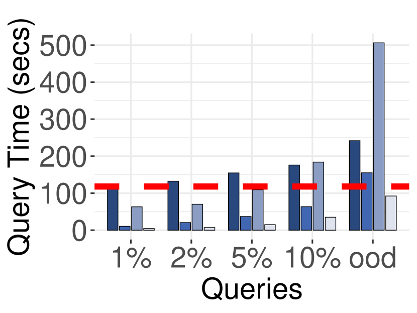
(c) Time (Seismic)

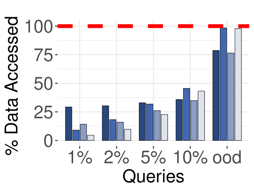
(d) Data (Seismic)

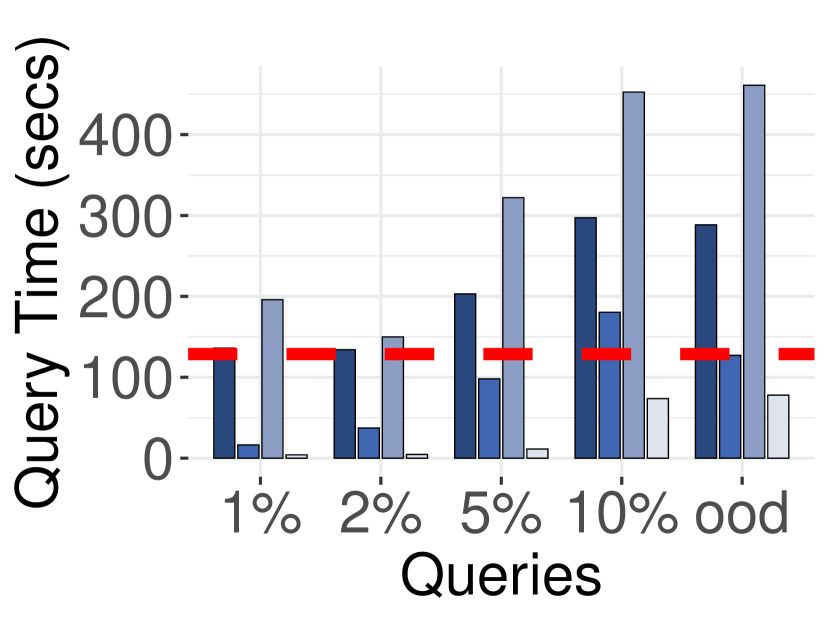
(e) Time (Deep)

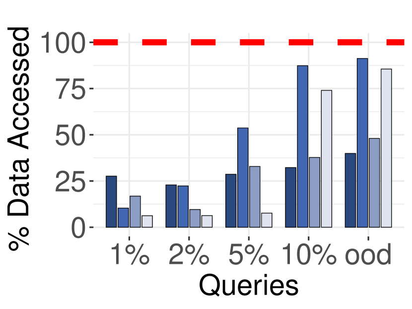
(f) Data (Deep)

Figure 10. Scalability with query difficulty (average query answering time and data accessed)

In Figure 10, we focus on the query answering performance for 1NN exact queries of varying difficulty. We report the query time and the percentage of data accessed, averaged per query. We observe that Hercules is superior to its competitors across the board. On the SALD dataset, Hercules is more than 2x faster than DSTree* on all queries, and 50x faster than ParIS+ on the easy (1%, 2%) to medium-hard queries (5%). Hercules maintains its good performance on the hard dataset $ood$, where it is 6x faster than ParIS+ despite the fact that it accesses double the amount of data on disk. We observe the same trend on the Seismic dataset: Hercules is the only index performing better than a sequential scan on the hard $ood$ dataset although it accesses 96% of the data. This is achieved thanks to two key design choices: the pruning thresholds based on which Hercules can choose to use a single thread to perform a skip-sequential scan (rather than using multiple threads to perform a large number of random I/O operations), and the LRDFile storage layout that leads to sequential disk I/O. The Deep dataset is notoriously hard (url, 2019a; Ge et al., 2014; Echihabi et al., 2018; Li et al., 2019), and we observe that indexes, except Hercules, start degenerating even on the easy queries (Figure 10(e)).

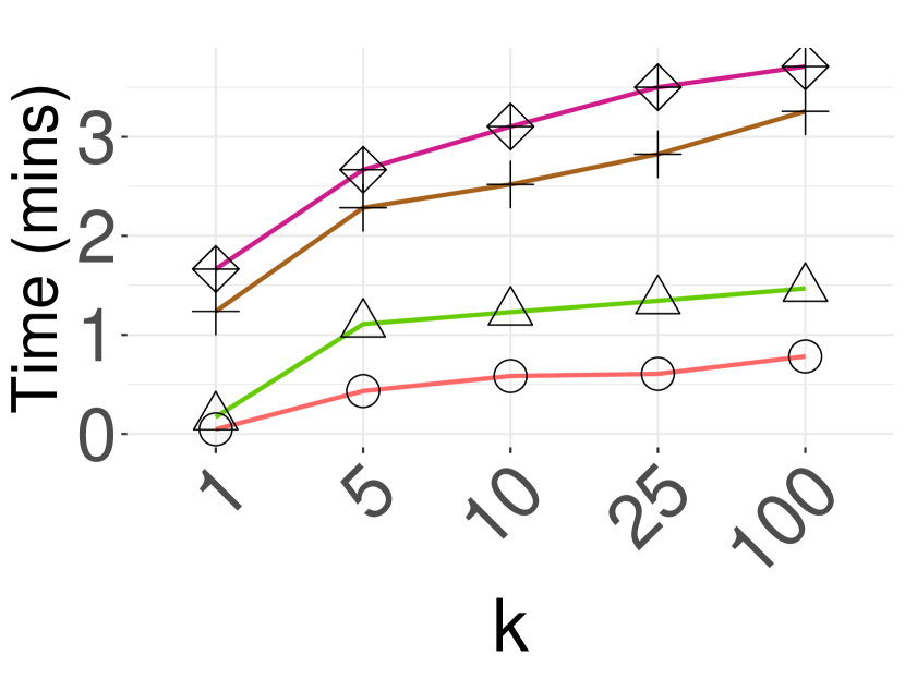
(a) Time (SALD)

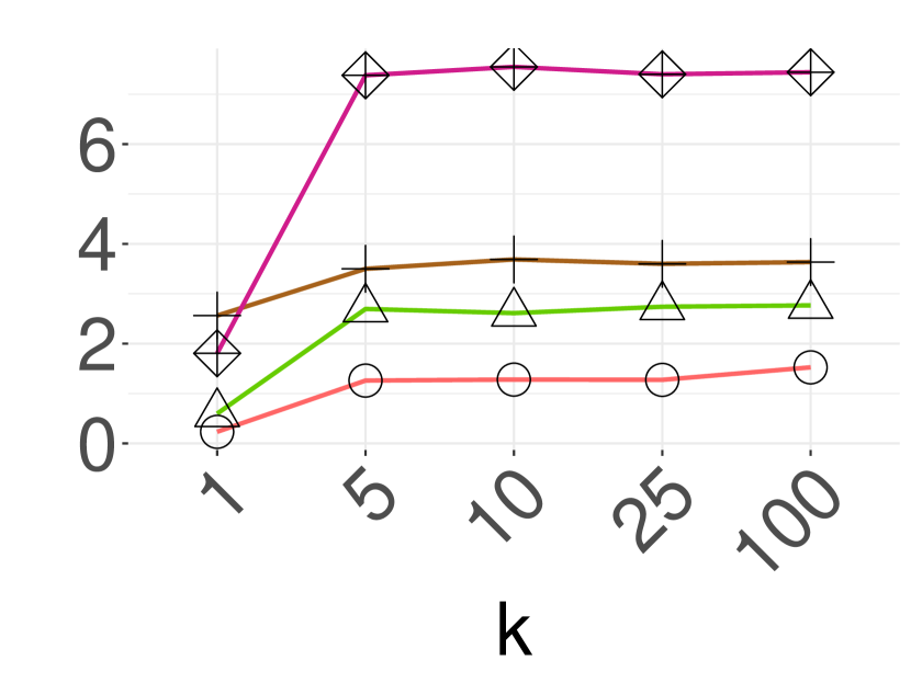
(b) Time (Seis.)

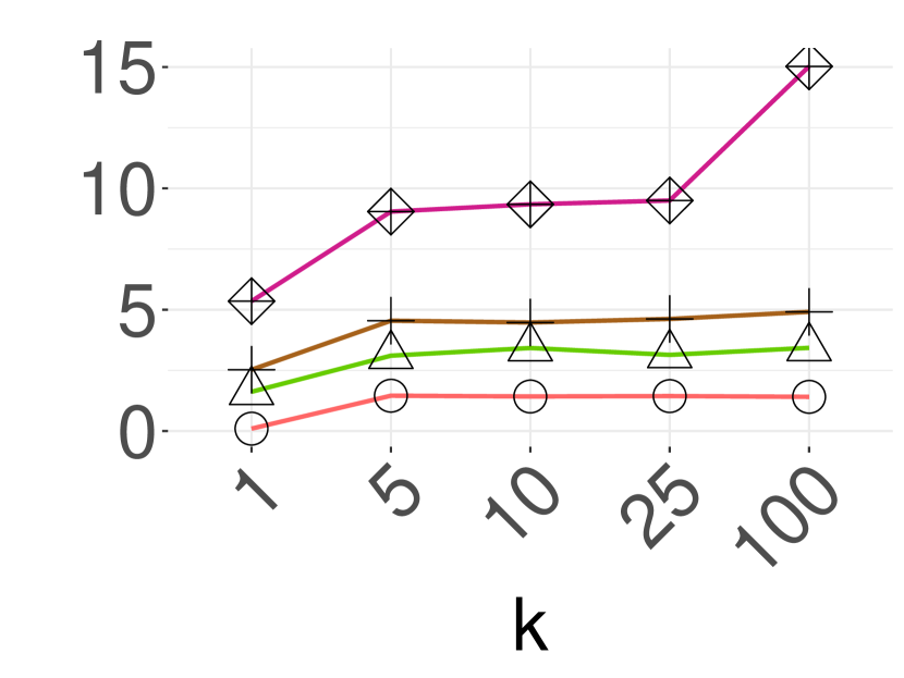
(c) Time (Deep)

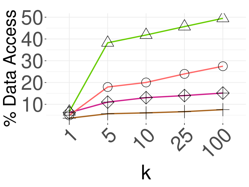
(d) Data (SALD)

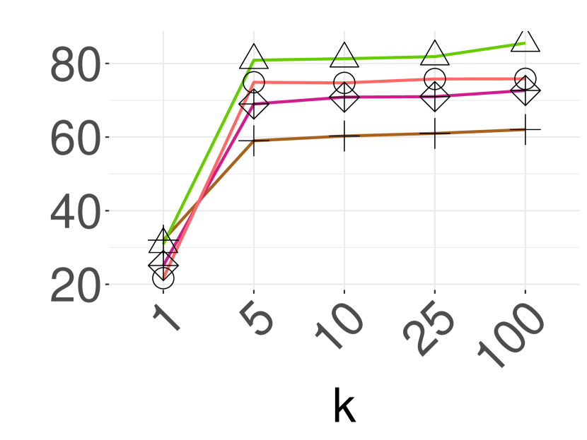
(e) Data (Seis.)

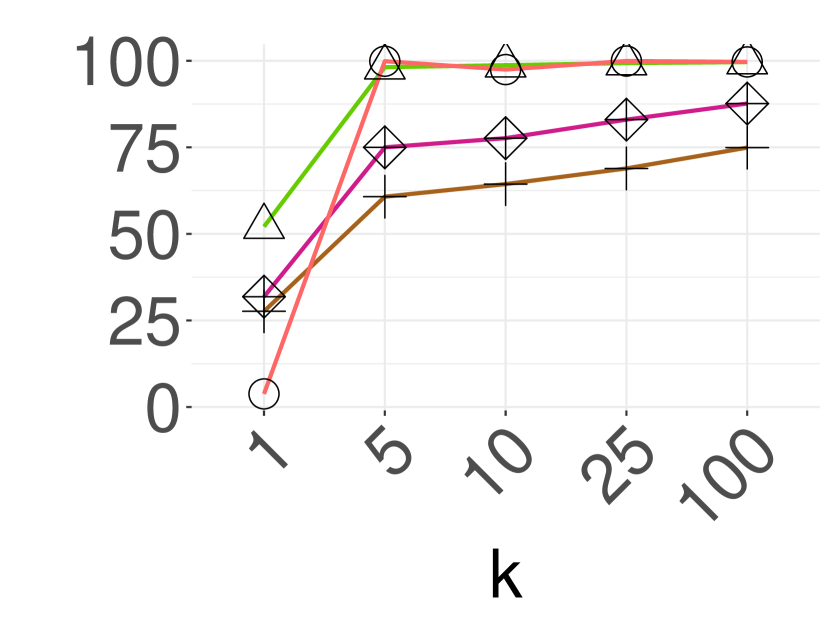
(f) Data (Deep)

Figure 11. Scalability with increasing k

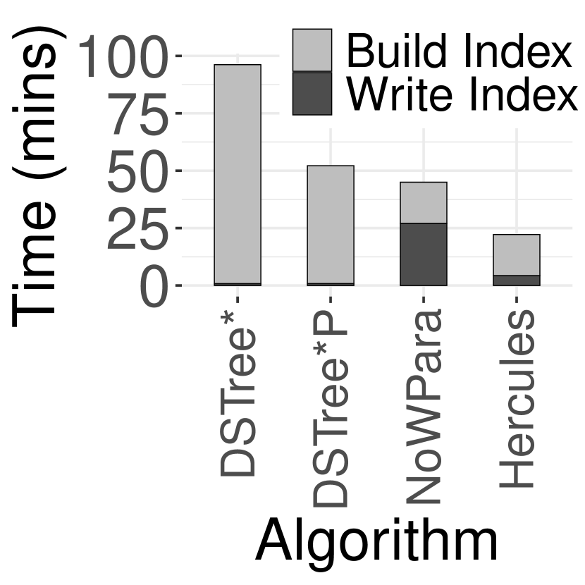
(a) Indexing

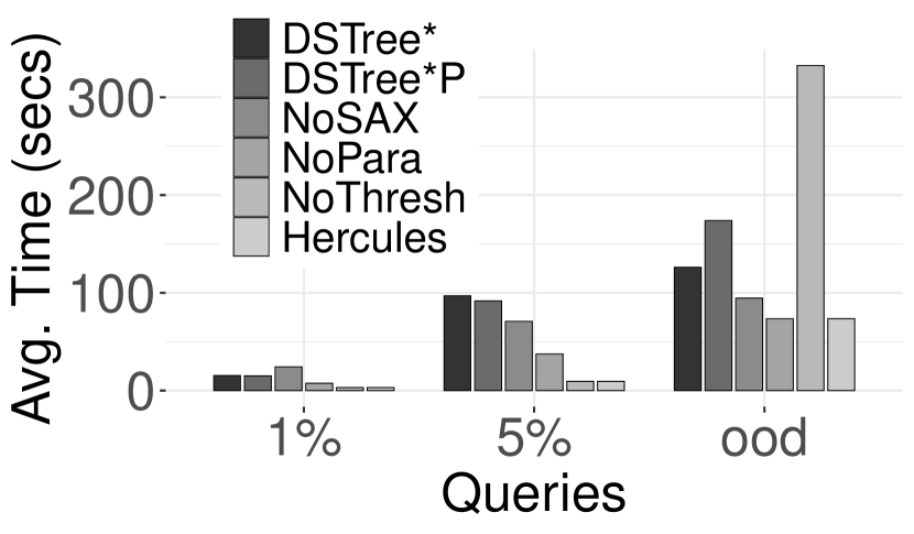
(b) Query Answering

Figure 12. Ablation Study

Overall, Hercules performs query answering 5.5x-63x faster than ParIS+, and 1.5x-10x faster than DSTree*. Once again, Hercules is the only index that wins across the board, performing 1.3x-9.4x faster than the second-best approach.

Scalability with Increasing k. In this scenario, we choose the medium-hard query workload $5\%$ for synthetic and real datasets of size 100GB, and vary the number of neighbors k in the kNN exact query workloads. We then measure the query time and percent of data accessed, averaged over all queries. Figure 11 shows that Hercules wins across the board for all values of $k$. Note that finding the first neighbor is the most costly operation for DSTree* and Hercules, while the performance of ParIS+ deteriorates as the number of neighbors increases. This is due to ParIS+ employing a skip-sequential query answering algorithm, with the raw data of the neighbors of a query being located anywhere in the dataset file, whereas in DSTree* and Hercules these data reside within the same subtree. (Note also that the skip-sequential algorithm used by Hercules operates on the LRDFile, which stores contiguously the data of each leaf.)

Ablation Study. In this experiment, we study the individual (not cumulative) effect on performance when removing each of the main building blocks of Hercules. Figure 12 summarizes the results on the Deep dataset (the other datasets and query workloads show similar trends (url, 2022)). Figure 12(a) shows the total index building and writing times for DSTree*, our parallelization of DSTree* (DSTree*P), Hercules without parallelization of index writing (NoWPara), and Hercules. Note that although DSTree*P exploits parallelism, it still incurs a very large index building cost. This is because insert workers need to lock entire paths (from the root to a leaf) for updating node statistics, causing a large synchronization overhead. In NoWPara, threads only lock leaf nodes since statistics of internal nodes are updated at the index writing phase, leading to a faster index building phase. However, the index writing phase is slower because of the additional calculations. By parallelizing index writing bottom-up, Hercules avoids some of the synchronization overhead, and achieves a much better performance.

We evaluate query answering in Figure 12(b), on three workloads of varying difficulty. We first remove the iSAX summarization and rely only on EAPCA for pruning (NoSAX), then we remove parallelization altogether from Hercules (NoPara), then we evaluate Hercules without the pruning thresholds (NoThresh), i.e., Hercules applies the same parallelization strategy to each query regardless of its difficulty. We observe that using only EAPCA pruning (NoSAX) always worsens performance, regardless of the query difficulty. Besides, the parallelization strategy used by Hercules is effective as it improves query efficiency (better than NoPara) for easy and medium-hard queries and has no negative effect on hard queries. Finally, we observe that the pruning thresholds contribute significantly to the efficiency of Hercules (better than NoThresh) on hard workloads (i.e., ood), and have no negative effect on the rest.

5. Conclusions and Future Work

We proposed Hercules, a novel index for exact similarity search over large data series collections. We demonstrated the superiority of Hercules against the state-of-the-art using an extensive experimental evaluation: Hercules performs between 1.3x-9.4x faster than the best competitor (which is different for the various datasets and workloads), and is the first index that achieves better performance than the optimized serial-scan algorithm across all workloads. In our future work, we will study in detail the behavior of Hercules in approximate query answering (with/without deterministic/probabilistic quality guarantees (Echihabi et al., 2019)).

- (1)
- url (2018) 2018. Lernaean Hydra Archive. http://www.mi.parisdescartes.fr/~themisp/dsseval/.
- url (2019a) 2019a. Faiss. https://github.com/facebookresearch/faiss/.
- url (2019b) 2019b. Return of Lernaean Hydra Archive. http://www.mi.parisdescartes.fr/~themisp/dsseval2/.
- url (2022) 2022. Hercules Archive. http://www.mi.parisdescartes.fr/~themisp/hercules/.
- Bach-Andersen et al. (2017) Martin Bach-Andersen, Bo Romer-Odgaard, and Ole Winther. 2017. Flexible Non-Linear Predictive Models for Large-Scale Wind Turbine Diagnostics. Wind Energy 20, 5 (2017), 753–764.
- Bagnall et al. (2019) Anthony J. Bagnall, Richard L. Cole, Themis Palpanas, and Konstantinos Zoumpatianos. 2019. Data Series Management (Dagstuhl Seminar 19282). Dagstuhl Reports 9, 7 (2019), 24–39. https://doi.org/10.4230/DagRep.9.7.24
- Beckmann et al. (1990) Norbert Beckmann, Hans-Peter Kriegel, Ralf Schneider, and Bernhard Seeger. 1990. The R*-tree: an efficient and robust access method for points and rectangles. In SIGMOD. 322–331.
- Boniol et al. (2022) Paul Boniol, Mohammed Meftah, Emmanuel Remy, and Themis Palpanas. 2022. dCAM: Dimension-wise Activation Map for Explaining Multivariate Data Series Classification. In SIGMOD.
- Camerra et al. (2010) Alessandro Camerra, Themis Palpanas, Jin Shieh, and Eamonn J. Keogh. 2010. iSAX 2.0: Indexing and Mining One Billion Time Series. In ICDM 2010, The 10th IEEE International Conference on Data Mining. 58–67.
- Camerra et al. (2014) Alessandro Camerra, Jin Shieh, Themis Palpanas, Thanawin Rakthanmanon, and Eamonn Keogh. 2014. Beyond One Billion Time Series: Indexing and Mining Very Large Time Series Collections with iSAX2+. KAIS 39, 1 (2014).
- Chakrabarti et al. (2002) Kaushik Chakrabarti, Eamonn Keogh, Sharad Mehrotra, and Michael Pazzani. 2002. Locally Adaptive Dimensionality Reduction for Indexing Large Time Series Databases. ACM Trans. Database Syst. 27, 2 (June 2002), 188–228. https://doi.org/10.1145/568518.568520
- Chatzigeorgakidis et al. (2021) Georgios Chatzigeorgakidis, Dimitrios Skoutas, Kostas Patroumpas, Themis Palpanas, Spiros Athanasiou, and Spiros Skiadopoulos. 2021. Twin Subsequence Search in Time Series. In Proceedings of the 24th International Conference on Extending Database Technology, EDBT 2021, Nicosia, Cyprus, March 23 - 26, 2021. 475–480.
- Chatzigeorgakidis et al. (2022) Georgios Chatzigeorgakidis, Dimitrios Skoutas, Kostas Patroumpas, Themis Palpanas, Spiros Athanasiou, and Spiros Skiadopoulos. 2022. Efficient Range and kNN Twin Subsequence Search in Time Series. TKDE (2022).
- Ciaccia et al. (1997) Paolo Ciaccia, Marco Patella, and Pavel Zezula. 1997. M-tree: An Efficient Access Method for Similarity Search in Metric Spaces. In Proceedings of the 23rd International Conference on Very Large Data Bases (VLDB’97), Matthias Jarke, Michael Carey, Klaus R. Dittrich, Fred Lochovsky, Pericles Loucopoulos, and Manfred A. Jeusfeld (Eds.). Morgan Kaufmann Publishers, Inc., Athens, Greece, 426–435.
- Echihabi (2020) Karima Echihabi. 2020. High-Dimensional Similarity Search: From Time Series to Deep Network Embeddings. In Proceedings of the 2020 International Conference on Management of Data, SIGMOD Conference 2020, Portland, OR, USA, June 14-19, 2020.
- Echihabi et al. (2020a) Karima Echihabi, Kostas Zoumpatianos, and Themis Palpanas. 2020a. Big Sequence Management: on Scalability (tutorial). In IEEE BigData.
- Echihabi et al. (2020b) Karima Echihabi, Kostas Zoumpatianos, and Themis Palpanas. 2020b. Scalable Machine Learning on High-Dimensional Vectors: From Data Series to Deep Network Embeddings. In WIMS.
- Echihabi et al. (2021a) Karima Echihabi, Kostas Zoumpatianos, and Themis Palpanas. 2021a. Big Sequence Management: Scaling Up and Out (tutorial). In EDBT.
- Echihabi et al. (2021b) Karima Echihabi, Kostas Zoumpatianos, and Themis Palpanas. 2021b. High-Dimensional Similarity Search for Scalable Data Science (tutorial). In ICDE.
- Echihabi et al. (2021c) Karima Echihabi, Kostas Zoumpatianos, and Themis Palpanas. 2021c. New Trends in High-D Vector Similarity Search: AI-driven, Progressive, and Distributed (tutorial). In VLDB.
- Echihabi et al. (2018) Karima Echihabi, Kostas Zoumpatianos, Themis Palpanas, and Houda Benbrahim. 2018. The Lernaean Hydra of Data Series Similarity Search: An Experimental Evaluation of the State of the Art. PVLDB 12, 2 (2018), 112–127.
- Echihabi et al. (2019) Karima Echihabi, Kostas Zoumpatianos, Themis Palpanas, and Houda Benbrahim. 2019. Return of the Lernaean Hydra: Experimental Evaluation of Data Series Approximate Similarity Search. PVLDB 13, 3 (2019), 402–419.
- Faloutsos et al. (1994) Christos Faloutsos, M. Ranganathan, and Yannis Manolopoulos. 1994. Fast Subsequence Matching in Time-Series Databases. In Proceedings of the 1994 ACM SIGMOD International Conference on Management of Data, Minneapolis, Minnesota, USA, May 24-27, 1994. 419–429.
- Ferhatosmanoglu et al. (2000) Hakan Ferhatosmanoglu, Ertem Tuncel, Divyakant Agrawal, and Amr El Abbadi. 2000. Vector Approximation Based Indexing for Non-uniform High Dimensional Data Sets. In Proceedings of the Ninth International Conference on Information and Knowledge Management (McLean, Virginia, USA) (CIKM ’00). ACM, New York, NY, USA, 202–209. https://doi.org/10.1145/354756.354820
- for Seismology with Artificial Intelligence (2018) Incorporated Research Institutions for Seismology with Artificial Intelligence. 2018. Seismic Data Access. http://ds.iris.edu/data/access/.
- Ge et al. (2014) Tiezheng Ge, Kaiming He, Qifa Ke, and Jian Sun. 2014. Optimized Product Quantization. IEEE Trans. Pattern Anal. Mach. Intell. 36, 4 (April 2014), 744–755. https://doi.org/10.1109/TPAMI.2013.240
- Gogolou et al. (2020) Anna Gogolou, Theophanis Tsandilas, Karima Echihabi, Anastasia Bezerianos, and Themis Palpanas. 2020. Data Series Progressive Similarity Search with Probabilistic Quality Guarantees. In SIGMOD.
- Gogolou et al. (2019) Anna Gogolou, Theophanis Tsandilas, Themis Palpanas, and Anastasia Bezerianos. 2019. Progressive Similarity Search on Time Series Data. In Proceedings of the Workshops of the EDBT/ICDT 2019 Joint Conference.
- Kashino et al. (1999) Kunio Kashino, Gavin Smith, and Hiroshi Murase. 1999. Time-series active search for quick retrieval of audio and video. In ICASSP.
- Keogh et al. (2001) Eamonn Keogh, Kaushik Chakrabarti, Michael Pazzani, and Sharad Mehrotra. 2001. Dimensionality Reduction for Fast Similarity Search in Large Time Series Databases. Knowledge and Information Systems 3, 3 (2001), 263–286. https://doi.org/10.1007/PL00011669
- Keogh and Ratanamahatana (2005) Eamonn Keogh and Chotirat Ann Ratanamahatana. 2005. Exact Indexing of Dynamic Time Warping. Knowl. Inf. Syst. 7, 3 (March 2005), 358–386. https://doi.org/10.1007/s10115-004-0154-9
- Knieling et al. (2017) S. Knieling, J. Niediek, E. Kutter, J. Bostroem, C.E. Elger, and F. Mormann. 2017. An online adaptive screening procedure for selective neuronal responses. Journal of Neuroscience Methods 291, Supplement C (2017), 36 – 42. https://doi.org/10.1016/j.jneumeth.2017.08.002
- Kondylakis et al. (2019) Haridimos Kondylakis, Niv Dayan, Kostas Zoumpatianos, and Themis Palpanas. 2019. Coconut: sortable summarizations for scalable indexes over static and streaming data series. VLDBJ (2019).
- Laviron et al. (2021) Pauline Laviron, Xueqi Dai, Bérénice Huquet, and Themis Palpanas. 2021. Electricity Demand Activation Extraction: From Known to Unknown Signatures, Using Similarity Search. In e-Energy ’21: The Twelfth ACM International Conference on Future Energy Systems. 148–159.
- Levchenko et al. (2021) Oleksandra Levchenko, Boyan Kolev, Djamel Edine Yagoubi, Reza Akbarinia, Florent Masseglia, Themis Palpanas, Dennis E. Shasha, and Patrick Valduriez. 2021. BestNeighbor: efficient evaluation of kNN queries on large time series databases. Knowl. Inf. Syst. 63, 2 (2021), 349–378.
- Li et al. (2019) W. Li, Y. Zhang, Y. Sun, W. Wang, M. Li, W. Zhang, and X. Lin. 2019. Approximate Nearest Neighbor Search on High Dimensional Data - Experiments, Analyses, and Improvement. IEEE Transactions on Knowledge and Data Engineering (2019), 1–1. https://doi.org/10.1109/TKDE.2019.2909204
- Lin et al. (2003) Jessica Lin, Eamonn J. Keogh, Stefano Lonardi, and Bill Yuan-chi Chiu. 2003. A symbolic representation of time series, with implications for streaming algorithms. In Proceedings of the 8th ACM SIGMOD workshop on Research issues in data mining and knowledge discovery, DMKD 2003, San Diego, California, USA, June 13, 2003. 2–11. https://doi.org/10.1145/882082.882086
- Linardi and Palpanas (2018) Michele Linardi and Themis Palpanas. 2018. ULISSE: ULtra compact Index for Variable-Length Similarity SEarch in Data Series. In ICDE.
- Linardi et al. (2018) Michele Linardi, Yan Zhu, Themis Palpanas, and Eamonn J. Keogh. 2018. Matrix Profile X: VALMOD - Scalable Discovery of Variable-Length Motifs in Data Series. SIGMOD.
- Linardi et al. (2020) Michele Linardi, Yan Zhu, Themis Palpanas, and Eamonn J. Keogh. 2020. Matrix profile goes MAD: variable-length motif and discord discovery in data series. Data Min. Knowl. Discov. 34, 4 (2020), 1022–1071. https://doi.org/10.1007/s10618-020-00685-w
- Maccone (2007) Claudio Maccone. 2007. Advantages of Karhunen–Loève transform over fast Fourier transform for planetary radar and space debris detection. Acta Astronautica 60, 8 (2007), 775 – 779. https://doi.org/10.1016/j.actaastro.2006.08.015
- Mirylenka et al. (2016) Katsiaryna Mirylenka, Vassilis Christophides, Themis Palpanas, Ioannis Pefkianakis, and Martin May. 2016. Characterizing Home Device Usage From Wireless Traffic Time Series. In EDBT. 551–562. https://doi.org/10.5441/002/edbt.2016.51
- Palpanas (2015) Themis Palpanas. 2015. Data Series Management: The Road to Big Sequence Analytics. SIGMOD Record (2015).
- Palpanas (2016) Themis Palpanas. 2016. Big Sequence Management: A glimpse of the Past, the Present, and the Future.. In SOFSEM (Lecture Notes in Computer Science), Rusins Martins Freivalds, Gregor Engels, and Barbara Catania (Eds.), Vol. 9587. Springer, 63–80. http://dblp.uni-trier.de/db/conf/sofsem/sofsem2016.html#Palpanas16
- Palpanas (2020) Themis Palpanas. 2020. Evolution of a Data Series Index - The iSAX Family of Data Series Indexes. CCIS 1197 (2020).
- Palpanas and Beckmann (2019) Themis Palpanas and Volker Beckmann. 2019. Report on the First and Second Interdisciplinary Time Series Analysis Workshop (ITISA). SIGMOD Rec. 48, 3 (2019).
- Paparrizos et al. (2022) John Paparrizos, Yuhao Kang, Paul Boniol, Ruey S. Tsay, Themis Palpanas, and Michael J. Franklin. 2022. TSB-UAD: An End-to-End Benchmark Suite for Univariate Time-Series Anomaly Detection. PVLDB (2022).
- Paraskevopoulos et al. (2013) Pavlos Paraskevopoulos, Thanh-Cong Dinh, Zolzaya Dashdorj, Themis Palpanas, and Luciano Serafini. 2013. Identification and Characterization of Human Behavior Patterns from Mobile Phone Data. In D4D Challenge session, NetMob.
- Peng et al. (2018) Botao Peng, Panagiota Fatourou, and Themis Palpanas. 2018. ParIS: The Next Destination for Fast Data Series Indexing and Query Answering. IEEE BigData (2018).
- Peng et al. (2020) Botao Peng, Panagiota Fatourou, and Themis Palpanas. 2020. MESSI: In-Memory Data Series Indexing. ICDE (2020).
- Peng et al. (2021a) Botao Peng, Panagiota Fatourou, and Themis Palpanas. 2021a. Fast Data Series Indexing for In-Memory Data. VLDBJ 30, 6 (2021).
- Peng et al. (2021b) Botao Peng, Panagiota Fatourou, and Themis Palpanas. 2021b. SING: Sequence Indexing Using GPUs. In Proceedings of the International Conference on Data Engineering (ICDE).
- Peng et al. (2021c) Botao Peng, Themis Palpanas, and Panagiota Fatourou. 2021c. ParIS+: Data Series Indexing on Multi-core Architectures. TKDE 33(5) (2021).
- Rakthanmanon et al. (2012) Thanawin Rakthanmanon, Bilson J. L. Campana, Abdullah Mueen, Gustavo E. A. P. A. Batista, M. Brandon Westover, Qiang Zhu, Jesin Zakaria, and Eamonn J. Keogh. 2012. Searching and mining trillions of time series subsequences under dynamic time warping.. In KDD.
- Raza et al. (2015) Usman Raza, Alessandro Camerra, Amy L. Murphy, Themis Palpanas, and Gian Pietro Picco. 2015. Practical Data Prediction for Real-World Wireless Sensor Networks. IEEE Trans. Knowl. Data Eng. 27, 8 (2015).
- Schäfer and Högqvist (2012) Patrick Schäfer and Mikael Högqvist. 2012. SFA: A Symbolic Fourier Approximation and Index for Similarity Search in High Dimensional Datasets. In Proceedings of the 15th International Conference on Extending Database Technology (Berlin, Germany) (EDBT ’12). ACM, New York, NY, USA, 516–527. https://doi.org/10.1145/2247596.2247656
- Shasha (1999) Dennis Shasha. 1999. Tuning Time Series Queries in Finance: Case Studies and Recommendations. IEEE Data Eng. Bull. 22, 2 (1999), 40–46.
- Shieh and Keogh (2008) Jin Shieh and Eamonn Keogh. 2008. iSAX: Indexing and Mining Terabyte Sized Time Series. In Proceedings of the 14th ACM SIGKDD International Conference on Knowledge Discovery and Data Mining (Las Vegas, Nevada, USA) (KDD ’08). ACM, New York, NY, USA, 623–631. https://doi.org/10.1145/1401890.1401966
- Shieh and Keogh (2009) Jin Shieh and Eamonn Keogh. 2009. iSAX: disk-aware mining and indexing of massive time series datasets. DMKD (2009).
- Skoltech Computer Vision (2018) Skoltech Computer Vision. 2018. Deep billion-scale indexing.
- Soldi et al. (2014) S Soldi, Volker Beckmann, WH Baumgartner, Gabriele Ponti, Chris R Shrader, P Lubiński, HA Krimm, F Mattana, and Jack Tueller. 2014. Long-term variability of AGN at hard X-rays. Astronomy & Astrophysics 563 (2014), A57.
- University (2018) Southwest University. 2018. Southwest University Adult Lifespan Dataset (SALD). http://fcon_1000.projects.nitrc.org/indi/retro/sald.html?utm_source=newsletter&utm_medium=email&utm_content=See%20Data&utm_campaign=indi-1
- Wang and Palpanas (2021) Qitong Wang and Themis Palpanas. 2021. Deep Learning Embeddings for Data Series Similarity Search. In SIGKDD.
- Wang et al. (2013) Yang Wang, Peng Wang, Jian Pei, Wei Wang, and Sheng Huang. 2013. A Data-adaptive and Dynamic Segmentation Index for Whole Matching on Time Series. PVLDB 6, 10 (2013), 793–804. http://dblp.uni-trier.de/db/journals/pvldb/pvldb6.html#WangWPWH13
- Yagoubi et al. (2017) Djamel Edine Yagoubi, Reza Akbarinia, Florent Masseglia, and Themis Palpanas. 2017. DPiSAX: Massively Distributed Partitioned iSAX. In 2017 IEEE International Conference on Data Mining, ICDM 2017, New Orleans, LA, USA, November 18-21, 2017. 1135–1140.
- Yagoubi et al. (2020) Djamel-Edine Yagoubi, Reza Akbarinia, Florent Masseglia, and Themis Palpanas. 2020. Massively Distributed Time Series Indexing and Querying. TKDE 31(1) (2020).
- Zhang et al. (2019) L. Zhang, N. Alghamdi, M. Y. Eltabakh, and E. A. Rundensteiner. 2019. TARDIS: Distributed Indexing Framework for Big Time Series Data. In 2019 IEEE 35th International Conference on Data Engineering (ICDE). 1202–1213. https://doi.org/10.1109/ICDE.2019.00110
- Zoumpatianos et al. (2016) Kostas Zoumpatianos, Stratos Idreos, and Themis Palpanas. 2016. ADS: the adaptive data series index. The VLDB Journal 25, 6 (2016), 843–866. https://doi.org/10.1007/s00778-016-0442-5
- Zoumpatianos et al. (2018) Kostas Zoumpatianos, Yin Lou, Ioana Ileana, Themis Palpanas, and Johannes Gehrke. 2018. Generating Data Series Query Workloads. The VLDB Journal 27, 6 (Dec. 2018), 823–846. https://doi.org/10.1007/s00778-018-0513-x
- Zoumpatianos et al. (2015) Kostas Zoumpatianos, Yin Lou, Themis Palpanas, and Johannes Gehrke. 2015. Query Workloads for Data Series Indexes. In KDD.
- Zoumpatianos and Palpanas (2018) Kostas Zoumpatianos and Themis Palpanas. 2018. Data Series Management: Fulfilling the Need for Big Sequence Analytics. In ICDE.