On integrability of the deformed Ruijsenaars-Schneider system

We find integrals of motion for the recently introduced deformed Ruijsenaars-Schneider many-body system which is the dynamical system for poles of elliptic solutions to the Toda lattice with constraint of type B. Our method is based on the fact that equations of motion for this system coincide with those for pairs of Ruijsenaars-Schneider particles which stick together preserving a special fixed distance between the particles.

1 Introduction

Integrable many-body systems of classical mechanics play a significant role in modern mathematical physics. They are interesting and meaningful from both mathematical and physical points of view and have important applications and deep connections with different problems in mathematics and physics. The history of integrable many-body systems starts from the famous Calogero-Moser (CM) model [2]-[5] which exists in rational, trigonometric or hyperbolic and elliptic versions. In the most general elliptic case the equations of motion for the $N$-body CM system are

$$\ddot{x}_{i}=4\sum_{j\neq i}^{N}\wp^{\prime}(x_{ij}),\qquad x_{ij}=x_{i}-x_{j},$$ (1.1)

where dot means the time derivative. Throughout the paper, we use the standard Weierstrass $\sigma$-, $\zeta$- and $\wp$-functions $\sigma(x)$, $\zeta(x)=\sigma^{\prime}(x)/\sigma(x)$ and $\wp(x)=-\zeta^{\prime}(x)$ (see Appendix A for their definition and properties). Degenerating the elliptic functions to trigonometric and rational ones, one obtains the trigonometric and rational versions of the CM model. The elliptic CM model is Hamiltonian and completely integrable, i.e., it has $N$ independent integrals of motion in involution. Integrability of the model was proved by different methods in [6] and [7], see also the book [8].

Later it was discovered [9, 10] that there exists a one-parametric deformation of the CM system preserving integrability, often referred to as relativistic extension. The parameter of the deformation, $\eta$, in this interpretation is the inverse velocity of light. This model is now called the Ruijsenaars-Schneider (RS) system. Again, in its most general version the interaction between particles is described by elliptic functions. The equations of motion are

$$\ddot{x}_{i}+\sum_{j\neq i}^{N}\dot{x}_{i}\dot{x}_{j}\Bigl{(}\zeta(x_{ij}+\eta)+\zeta(x_{ij}-\eta)-2\zeta(x_{ij})\Bigr{)}=0.$$ (1.2)

A properly taken limit $\eta\to 0$ leads to equations (1.1). The RS system is Hamiltonian with the Hamiltonian

$${\sf H}_{1}=\sum_{i=1}^{N}e^{p_{i}}\prod_{j\neq i}^{N}\frac{\sigma(x_{ij}+\eta)}{\sigma(x_{ij})}.$$ (1.3)

Integrability of the RS system was proved in [10]. It has conserved quantities ${\sf H}_{k}$, $\bar{\sf H}_{k}$ $k\in\mbox{\Bbb N}$, which are higher Hamiltonians in involution (for the $N$-particle system the first $N$ of them are independent).

Since the seminal works [11]-[14] it became a common knowledge that the integrable many-body systems of Calogero-Moser type describe dynamics of poles of singular solutions (in general, elliptic solutions) to nonlinear integrable differential equations such as Korteveg-de Vries (KdV) and Kadomtsev-Petviashvili (KP) equations. In [15] it was shown that the RS system plays the same role for singular solutions to the Toda lattice equation which can be thought of as an integrable difference deformation of the KP equation. (On the Toda lattice side, the parameter $\eta$ can be identified with the lattice spacing.) Namely, the time evolution of poles in the time $t=t_{1}$ of the Toda hierarchy coincides with the RS dynamics according to the equations of motion (1.2). Later this correspondence was extended [16] to the level of hierarchies: the evolution of poles in the higher times $t_{k}$ and $\bar{t}_{k}$ of the Toda hierarchy was shown to be given by the RS Hamiltonian flows with the higher Hamiltonians ${\sf H}_{k}$ and $\bar{\sf H}_{k}$.

Recently, a deformation of the RS model was introduced [17] as a dynamical system describing time evolution of poles of elliptic solutions to the Toda lattice with the constraint of type B [18]. Equations of motion of the deformed RS system are

$$\ddot{x}_{i}+\sum_{j\neq i}^{N}\dot{x}_{i}\dot{x}_{j}\Bigl{(}\zeta(x_{ij}+\eta)+\zeta(x_{ij}-\eta)-2\zeta(x_{ij})\Bigr{)}+g(U_{i}^{-}-U_{i}^{+})=0,$$ (1.4)

where

$$U_{i}^{\pm}=\prod_{j\neq i}^{N}U^{\pm}(x_{ij}),\qquad U^{\pm}(x_{ij})=\frac{\sigma(x_{ij}\pm 2\eta)\sigma(x_{ij}\mp\eta)}{\sigma(x_{ij}\pm\eta)\sigma(x_{ij})}$$ (1.5)

and $g$ is the deformation parameter. At $g=0$ we have the RS system. It is evident that $g\neq 0$ can be eliminated from the formulas by re-scaling of the time variable $t\to g^{-1/2}t$. In what follows we fix $g$ to be $g=\sigma(2\eta)$ without loss of generality. With this choice of $g$, equations (1.4) are exactly the same as they appear as the dynamical equations for poles with the convention on the choice of the time variable adopted in the Toda lattice with the constraint of type B. In [17] it was shown that the $\eta\to 0$ limit of equations (1.4) reproduces the equations of motion

$$\ddot{x}_{i}+6\sum_{j\neq i}^{N}(\dot{x}_{i}+\dot{x}_{j})\wp^{\prime}(x_{ij})-72\sum_{j,k\neq i,j\neq k}\wp(x_{ij})\wp^{\prime}(x_{ik})=0$$ (1.6)

obtained in [19] for dynamics of poles of elliptic solutions to the B-version of the KP equation (BKP).

In [17] it was also shown that that the system (1.4) can be obtained by restriction of the Hamiltonian flow with the Hamiltonian ${\sf H}_{1}^{-}={\sf H}_{1}-\bar{\sf H}_{1}$ of the $N=2N_{0}$-particle RS system to the half-dimensional subspace ${\cal P}\subset{\cal F}$ of the $4N_{0}$-dimensional phase space ${\cal F}$ corresponding to the configurations in which the $2N_{0}$ particles stick together joining in $N_{0}$ pairs such that the distance between particles in each pair is equal to $\eta$. Such configurations are immediately destroyed by the flow with the Hamiltonian ${\sf H}_{1}^{+}={\sf H}_{1}+\bar{\sf H}_{1}$ but are preserved by the flow with the Hamiltonian ${\sf H}_{1}^{-}={\sf H}_{1}-\bar{\sf H}_{1}$ and the corresponding dynamics can be restricted to the subspace ${\cal P}$. The restriction gives equations (1.4), where $N$ should be substituted by $N_{0}$, with $x_{i}$ ($i=1,\ldots,N_{0}$) being the coordinate of the $i$th pair moving as a whole thing with the fixed distance between the two particles.

In this paper we provide evidence of integrability of the deformed RS system (1.4). To wit, we obtain the complete set of independent integrals of motion in the explicit form. Our method is based on the fact (which is proved in the paper) that the subspace ${\cal P}$ is preserved not only by the flows with the Hamiltonian ${\sf H}_{1}^{-}$ but also by all higher Hamiltonian flows with the Hamiltonians ${\sf H}_{k}^{-}$. (However, the flows with the Hamiltonians ${\sf H}_{k}^{+}$ do not preserve the space ${\cal P}$.) This gives the possibility to obtain the integrals of motion of the $N_{0}$-particle deformed RS system by restriction of the known integrals of motion for the $2N_{0}$-particle RS system to the subspace ${\cal P}$ of pairs, and this is what we do in the present paper.

The main result of this paper is the following explicit expressions for integrals of motion of the system (1.4) (with $g=\sigma(2\eta)$):

$$\begin{array}[]{l}\displaystyle{J_{n}=\frac{1}{2}\sum_{m=0}^{[n/2]}\frac{\sigma(n\eta)\sigma^{2m-n}(\eta)}{m!\,(n\!-\!2m)!}\sum_{[i_{1}\ldots i_{n-m}]}^{N}\!\dot{x}_{i_{m+1}}\ldots\dot{x}_{i_{n-m}}\!\!\!\!\prod_{\alpha,\beta=m+1\atop\alpha<\beta}^{n-m}\!V(x_{i_{\alpha}i_{\beta}})}\\ \\ \displaystyle{\phantom{aaaaaaaaaaaaaaaa}\times\left[\prod_{\gamma=1}^{m}\prod_{\ell\neq i_{1},\ldots,i_{n-m}}^{N}\!\!\!\!U^{+}(x_{i_{\gamma}\ell})+\prod_{\gamma=1}^{m}\prod_{\ell\neq i_{1},\ldots,i_{n-m}}^{N}\!\!\!\!U^{-}(x_{i_{\gamma}\ell})\right],}\end{array}$$ (1.7)

where

$$V(x_{ij})=\frac{\sigma^{2}(x_{ij})}{\sigma(x_{ij}\!+\!\eta)\sigma(x_{ij}\!-\!\eta)}$$

and $U^{\pm}(x_{ij})$ is given in (1.5). In (1.7) $n=1,\ldots,N$ and $\displaystyle{\sum_{[i_{1}\ldots i_{n-m}]}^{N}}$ means summation over all distinct indexes $i_{1},\ldots,i_{n-m}$ from $1$ to $N$; $[n/2]$ is the integer part of $n/2$. At $m=0$, the product $\displaystyle{\prod_{\gamma=1}^{0}}$ in the second line of (1.7) should be put equal to $1$. Similarly, at $2m=n$ the product $\dot{x}_{i_{m+1}}\ldots\dot{x}_{i_{n-m}}$ should also be put equal to $1$. Here are some examples for small values of $n$:

$$\begin{array}[]{l}\displaystyle{J_{1}=\sum_{i=1}\dot{x}_{i},}\\ \\ \displaystyle{J_{2}=\frac{\sigma(2\eta)}{2\sigma^{2}(\eta)}\left[\sum_{i\neq j}\dot{x}_{i}\dot{x}_{j}V(x_{ij})+\sigma^{2}(\eta)\sum_{i}\Bigl{(}\prod_{\ell\neq i}U^{+}(x_{i\ell})+\prod_{\ell\neq i}U^{-}(x_{i\ell})\Bigr{)}\right],}\\ \\ \!\!\!\begin{array}[]{l}\displaystyle{J_{3}=\frac{\sigma(3\eta)}{6\sigma^{3}(\eta)}\left[\sum_{i\neq j,k,\,j\neq k}\dot{x}_{i}\dot{x}_{j}\dot{x}_{k}V(x_{ij})V(x_{ik})V(x_{jk})\right.}\\ \displaystyle{\phantom{aaaaaaaaaaaaaaaaaaaa}\left.+\,\,3\sigma^{2}(\eta)\sum_{i\neq j}\dot{x}_{j}\Bigl{(}\prod_{\ell\neq i,j}U^{+}(x_{i\ell})+\prod_{\ell\neq i,j}U^{-}(x_{i\ell})\Bigr{)}\right].}\end{array}\end{array}$$ (1.8)

Note that the $m=0$ term in (1.7) is the $n$th integral of motion of the RS system (1.2).

We also find the generating function of the integrals of motion:

$$R(z,\lambda)=\det_{1\leq i,j\leq N}\Bigl{(}z\delta_{ij}-\dot{x}_{i}\phi(x_{ij}\!-\!\eta,\lambda)-\sigma(2\eta)z^{-1}U_{i}^{-}\phi(x_{ij}\!-\!2\eta,\lambda)\Bigr{)},$$ (1.9)

where

$$\phi(x,\lambda):=\frac{\sigma(x+\lambda)}{\sigma(\lambda)\sigma(x)}.$$ (1.10)

The equation $R(z,\lambda)=0$ defines the spectral curve which is an integral of motion.

The organization of the paper is as follows. In Section 2 we remind the main facts about the elliptic RS model. In Section 3 we show, reproducing the result of [17], that the dynamics of the deformed RS system is the ${\sf H}_{1}^{-}$-flow of the RS system restricted to the space of pairs. The core of the paper is Section 4, where we prove that the space of pairs is invariant under all higher ${\sf H}^{-}_{k}$-flows and find integrals of motion of the deformed RS system in the explicit form. The generating function of the integrals of motion is found in Section 5. In Section 6 we make concluding remarks and list some open problems. There are also two appendices. In Appendix A the definition and main properties of the Weierstrass functions are presented. In Appendix B we prove an identity for elliptic functions which is the key identity for the proof of Theorem 4.1 in Section 4.

This paper has grown up from our joint works [17, 18] with Igor Krichever. Soon after the present work was started, my older friend and co-author Igor Krichever passed away. He worked till the last his days, and we had several illuminating conversations. With sorrow and gratefulness, I dedicate this paper to his memory.

2 The RS system

Here we collect the main facts on the elliptic RS system following the paper [10].

The $N$-particle elliptic RS system is a completely integrable model. The canonical Poisson brackets between coordinates and momenta are $\{x_{i},p_{j}\}=\delta_{ij}$. The integrals of motion in involution have the form

$${\sf I}_{n}=\sum_{{\cal I}\subset\{1,\ldots,N\},\,|{\cal I}|=n}\exp\Bigl{(}\sum_{i\in{\cal I}}p_{i}\Bigr{)}\prod_{i\in{\cal I},j\notin{\cal I}}\frac{\sigma(x_{ij}+\eta)}{\sigma(x_{ij})},\quad n=1,\ldots,N.$$ (2.1)

It is natural to put ${\sf I}_{0}=1$. Important particular cases of (2.1) are

$${\sf I}_{1}=\sum_{i=1}^{N}e^{p_{i}}\prod_{j\neq i}\frac{\sigma(x_{ij}+\eta)}{\sigma(x_{ij})}$$ (2.2)

which is the Hamiltonian ${\sf H}_{1}$ of the chiral RS model and

$${\sf I}_{N}=\exp\Bigl{(}\sum_{i=1}^{N}p_{i}\Bigr{)}.$$ (2.3)

Comparing to the paper [10], our formulas differ by the canonical transformation

$$e^{p_{i}}\to e^{p_{i}}\prod_{j\neq i}\frac{\sigma^{1/2}(x_{ij}+\eta)}{\sigma^{1/2}(x_{ij}-\eta)},\quad x_{i}\to x_{i},$$

which allows one to eliminate square roots in the formulas from [10].

Let us denote the time variable of the Hamiltonian flow with the Hamiltonian ${\sf H}_{1}=I_{1}$ by $t_{1}$. The velocities of the particles are

$$\stackrel{{\scriptstyle*}}{{x}}_{i}=\frac{\partial{\sf H}_{1}}{\partial p_{i}}=e^{p_{i}}\prod_{j\neq i}\frac{\sigma(x_{ij}+\eta)}{\sigma(x_{ij})},$$ (2.4)

where star means the $t_{1}$-derivative. Note that in terms of velocities the integrals of motion (2.1) read:

$${\sf I}_{n}=\frac{1}{n!}\sum_{[i_{1}\ldots i_{n}]}^{N}\!\!\stackrel{{\scriptstyle*}}{{x}}_{i_{1}}\ldots\stackrel{{\scriptstyle*}}{{x}}_{i_{n}}\!\!\!\prod_{\alpha,\beta=1\atop\alpha<\beta}^{n}\!\frac{\sigma^{2}(x_{i_{\alpha}i_{\beta}})}{\sigma(x_{i_{\alpha}i_{\beta}}\!+\!\eta)\sigma(x_{i_{\alpha}i_{\beta}}\!-\!\eta)}.$$ (2.5)

Here $\displaystyle{\sum_{[i_{1}\ldots i_{n}]}^{N}}$ means summation over all distinct indexes $i_{1},\ldots,i_{n}$ from $1$ to $N$. It is not difficult to verify that the Hamiltonian equations $\stackrel{{\scriptstyle*}}{{p}}_{i}=-\partial{\sf H}_{1}/\partial x_{i}$ are equivalent to the following equations of motion:

$$\stackrel{{\scriptstyle**}}{{x}}_{i}+\sum_{k\neq i}^{N}\stackrel{{\scriptstyle*}}{{x}}_{i}\stackrel{{\scriptstyle*}}{{x}}_{k}\Bigl{(}\zeta(x_{ik}+\eta)+\zeta(x_{ik}-\eta)-2\zeta(x_{ik})\Bigr{)}=0$$ (2.6)

which are equations (1.2).

One can also introduce integrals of motion ${\sf I}_{-n}$ as

$${\sf I}_{-n}={\sf I}_{N}^{-1}{\sf I}_{N-n}=\sum_{{\cal I}\subset\{1,\ldots,N\},\,|{\cal I}|=n}\exp\Bigl{(}-\sum_{i\in{\cal I}}p_{i}\Bigr{)}\prod_{i\in{\cal I},j\notin{\cal I}}\frac{\sigma(x_{ij}-\eta)}{\sigma(x_{ij})}.$$ (2.7)

In particular,

$${\sf I}_{-1}=\sum_{i=1}^{N}e^{-p_{i}}\prod_{j\neq i}\frac{\sigma(x_{ij}-\eta)}{\sigma(x_{ij})}.$$ (2.8)

It can be easily verified that equations of motion in the time $\bar{t}_{1}$ corresponding to the Hamiltonian $\bar{\sf H}_{1}=\sigma^{2}(\eta){\sf I}_{-1}$ are the same as (1.2).

Let us introduce the renormalized integrals of motion:

$${\sf J}_{n}=\frac{\sigma(|n|\eta)}{\sigma^{n}(\eta)}\,{\sf I}_{n},\quad n=\pm 1,\ldots,\pm N.$$ (2.9)

In the paper [16] it was shown that the higher Hamiltonians of the RS model can be obtained from the equation of the spectral curve

$$z^{N}+\sum_{n=1}^{N}\phi_{n}(\lambda)\,{\sf J}_{n}\,z^{N-n}=0,\quad\phi_{n}(\lambda)=\frac{\sigma(\lambda-n\eta)}{\sigma(\lambda)\sigma(n\eta)}$$ (2.10)

as

$${\sf H}_{n}=\mathop{\hbox{res}}\limits_{z=\infty}\Bigl{(}z^{n-1}\lambda(z)\Bigr{)}.$$ (2.11)

In general, they are expressed as

$$\begin{array}[]{l}{\sf H}_{n}={\sf J}_{n}+Q_{n}({\sf J}_{1},\ldots,{\sf J}_{n-1}),\\ \\ \bar{\sf H}_{n}={\sf J}_{-n}+Q_{n}({\sf J}_{-1},\ldots,{\sf J}_{-n+1})\end{array}$$ (2.12)

for $n\in\mbox{\Bbb N}$, where $Q_{n}$ are some homogeneous polynomials of homogeneity $n$ (with degree of ${\sf J}_{k}$ being put equal to $k$). For example:

$$\begin{array}[]{l}{\sf H}_{1}={\sf J}_{1},\\ \\ {\sf H}_{2}={\sf J}_{2}-\zeta(\eta){\sf J}_{1}^{2},\\ \\ {\sf H}_{3}={\sf J}_{3}-(\zeta(\eta)+\zeta(2\eta)){\sf J}_{1}{\sf J}_{2}+\Bigl{(}\frac{3}{2}\,\zeta^{2}(\eta)-\frac{1}{2}\,\wp(\eta)\Bigr{)}{\sf J}_{1}^{3}\end{array}$$ (2.13)

(see [16]). We also introduce the Hamiltonians

$${\sf H}_{n}^{\pm}={\sf H}_{n}\pm\bar{\sf H}_{n}.$$ (2.14)

On the Toda lattice side, the RS dynamics corresponds to the dynamics of poles of elliptic solutions and the Hamiltonians ${\sf H}_{n}^{\pm}$ generate the flows $\partial_{t_{n}}\pm\partial_{\bar{t}_{n}}$, where $t_{n}$, $\bar{t}_{n}$ are canonical higher times of the Toda lattice hierarchy.

3 The deformed RS model as a dynamical system for pairs of the RS particles

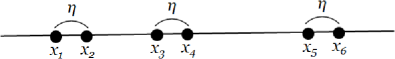
Figure 1: Pairs of RS particles ($N=6$, $N_{0}=3$).

In this section we reproduce the result of [17] and show that the restriction of the RS dynamics of $N=2N_{0}$ particles to the subspace ${\cal P}$ in which the particles stick together in $N_{0}$ pairs such that

$$x_{2i}-x_{2i-1}=\eta,\qquad i=1,\ldots,N_{0}$$ (3.1)

leads to the equations of motion of the deformed RS system for coordinates of the pairs. It is natural to introduce the variables

$$X_{i}=x_{2i-1},\qquad i=1,\ldots,N_{0}$$ (3.2)

which are coordinates of the pairs. It was proved in [17] that such structure is preserved by the ${\sf H}_{1}^{-}$-flow $\partial_{t}=\partial_{t_{1}}-\partial_{\bar{t}_{1}}$ but is destroyed by the ${\sf H}_{1}^{+}$-flow $\partial_{t_{1}}+\partial_{\bar{t}_{1}}$. Therefore, to define the dynamical system we should fix $T_{1}^{+}=\frac{1}{2}\,(t_{1}+\bar{t}_{1})$ to be $0$, i.e. put $\bar{t}_{1}=-t_{1}$, and consider the evolution with respect to the time $t=T_{1}^{-}=\frac{1}{2}\,(t_{1}-\bar{t}_{1})$.

For the velocities $\dot{x}_{i}=\partial{\sf H}_{1}^{-}/\partial p_{i}$ we have:

$$\dot{x}_{2i-1}=e^{p_{2i-1}}\!\prod_{j=1,\neq 2i-1}^{2N_{0}}\!\frac{\sigma(x_{2i-1,j}+\eta)}{\sigma(x_{2i-1,j})}+\sigma^{2}(\eta)e^{-p_{2i-1}}\!\prod_{j=1,\neq 2i-1}^{2N_{0}}\!\frac{\sigma(x_{2i-1,j}-\eta)}{\sigma(x_{2i-1,j})},$$ (3.3)

$$\dot{x}_{2i}=e^{p_{2i}}\!\prod_{j=1,\neq 2i}^{2N_{0}}\!\frac{\sigma(x_{2i,j}+\eta)}{\sigma(x_{2i,j})}\,+\,\sigma^{2}(\eta)e^{-p_{2i}}\!\prod_{j=1,\neq 2i}^{2N_{0}}\!\frac{\sigma(x_{2i,j}-\eta)}{\sigma(x_{2i,j})}.$$ (3.4)

Under the constraint (3.1) the first term in the right hand side of (3.3) vanishes. The second term in the right hand side of (3.4) also vanishes. Then in terms of coordinates $X_{i}$ of the pairs equations (3.3), (3.4) read:

$$\begin{array}[]{l}\displaystyle{\dot{x}_{2i-1}=\sigma(\eta)\sigma(2\eta)e^{-p_{2i-1}}\!\prod_{j=1,\neq i}^{N_{0}}\!\frac{\sigma(X_{ij}-2\eta)}{\sigma(X_{ij})}},\\ \\ \displaystyle{\dot{x}_{2i}=\frac{\sigma(2\eta)}{\sigma(\eta)}\,e^{p_{2i}}\!\prod_{j=1,\neq i}^{N_{0}}\!\frac{\sigma(X_{ij}+2\eta)}{\sigma(X_{ij})}}.\end{array}$$ (3.5)

From (3.5) it is clear that if we set

$$p_{2i-1}=\alpha_{i}+P_{i},\quad p_{2i}=\alpha_{i}-P_{i},\quad i=1,\ldots,N_{0},$$ (3.6)

where

$$\alpha_{i}=\log\sigma(\eta)+\frac{1}{2}\sum_{j\neq i}^{N_{0}}\log\frac{\sigma(X_{ij}-2\eta)}{\sigma(X_{ij}+2\eta)}$$ (3.7)

and $P_{i}$ are arbitrary, then we have $\dot{x}_{2i-1}=\dot{x}_{2i}$ for any $i$, so the distance between the particles in each pair is preserved by the dynamics. Under the ${\sf H}_{1}^{-}$-flow each pair moves as a whole thing. Equations (3.5) are then equivalent to the single equation

$$\dot{X}_{i}=\sigma(2\eta)e^{-P_{i}}\prod_{j\neq i}^{N_{0}}\frac{(\sigma(X_{ij}-2\eta)\sigma(X_{ij}+2\eta))^{1/2}}{\sigma(X_{ij})}.$$ (3.8)

We have passed from the initial $4N_{0}$-dimensional phase space ${\cal F}$ with coordinates $(\{x_{i}\}_{N},\{p_{i}\}_{N})$ to the $2N_{0}$-dimensional subspace ${\cal P}\subset{\cal F}$ of pairs defined by the constraints

$$\left\{\begin{array}[]{l}x_{2i}-x_{2i-1}=\eta,\quad x_{2i-1}=X_{i},\\ \\ \displaystyle{p_{2i-1}+p_{2i}=2\log\sigma(\eta)+\sum_{j\neq i}\log\frac{\sigma(X_{ij}-2\eta)}{\sigma(X_{ij}+2\eta)}}.\end{array}\right.$$ (3.9)

The coordinates in ${\cal P}$ are $(\{X_{i}\}_{N_{0}},\{P_{i}\}_{N_{0}})$.

Proposition 3.1

The space ${\cal P}\subset{\cal F}$ defined by (3.9) is Lagrangian.

Proof. We should prove that the restriction of the canonical 2-form $\displaystyle{\Omega=\sum_{i=1}^{2N}dp_{i}\wedge dx_{i}}$ to the half-dimensional subspace ${\cal P}$ is identically zero. This is a simple calculation with the help of equations (3.6), (3.7) and (3.9).  

Theorem 3.1

The subspace ${\cal P}$ is preserved by the Hamiltonian flow with the Hamiltonian ${\sf H}_{1}^{-}={\sf H}_{1}-\bar{\sf H}_{1}$ and equations of motion of the deformed RS model (1.4) are obtained as the restriction of this flow to the subspace ${\cal P}$.

Proof. Restricting the second set of the Hamiltonian equations, $\dot{p}_{i}=-\partial{\sf H}_{1}^{-}/\partial x_{i}$, to the subspace ${\cal P}$, we have:

$$\begin{array}[]{lll}\dot{p}_{2i-1}&\!\!=\!\!&\displaystyle{\sigma(\eta)\sigma(2\eta)e^{-\alpha_{i}-P_{i}}\!\!\prod_{k=1,\neq i}^{N_{0}}\!\!\frac{\sigma(X_{ik}-2\eta)}{\sigma(X_{ik})}\left[\sum_{j=1,\neq i}^{N_{0}}\Bigl{(}\zeta(X_{ij}\!-\!2\eta)\!-\!\zeta(X_{ij})\Bigr{)}\!+\!\zeta(\eta)\!-\!\zeta(2\eta)\right]}\\ &&\\ &&+\,\displaystyle{\sigma(\eta)\sigma(2\eta)\sum_{l=1,\neq i}^{N_{0}}e^{-\alpha_{l}-P_{l}}\!\prod_{k=1,\neq l}^{N_{0}}\frac{\sigma(X_{lk}-2\eta)}{\sigma(X_{lk})}\Bigl{(}\zeta(X_{il}+\eta)-\zeta(X_{il})\Bigr{)}}\\ &&\\ &&-\,\displaystyle{\frac{\sigma(2\eta)}{\sigma(\eta)}\sum_{l=1}^{N_{0}}e^{\alpha_{l}-P_{l}}\!\prod_{k=1,\neq l}^{n}\frac{\sigma(X_{lk}+2\eta)}{\sigma(X_{lk})}\Bigl{(}\zeta(X_{il}-2\eta)-\zeta(X_{il}-\eta)\Bigr{)}}\\ &&\\ &&+\,\displaystyle{\sigma^{-1}(\eta)e^{\alpha_{i}+P_{i}}\prod_{k=1,\neq i}^{N_{0}}\frac{\sigma(X_{ik}+\eta)}{\sigma(X_{ik})-\eta)}-\sigma(\eta)e^{-\alpha_{i}+P_{i}}\prod_{k=1,\neq i}^{N_{0}}\frac{\sigma(X_{ik}-\eta)}{\sigma(X_{ik})+\eta)}}.\end{array}$$ (3.10)

Taking the time derivative of (3.8), we obtain:

$$\begin{array}[]{l}\displaystyle{\ddot{X}_{i}=-\sigma(2\eta)\dot{P}_{i}e^{-P_{i}}\prod_{j\neq i}^{N_{0}}\frac{(\sigma(X_{ij}-2\eta)\sigma(X_{ij}+2\eta))^{1/2}}{\sigma(X_{ij})}}\\ \\ \displaystyle{+\frac{1}{2}\sum_{j\neq i}^{N_{0}}\dot{X}_{i}(\dot{X}_{i}-\dot{X}_{j})\Bigl{(}\zeta(X_{ij}-2\eta)+\zeta(X_{ij}+2\eta)-2\zeta(X_{ij})\Bigr{)},}\end{array}$$ (3.11)

where we should substitute $\dot{P}_{i}=-\dot{\alpha}_{i}+\dot{p}_{2i-1}$ from (3.10) taking into account (3.8):

$$\dot{P}_{i}=-\dot{\alpha}_{i}+\dot{X}_{i}\left[\sum_{j\neq i}^{N_{0}}\Bigl{(}\zeta(X_{ij}-2\eta)-\zeta(X_{ij})\Bigr{)}+\zeta(\eta)-\zeta(2\eta)\right]$$

$$+\sum_{l\neq i}^{N_{0}}\dot{X}_{l}\Bigl{(}\zeta(X_{il}+\eta)-\zeta(X_{il})\Bigr{)}-\sum_{l=1}^{N_{0}}\dot{X}_{l}\Bigl{(}\zeta(X_{il}-2\eta)-\zeta(X_{il}-\eta)\Bigr{)}$$

$$+e^{P_{i}}\prod_{k\neq i}^{N_{0}}\frac{\sigma^{1/2}(X_{ik}-2\eta)\sigma(X_{ik}+\eta)}{\sigma^{1/2}(X_{ik}+2\eta)\sigma(X_{ik}-\eta)}-e^{P_{i}}\prod_{k\neq i}^{N_{0}}\frac{\sigma^{1/2}(X_{ik}+2\eta)\sigma(X_{ik}-\eta)}{\sigma^{1/2}(X_{ik}-2\eta)\sigma(X_{ik}+\eta)}.$$

Plugging here $\dot{\alpha}_{i}$ from (3.7) and substituting into (3.11), we finally obtain:

$$\ddot{X}_{i}=-\sum_{j\neq i}^{N_{0}}\dot{X}_{i}\dot{X}_{j}\Bigl{(}\zeta(X_{ij}+\eta)+\zeta(X_{ij}-\eta)-2\zeta(X_{ij})\Bigr{)}+\sigma(2\eta)\Bigl{(}U_{i}^{+}-U_{i}^{-}\Bigr{)},$$ (3.12)

where

$$U_{i}^{\pm}=\prod_{j\neq i}^{N_{0}}\frac{\sigma(X_{ij}\pm 2\eta)\sigma(X_{ij}\mp\eta)}{\sigma(X_{ij}\pm\eta)\sigma(X_{ij})}.$$ (3.13)

These are equations (1.1), (1.2) of the deformed RS system (at $g=\sigma(2\eta)$, $N=N_{0}$).  

4 Integrals of motion

In this section we are going to prove that the subspace ${\cal P}$ is invariant not only with respect to the ${\sf H}_{1}^{-}$-flow but also with respect to all higher ${\sf H}_{k}^{-}$-flows. This gives the possibility to obtain integrals of motion $J_{n}$ of the deformed RS model by restriction of the RS integrals of motion ${\sf J}_{n}$, ${\sf J}_{-n}$ to the subspace ${\cal P}$. We denote the restriction of ${\sf J}_{k}$ by $J_{k}$:

$$J_{k}((\{X_{i}\}_{N_{0}},\{P_{i}\}_{N_{0}})={\sf J}_{k}(\{x_{\ell}\}_{N},\{p_{\ell}\}_{N})\Bigr{|}_{{\cal P}},\quad k\in\mbox{\Bbb Z}.$$ (4.1)

The notation ${\sf J}_{k}(\{x_{\ell}\}_{N},\{p_{\ell}\}_{N})\Bigr{|}_{{\cal P}}$ means that the variables $x_{\ell}$, $p_{\ell}$ are constrained by the relations (3.9), i.e.

$$x_{2i-1}=X_{i},\quad x_{2i}=X_{i}+\eta,$$

$$p_{2i-1}=\alpha_{i}(\{X_{j}\}_{N_{0}})+P_{i},\quad p_{2i}=\alpha_{i}(\{X_{j}\}_{N_{0}})-P_{i},$$

where $\alpha_{i}$ is given by (3.7). Note that $J_{k}$ can be regarded as a function of $\{X_{j}\}_{N_{0}}$ and $\{\dot{X}_{j}\}_{N_{0}}$ by virtue of equation (3.8) and

$$\frac{\partial J_{k}}{\partial P_{i}}=-\dot{X}_{i}\frac{\partial J_{k}}{\partial\dot{X}_{i}}.$$

The similar notation will be used for the restriction of the Hamiltonians:

$$\begin{array}[]{l}H_{k}(\{X_{i}\}_{N_{0}},\{P_{i}\}_{N_{0}})={\sf H}_{k}(\{x_{\ell}\}_{N},\{p_{\ell}\}_{N})\Bigr{|}_{{\cal P}},\\ \\ \bar{H}_{k}(\{X_{i}\},\{P_{i}\})=\bar{\sf H}_{k}(\{x_{\ell}\}_{N},\{p_{\ell}\}_{N})\Bigr{|}_{{\cal P}}.\end{array}$$ (4.2)

Theorem 4.1

The space ${\cal P}$ of pairs defined by (3.9) is invariant with respect to the Hamiltonian flows $\partial_{t_{k}}-\partial_{\bar{t}_{k}}$ with the Hamiltonians ${\sf H}_{k}^{-}$ for all $k\geq 1$.

The rest of this section is devoted to the proof of Theorem 4.1. The explicit expressions for integrals of motion of the deformed RS system will follow from the proof.

To prove that the first constraint, $x_{2i-1}-x_{2i}=\eta$, is preserved, we should show that $(\partial_{t_{k}}-\partial_{\bar{t}_{k}})x_{2i-1}=(\partial_{t_{k}}-\partial_{\bar{t}_{k}})x_{2i}$ for all $i=1,\ldots,N_{0}$, i.e. that

$$\frac{\partial{\sf H}_{k}}{\partial p_{2i-1}}-\frac{\partial\bar{\sf H}_{k}}{\partial p_{2i-1}}=\frac{\partial{\sf H}_{k}}{\partial p_{2i}}-\frac{\partial\bar{\sf H}_{k}}{\partial p_{2i}}$$ (4.3)

if the coordinates and momenta are restricted to the space ${\cal P}$. Note that equations (3.6) imply that $\partial_{p_{2i-1}}-\partial_{p_{2i}}=\partial_{P_{i}}$, so (4.3) is equivalent to

$$\frac{\partial H_{k}}{\partial P_{i}}=\frac{\partial\bar{H}_{k}}{\partial P_{i}}.$$ (4.4)

From (2.12) it follows that it is enough to prove that $J_{n}=J_{-n}$.

Let ${\cal N}$ be the set ${\cal N}=\{1,\ldots,N_{0}\}$. Separating the summation in (2.1) over odd and even indexes (with $m$ odd indexes and $n-m$ even ones), we can write, for $0<n\leq N_{0}$:

$$J_{n}=\sum_{m=0}^{n}J_{n,m},$$ (4.5)

where

$$\begin{array}[]{l}\displaystyle{J_{n,m}=\frac{\sigma(n\eta)}{\sigma^{n}(\eta)}\,\sum_{{\cal I},{\cal J}\subseteq{\cal N}\atop{|{\cal I}|=m\atop|{\cal J}|=n-m}}\!\Bigl{(}\prod_{i\in{\cal I}}e^{p_{2i-1}}\Bigr{)}\Bigl{(}\prod_{j\in{\cal J}}e^{p_{2j}}\Bigr{)}}\\ \\ \displaystyle{\times\prod_{\ell\in{\cal N}\setminus{\cal I}}\,\,\prod_{i\in{\cal I}}\frac{\sigma(X_{i\ell}+\eta)}{\sigma(X_{i\ell})}\,\prod_{\ell\in{\cal N}\setminus{\cal I}}\,\prod_{j\in{\cal J}}\frac{\sigma(X_{j\ell}+2\eta)}{\sigma(X_{i\ell}+\eta)}}\\ \\ \displaystyle{\times\prod_{\ell\in{\cal N}\setminus{\cal J}}\,\,\prod_{i\in{\cal I}}\frac{\sigma(X_{i\ell})}{\sigma(X_{i\ell}-\eta)}\,\prod_{\ell\in{\cal N}\setminus{\cal J}}\,\prod_{j\in{\cal J}}\frac{\sigma(X_{j\ell}+\eta)}{\sigma(X_{j\ell})}}.\end{array}$$ (4.6)

Obviously, this is zero unless ${\cal I}\cap({\cal N}\setminus{\cal J})=\emptyset$, i.e. the set ${\cal I}$ should be contained in ${\cal J}$, ${\cal I}\subseteq{\cal J}$. Since $|{\cal I}|=m$, $|{\cal J}|=n-m$, this is possible only if $m\leq[n/2]$, otherwise $J_{n,m}$ vanishes. Using (3.6), (3.7), (3.8), we then have:

$$\Bigl{(}\prod_{i\in{\cal I}}e^{p_{2i-1}}\Bigr{)}\Bigl{(}\prod_{j\in{\cal J}}e^{p_{2j}}\Bigr{)}$$

$$=\frac{\sigma^{n}(\eta)}{\sigma^{n-2m}(2\eta)}\Bigl{(}\prod_{i\in{\cal I}}\,\prod_{\ell\in{\cal N}\setminus\{i\}}\frac{\sigma(X_{i\ell}-2\eta)}{\sigma(X_{i\ell}+2\eta)}\Bigr{)}\,\Bigl{(}\prod_{j\in{\cal J}\setminus{\cal I}}\,\prod_{\ell\in{\cal N}\setminus\{j\}}\frac{\sigma(X_{j\ell})}{\sigma(X_{j\ell}+2\eta)}\Bigr{)}\prod_{j\in{\cal J}\setminus{\cal I}}\dot{X}_{j}.$$

The expression for $J_{-n,m}$ is similar but in this case $m$ is the number of even indexes rather than odd and $\eta$ in all factors in the products should be replaced by $-\eta$. After plugging this into (4.6) and cancellations, we obtain:

$$J_{\pm n,m}=\frac{\sigma(n\eta)}{\sigma^{n-2m}(\eta)}\sum_{{\cal J}\atop|{\cal J}|=n-m}\,\sum_{{\cal I}\subseteq{\cal J}\atop|{\cal I}|=m}\Bigl{(}\prod_{j\in{\cal J}\setminus{\cal I}}\dot{X}_{j}\Bigr{)}\Bigl{(}\prod_{i,j\in{\cal J}\setminus{\cal I}\atop i<j}V(X_{ij})\Bigr{)}\Bigl{(}\prod_{i\in{\cal I}}\prod_{\ell\in{\cal N}\setminus{\cal J}}U^{\pm}(X_{i\ell})\Bigr{)},$$ (4.7)

where

$$V(X_{ij})=\frac{\sigma^{2}(X_{ij})}{\sigma(X_{ij}+\eta)\,\sigma(X_{ij}-\eta)},$$ (4.8)

$$U^{\pm}(X_{ij})=\frac{\sigma(X_{ij}\pm 2\eta)\,\sigma(X_{ij}\mp\eta)}{\sigma(X_{ij}\pm\eta)\,\sigma(X_{ij})}.$$ (4.9)

Passing from summation over the subsets ${\cal J}\subset{\cal N}$ and ${\cal I}\subseteq{\cal J}$ to the summation over subsets ${\cal I}$ and ${\cal I}^{\prime}$ such that ${\cal I}\cap{\cal I}^{\prime}=\emptyset$ (${\cal I}^{\prime}={\cal J}\setminus{\cal I}$), we can write the r.h.s. of (4.7) in the form

$$J_{\pm n,m}=\frac{\sigma(n\eta)}{\sigma^{n-2m}(\eta)}\sum_{{\cal I},{\cal I}^{\prime},{\cal I}\cap{\cal I}^{\prime}=\emptyset\atop|{\cal I}|=m,|{\cal I}^{\prime}|=n-2m}\,\Bigl{(}\prod_{j\in{\cal I}^{\prime}}\dot{X}_{j}\Bigr{)}\Bigl{(}\prod_{i,j\in{\cal I}^{\prime}\atop i<j}V(X_{ij})\Bigr{)}\Bigl{(}\prod_{i\in{\cal I}}\,\prod_{\ell\in{\cal N}\setminus({\cal I}\cup{\cal I}^{\prime})}\!U^{\pm}(X_{i\ell})\Bigr{)}.$$ (4.10)

The equality $J_{n,m}=J_{-n,m}$ is a consequence of the following lemma:

Lemma 4.1

For any ${\cal N}^{\prime}\subseteq{\cal N}=\{1,\ldots,N_{0}\}$ it holds:

$$\sum_{{\cal I}\subset{\cal N}^{\prime}}\prod_{i\in{\cal I}}\prod_{\ell\in{\cal N}^{\prime}\setminus{\cal I}}U^{+}(X_{i\ell})=\sum_{{\cal I}\subset{\cal N}^{\prime}}\prod_{i\in{\cal I}}\prod_{\ell\in{\cal N}^{\prime}\setminus{\cal I}}U^{-}(X_{i\ell}).$$ (4.11)

The lemma is proved in Appendix B. Applying the lemma with ${\cal N}^{\prime}={\cal N}\setminus{\cal I}^{\prime}$ to (4.10), we see that $J_{n,m}=J_{-n,m}$. The formula (1.7) for the integrals of motion in the Introduction is an explicitly symmetrized version of (4.10):

$$J_{n}=\frac{1}{2}\sum_{m=0}^{[n/2]}(J_{n,m}+J_{-n,m}).$$

We have proved the half of the statement of Theorem 4.1: namely, that the first constraint in (3.9), $x_{2i}-x_{2i-1}=\eta$, is invariant under the flows $\partial_{t_{k}}-\partial_{\bar{t}_{k}}$.

Let us prove that the second constraint in (3.9) is preserved too. We should show that the equality in (3.9) remains true after applying $\partial_{t_{n}}-\partial_{\bar{t}_{n}}$ to the both sides. In the l.h.s. we then have

$$\frac{\partial{\sf H}^{-}_{n}}{\partial x_{2i-1}}+\frac{\partial{\sf H}^{-}_{n}}{\partial x_{2i}}=\frac{\partial{\sf H}^{-}_{n}}{\partial X_{i}}.$$

Without loss of generality we may put $i=1$ for simplicity of the notation. Then we have to prove that

$$\frac{\partial{\sf H}^{-}_{n}}{\partial X_{1}}=\sum_{k\neq 1}\left(\frac{\partial{\sf H}^{-}_{n}}{\partial p_{1}}-\frac{\partial{\sf H}^{-}_{n}}{\partial p_{2k-1}}\right)\Bigl{(}\zeta(X_{1k}+2\eta)-\zeta(X_{1k}-2\eta)\Bigr{)}.$$

From (2.12) it is clear that it is equivalent to

$$\frac{\partial{\sf J}^{-}_{n}}{\partial X_{1}}=\sum_{k\neq 1}\left(\frac{\partial{\sf J}^{-}_{n}}{\partial p_{1}}-\frac{\partial{\sf J}^{-}_{n}}{\partial p_{2k-1}}\right)\Bigl{(}\zeta(X_{1k}+2\eta)-\zeta(X_{1k}-2\eta)\Bigr{)}.$$ (4.12)

Repeating the calculation leading to (4.10) for the restriction of $\partial{\sf J}_{\pm n}/\partial p_{2k-1}$ to the subspace ${\cal P}$, we obtain:

$$\frac{\partial{\sf J}_{n}}{\partial p_{2k-1}}=\frac{\sigma(n\eta)}{\sigma^{n-2m}(\eta)}\sum_{m=0}^{[n/2]}\,\sum_{{\cal I}\cap{\cal I}^{\prime}=\emptyset\atop|{\cal I}|=m,\,|{\cal I}^{\prime}|=n-2m}\!\!\Theta(k\in{\cal I})X_{{\cal I}^{\prime}}U_{{\cal I}{\cal I}^{\prime}}^{-},$$ (4.13)

$$\frac{\partial{\sf J}_{-n}}{\partial p_{2k-1}}=\frac{\sigma(n\eta)}{\sigma^{n-2m}(\eta)}\sum_{m=0}^{[n/2]}\,\sum_{{\cal I}\cap{\cal I}^{\prime}=\emptyset\atop|{\cal I}|=m,\,|{\cal I}^{\prime}|=n-2m}\!\!\Theta(k\in{\cal I}\cup{\cal I}^{\prime})X_{{\cal I}^{\prime}}U_{{\cal I}{\cal I}^{\prime}}^{+}.$$ (4.14)

Here

$$X_{{\cal I}^{\prime}}=\Bigl{(}\prod_{j\in{\cal I}^{\prime}}\dot{X}_{j}\Bigr{)}\prod_{j_{1},j_{2}\in{\cal I}^{\prime}\atop j_{1}<j_{2}}V_{j_{1}j_{2}},$$ (4.15)

$$U_{{\cal I}{\cal I}^{\prime}}^{\pm}=\prod_{i\in{\cal I}}\prod_{j\in{\cal N}\setminus({\cal I}\cup{\cal I}^{\prime})}U^{\pm}(X_{ij})$$ (4.16)

and $\Theta(S)$ is the function which is equal to $1$ if the statement $S$ is true and $0$ otherwise. Combining (4.13) and (4.14), we get:

$$\begin{array}[]{l}\displaystyle{\frac{\partial{\sf J}_{n}^{-}}{\partial p_{2k-1}}=\sum_{m=0}^{[n/2]}\kappa_{nm}\left\{\sum_{{\cal I}\cap{\cal I}^{\prime}=\emptyset\atop|{\cal I}|=m,\,|{\cal I}^{\prime}|=n-2m}\!\!\Theta(k\in{\cal I})X_{{\cal I}^{\prime}}\Bigl{(}U_{{\cal I}{\cal I}^{\prime}}^{-}+U_{{\cal I}{\cal I}^{\prime}}^{+}\Bigr{)}\right.}\\ \\ \displaystyle{\left.\phantom{aaaaaaaaaaaaaaa}+\sum_{{\cal I}\cap{\cal I}^{\prime}=\emptyset\atop|{\cal I}|=m,\,|{\cal I}^{\prime}|=n-2m}\!\!\Theta(k\in{\cal I}^{\prime})X_{{\cal I}^{\prime}}U_{{\cal I}{\cal I}^{\prime}}^{+}\right\},}\end{array}$$ (4.17)

where

$$\kappa_{nm}=\sigma(n\eta)\sigma^{2m-n}(\eta).$$ (4.18)

A similar calculation gives

$$\frac{\partial{\sf J}_{\pm n}}{\partial X_{1}}=\sum_{m=0}^{[n/2]}\kappa_{nm}\!\!\!\sum_{{\cal I}\cap{\cal I}^{\prime}=\emptyset\atop|{\cal I}|=m,\,|{\cal I}^{\prime}|=n-2m}\!\!X_{{\cal I}^{\prime}}U_{{\cal I}{\cal I}^{\prime}}^{\mp}Z_{{\cal I}{\cal I}^{\prime}}^{\pm},$$ (4.19)

where

$$\begin{array}[]{c}Z_{{\cal I}{\cal I}^{\prime}}^{+}=\displaystyle{\Theta(1\!\in\!{\cal I})\left(\sum_{\ell\in{\cal N}\setminus({\cal I}\cup{\cal I}^{\prime})}\!\Bigl{(}\zeta(X_{1\ell}+\eta)-\zeta(X_{1\ell}-\eta)\Bigr{)}\!+\!\sum_{\ell\in{\cal I}^{\prime}}\Bigl{(}\zeta(X_{1\ell}+\eta)-\zeta(X_{1\ell})\Bigr{)}\right)}\\ \\ +\displaystyle{\Theta(1\!\in\!{\cal I}\cup{\cal I}^{\prime})\left(\sum_{\ell\in{\cal N}\setminus({\cal I}\cup{\cal I}^{\prime})}\!\Bigl{(}\zeta(X_{1\ell}+2\eta)-\zeta(X_{1\ell})\Bigr{)}\!+\!\sum_{\ell\in{\cal I}^{\prime}}\Bigl{(}\zeta(X_{1\ell}+2\eta)-\zeta(X_{1\ell}+\eta)\Bigr{)}\right)}\\ \\ +\,\displaystyle{\Theta(1\!\in\!{\cal N}\setminus{\cal I})\left(\sum_{\ell\in{\cal I}}\!\Bigl{(}\zeta(X_{1\ell}+2\eta)-\zeta(X_{1\ell})\Bigr{)}\!+\!\sum_{\ell\in{\cal I}^{\prime}}\Bigl{(}\zeta(X_{1\ell}+2\eta)-\zeta(X_{1\ell}+\eta)\Bigr{)}\right)}\\ \\ +\displaystyle{\Theta(1\!\in\!{\cal N}\setminus({\cal I}\cup{\cal I}^{\prime}))\left(\sum_{\ell\in{\cal I}}\!\Bigl{(}\zeta(X_{1\ell}+\eta)-\zeta(X_{1\ell}-\eta)\Bigr{)}\!+\!\sum_{\ell\in{\cal I}^{\prime}}\Bigl{(}\zeta(X_{1\ell}+\eta)-\zeta(X_{1\ell})\Bigr{)}\right)}\end{array}$$ (4.20)

and $Z_{{\cal I}{\cal I}^{\prime}}^{-}$ is obtained from $Z_{{\cal I}{\cal I}^{\prime}}^{+}$ by the change $\eta\to-\eta$. This expression can be brought to a more convenient form by using the obvious relations

$$\Theta(1\!\in\!{\cal I}\cup{\cal I}^{\prime})=\Theta(1\in{\cal I})+\Theta(1\in{\cal I}^{\prime}),\quad\Theta(1\!\in\!{\cal N}\setminus({\cal I})=1-\Theta(1\in{\cal I}).$$

The right hand sides of (4.17) and (4.19) are sums over $m=0,\ldots[n/2]$. Let us denote the $m$th terms of the sums by $\displaystyle{\frac{\partial{\sf J}_{n,m}^{-}}{\partial p_{2k-1}}}$ and $\displaystyle{\frac{\partial{\sf J}_{\pm n,m}^{-}}{\partial X_{1}}}$. We are going to show that

$$\frac{\partial{\sf J}_{n,m}}{\partial X_{1}}-\frac{\partial{\sf J}_{-n,m}}{\partial X_{1}}=\sum_{k\neq 1}\left(\frac{\partial{\sf J}^{-}_{n,m}}{\partial p_{1}}-\frac{\partial{\sf J}^{-}_{n,m}}{\partial p_{2k-1}}\right)\Bigl{(}\zeta(X_{1k}+2\eta)-\zeta(X_{1k}-2\eta)\Bigr{)}$$ (4.21)

from which (4.12) follows. A straightforward calculation yields:

$$\begin{array}[]{c}\displaystyle{\kappa_{nm}^{-1}\left\{\frac{\partial{\sf J}_{n,m}^{-}}{\partial X_{1}}-\sum_{k\neq 1}\left(\frac{\partial{\sf J}^{-}_{n,m}}{\partial p_{1}}-\frac{\partial{\sf J}^{-}_{n,m}}{\partial p_{2k-1}}\right)\Bigl{(}\zeta(X_{1k}+2\eta)-\zeta(X_{1k}-2\eta)\Bigr{)}\right\}}\\ \\ \displaystyle{=\sum_{{\cal I}\cap{\cal I}^{\prime}=\emptyset}X_{{\cal I}^{\prime}}\left\{\Theta(1\in{\cal I})\left[U_{{\cal I}{\cal I}^{\prime}}^{-}{\sum_{\ell}}^{\prime}\zeta^{-}(X_{1\ell})-U_{{\cal I}{\cal I}^{\prime}}^{+}{\sum_{\ell}}^{\prime}\zeta^{+}(X_{1\ell})+U_{{\cal I}{\cal I}^{\prime}}^{+}{\sum_{{\ell}\in{\cal I}}}^{\prime}\zeta^{+}(X_{1\ell})\right.\right.}\\ \\ \displaystyle{+U_{{\cal I}{\cal I}^{\prime}}^{+}{\sum_{{\ell}\in{\cal I}}}^{\prime}\zeta^{-}(X_{1\ell})-U_{{\cal I}{\cal I}^{\prime}}^{-}{\sum_{{\ell}\in{\cal I}}}^{\prime}\zeta^{-}(X_{1\ell})-U_{{\cal I}{\cal I}^{\prime}}^{-}{\sum_{{\ell}\in{\cal I}}}^{\prime}\zeta^{+}(X_{1\ell})}\\ \\ \displaystyle{\phantom{aaa}\left.+U_{{\cal I}{\cal I}^{\prime}}^{+}{\sum_{{\ell}\in{\cal I}^{\prime}}}\zeta^{+}(X_{1\ell})-U_{{\cal I}{\cal I}^{\prime}}^{-}{\sum_{{\ell}\in{\cal I}^{\prime}}}\zeta^{-}(X_{1\ell})\right]}\\ \\ \displaystyle{+\,\,\Theta(1\in{\cal I}^{\prime})\left[U_{{\cal I}{\cal I}^{\prime}}^{+}{\sum_{{\ell}\in{\cal I}}}\zeta^{-}(X_{1\ell})-U_{{\cal I}{\cal I}^{\prime}}^{-}{\sum_{{\ell}\in{\cal I}}}\zeta^{+}(X_{1\ell})\right]}\\ \\ \displaystyle{\left.+\,\sum_{k\neq 1}\Theta(k\in{\cal I})\left[U_{{\cal I}{\cal I}^{\prime}}^{-}\zeta^{+}(X_{1k})-U_{{\cal I}{\cal I}^{\prime}}^{+}\zeta^{-}(X_{1k})\right]\right\},}\end{array}$$ (4.22)

where

$$\zeta^{\pm}(X)=\zeta(X\pm 2\eta)+\zeta(X\mp\eta)-\zeta(X+\pm\eta)-\zeta(X)$$ (4.23)

and $\displaystyle{{\sum_{\ell}}^{\prime}}$ means that $\ell\neq 1$.

Lemma 4.2

The following identity holds:

$$\begin{array}[]{c}\displaystyle{\sum_{{\cal I}}\Theta(1\in{\cal I})\left[U_{{\cal I}{\cal I}^{\prime}}^{-}\sum_{\ell\in{\cal N}\setminus({\cal I}\cup{\cal I}^{\prime})\atop\ell\neq 1}\zeta^{-}(X_{1\ell})-U_{{\cal I}{\cal I}^{\prime}}^{+}\sum_{\ell\in{\cal N}\setminus({\cal I}\cup{\cal I}^{\prime})\atop\ell\neq 1}\zeta^{+}(X_{1\ell})\right.}\\ \\ \displaystyle{\left.-U_{{\cal I}{\cal I}^{\prime}}^{-}\sum_{\ell\in{\cal I},\ell\neq 1}\zeta^{+}(X_{1\ell})+U_{{\cal I}{\cal I}^{\prime}}^{+}\sum_{\ell\in{\cal I},\ell\neq 1}\zeta^{-}(X_{1\ell})\right]}\\ \\ \displaystyle{+\sum_{{\cal I}}\Theta(1\in{\cal I}^{\prime})\left[U_{{\cal I}{\cal I}^{\prime}}^{+}\sum_{\ell\in{\cal I}}\zeta^{-}(X_{1\ell})-U_{{\cal I}{\cal I}^{\prime}}^{-}\sum_{\ell\in{\cal I}}\zeta^{+}(X_{1\ell})\right]}\\ \\ \displaystyle{+\sum_{{\cal I}}\left[U_{{\cal I}{\cal I}^{\prime}}^{-}\sum_{\ell\in{\cal I},\ell\neq 1}\zeta^{+}(X_{1\ell})-U_{{\cal I}{\cal I}^{\prime}}^{+}\sum_{\ell\in{\cal I},\ell\neq 1}\zeta^{-}(X_{1\ell})\right]=0},\end{array}$$ (4.24)

where $U_{{\cal I}{\cal I}^{\prime}}^{\pm}$ and $\zeta^{\pm}(x)$ are defined in (4.16) and (4.23) respectively.

Proof. This is the $X_{1}$-derivative of the identity (4.11) from Lemma 4.1 with ${\cal N}^{\prime}={\cal N}\setminus{\cal I}^{\prime}$.  

Using this identity, it is easy to see that the r.h.s. of (4.22) is zero. Therefore, the invariance of the subspace ${\cal P}$ of pairs with respect to the flows with Hamiltonians ${\sf H}^{-}_{n}$ is proved.

So far we considered the restriction of ${\cal J}_{n}$ with $n<N/2=N_{0}$. The case $N/2<n\leq N$ can be considered in a similar way with the result that the restriction of ${\cal J}_{n}$ with $N_{0}<n\leq 2N_{0}$ is $J_{n-2N_{0}}$. The proof of Theorem 4.1 can be extended to this case, too.

Finally, let us comment on whether the integrals of motion are in involution. As soon as the Hamiltonian structure of the deformed RS system (if any) is not known, we are not able to calculate the Poisson brackets between the integrals of motion and prove that they are equal to zero. Our integrals of motion are functions of coordinates and velocities rather than coordinates and momenta. However, in any integrable system all integrals of motion that are in involution are conserved quantities for the flows generated by any one of them. Each higher Hamiltonian ${\sf H}^{-}_{n}$ of the RS system defines a flow $\partial_{T_{n}^{-}}$ on the “phase space” ${\cal P}$ of the deformed RS system. From the fact that RS integrals of motion are in involution it follows that the restrictions $H_{n}$ of the RS Hamiltonians to the space ${\cal P}$ are conserved under all $\partial_{T_{k}^{-}}$-flows. In this sense we can say that the integrals of motion $H_{n}$ and $J_{n}$ of the deformed RS system are in involution.

5 Generating function of the integrals of motion

It is known that the integrals of motion of the RS system with $2N$ particles can be unified into a generating function which is the determinant of the $2N\!\times\!2N$ matrix $zI-L(\lambda)$, where $I$ is the unity matrix, $z$ is the spectral parameter and $L(\lambda)$ is the Lax matrix depending on another spectral parameter $\lambda$. The Lax matrix has the form

$$L_{ij}(\lambda)=\partial_{t_{1}}x_{i}\,\phi(x_{ij}-\eta,\lambda),$$ (5.1)

where the function $\phi(x,\lambda)$ is given by

$$\phi(x,\lambda)=\frac{\sigma(x+\lambda)}{\sigma(\lambda)\sigma(x)}.$$ (5.2)

Proposition 5.1

([10]) It holds

$$\det_{1\leq i,j\leq 2N}\Bigl{(}z\delta_{ij}-L_{ij}(\lambda)\Bigr{)}=z^{2N}+\sum_{k=1}^{2N}z^{2N-k}\frac{\sigma(\lambda-k\eta)}{\sigma(\lambda)\sigma(k\eta)}\,{\sf J}_{k},$$ (5.3)

where ${\sf J}_{k}$ are the RS integrals of motion (2.9) (see (2.10) with $N\to 2N$).

Proof of this proposition is based on the formula for the determinant of the elliptic Cauchy matrix:

$$\det_{1\leq i,j\leq n}\phi(y_{i}-x_{j})=\frac{\sigma\Bigl{(}\lambda+\sum\limits_{k=1}^{n}(y_{k}-x_{k})\Bigr{)}}{\sigma(\lambda)}\,\frac{\prod\limits_{k<l}\sigma(y_{k}-y_{l})\sigma(x_{l}-x_{k})}{\prod\limits_{k,l}\sigma(y_{k}-x_{l})}.$$ (5.4)

In this section we are going to construct the generating function for the integrals of motion (1.7). The idea is to restrict the Lax matrix (5.1) to the subspace ${\cal P}$. However, the direct restriction is not possible because some matrix elements become infinite. Nevertheless, we shall see that the determinant (5.3) is finite.

To regularize the Lax matrix, we put

$$x_{2i}-x_{2i-1}=\eta+\varepsilon$$ (5.5)

and tend $\varepsilon\to 0$ at the end. At $\varepsilon=0$ we have $\partial_{t_{1}}x_{2i}=\dot{X}_{i}$ and $\partial_{t_{1}}x_{2i-1}=0$. To proceed, we need to find $\partial_{t_{1}}x_{2i-1}$ up to the first non-vanishing order in $\varepsilon$. A simple calculation shows that

$$\partial_{t_{1}}x_{2i-1}=\varepsilon\sigma(2\eta)\dot{X}_{i}^{-1}U_{i}^{-}+O(\varepsilon^{2}),$$ (5.6)

where $U_{i}^{-}$ is given by (3.13) (with $N_{0}\to N$). The further calculation of matrix elements of the Lax matrix is straightforward:

$$\begin{array}[]{l}L_{2i-1,2j-1}:=L_{ij}^{({\rm oo})}=\varepsilon\sigma(2\eta)\dot{X}_{i}^{-1}U_{i}^{-}\phi(X_{ij}-\eta,\lambda)+O(\varepsilon^{2}),\\ \\ L_{2i-1,2j}:=L_{ij}^{({\rm oe})}=\varepsilon\sigma(2\eta)\dot{X}_{i}^{-1}U_{i}^{-}\phi(X_{ij}-2\eta,\lambda)+O(\varepsilon^{2}),\\ \\ L_{2i,2j-1}:=L_{ij}^{({\rm eo})}=\dot{X}_{i}\phi(X_{ij}+\varepsilon,\lambda)+\delta_{ij}O(1)+O(\varepsilon),\\ \\ L_{2i,2j}:=L_{ij}^{({\rm ee})}=\dot{X}_{i}\phi(X_{ij}-\eta,\lambda)+O(\varepsilon).\end{array}$$ (5.7)

After re-numeration of rows and columns, the Lax matrix can be represented as a $2\!\times\!2$ block matrix:

$$L=\left(\begin{array}[]{ll}L_{ij}^{({\rm oo})}&L_{ij}^{({\rm oe})}\\ \\ L_{ij}^{({\rm eo})}&L_{ij}^{({\rm ee})}\end{array}\right),\quad i,j=1,\ldots,N.$$ (5.8)

We see that $L_{ii}^{({\rm eo})}$ is singular as $\varepsilon\to 0$ since $\phi(\varepsilon,\lambda)=\varepsilon^{-1}+O(1)$. Using the formula for determinant of a block matrix, we have:

$$\det(zI-L)=\det\Bigl{(}zI-L^{({\rm oo})}\Bigr{)}\det\Bigl{(}zI-L^{({\rm ee})}-L^{({\rm eo})}(zI-L^{({\rm oo})})^{-1}L^{({\rm oe})}\Bigr{)}.$$

It is easy to see that the right hand side is finite as $\varepsilon\to 0$. In order to find the limit as $\varepsilon\to 0$ we can put $L_{ij}^{({\rm oo})}=0$ and forget about the next-to-leading powers of $\varepsilon$ in other blocks. In this way we find:

$$\lim_{\varepsilon\to 0}\Bigl{(}L^{({\rm eo})}(zI-L^{({\rm oo})})^{-1}L^{({\rm oe})}\Bigr{)}_{ij}=\sigma(2\eta)z^{-1}U_{i}^{-}\phi(X_{ij}-2\eta,\lambda).$$

Therefore, the generating function of integrals of motion is

$$R(z,\lambda)=\det_{1\leq i,j\leq N}\Bigl{(}z\delta_{ij}-\dot{X}_{i}\phi(X_{ij}\!-\!\eta,\lambda)-\sigma(2\eta)z^{-1}U_{i}^{-}\phi(X_{ij}\!-\!2\eta,\lambda)\Bigr{)}.$$ (5.9)

Proposition 5.2

The generating function $R(z,\lambda)$ is given by

$$\begin{array}[]{l}\displaystyle{R(z,\lambda)=z^{N}+z^{-N}\frac{\sigma(\lambda-2N\eta)}{\sigma(\lambda)}}\\ \\ \displaystyle{\phantom{aaaaaaaaaaaaaaa}+\,\sum_{k=1}^{N}z^{N-k}\frac{\sigma(\lambda-k\eta)}{\sigma(\lambda)\sigma(k\eta)}\,J_{k}+\sum_{k=1}^{N-1}z^{k-N}\frac{\sigma(\lambda-2N\eta+k\eta)}{\sigma(\lambda)\sigma(k\eta)}\,J_{-k}},\end{array}$$ (5.10)

where the integrals of motion are

$$J_{\pm k}=\sum_{m=0}^{[k/2]}J_{\pm k,m}$$

and $J_{\pm k,m}$ are given in (4.10).

Sketch of proof. The proof is a lengthy but straightforward calculation which uses the formula for determinant of sum of two matrices and the formula for determinant of the elliptic Cauchy matrix (5.4). Here are some details. First of all, the determinant $\det(I+M)$ is equal to the sum of all diagonal minors of the matrix $M$ of all sizes, including the “empty minor” which is put equal to $1$. After that we encounter the determinants of the form $\det(A_{\cal J}+B_{{\cal J}})$, where $A_{\cal J}$, $B_{{\cal J}}$ are diagonal minors of the matrices $\dot{X}_{i}\phi(X_{ij}\!-\!\eta,\lambda)$, $\sigma(2\eta)z^{-1}U_{i}^{-}\phi(X_{ij}\!-\!2\eta,\lambda)$ of size $n\leq N$ with rows and columns indexed by indexes from a set ${\cal J}=\{j_{1},\ldots,j_{n}\}\subseteq\{1,\ldots,N\}$ ($j_{1}<j_{2}<\ldots<j_{n}\leq N$). The formula for determinant of sum of two matrices states that

$$\det(A_{\cal J}+B_{{\cal J}})=\sum_{{\cal I}\subseteq{\cal J}}\det A^{(B)}_{{\cal J}\setminus{\cal I}},$$

where summation is carried out over all subsets ${\cal I}$ of the set ${\cal J}$ and $A^{(B)}_{{\cal J}\setminus{\cal I}}$ is the matrix $A_{\cal J}$ in which rows numbered by indexes from the set ${\cal I}$ are substituted by the corresponding rows of the matrix $B_{{\cal J}}$. Each $A^{(B)}_{{\cal J}\setminus{\cal I}}$ is an elliptic Cauchy matrix (multiplied by a diagonal matrix), so the determinant of it is known. To see this, we choose in (5.4) $x_{j}=X_{j}$ and

$$\begin{array}[]{l}y_{j}=X_{j}-\eta\;\;\;\mbox{if $j\in{\cal J}\setminus{\cal I}$},\\ \\ y_{j}=X_{j}-2\eta\;\;\;\mbox{if $j\in{\cal I}$}.\end{array}$$

The determinant in (5.9) is represented as a Laurent polynomial in $z$ with coefficients which are sums over sets ${\cal I},\,{\cal I}^{\prime}\subseteq\{1,\ldots,N\}$ such that ${\cal I}\cap{\cal I}^{\prime}=\emptyset$ as in (4.10).  

The characteristic equation

$$R(z,\lambda)=0$$ (5.11)

defines a Riemann surface $\tilde{\Gamma}$ which is a $2N$-sheet covering of the $\lambda$-plane. This Riemann surface is an integral of motion. Any point of it is $P=(z,\lambda)$, where $z,\lambda$ are connected by equation (5.11). There are $2N$ points above each point $\lambda$. It is easy to see from the right hand side of (5.10) that the Riemann surface $\tilde{\Gamma}$ is invariant under the simultaneous transformations

$$\lambda\mapsto\lambda+2\omega,\quad z\mapsto e^{-2\zeta(\omega)\eta}z\quad\mbox{and}\quad\lambda\mapsto\lambda+2\omega^{\prime},\quad z\mapsto e^{-2\zeta(\omega^{\prime})\eta}z.$$ (5.12)

The factor of $\tilde{\Gamma}$ over the transformations (5.12) is an algebraic curve $\Gamma$ which covers the elliptic curve with periods $2\omega,2\omega^{\prime}$. It is the spectral curve of the deformed RS model.

Proposition 5.3

The spectral curve $\Gamma$ admits a holomorphic involution $\iota$ with two fixed points.

Proof. In the previous section it was proved that $J_{-k}=J_{k}$. Therefore, the equation $R(z,\lambda)=0$ is invariant under the involution

$$\iota:(z,\lambda)\mapsto(z^{-1},2N\eta-\lambda),$$ (5.13)

as is easily seen from (5.10). The fixed points lie above the points $\lambda_{*}$ such that $\lambda_{*}=2N\eta-\lambda_{*}$ modulo the lattice with periods $2\omega,2\omega^{\prime}$, i.e. $\lambda_{*}=N\eta-\omega_{\alpha}$, where $\omega_{\alpha}$ is either $0$ or one of the three half-periods $\omega_{1}=\omega$, $\omega_{2}=\omega^{\prime}$, $\omega_{3}=\omega+\omega^{\prime}$. Substituting this into the equation of the spectral curve and taking into account that $J_{-k}=J_{k}$, we conclude that the fixed points are $(\pm 1,N\eta)$ and there are no fixed points above $\lambda_{*}=N\eta-\omega_{\alpha}$ with $\omega_{\alpha}\neq 0$.  

6 Conclusion and open problems

In this paper we have found the complete set of integrals of motion for the deformed RS system with equations of motion (1.4). This provides enough evidence for integrability of the system. Our method was based on the fact that the deformed RS system is equivalent to the dynamical system for pairs of particles in the standard RS model (with even number of particles) moving as whole things so that the distance between particles in each pair is equal to $\eta$, the inverse “velocity of light” in the RS ($=$ relativistic CM) model. Such pairs are preserved by only a “half” of the higher Hamiltonian flows, so we consider only ${\sf H}_{k}^{-}$-flows and put the time variables associated with the ${\sf H}_{k}^{+}$-flows to zero. The configurations in the full phase space ${\cal F}$ when particles stick together in pairs form a half-dimensional subspace ${\cal P}\subset{\cal F}$ and we have proved that this subspace is Lagrangian and invariant under all ${\sf H}_{k}^{-}$-flows. Then integrals of motion for the deformed RS system can be obtained by restricting the known RS integrals of motion to the subspace ${\cal P}$. This job has been done in the present paper.

In the $\eta\to 0$ limit (in which the RS system reduces to the CM system) the particles in each pair turn out to merge in one and the same point. This singular limiting case was discussed in [20].

It is an interesting question whether any clusters of RS particles other than pairs are possible in this sense. For example, one may consider “strings” of $M$ particles such that the coordinates of the particles in the $i$th string are $x_{Mi+1-\alpha}=X_{i}+(M-\alpha)\eta$, $\alpha=1,\ldots,M$, with $X_{i}$ being the coordinate of the string moving as a whole thing. It is natural to ask whether some Hamiltonian flows of the RS model preserve such string structure.

We should stress that the connection between the standard RS system and the deformed RS system is not trivial and has different aspects. On one hand, the latter is an extension of the former and includes it as a particular case because equations of motion (1.4) differ from equations of motion (1.2) of the RS system by presence of some additional terms. However, on the other hand, the deformed RS system is contained in the RS system since it can be regarded as its reduction in the sense that the equations of motion (1.4) are obtained by restriction of the RS dynamics to the subspace ${\cal P}$ of pairs.

Finally, let us list some open problems which arise in connection with the deformed RS system. First, it is important to answer the question whether the deformed RS system is Hamiltonian or not. A related problem is quantization of the deformed RS system. Second, it would be highly desirable to find a commutation representation for equations of motion (1.4) such as Lax representation or Manakov’s triple representation [21]. It is the latter that is known to exist for equations (1.6) which can be obtained from (1.4) in the $\eta\to 0$ limit. That is why it is natural to conjecture that Manakov’s triple representation exists for equations (1.4) for all $\eta\neq 0$. Third, it would be interesting to find Bäcklund transformations of the deformed RS system which are closely connected with the so-called self-dual form of equations of motion and integrable time discretization of them. All this is known to exist for the CM and RS systems (see [22]-[28]). We hope to discuss these problems elsewhere.

Appendix A: The Weierstrass functions

In this appendix we present the definition and main properties of the Weierstrass functions: the $\sigma$-function, the $\zeta$-function and the $\wp$-function which are widely used in the main text.

Let $\omega$, $\omega^{\prime}$ be complex numbers such that ${\rm Im}(\omega^{\prime}/\omega)>0$. The Weierstrass $\sigma$-function with quasi-periods $2\omega$, $2\omega^{\prime}$ is defined by the following infinite product over the lattice $2\omega m+2\omega^{\prime}m^{\prime}$, $m,m^{\prime}\in\mbox{\Bbb Z}$:

$$\sigma(x)=\sigma(x|\,\omega,\omega^{\prime})=x\prod_{s\neq 0}\Bigl{(}1-\frac{x}{s}\Bigr{)}\,e^{\frac{x}{s}+\frac{x^{2}}{2s^{2}}},\quad s=2\omega m+2\omega^{\prime}m^{\prime}\quad m,m^{\prime}\in\mbox{\Bbb Z}.$$ (A1)

It is an odd entire quasiperiodic function in the complex plane. As $x\to 0$,

$$\sigma(x)=x+O(x^{5}),\quad x\to 0.$$ (A2)

The monodromy properties of the $\sigma$-function under shifts by the quasi-periods are as follows:

$$\begin{array}[]{l}\sigma(x+2\omega)=-e^{2\zeta(\omega)(x+\omega)}\sigma(x),\\ \\ \sigma(x+2\omega^{\prime})=-e^{2\zeta(\omega^{\prime})(x+\omega^{\prime})}\sigma(x).\end{array}$$ (A3)

Here $\zeta(x)$ is the Weierstrass $\zeta$-function defined as

$$\zeta(x)=\frac{\sigma^{\prime}(x)}{\sigma(x)}.$$ (A4)

The monodromy properties imply that the function

$$f(x)=\prod_{\alpha=1}^{M}\frac{\sigma(x-a_{\alpha})}{\sigma(x-b_{\alpha})},\qquad\sum_{\alpha=1}^{M}(a_{\alpha}-b_{\alpha})=0$$

is a double-periodic function with periods $2\omega$, $2\omega^{\prime}$ (an elliptic function).

The Weierstrass $\zeta$-function can be represented as a sum over the lattice as follows:

$$\zeta(x)=\frac{1}{x}+\sum_{s\neq 0}\Bigl{(}\frac{1}{x-s}+\frac{1}{s}+\frac{x}{s^{2}}\Bigr{)},\quad s=2\omega m+2\omega^{\prime}m^{\prime}\quad m,m^{\prime}\in\mbox{\Bbb Z}.$$ (A5)

It is an odd function with first order poles at the points of the lattice. As $x\to 0$,

$$\zeta(x)=\frac{1}{x}+O(x^{3}),\quad x\to 0.$$ (A6)

If the argument is shifted by any quasi-period, the $\zeta$-function is transformed as follows:

$$\begin{array}[]{l}\zeta(x+2\omega)=\zeta(x)+\zeta(\omega),\\ \\ \zeta(x+2\omega^{\prime})=\zeta(x)+\zeta(\omega^{\prime}).\end{array}$$ (A7)

These values $\zeta(\omega)$, $\zeta(\omega^{\prime})$ are related by the identity $2\omega^{\prime}\zeta(\omega)-2\omega\zeta(\omega^{\prime})=\pi i$. The transformation properties (A7) imply that the function

$$g(x)=\sum_{\alpha=1}^{M}A_{\alpha}\zeta(x-a_{\alpha}),\qquad\sum_{\alpha=1}^{M}A_{\alpha}=0$$

is an elliptic function.

The Weierstrass $\wp$-function is defined as $\wp(x)=-\zeta^{\prime}(x)$. It can be represented as a sum over the lattice as follows:

$$\wp(x)=\frac{1}{x^{2}}+\sum_{s\neq 0}\Bigl{(}\frac{1}{(x-s)^{2}}-\frac{1}{s^{2}}\Bigr{)},\quad s=2\omega m+2\omega^{\prime}m^{\prime}\quad m,m^{\prime}\in\mbox{\Bbb Z}.$$ (A8)

It is an even double-periodic function with periods $2\omega,2\omega^{\prime}$ and with second order poles at the points of the lattice $s=2\omega m+2\omega^{\prime}m^{\prime}$ with integer $m,m^{\prime}$. As $x\to 0$, $\wp(x)=x^{-2}+O(x^{2})$.

Appendix B: Proof of Lemma 4.1

We set

$$F_{m}^{\pm}=\sum_{{\cal I}\subset{\cal N}^{\prime}\atop|{\cal I}|=m}\prod_{i\in{\cal I}}\prod_{\ell\in{\cal N}^{\prime}\setminus{\cal I}}U^{\pm}(X_{i\ell})=\sum_{{\cal I}\subset{\cal N}^{\prime}\atop|{\cal I}|=m}\prod_{i\in{\cal I}}\prod_{\ell\in{\cal N}^{\prime}\setminus{\cal I}}\frac{\sigma(X_{i\ell}\pm 2\eta)\,\sigma(X_{i\ell}\mp\eta)}{\sigma(X_{i\ell}\pm\eta)\,\sigma(X_{i\ell})}$$ (B1)

and consider the function $f_{m}=F_{m}^{+}-F_{m}^{-}$. It is a symmetric function of the variables $X_{j}$, $j\in{\cal N}^{\prime}$. It is easy to see that it is an elliptic function of each $X_{j}$. The statement of the lemma is that $f_{m}=0$ for all $m$. At $m=1$ we have:

$$f_{1}=\sum_{i\in{\cal N}^{\prime}}\prod_{\ell\in{\cal N}^{\prime}\atop\ell\neq i}\frac{\sigma(X_{i\ell}+2\eta)\,\sigma(X_{i\ell}-\eta)}{\sigma(X_{i\ell}+\eta)\,\sigma(X_{i\ell})}-\sum_{i\in{\cal N}^{\prime}}\prod_{\ell\in{\cal N}^{\prime}\atop\ell\neq i}\frac{\sigma(X_{i\ell}-2\eta)\,\sigma(X_{i\ell}+\eta)}{\sigma(X_{i\ell}-\eta)\,\sigma(X_{i\ell})}=0$$ (B2)

since it is proportional to the sum of residues of the elliptic function

$$f(X)=\prod_{\ell\in{\cal N}^{\prime}}\frac{\sigma(X-X_{\ell}+2\eta)\,\sigma(X-X_{\ell}-\eta)}{\sigma(X-X_{\ell}+\eta)\,\sigma(X-X_{\ell})}.$$

We are going to prove that $f_{m}=0$ for all $m$ by induction. Suppose that $f_{m}=0$ for some $m$; we will show that this is also true for $m\to m+1$. Due to the symmetry, it is enough to consider $f_{m}$ as a function of $X_{1}$ (without loss of generality we assume that ${\cal N}^{\prime}\ni 1$). Possible poles of this function are first order poles at $X_{1}=X_{j}$ and $X_{1}=X_{j}\pm\eta$. Let us prove that residues at these poles actually vanish. For the poles at $X_{1}=X_{j}$ this is especially simple because it is not difficult to see that $\displaystyle{\mathop{\hbox{res}}\limits_{X_{1}=X_{j}}F_{m}^{\pm}=0}$ even without the inductive assumption. Consider the pole at $X_{1}=X_{2}+\eta$ (again, without loss of generality we can assume that ${\cal N}^{\prime}\ni 2$). Let us introduce the short-hand notation ${\cal N}^{\prime}_{1}={\cal N}^{\prime}\setminus\{1\}$, ${\cal N}^{\prime}_{2}={\cal N}^{\prime}\setminus\{2\}$, ${\cal N}^{\prime}_{12}={\cal N}^{\prime}\setminus\{1,2\}$. Then we have:

$$\begin{array}[]{lll}\mathop{\hbox{res}}\limits_{X_{1}=X_{2}+\eta}f_{m}&=&\displaystyle{\sigma(2\eta)\sum_{{\cal I}\subseteq{\cal N}^{\prime}_{12}}\prod_{\ell\in{\cal N}^{\prime}_{12}\setminus{\cal I}}U^{-}(X_{1\ell})\prod_{i\in{\cal I}}\prod_{\ell\in{\cal N}^{\prime}_{1}\setminus{\cal I}}U^{-}(X_{i\ell})}\\ &&\\ &&\phantom{aaaaaa}-\,\displaystyle{\sigma(2\eta)\sum_{{\cal I}\subseteq{\cal N}^{\prime}_{12}}\prod_{\ell\in{\cal N}^{\prime}_{12}\setminus{\cal I}}U^{+}(X_{2\ell})\prod_{i\in{\cal I}}\prod_{\ell\in{\cal N}^{\prime}_{2}\setminus{\cal I}}U^{+}(X_{i\ell})},\end{array}$$ (B3)

where $|{\cal I}|=m-1$. Since $X_{1}=X_{2}+\eta$, we have $U^{+}(X_{2\ell})=U^{-}(X_{1\ell})$. After simple transformations of the products, we can represent (B3) in the form

$$\begin{array}[]{l}\displaystyle{\mathop{\hbox{res}}\limits_{X_{1}=X_{2}+\eta}f_{m}=\sigma(2\eta)\prod_{\ell\in{\cal N}^{\prime}_{12}}\!U^{-}(X_{1\ell})\left[\sum_{{\cal I}\subseteq{\cal N}^{\prime}_{12}}\prod_{i\in{\cal I}}\prod_{\ell\in{\cal N}^{\prime}_{12}\setminus{\cal I}}\!U^{-}(X_{i\ell})-\!\sum_{{\cal I}\subseteq{\cal N}^{\prime}_{12}}\prod_{i\in{\cal I}}\prod_{\ell\in{\cal N}^{\prime}_{12}\setminus{\cal I}}\!U^{+}(X_{i\ell})\right]}\end{array}$$ (B4)

The expression in the square brackets is nothing else than $f_{m-1}$ which is zero by the induction assumption. Therefore, $\displaystyle{\mathop{\hbox{res}}\limits_{X_{1}=X_{2}+\eta}f_{m}=0}$ for all $m$. The pole at $X_{1}=X_{2}-\eta$ and the poles at $X_{1}=X_{j}\pm\eta$ are considered in the similar way. We have shown that the elliptic function $f_{m}$ as a function of $X_{1}$ is regular. Therefore, it does not depend on $X_{1}$. By virtue of the symmetry, this function is a constant which does not depend on all $X_{j}$’s. To find the constant, one may put $X_{j}=\varepsilon j$ and tend $\varepsilon\to 0$. It is easy to see that $f_{m}$ after this substitution is an odd function of $\varepsilon$, so the constant term $\propto\varepsilon^{0}$ in the expansion as $\varepsilon\to 0$ vanishes. This means that the constant is equal to zero.

References

[1]
[2]
F. Calogero, Solution of the one-dimensional
-body problems with quadratic
and/or inversely quadratic pair potentials, J. Math. Phys.
12 (1971) 419–-436.
[3] F. Calogero, Exactly solvable one-dimensional many-body
systems, Lett. Nuovo Cimento 13 (1975) 411–415.
[4]
J. Moser, Three integrable Hamiltonian systems connected with isospectral
deformations, Adv. Math. 16 (1975) 197 –220.
[5] M.A. Olshanetsky and A.M. Perelomov, Classical integrable
finite-dimensional systems related to Lie algebras, Phys. Rep. 71 (1981) 313–400.
[6]
A.M. Perelomov, Completely integrable classical systems
connected with semisimple Lie Algebras, III, Lett. Math. Phys.
1 (1977) 531–534.
[7]
S. Wojciechowski, New completely integrable Hamiltonian systems
of particles on the real line, Phys. Lett. A59 (1977) 84–86.
[8] A.M. Perelomov, Integrable Systems of Classical Mechanics and Lie Algebras,
Birkhäuser Basel, 1990.
[9] S.N.M. Ruijsenaars and H. Schneider, A new class of integrable systems and its relation to
solitons,
Annals of Physics 146 (1986) 1–34.
[10] S.N.M. Ruijsenaars, Complete integrability of
relativistic
Calogero-Moser systems and elliptic function identities,
Commun. Math. Phys. 110 (1987) 191–213.
[11]
H. Airault, H.P. McKean, and J. Moser, Rational and
elliptic solutions of the
Korteweg-De Vries equation and a related many-body problem,
Commun. Pure Appl. Math., 30 (1977) 95–148.
[12]
I.M. Krichever, Rational solutions of the Kadomtsev-Petviashvili
equation and integrable systems of particles on a line,
Funct. Anal. Appl. 12:1 (1978) 59–61.
[13] D.V. Chudnovsky, G.V. Chudnovsky, Pole expansions of non-linear
partial differential equations, Nuovo Cimento 40B (1977) 339–350.
[14] I.M. Krichever, Elliptic
solutions of the Kadomtsev-Petviashvili
equation and integrable systems of particles,
Funk. Anal. i Ego Pril. 14:4 (1980) 45–54
(in Russian); English translation:
Functional Analysis and Its Applications 14:4 (1980) 282–-290.
[15] I. Krichever and A. Zabrodin, Spin generalization of the Ruijsenaars-Schneider model, non-abelian 2D
Toda chain and representations of Sklyanin algebra, Uspekhi Mat. Nauk
50 (1995) 3–56 (in Russian); English translation:
Russ. Math. Surv., 50 (1995) 1101–1150.
[16] V. Prokofev and A. Zabrodin, Elliptic solutions to Toda lattice hierarchy and elliptic
Ruijsenaars-Schneider model,
Teor. Mat. Fys.,
208 (2021) 282–-309 (in Russian);
English translation: Theor. and Math. Phys.,
208 (2021) 1093–1115,
arXiv:2103.00214.
[17]
I. Krichever and A. Zabrodin,
Monodromy free linear equations and many-body systems,
arXiv:2211.17216.
[18]
I. Krichever and A. Zabrodin,
Toda lattice with constraint of type B, arXiv:2210.12534
[19]
D. Rudneva and A. Zabrodin, Dynamics of poles of
elliptic solutions to BKP equation,
Journal of Physics A: Math. Theor. 53 (2020) 075202,
arXiv:1903.00968.
[20]
A. Zabrodin, How Calogero-Moser particles can stick together,
J. Phys. A: Math. Theor. 54 (2021) 225201.
[21] S. Manakov, The method of the
inverse scattering problem
and two-dimensional evolution equations,
Uspekhi Mat. Nauk 31:5 (1976)
245-246.
[22] S. Wojciechowski, The analogue of the
Bäcklund transformation for integrable many-body systems, J. Phys. A:
Math. Gen. 15 (1982) L653-L657.
[23] A. Abanov, E. Bettelheim and P. Wiegmann, Integrable hydrodynamics of Calogero-Sutherland model:
Bidirectional Benjamin-Ono equation,
J. Phys. A 42 (2009) 135201.
[24] G. Bonelli, A. Sciarappa, A. Tanzini and P. Vasko,
Six-dimensional supersymmetric gauge theories, quantum cohomology of
instanton moduli spaces and quantum intermediate long wave hydrodynamics,
JHEP 07 (2014) 141.
[25] A. Zabrodin and A. Zotov,
Self-dual form of Ruijsenaars-Schneider models
and ILW equation with discrete Laplacian,
Nuclear Physics B 927 (2018) 550-565.
[26] F.W. Nihhoff and G.D. Pang, A time-discretized version
of the Calogero-Moser model, Phys. Lett. A 191 (1994) 101-107.
[27] F.W. Nihhoff, O. Ragnisco and V. Kuznetsov,
Integrable time-discretization of the Ruijsenaars-Schneider model,
Commun. Math. Phys. 176 (1996) 681-700.
[28] A. Zabrodin, Elliptic solutions to integrable nonlinear
equations and many-body systems,
Journal of Geometry and Physics 146 (2019) 103506, arXiv:1905.11383.