Covariance-based soft clustering of functional data based on the Wasserstein-Procrustes metric

Abstract

We consider the problem of clustering functional data according to their covariance structure. We contribute a soft clustering methodology based on the Wasserstein-Procrustes distance, where the in-between cluster variability is penalised by a term proportional to the entropy of the partition matrix. In this way, each covariance operator can be partially classified into more than one group. Such soft classification allows for clusters to overlap, and arises naturally in situations where the separation between all or some of the clusters is not well-defined. We also discuss how to estimate the number of groups and to test for the presence of any cluster structure. The algorithm is illustrated using simulated and real data. An R implementation is available in the Supplementary materials.

fourierlargesymbols147

and

1 Introduction

Scientific literature is rich in methods for classifying observations into subsets such that similar observations are clustered together, and dissimilar ones are separated. In this work, we focus on classifying functional observations on the base of their covariance structure. This problem occurs naturally in functional data analysis, for instance, when we are given a collection of $N$ groups of functions in a function space $\mathcal{H}$ (it could be $L^{2}[0,1]$ or a reproducing kernel Hilbert subspace thereof) that manifest different kinds of dispersion around their mean. The functions could arise from bio-physical applications as in Panaretos, Kraus and Maddocks [23], Kraus and Panaretos [19], and Tavakoli and Panaretos [30], where functional curves represent DNA mini-circles; from linguistic applications, where the functional curves represent the spectrograms of spoken phonemes by different speakers (see e.g. Pigoli et al. [27]), and one may wish to classify several groups of sounds; from the analysis of wheel-running activity curves in mice, where one may wish to distinguish several levels of activity evolved across age and generation selections (Cabassi et al. [6]); or again from neuroscience experiments recording sequential trajectories where each trajectory consists of oscillations and fluctuations around zero (Jiao, Frostig and Ombao [15]). What these examples have in common is that it is not the mean structure of the curves that captures the most interesting differences; rather, their (dis)similarities are nested into their second-order structure, embodied by the functional covariance operators.

First-order functional clustering, that is, the clustering of observations based on their mean structure, is a topic widely examined in the literature (see, e.g. the surveys by Jacques and Preda [13], Aneiros et al. [2, Section 2.7], and more pertinent to the scope of this paper, Chamroukhi and Nguyen [8] for model-based clustering). Less literature exists on the classification of covariance operators. Clustering and classifying functional covariances require a way to compare and quantify differences between them, which makes the task more challenging.

Work in this direction can predominantly be found in the multivariate finite dimensional setting, where several methods for clustering covariance matrices exist, especially in connection with statistical shape analysis and diffusion tensor imaging (see, among others, Lee et al. [20] and Srivastava and Klassen [29]). Only recently, methods for classifying infinite-dimensional covariance operators gained some traction. Ieva, Paganoni and Tarabelloni [12] consider differences between global covariance structures limited to the case of two classes of equal size. They focus specifically on a set of observations from two populations who exhibit only second-order variation (same mean, different covariances). Jiao, Frostig and Ombao’s [14] Hilbert–Schmidt based classification is driven by a biomedical (neurological) application. Peng, Rao and Zhao [24] use a covariance dissimilarity measure to classify self-similar stochastic processes when the number of clusters is known, and they later expand it in Peng, Rao and Zhao [25], developing an asymptotically consistent algorithm for classifying of wide-sense stationary ergodic processes.

What the works above have in common is that they measure similarities by embedding covariances in a much larger, linear Hilbert–Schmidt space, and they employ the relative Hilbert–Schmidt (Frobenius) distance. However, covariance operators can essentially be seen as squares of Hilbert–Schmidt operators (Pigoli et al. [26], Masarotto, Panaretos and Zemel [21]), and as such, the space they inhabit is intrinsically non-linear. Although such non-linearity increases the difficulty of the task, properly accounting for it does yield more statistical power. Pigoli et al. [26] and Masarotto, Panaretos and Zemel [21] argue that the Wasserstein-Procrustes distance is the most natural metric that allows to perform statistical analysis on covariance operators, while at the same time respecting their non-linear nature. In this paper, we employ a framework based on the Wasserstein distance of Optimal Transport in order to cluster data with respect to differences in their covariance structure. The Wasserstein framework was recently employed for data clustering in Verdinelli and Wasserman [33]. The authors perform hard distribution clustering with a modified version of the Wasserstein distance and provide successful numerical simulation in dimensions 1 and 2, where they also estimated the number of groups. Kashlak, Aston and Nickl [17] also developed a methodology that accounts for non-linearity and employ an expectation-maximization algorithm to separate curves or operators into $k$ sets via a concentration of measure procedure. They propose an algorithm that updates a vector of probabilities for each operator to belong to a certain cluster until a local optimum is reached. When given the correct number of clusters, their method outperforms standard $k$-means clustering, especially in the highly difficult case of classifying rank 1 operators.

A potential common limitation of the aforementioned methods is that, with the partial exception of Kashlak, Aston and Nickl [17], specialize in hard clustering; that is, each observation is classified in only one group. In contrast, we propose a fuzzy clustering algorithm (referred to as soft clustering in the following) directly based on the Wasserstein-Procrustes distance, in which the in-between cluster variability is penalised by a term proportional to the entropy of the partition matrix. The algorithm characterizes each group using a centroid covariance operator, and simultaneously estimates the degree to which the observed covariances belong to each cluster. Soft classification algorithms resemble model-based clustering, which are techniques that rely on the underlying assumption that the data come from a mixture of distributions (Fraley and Raftery [9]). However, the estimated membership grades do not have a precise probabilistic interpretation, because soft-clustering is not based on any stringent probabilistic assumption. Unlike $k$-means and other hard clustering methods, soft clustering is particularly meaningful in cases in which the cluster separation is not neat, and a soft classification, which allows for overlapping clusters, might be appropriate. Furthermore, it allows us to easily identify the groups that are most confused with each other. We also attempt to ameliorate some of the intrinsic weaknesses of related works by (a) proposing an easy adaptation of the methodology that supports fast clustering when the number of covariance operators is very large and (b) offering insights into how to determine the most suitable number of clusters. Almost all the works previously described require in fact the number of clusters to be known in advance. We introduce a novel cluster quality index, coined Trimmed Average Silhouette Width (TASW), which provides an attractive alternative to the well-known Average Silhouette Width (Rousseeuw [28]) in the case of overlapping clusters and shows extremely good performances in the applications presented. Moreover, the TASW may also be used to test the null hypothesis of whether any cluster is present. Finally, we also aim to fill what, to the best of our knowledge, is a gap in the field: the lack of ready-made, easy-to-use clustering code.

The structure of the paper is as follows. After introducing some basic notions and notations in Section 2, we describe the proposed soft clustering approach in Section 3. In particular, in Section 3, we discuss the methodology, the computational details (also for large datasets), and a cluster quality index that we have found to be useful for selecting the number of groups. In Section 4, we illustrate the usefulness of the procedure on simulated data, as well as two real datasets. Conclusions and some ideas for future research are presented in Section 5. An R implementation of our algorithm is given in the supplementary materials together with an R script that allows to reproduce part of one of the examples in Section 4.

2 Background

2.1 Basic notions and notations

Let $\mathcal{H}$ be a real separable Hilbert space, often taken as $L^{2}[0,1]$, with the inner product $\langle\cdot,\cdot\rangle:\mathcal{H}\times\mathcal{H}\rightarrow\mathbb{R}$, and induced norm $\|\cdot\|:\mathcal{H}\to[0,\infty)$. Furthermore, let $\{X_{1,j}\}_{j=1}^{n_{1}},\dots,\{X_{N,j}\}_{j=1}^{n_{N}}$ be $N$ independent samples of i.i.d. random elements in $\mathcal{H}$, possessing, for $i=1,\ldots,N$, well-defined mean functions $\mu_{i}=E\bigl{\{}X_{i,j}\bigr{\}}$ and covariance operators $\Sigma_{i}=E\bigl{\{}(X_{i,j}-\mu_{i})\otimes(X_{i,j}-\mu_{i})\bigr{\}}$, where $\otimes$ stands for the outer product on $\mathcal{H}$. With this notation, we assume that the data might arise from $N$ functional populations modelled by a prototypical random function $X_{i}$, and that we are able to observe $n_{i}>1$ realisations from each population. Populations might differ in both mean and covariance structure. However, as previously mentioned, we assume that the scientific interest concerns the differences in the covariance operators.

We say that a (possibly unbounded) operator $A$ is self-adjoint if $\langle Au,v\rangle=\langle u,Av\rangle$ for all $u$ and $v$ in the domain of definition of $A$. If $A$ also happens to be bounded, then this is equivalent to the condition that $A=A^{*}$, where $A^{*}$ denotes the adjoint operator. A non-negative operator is a self-adjoint operator $A$ such that $\langle Au,u\rangle\geq 0$ for all $u$ in the domain of $A$. In addition, if $A$ is compact, then there exists a unique non-negative self-adjoint operator whose square equals $A$, which is denoted by either $A^{1/2}$ or $\sqrt{A}$. The inverse square root $(A^{1/2})^{-1}$ is denoted by $A^{-1/2}$. The inverse may not be defined or defined only on a (dense) subspace of $\mathcal{H}$. For any bounded operator $A$, $A^{*}A$ is non-negative. The identity operator on $\mathcal{H}$ is denoted by $\mathscr{I}$.

In this setting, covariances are linear operators from $\mathcal{H}$ into $\mathcal{H}$, which are self-adjoint, non-negative, and trace-class, meaning that their nuclear norm $\big{\hsnorm}A\big{\hsnorm}_{1}={\rm tr}\sqrt{A^{*}A}$, with ${\rm tr}$ denoting the trace operator, is bounded away from infinity. Thus, a covariance operator $\Sigma$ on $\mathcal{H}$ can be considered the “square” of a Hilbert–Schmidt operator: If $\big{\hsnorm}A\big{\hsnorm}_{2}=\sqrt{{\rm tr}A^{*}A}<\infty$, then $A$ is certainly bounded, and $\Sigma=A^{*}A$ defines a valid covariance operator. Viewing covariances as squares highlights their non-linear nature, and any method for measuring (dis)similarities should account for this non-linearity.

2.2 On the choice of a suitable distance

A classical strategy for dealing with non-linearity in infinite dimension has been embedding covariances in a much larger, linear Hilbert-Schmidt space, and comparing them directly by means of the Hilbert-Schmidt distance $\big{\hsnorm}\Sigma_{1}-\Sigma_{2}\big{\hsnorm}_{2}=\sqrt{{\rm tr}(\Sigma_{1}-\Sigma_{2})^{*}(\Sigma_{1}-\Sigma_{2})}$ (Panaretos, Kraus and Maddocks [23], Fremdt et al. [11], Boente, Rodriguez and Sued [5]). However, Pigoli et al. [26] showed that there exists a much more natural metric that respects the non-linear nature of covariances while being well-defined in infinite dimensions, that is, the so-called Procrustes metric

$$\Pi(\Sigma_{1},\Sigma_{2})=\inf_{U^{*}U=\mathscr{I}}\big{\hsnorm}\Sigma^{1/2}_{1}-\Sigma^{1/2}_{2}U\big{\hsnorm}_{2}.$$

Masarotto, Panaretos and Zemel [21] further developed several key properties of this metric and its geometry. Their development leverages the observation that two covariance operators $\Sigma_{1}$ and $\Sigma_{2}$ can be bijectively identified with two centered Gaussian measures $N(0,\Sigma_{1})$ and $N(0,\Sigma_{2})$ on the Hilbert space $\mathcal{H}$. The Procrustes metric can then be interpreted via the optimal transportation of Gaussian processes, and identified with the $L^{2}$-Wasserstein distance between the two Gaussian measures.

The Wasserstein distance between two Borel probability measures $\mu$ and $\nu$, both on $\mathcal{H}$, is defined as

$$W^{2}(\mu,\nu)=\inf_{\pi\in\Gamma(\mu,\nu)}{\int_{\mathcal{H}\times\mathcal{H}}\!\|x-y\|^{2}\,\mathrm{d}\pi(x,y)},$$

where the infimum is taken over the set $\Gamma(\mu,\nu)$ of all the couplings of $\mu$ and $\nu$. Alternatively,

$$W^{2}(\mu,\nu)=\inf_{(Z_{1},Z_{2})}\mathbb{E}\|Z_{1}-Z_{2}\|^{2},$$

where the infimum is over all random vectors $(Z_{1},Z_{2})$ in $\mathcal{H}\times\mathcal{H}$ such that $Z_{1}\sim\mu$ and $Z_{2}\sim\nu$, marginally. The distance is finite when $\mu$ and $\nu$ have a finite second moment. The optimisation problem above is known as the Monge–Kantorovich problem of optimal transportation. If $\mu$ and $\nu$ are Gaussian measures $N(0,\Sigma_{1})$ and $N(0,\Sigma_{2})$, then the Wasserstein distance can be expressed in closed form as

$$W^{2}(\mu,\nu) =\Pi^{2}(\Sigma_{1},\Sigma_{2})=\inf_{\begin{smallmatrix}Z_{1}\sim N(0,\Sigma_{1})\\ Z_{2}\sim N(0,\Sigma_{2})\end{smallmatrix}}\mathbb{E}\|Z_{1}-Z_{2}\|^{2}$$

$$={\rm tr}\Sigma_{1}+{\rm tr}\Sigma_{2}-2{\rm tr}\sqrt{\Sigma_{1}^{1/2}\Sigma_{2}\Sigma_{1}^{1/2}}.$$

2.3 Weighted Fréchet means/Wasserstein barycenters

If $\Sigma_{1},\dots,\Sigma_{N}$ are covariance operators, and $\pi_{1},\ldots,\pi_{N}$ are non-negative weights, their (weighted) Fréchet mean (Fréchet [10]) with respect to the Procrustes metric (or equivalently, their Wasserstein barycenter of the corresponding centred Gaussian measures) is defined as the minimiser of the Fréchet functional

$$F(\Sigma)=\sum_{i=1}^{N}\pi_{i}\Pi^{2}(\Sigma_{i},\Sigma)=\sum_{i=1}^{N}\pi_{i}W^{2}\bigl{(}N(0,\Sigma_{i}),N(0,\Sigma)\bigr{)}.$$

Unlike the finite dimension case, the existence and uniqueness of Fréchet means in general metric space is not guaranteed (see, e.g., Karcher [16]). In Wasserstein spaces, however, these can be established under rather mild assumptions thanks to the notion of optimal multicoupling (Masarotto, Panaretos and Zemel [21]). In particular, any collection $\Sigma_{1},\dots,\Sigma_{N}$ of covariance operators admits a Fréchet mean $\overline{\Sigma}$ with respect to the Procrustes distance $\Pi$ which is stable under finite dimensional projections. For Gaussian measures, it is uniquely defined, and is a Gaussian measure itself (see Agueh and Carlier [1]).

There is no closed-form formula that returns the Fréchet mean $\overline{\Sigma}$, but as described, for example, in Masarotto, Panaretos and Zemel [21, Section 8], it can be iteratively approximated using the following algorithm.

Initialization.

Set $j=0$ and $\overline{\Sigma}^{0}$ equal to an initial guess of the Fréchet mean (e.g., $\overline{\Sigma}^{0}=\sum_{i=1}^{N}\pi_{i}\Sigma_{i}/\sum_{i=1}^{N}\pi_{i}$).

Computation.

Until a suitable convergence criterion is met (or a maximum number of iterations is reached), repeat

• Compute the next iterate as $\overline{\Sigma}^{j+1}=\overline{T}_{j}\overline{\Sigma}^{j}\overline{T}_{j}$ where

  $$\overline{T}_{j}=\left(\sum_{i=1}^{N}\pi_{i}T_{i,j}\right)/\left(\sum_{i=1}^{N}\pi_{i}\right)$$

  with

  $$T_{i,j}=\left(\overline{\Sigma}^{j}\right)^{-1/2}\left[\left(\overline{\Sigma}^{j}\right)^{1/2}\Sigma_{i}\left(\overline{\Sigma}^{j}\right)^{1/2}\right]^{1/2}\left(\overline{\Sigma}^{j}\right)^{-1/2}\;\;(i=1,\ldots,N).$$

• Set $j=j+1$

Output.

Use the final iterate $\overline{\Sigma}^{j}$ as an estimate of $\overline{\Sigma}$.

Note that $T_{i,j}$ is a self-adjoint operator that transports $\overline{\Sigma}^{j}$ to $\Sigma_{i}$, in the sense that $\Sigma_{i}=T_{i,j}\overline{\Sigma}^{J}T_{i,j}$. In terms of the manifold-like geometry of covariances under the Wasserstein-Procrustes metric, the algorithm starts with an initial guess of the Fréchet mean. It then lifts all the covariances to the tangent space at that initial guess, averages linearly on the tangent space, and retracts this average onto the manifold. This retraction is the guess in the following step. The previous algorithm can also be viewed as an implementation of the steepest descent concept in the space of covariances endowed with the Wasserstein-Procrustes metric (Zemel and Panaretos [35], Masarotto, Panaretos and Zemel [21]).

2.4 Finite-dimensional behaviour

In applications such as those presented in Section 4, we inevitably work with finite-dimensional representations of the covariance operators. However, as discussed in Pigoli et al. [26] and Masarotto, Panaretos and Zemel [22], the Wasserstein-Procrustes distance between two finite-dimensional representations provides a good approximation of the corresponding distance between the infinite-dimensional operator. In addition, Masarotto, Panaretos and Zemel [22] established the numerical stability of the Wasserstein barycenters.

3 Soft clustering of covariance operators

3.1 Generalities

As previously mentioned, assume that

• we have observed $N$ independent samples, each of size $n$, of functional data $\{X_{1,j}\}_{j=1}^{n_{1}},\dots,\{X_{N,j}\}_{j=1}^{n_{N}}$;

• we wish to cluster the corresponding covariances $\Sigma_{i}$, $i=1,\ldots,N$, in $K$ groups.

In practice, we have $N$ estimated operators $\widehat{\Sigma}_{1},\ldots,\widehat{\Sigma}_{N}$, for example, the sample covariances defined by

$$\widehat{\Sigma}_{i}=\dfrac{1}{n_{i}-1}\sum_{j=1}^{n_{i}}\bigl{(}X_{i,j}-\widehat{\mu}_{i}\bigr{)}\otimes\bigl{(}X_{i,j}-\widehat{\mu}_{i}\bigr{)}\text{ where }\widehat{\mu}_{i}=\dfrac{1}{n_{i}}\sum_{j=1}^{n}X_{i,j},$$

and we aim to determine

• $K$ prototype covariance operators $\overline{\Sigma}_{1},\ldots,\overline{\Sigma}_{K}$ representative of the $K$ groups; and

• a $N\times K$ (soft) partition matrix

  $$P=[\pi_{i,j}]\text{ such that }\pi_{i,j}\geq 0\text{ and }\sum_{j=1}^{K}\pi_{i,j}=1,$$

  where each element $\pi_{i,j}$ describes the confidence with which the covariance $\widehat{\Sigma}_{i}$ can be assigned to the $j$th group.

A natural scenario would see the $j$th cluster barycenter $\overline{\Sigma}_{j}$ be the Fréchet means of the sample covariances with weights proportional to the membership grades $\pi_{1,j},\ldots,\pi_{N,j}$ and to the sample sizes $n_{1},\ldots,n_{N}$; simultaneously the grades $\pi_{i,j}$ should be determined so that they are close to one when $\widehat{\Sigma}_{i}$ is near $\overline{\Sigma}_{j}$, and close to zero when $\widehat{\Sigma}_{i}$ looks like an outlier for the group identified by $\overline{\Sigma}_{j}$. However, we also recognize that not all the operators have a clear-cut attribution to one of the groups, and with the aim of identifying them and reducing their influence in the barycenters computation, we let $\pi_{i,j}$ assume any value between zero and one.

In particular, the proposed soft clustering method computes $\overline{\Sigma}_{1},\ldots,\overline{\Sigma}_{K}$ and $P$ minimizing

$$\sum_{i=1}^{N}\sum_{j=1}^{K}\pi_{i,j}\bigl{(}n_{i}-1\bigr{)}\Pi^{2}\bigl{(}\widehat{\Sigma}_{i},\overline{\Sigma}_{j}\bigr{)}$$ (1)

subject to the constraints

$$\pi_{i,j}\geq 0\;\;(i=1,\ldots,N\text{ and }j=1,\ldots,K),$$ (C1)

$$\sum_{j=1}^{K}\pi_{i,j}=1\;\;(i=1,\ldots,N),$$ (C2)

$$-\dfrac{1}{N} \sum_{i=1}^{N}\sum_{j=1}^{K}\pi_{i,j}\log\pi_{i,j}=E,$$ (C3)

where $E$ is a user-defined value ($0\leq E\leq\log K$).

The objective function (1), given by the weighted sum of the Wasserstein-Procrustes distances, measures the heterogeneity within the classes, while the constraint (C3) prescribes the desired average level of entropy of the resulting soft classification. In particular, observe that

• when $E=0$ (null average entropy), the constraint can be satisfied only by standard (or hard) partition matrices such that, for every $i$,

  $$\pi_{i,j}=\begin{cases}0,&j\neq r_{i}\\ 1,&j=r_{i}\end{cases}$$ (2)

  for some $r_{i}\in\{1,\ldots,k\}$.

• when $E=\log K$ (maximum average entropy), the constraint implies the non-informative partition matrix

  $$\pi_{i,j}=\dfrac{1}{K}\;\;(i=1,\ldots,N;\;j=1,\ldots,K).$$ (3)

• when $0<E<\log K$, the rows of the resulting partition matrix will neither degenerate as in (2) nor become uniform as in (3).

In the following subsections, we discuss the computation of the soft cluster solution (Subsection 3.2); the choice of the average entropy $E$ (Subsection 3.3); an index, the trimmed average silhouette width, that can be used for selecting suitable values for $K$ (Subsection 3.4); and a simple adaptation of our approach to the “large $N$” scenario (Subsection 3.5).

3.2 Computation of the soft clustering solution

The following proposition, whose proof is sketched in the appendix, naturally leads to the algorithm we implemented for computing the cluster barycenters $\overline{\Sigma}_{1},\ldots,\overline{\Sigma}_{K}$ and the partition matrix $P$.

Proposition.

In the previously described setting

• given the partition matrix $P$, the desired covariance matrices/cluster barycenters $\overline{\Sigma}_{j}$, $j=1,\ldots,K$, are the Fréchet means of $\widehat{\Sigma}_{1},\ldots,\widehat{\Sigma}_{N}$ with weights $(n_{1}-1)\pi_{1,j},\ldots,(n_{N}-1)\pi_{N,j}$, i.e.,

  $$\overline{\Sigma}_{j}=\arg\min_{\Omega}\sum_{i=1}^{N}\pi_{i,j}\bigl{(}n_{i}-1\bigr{)}\Pi^{2}\bigl{(}\widehat{\Sigma}_{i},\Omega\bigr{)};$$ (4)

• given $\overline{\Sigma}_{j}$, $j=1,\ldots,K$, the partition matrix that minimizes (1) under the constraints (C1)–(C3) is

  $$P=\bigl{[}\pi_{i,j}(\widehat{\eta})\bigr{]}$$ (5)

  where

  $$\pi_{i,j}(\eta)=\dfrac{e^{-(n_{i}-1)\Pi^{2}(\widehat{\Sigma}_{i},\overline{\Sigma}_{j})/\eta}}{\sum_{s=1}^{K}e^{-(n_{i}-1)\Pi^{2}(\widehat{\Sigma}_{i},\overline{\Sigma}_{s})/\eta}},$$ (6)

  and $\widehat{\eta}$ denotes the unique positive root of the equation

  $$-\sum_{i=1}^{N}\sum_{j=1}^{K}\pi_{i,j}(\eta)\log\pi_{i,j}(\eta)=NE.$$ (7)

  In addition, the left side of (7) is differentiable and monotone increasing when $\eta>0$. Thus, the computation of $\widehat{\eta}$ is a stable, and essentially trivial, numerical problem.

The result motivates the use of the block coordinate descent algorithm (e.g., Xu and Yin [34]) described in Subsection 3.2.2. The algorithm, which resembles the classical EM approach for fitting mixture models (and model-based clustering), finds only a local minimum of the objective function (1). Thus, it is important to choose a suitable starting point so that this local minimum corresponds to a “good” solution. With this aim, and inspired by the initialisation phase of the kmeans++ (Vassilvitskii and Arthur [32]) and PAM (Kaufman and Rousseeuw [18]) algorithms, we suggest the initialization approach described in Subsection 3.2.1.

3.2.1 Initialisation

During the initialization phase, we try to minimize the sum of the within-group distances (1) adding to the constraints (C1)–(C3) the additional restriction that the group prototypes are equal to some of the observed sample covariances. Therefore, we try to determine the indices $(i_{1},\ldots,i_{K})\in\{1,\ldots,N\}^{K}$ that minimize

$$G(i_{1},\ldots,i_{K})=\sum_{i=1}^{N}\sum_{j=1}^{K}\pi_{i,j}(\widehat{\eta})\bigl{(}n_{i}-1\bigr{)}\Pi^{2}\bigl{(}\widehat{\Sigma}_{i},\widehat{\Sigma}_{i_{j}}\bigr{)}$$

with $\widehat{\eta}$ and $\pi_{i,j}(\widehat{\eta})$ computed as in the previous proposition assuming that $\overline{\Sigma}_{1}=\widehat{\Sigma}_{i_{1}},\ldots,\overline{\Sigma}_{K}=\widehat{\Sigma}_{i_{K}}$. Restricting the search to the observed sample covariances avoids the computing of the Fréchet means, as this is the most time-consuming part of the algorithm described in the next Subsection. As the exact determination of the optimal subset $(i_{1},\ldots,i_{K})$ is not computationally feasible (at least when $N$ is large), we suggest the use of the following stochastic search approach:

1. Repeat nstart times the following steps and keep the best subset $(i_{1},\ldots,i_{K})$ generated.

   1. Choose $i_{1}$ uniformly at random in $\{1,\ldots,N\}$.

   2. For $j=2,\ldots,K$, sequentially choose $i_{j}$ from $\{1,\ldots,N\}$ with probability proportional to $\min\bigl{\{}\Pi^{2}(\widehat{\Sigma}_{i},\widehat{\Sigma}_{i_{1}}),\ldots,\Pi^{2}(\widehat{\Sigma}_{i},\widehat{\Sigma}_{i_{j-1}})\bigr{\}}$.

   3. Repeat nrefine times the following step.

      1. For each $j=1,\ldots,K$, sample without replacement from $\{1,\ldots,N\}$ ntry possible substitutions of $i_{j}$ with probability proportional to $\min_{s\neq j}\Pi^{2}(\widehat{\Sigma}_{i},\widehat{\Sigma}_{i_{s}}).$ Keep the best found value for $i_{j}$.

The algorithm described above is based on the idea that if $i_{a}$ and $i_{b}$ belong to $\{i_{1},\ldots,i_{K}\}$ then the distance $\Pi^{2}(\widehat{\Sigma}_{i_{a}},\widehat{\Sigma}_{i_{b}})$ is expected to be large. Repeated simulations showed that if $K$ groups really exist, this initialisation tends to select covariances $\widehat{\Sigma}_{i_{1}},\dots,\widehat{\Sigma}_{i_{K}}$ belonging to different groups, at least when nstart and nrefine are greater than, or equal, to $5$, and ntry is about $N/K$.

3.2.2 Block coordinate descent algorithm

The local search follows directly from the given proposition. The algorithm starts from the $K$ prototype covariance matrices $\widehat{\Sigma}_{i_{1}},\ldots,\widehat{\Sigma}_{i_{K}}$ selected during the initialization phase and then seeks the solution to the soft cluster problem through iteration of the following two steps until convergence:

1. Given the current estimates of the cluster barycenters, compute the optimal partition matrix from (5)–(7).

2. Given the current partition matrix, update the $K$ prototype covariance matrices using the gradient descent algorithm for the Fréchet mean (see Subsection 2.3).

The algorithm stops when the difference between the sum of the within-class distances (1) in two consecutive iterations is sufficiently small.

3.3 On the choice of the average entropy $E$

In general, $E$ should be chosen based on the the expected average degree of confusion between the clusters. In practice, we obtained good results by setting

$$E=-\bigl{(}1-\alpha\bigl{)}\bigl{[}\beta\log\beta+(1-\beta)\log(1-\beta)\bigr{]}+\alpha\log 2$$ (8)

for positive small values of $\alpha$ and $\beta$ (e.g., we used $\alpha=0.25$ and $\beta=0.05$ in all the applications presented in Section 4). The rationale behind (8) is that, in general, we expect

• most of the sample covariances (say $100(1-\alpha)\%$ of them) to be classified essentially in one group (denote it with $r_{i}$), with some uncertainty about another group ($s_{i}$) ; a prototypical partition matrix row for these cases is

  $$\pi_{i,j}=\begin{cases}1-\beta&\text{if }j=r_{i}\\ \beta&\text{if }j=s_{i}\\ 0&\text{otherwise}\end{cases}.$$

• the remaining small number of sample covariances ($100\alpha\%$) to be confused between two possible overlapping clusters ($r_{i}$ and $s_{i}$); for these cases, a prototypical row of $P$ is

  $$\pi_{i,j}=\begin{cases}\dfrac{1}{2}&\text{if }j\in\{r_{i},s_{i}\}\\ 0&\text{otherwise}\end{cases}.$$

Of course, we do not expect any rows of $P$ to be exactly equal to the previous prototypical rows, but at least in our experience, the use of (8) makes it easy to specify a suitable value for the average entropy.

3.4 Trimmed average silhouette width

In the standard multivariate framework, many cluster quality indexes have been proposed, in particular, with the aim of determining a suitable value for the number of clusters. One popular index is the average silhouette width proposed by Rousseeuw [28], which achieved very good results in Arbelaitz et al.’s [3] extensive study, in which $30$ different indexes were compared. This criterion has been considered not only for choosing an optimal value of $K$ but also for obtaining good partitions for a fixed value of $K$ (see Van der Laan, Pollard and Bryan [31], Batool and Hennig [4]).

As the silhouette width is a widely used intuitive measure of cluster validity, we explored a simple adaptation of the idea to our framework with the aim of providing a tool that can suggest “good” values for the number of cluster $K$, and if desired, is usable to test for the presence of any cluster, that is, the null hypothesis that $K=1$.

Assume that we have computed the soft cluster solutions for $K=2,\ldots,K_{max}$, all using the same average entropy $E$, and denote the membership grades with $\pi_{i,j}^{K}$ and the cluster barycenters with $\overline{\Sigma}_{j}^{K}$, $i=1,\ldots,N$ and $j=1,\ldots,K$. We define the silhouette width of the $i$th sample covariance $\widehat{\Sigma}_{i}$ with respect to the solutions based on $K$ clusters as

$$SW_{i}^{K}=1-\dfrac{\Pi\bigl{(}\widehat{\Sigma}_{i},\overline{\Sigma}_{i_{a}^{K}}^{K}\bigr{)}}{\Pi\bigl{(}\widehat{\Sigma}_{i},\overline{\Sigma}_{i_{b}^{K}}^{K}\bigr{)}},$$ (9)

where $\overline{\Sigma}_{i_{a}^{K}}^{K}$ and $\overline{\Sigma}_{i_{b}^{K}}^{K}$ are the nearest and second nearest barycenters to $\widehat{\Sigma}_{i}$, that is,

$$i_{a}^{K}=\arg\min_{j}\Pi\bigl{(}\widehat{\Sigma}_{i},\overline{\Sigma}_{j}^{K}\bigr{)}\text{ and }i_{b}^{K}=\arg\min_{j\neq i_{a}^{K}}\Pi\bigl{(}\widehat{\Sigma}_{i},\overline{\Sigma}_{j}^{K}\bigr{)}.$$

Intuitively, $SW_{i}^{K}$ measures how well the $i$th sample covariance can be classified in the cluster identified by the nearest barycenter with respect to the second best classification. Observe that our definition of $SW_{i}^{K}$ is analogous to the fast silhouette definition considered by Van der Laan, Pollard and Bryan [31]. With respect to the original definition given by Rousseeuw [28], (9) offers the advantage of requiring only quantities already computed during the computation of the soft cluster solution.

The average silhouette width considered in the literature is the mean of the individual silhouettes $SW_{i}^{K}$, that is, $ASW^{K}=\sum_{i=1}^{N}SW_{i}^{K}/N$. However, this index is not completely appropriate in the framework considered in this paper, because we a priori accept the idea that clusters might overlap, and therefore, that some of the individual silhouette width could be small even for a “good” partition. However, in a “good” soft classification,

$$\text{C}_{i}^{K}=\pi_{i,i_{a}}=\max_{j=1,\ldots,K}\pi_{i,j}^{K}$$ (10)

should be able to measure the credibility of the classification of the $i$th covariance to its nearest barycenter, and, in particular, we wish the silhouette widths $SW_{i}^{K}$ to be large when $C_{i}^{K}$ is large. This heuristic reasoning leads us to define the trimmed average silhouette width

$$TASW_{K}=\dfrac{\sum_{i\in\text{GOOD}}(n_{i}-1)SW_{i}^{K}}{\sum_{i\in\text{GOOD}}(n_{i}-1)}$$

where

$$\text{GOOD}=\bigl{\{}i:C_{i}^{K}\geq\sum_{i=1}^{N}C_{i}^{K}/N\bigr{\}}.$$

The index $TASW_{K}$ measures how well the “core” part of each group is homogeneous and well separated from the other groups. Thus, in general, large values of $TASW_{K}$ should point to reasonably good classifications. In particular,

$$\widehat{K}=\arg\max_{K=2,\ldots,K_{max}}TASW_{K}$$

can be used to estimate the optimal number of clusters. More generally, recognising the uncertainty of every single choice of $K$, the set

$$\bigl{\{}K:(TASW_{max}-TASW_{K})/TASW_{max}\leq\delta\bigr{\}}$$

should be explored. Here, $\delta$ denotes a small positive number (say $0.05$), and

$$TASW_{max}=\max_{K=2,\ldots,K_{max}}TASW_{K}.$$

In addition, observe that as we illustrate in the next section, $TASW_{max}$ can be used to test the null hypothesis of a single cluster ($K=1$) against the alternative hypothesis of $K>1$ clusters. An approximate reference null distribution can be obtained using a permutation approach, that is, by repeatedly randomly rearranging the $\sum_{i}n_{i}$ centered observations $X_{i,j}-\widehat{\mu}_{i}$ in $N$ samples of size $n_{1},\ldots,n_{N}$ and recomputing the $K_{max}$ classifications and the corresponding $TASW_{max}$ statistic.

3.5 Clustering a large number of covariance operators

The computation complexity of the algorithm in Subsection 3.2 increases only linearly in the number of covariance operators $N$. However, computing a single Wasserstein-Procrustes distance requires $\mathcal{O}\bigl{(}M^{3}\bigr{)}$ operations, where $M\times M$ is the size of the matrices used as finite approximations of the infinite-dimensional covariance operators. Thus, the computation of the cluster solution can be slow when $N$ and $M$ are large. A possibility for reducing the computational burden consists of using finite-dimensional approximations with a low resolution, that is, a smaller value for $M$. However, in this way, we can lose some important details of the sample covariances. For this reason, when $N$ is large, we suggest proceeding in the following way:

1. Estimate the cluster barycenters $\overline{\Sigma}_{1},\ldots,\overline{\Sigma}_{K}$ by applying the algorithm in Subsection 3.2 to a subset of $N_{reduced}$ randomly chosen sample covariances.

2. Compute the full partition matrix following (5)–(7) from the previously determined barycenters.

As we illustrate in the next section, using this simple approach, we were able to cluster thousands of covariance operators. Naturally, if desired and the computational resources permit, the two steps can be repeated a number of times, keeping the best solutions, to reduce the risk that not all groups are well represented in the subset used during the first step.

4 Numerical experiments

4.1 Synthetic data

In this subsection, we summarize the results obtained by applying our clustering algorithm to simulated data. In the scenario, there are four clusters, and in particular, we considered functional data simulated, for $u\in[0,1]$, as

$$X(u)=\begin{cases}\sum_{r=0}^{32}\lambda^{r}\xi_{r}f_{r}(u)+\zeta f_{1}(u)&\text{first cluster,}\\ \sum_{r=0}^{32}\lambda^{r}\xi_{r}f_{r}(u)+\zeta f_{2}(u)&\text{second cluster,}\\ \sum_{r=0}^{32}\lambda^{r}\xi_{r}f_{r}(u)+\zeta f_{3}(u)&\text{third cluster,}\\ \sum_{r=0}^{32}\lambda^{r}\xi_{r}f_{r}(u)+\zeta f_{4}(u)&\text{fourth cluster,}\end{cases}$$

where

• $\lambda=2/\sqrt{5}$;

• $\xi_{r}$ and $\zeta$ are independent standard normal random variables;

• $f_{r}(u)$ are the elements of the orthonormal Fourier basis on the unit interval, that is,

  $$f_{r}(u)=\begin{cases}1&\text{if }i=0,\\ \sqrt{2}sin\bigl{(}(i+1)\pi u\bigr{)}&\text{ if }i=1,3,\ldots\\ \sqrt{2}cos\bigl{(}i\pi u\bigr{)}&\text{ if }i=2,4,\ldots\end{cases}.$$

Therefore,

$$X\sim\begin{cases}N(0,\Sigma+\Delta_{1})&\text{first cluster},\\ N(0,\Sigma+\Delta_{2})&\text{second cluster},\\ N(0,\Sigma+\Delta_{3})&\text{third cluster},\\ N(0,\Sigma+\Delta_{4})&\text{fourth cluster},\end{cases}$$

where

$$\Sigma=\sum_{r=0}^{32}\lambda^{2r}f_{r}\otimes f_{r}\text{ and }\Delta_{j}=f_{j}\otimes f_{j}\;(j=1,\ldots,4),$$

and $\otimes$ denotes the outer product in $L^{2}[0,1]$.

The cluster algorithm was applied to

• $100$ datasets consisting of $N=100$ sample covariances, $25$ for each cluster; for these datasets, we used the “full” algorithm described in Subsection 3.2;

• $100$ datasets consisting of $N=10000$ sample covariances, $2500$ for each cluster; in this case, we used the “reduced“ algorithm described in Subsection 3.5, setting $N_{reduced}=200.$

In both cases, we assume that covariances are estimated using $n_{i}$ curves, with $n_{i}$ uniformly distributed in $\{5,\ldots,10\}$. The curves are evaluated on a grid of 101 evenly spaced points.

The differences between the four covariance operators characterising the clusters are not large. As $\sum_{r=0}^{32}\lambda^{2r}\approx 5$, the covariances essentially have five out of six “variance components” in common. In addition, the sample sizes $n_{i}$ are small. As a consequence, it is difficult to recognize the four groups by visually inspecting the sample covariances (or looking to the individual curves). See the examples shown in Figures 1 and 2.

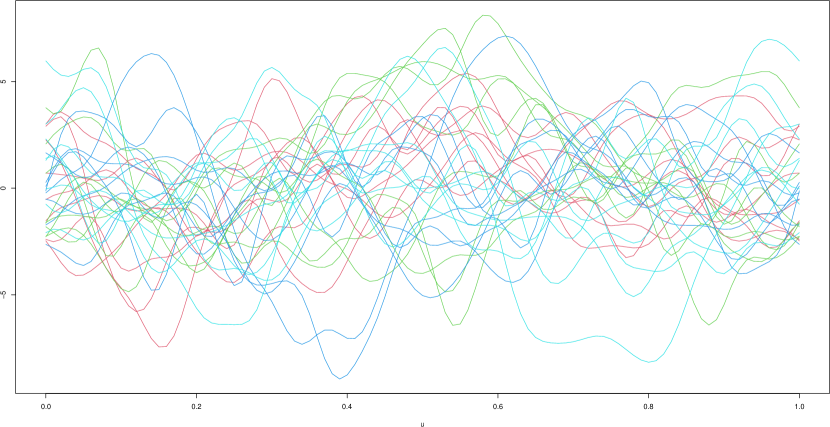
Figure 1: Examples of simulated functional data. The colours distinguish the four clusters.

First cluster
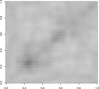
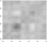
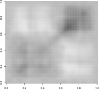
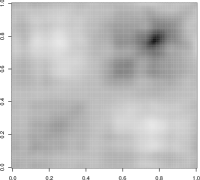
Second cluster
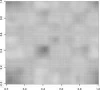
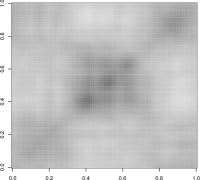
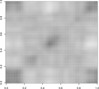
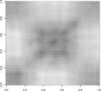
Third cluster
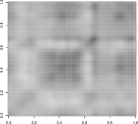
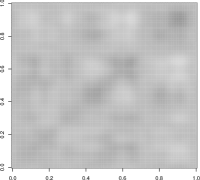
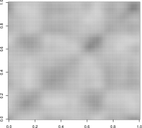
Fourth cluster

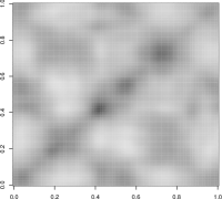
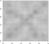
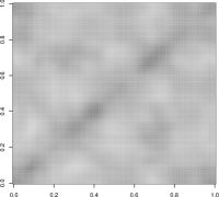
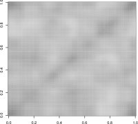
Figure 2: Examples of sample covariance operators of the simulated functional data.

For the two considered cases ($N=100$ and $N=10000$), Figure 3 displays the profiles of the trimmed average silhouette width obtained by applying the cluster algorithm for $K=2,\ldots,10$ to each of the simulated datasets. The profiles point to the correct number of clusters. In all the cases, the maximum was obtained exactly at $K=4$. Of course, in other scenarios, the performance of the suggested index can be inferior to that observed here.

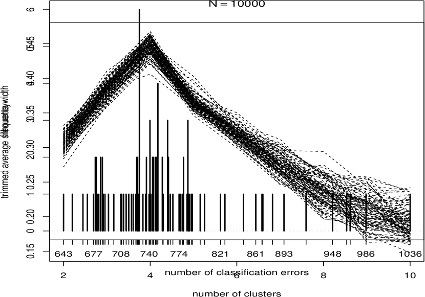
Figure 3: Synthetic data: The trimmed average silhouette width for $100$ simulated datasets with $N=100$ and $N=10000$ sample covariances. The true number of clusters is $K=4$.

In the remainder of this subsection, we focus on the quality of the classification results obtained for $K=4$. Figure 4 displays the empirical cumulative distribution functions of the error rates observed in the different simulated datasets when the “nearest allocation rule”

classify $\widehat{\Sigma}_{i}$ in the group whose prototype is $\overline{\Sigma}_{i_{a}}$ if $i_{a}=\arg\max_{j}\pi_{i,j}=\arg\min_{r}\Pi\bigl{(}\widehat{\Sigma}_{i},\overline{\Sigma}_{j}\bigr{)}$

is used. When $N=100$ and $N=10000$, the figure shows that the median of the classification errors is around $7\%$. In addition, observe that the error rates show little variability in the $N=10000$ case, which points to the limited effects of the additional randomization due to the selection of the $N_{reduced}=200$ covariances. Table 1 shows that the membership grades $\pi_{i,j}$ can capture the uncertainty of the classification, and so, in some sense, to predict the errors. In particular, the table shows the classification error rates of the “nearest allocation rule” subdivided for the levels of the credibility coefficients introduced in (10). Observe that the error rates are between $50\%$ and $60\%$ when the credibility of the allocation is low, that is, for about $5\%$ of the sample covariances for which $\max_{j}\pi_{i,j}$ was less than $0.5$. Then, the error rate decreases as the credibility of the allocation increases, reaching a value close to zero for about $70\%$ of the sample covariances for which $\max_{j}\pi_{i,j}>0.9$. It is also interesting to observe that the error rates are comparable, if not slightly lower, when $N=10000$ than when $N=100$. This finding confirms the limited impact of estimating the cluster barycenters using only part of the available sample covariances.

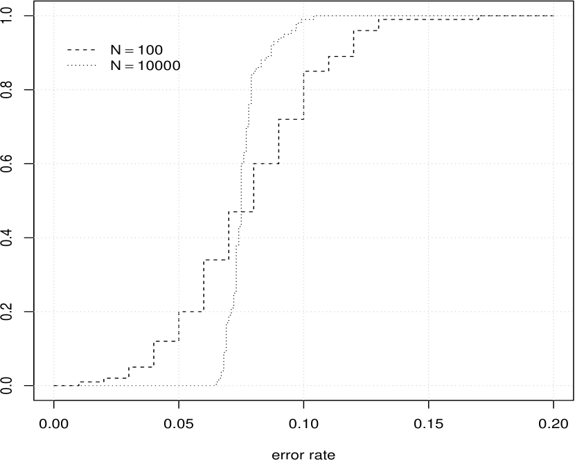
Figure 4: Synthetic data: cumulative distribution function of the error proportion of the “nearest allocation rule” in $100$ simulated datasets.

	Credibility of the “nearest allocation rule”
	$[0,0.5]$	$(0.5,0.6]$	$(0.6,0.7]$	$(0.7,0.8]$	$(0.8,0.9]$	$(0.9,1]$
	$N=100$
$\%$ covariances	0.047	0.049	0.051	0.060	0.100	0.693
Error rate	0.571	0.425	0.278	0.147	0.054	0.003
	$N=10000$
$\%$ covariances	0.048	0.047	0.050	0.063	0.104	0.686
Error rate	0.552	0.394	0.260	0.142	0.056	0.004

Table 1: Error rates of the “nearest allocation rule” for different levels of the credibility of the allocation. The credibility is given by $C_{i}=\max_{j=1,\ldots,K}\pi_{i,j}^{K}$.

4.2 Near-infrared gasoline spectra

In this subsection, we consider the gasoline near-infrared (NIR) spectra collected at an oil refinery and analyzed by Capizzi and Masarotto [7]. Production engineers collected 12 gasoline samples per day for 47 consecutive days. For each sample, the NIR absorbance is available for wavelengths from 900 to 1700 nm in intervals of 2 nm (thus, each spectrum is observed at 401 different wavelengths).

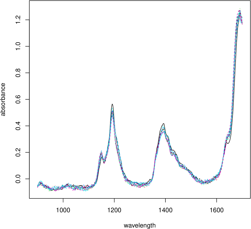
Figure 5: NIR spectra: the 564 observed curves.

Figure 5 shows the $12\times 47=564$ spectra. The data were gathered to understand if during the study there was day-to-day variability in the production conditions. However, the 12 samples collected each day were gathered several minutes apart, and therefore, it can be assumed that they were produced under the same set of conditions. Therefore, similar to what Capizzi and Masarotto [7] did, we assume that the data consist of $N=47$ samples (one for each day), each comprising $n=12$ curves. Capizzi and Masarotto [7] applied univariate distribution-free control charts separately to the first principal components (PC), and found an increase in the variability of the second, third, and fourth PCs during the days from 32 to 37. No differences in location in any PC, or in the variability of the other PCs, was identified. The instability in days 32–37 was then confirmed by the production engineers and attributed to a transitory malfunction of the automatic process adjustments that resulted in an increase in the variability of the product characteristics.

We applied our clustering algorithm (with $K=2,\ldots,5$) to the $47$ sample covariances estimated using the observations collected on the different days. Figure 6 shows the observed value of $TASW_{max}$ with an estimate of the null distribution under the hypothesis of no cluster obtained by $200$ random permutations of spectra centered using their day means. The results shown in the figure strongly suggest the presence of some clusters, that is, of some sort of day-to-day variation in the covariance structure. In particular, the $TASW$ profile, displayed in Figure 7, points to two clusters, and the corresponding weights $\pi_{i,1}$ and $\pi_{i,2}$ in Figure 7 single out the days from 32 to 37 from the others. An analysis of the two cluster barycenters $\overline{\Sigma}_{1}$ and $\overline{\Sigma}_{2}$ reveals differences in the absorbance standard deviations, essentially for each wavelength (see Figure 9). Thus, the use of the proposed approach allowed us to reach the conclusions reached by Capizzi and Masarotto [7] and confirmed by the plant managers about the presence of a transitory instability period.

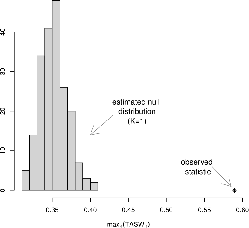
Figure 6: NIR spectra: observed $TASW_{max}$ statistic and an approximation of its null distribution under the hypothesis of no cluster computed using 200 permutations.

Figure 7: NIR spectra: trimmed average silhouette widths.

Figure 8: NIR spectra: weights $\pi_{i,j}$ of the solution obtained for $K=2$.

Figure 9: NIR spectra: diagonals of the covariance operators $\overline{\Sigma}_{1}$ and $\overline{\Sigma}_{2}$.

4.3 Phoneme data

In this subsection, we consider the dataset available at http://hastie.su.domains/ElemStatLearn/datasets, which consist of 4509 log-periodograms of length 256 computed from continuous speech frames of male speakers. The log-periodograms represent the pronunciation of the five phonemes: “aa”, “ao”, “dcl”, “iy”, and “sh”. With the aim of testing our clustering algorithm, we proceed as follows:

1. We randomly select, without replacement, $30$ subsamples each of size $40$ for each phoneme (thus, obtaining a total of $150$ subsamples).

2. We apply the proposed cluster algorithm to the corresponding $150$ sample covariances using $K=2,\ldots,10$ (and, of course, ignoring the known phoneme memberships).

To understand whether results were reproducible, the exercise was repeated four times. The code necessary to reproduce part of the first experiment is available in the supplementary material.

First experiment	Second experiment
Third experiment	Fourth experiment

Figure 10: Phoneme data: observed $TASW_{max}$ statistics and an approximation of its null distribution under the hypothesis of no cluster computed using 200 permutations.

Figure 10 shows the observed values of $TASW_{max}$ in the four replications, with an estimate of the null distribution under the hypothesis of no cluster obtained using $200$ random permutations of the (centered) log-periodograms selected during each exercise. As in the previous subsection, results strongly suggest the presence of a cluster structure in the data. The $TASW$ profiles, displayed in Figure 11, suggest $K=5$ in each of the four experiments. The visual representation, obtained by multidimensional scaling, of the

• “true” covariances of the five phonemes, that is, the covariances estimated using all the data for each phoneme, and

• the five cluster barycenters $\overline{\Sigma}_{1},\ldots,\overline{\Sigma}_{5}$

shows that the algorithm was consistently able to reconstruct the presence of the five phonemes.

First experiment	Second experiment
Third experiment	Fourth experiment

Figure 11: Phoneme data: trimmed average silhouette widths.

It is also interesting to observe that the partition matrix provides an idea of the degree of overlap between groups. For example, the cross-product of the matrix obtained for $K=5$ during the first experiment is

$$(P^{5})^{\prime}P^{5}=\begin{pmatrix}29.1\\ 0.1&22.5\\ 0.9&0.2&28.2\\ 0.1&1.8&0.1&25.0\\ 0.1&5.3&0.2&2.7&22.3\\ \end{pmatrix}.$$

A perusal of this matrix reveals that

• the first and third identified clusters are essentially isolated; indeed, the corresponding off-diagonal entries are quite small;

• the second and fifth clusters have a certain degree of overlap (the $(5,2)$ entry is the largest between the off-diagonal ones); there also exists a more limited overlap between these two clusters and the fourth cluster.

A look at the graph at the top left in Figure 12 makes clear the reasons for what we have just described: the second and fifth clusters correspond to the phonemes “ao” and “aa”, respectively. These two phonemes are, as expected, relatively hard to distinguish. The fourth cluster corresponds to the “iy” phoneme, which is closer to “ao” and “aa” than to the other two phonemes. Finally, the first and third clusters correspond to the phonemes “sh” and “dcl”, whose pronunciation is easier to distinguish. Analogous results were obtained for the other three replication of the exercise.

First experiment	Second experiment
Third experiment	Fourth experiment

Figure 12: Phoneme data: multidimensional scaling representation (principal coordinates analysis) based on the Wasserstein-Procrustes distance of the $5$ “true” phoneme covariances ($\Sigma_{\text{pnoneme}}$ with phoneme=“aa”, “ao”, “dcl”, “iy” and “sh”), and of the estimated cluster barycenters ($\overline{\Sigma}_{j}$ with $j=1,\ldots,5$).

5 Conclusions

We introduced a novel way to explore similarities among a group of functional covariance operators via a soft clustering mechanism based directly on the Wasserstein-Procrustes distance. The proposed framework is particularly useful in situations where there is no clean-cut cluster separation, and a certain degree of cluster overlapping could be envisaged. An attractive feature of the algorithm is that it allows to adjust for the expected degree of such overlapping, through the modulation of the average entropy level. Moreover, we contributed a novel cluster quality index, which we called the trimmed average silhouette width (TASW), which adapts the fast silhouette width considered by Van der Laan, Pollard and Bryan [31] to the covariance setting and “trims” it in a way that only clusters that are credibly far away (more than a given threshold) are considered. The TASW is shown empirically to behave well in simulations, and correctly estimate the proper number of clusters; however, different thresholds could be employed in the definition. We leave the details about the behaviour of different thresholds to future work. We also illustrate the use of the proposed methodology with an application to a gasoline near-infrared spectra dataset from Capizzi and Masarotto [7], and showed that the suggested approach allows us to reach the same conclusions as Capizzi and Masarotto [7] in a neat and simple way.

As a conclusive remark about future research, we would like to mention leveraging the geometric interpretation of the Wasserstein-Procrustes distance given in Masarotto, Panaretos and Zemel [21] that allows for the definition of other clustering algorithms, which perform partitioning on the tangent space of the nonlinear manifold inhabited by the covariance operators. Lifting the covariances to the tangent space makes it possible, and indeed interpretable, to shift the non-linear problem to a linear space, and for example, carry on traditional $k$-means based on the Hilbert–Schmidt distance. This intuition can be expanded further to develop hard and soft clustering methods.

Appendix A Proof of the proposition of Subsection 3.2

Point 1 of the proposition follows directly from (1). As for 2, observe that (5)–(7) can be easily obtained by introducing the Lagrange function

$${\cal L}=\sum_{i=1}^{N}\sum_{j=1}^{K}\pi_{i,j}d_{i,j}+\eta\left(\sum_{i=1}^{N}\sum_{j=1}^{K}\pi_{i,j}\log(\pi_{i,j})+NE\right)+\sum_{i=1}^{N}\lambda_{i}\left(\sum_{j=1}^{K}\pi_{i,j}-1\right),$$

where $d_{i,j}=\bigl{(}n_{i}-1\bigr{)}\Pi\bigl{(}\widehat{\Sigma}_{i},\overline{\Sigma}_{j}\bigr{)}$. In particular, equation (6) for the weights follows directly from the first-order conditions for $\lambda_{i}$ and $\pi_{ij}$

$$\dfrac{\partial{\cal L}}{\partial\pi_{i,j}} =d_{i,j}+\eta\bigl{(}\log(\pi_{i,j}\bigr{)}+1)+\lambda_{i}=0, (i=1,\ldots,N;j=1,\ldots,K),$$

$$\dfrac{\partial{\cal L}}{\partial\lambda_{i}} =\sum_{j=1}^{K}\pi_{i,j}-1=0, (i=1,\ldots,N).$$

Therefore, the constrained optimization problem becomes

$$\min_{\eta}\Phi(\eta)\text{ subject to }\Psi(\eta)=NE,$$

where $\Phi(\eta)=\sum_{i,j}\pi_{i,j}(\eta)d_{i,j}$ and $\Psi(\eta)=-\sum_{i,j}\pi_{i,j}(\eta)\log\pi_{i,j}(\eta)$. For simplicity, suppose that all the distances $d_{i,j}$ are distinct and greater than zero. This assumption will be true with probability one in applications (at least when the $X_{i,j}$’s are real). However, in any case, it is easy to adapt the following proof to the general case. Under the previous assumption, it is easy to show that

1. for every $i$ and $j$

   $$\lim_{\eta\rightarrow-\infty}\pi_{i,j}(\eta)=\lim_{\eta\rightarrow+\infty}\pi_{i,j}(\eta)=\dfrac{1}{K}.$$

   As a consequence,

   $$\lim_{\eta\rightarrow-\infty}\Phi(\eta)=\lim_{\eta\rightarrow+\infty}\Phi(\eta)=\Phi_{\infty}$$

   $$\lim_{\eta\rightarrow-\infty}\Psi(\eta)=\lim_{\eta\rightarrow+\infty}\Psi(\eta)=N\log K$$

   where

   $$\Phi_{\infty}=\dfrac{1}{K}\sum_{i,j}d_{i,j}.$$

2. for every $i$

   $$\lim_{\eta\rightarrow 0^{-}}\pi_{i,j}(\eta) =\begin{cases}0&\text{if }j\neq\arg\max_{r}d_{i,r}\\ 1&\text{if }j=\arg\max_{r}d_{i,r}\\ \end{cases}$$

   and

   $$\lim_{\eta\rightarrow 0^{+}}\pi_{i,j}(\eta) =\begin{cases}0&\text{if }j\neq\arg\min_{r}d_{i,r}\\ 1&\text{if }j=\arg\min_{r}d_{i,r}\\ \end{cases}.$$

   Thus,

   $$\lim_{\eta\rightarrow 0^{-}}\Phi(\eta)=\Phi_{0^{-}}\text{ and }\lim_{\eta\rightarrow 0^{+}}=\Phi_{0^{+}}$$

   with

   $$\Phi_{0^{-}}=\sum_{i}\max_{j}d_{i,j}\\ \text{ and }\Phi_{0^{+}}=\sum_{i}\min_{j}d_{i,j}.$$

   In addition,

   $$\lim_{\eta\rightarrow 0}\Psi(\eta)=0.$$

3. for every $\eta\neq 0$,

   $$\dfrac{d\Phi(\eta)}{d\eta}=\dfrac{V^{2}(\eta)}{\eta^{2}}\text{ and }\dfrac{d\Psi(\eta)}{d\eta}=\dfrac{V^{2}(\eta)}{\eta^{3}}$$

   where, defined $\overline{d}_{i}=\sum_{J}\pi_{i,j}d_{i,j}$,

   $$V^{2}(\eta)=\sum_{i,j}\pi_{i,j}\bigl{(}d_{i,j}-\overline{d}_{i}\bigr{)}^{2}.$$

When $0<E<\log K$, the previous properties show that $\Psi(\eta)$ monotonically decreases from $N\log K$ to $0$ when $\eta$ goes from $-\infty$ to $0$, and monotonically increases from $0$ to $N\log K$ when $\eta$ goes from $0$ to $+\infty$. Thus, the equation $\Psi(\eta)=NE$ has exactly two roots $-\infty<\eta^{-}<0<\eta^{+}<+\infty$. However, (a)–(c) also guarantee that $\Phi(\eta^{+})<\Phi_{\infty}<\Phi(\eta^{-})$, and, therefore, we only need to compute the positive root $\eta^{+}$. On the other hand, if $E=0$ (or $\log K$), the desired solution is given by the second degenerate distribution given in (b) (or by the uniform distribution given in (a)).

wasserstein.R:

R implementation of the proposed clustering method; the functions are documented inside the file.

phonemes.R:

R script that reproduces part of the phoneme example presented in Subsection 4.3.

References

- Agueh and Carlier [2011] {barticle}[author] \bauthor\bsnmAgueh, \bfnmMartial\binitsM. and \bauthor\bsnmCarlier, \bfnmGuillaume\binitsG. (\byear2011). \btitleBarycenters in the Wasserstein space. \bjournalSociety for Industrial and Applied Mathematics \bvolume43 \bpages904–924. \endbibitem
- Aneiros et al. [2022] {barticle}[author] \bauthor\bsnmAneiros, \bfnmGermán\binitsG., \bauthor\bsnmHorová, \bfnmIvana\binitsI., \bauthor\bsnmHušková, \bfnmMarie\binitsM. and \bauthor\bsnmVieu, \bfnmPhilippe\binitsP. (\byear2022). \btitleOn functional data analysis and related topics. \bjournalJournal of Multivariate Analysis \bvolume189 \bpages104861. \endbibitem
- Arbelaitz et al. [2013] {barticle}[author] \bauthor\bsnmArbelaitz, \bfnmOlatz\binitsO., \bauthor\bsnmGurrutxaga, \bfnmIbai\binitsI., \bauthor\bsnmMuguerza, \bfnmJavier\binitsJ., \bauthor\bsnmPérez, \bfnmJesús M.\binitsJ. M. and \bauthor\bsnmPerona, \bfnmIñigo\binitsI. (\byear2013). \btitleAn extensive comparative study of cluster validity indices. \bjournalPattern Recognition \bvolume46 \bpages243–256. \bdoi10.1016/j.patcog.2012.07.021 \endbibitem
- Batool and Hennig [2021] {barticle}[author] \bauthor\bsnmBatool, \bfnmFatima\binitsF. and \bauthor\bsnmHennig, \bfnmChristian\binitsC. (\byear2021). \btitleClustering with the average silhouette width. \bjournalComputational Statistics & Data Analysis \bvolume158 \bpages107190. \bdoi10.1016/j.csda.2021.107190 \endbibitem
- Boente, Rodriguez and Sued [2018] {barticle}[author] \bauthor\bsnmBoente, \bfnmGraciela\binitsG., \bauthor\bsnmRodriguez, \bfnmDaniela\binitsD. and \bauthor\bsnmSued, \bfnmMariela\binitsM. (\byear2018). \btitleTesting equality between several populations covariance operators. \bjournalAnnals of the Institute of Statistical Mathematics \bvolume70 \bpages919–950. \endbibitem
- Cabassi et al. [2017] {barticle}[author] \bauthor\bsnmCabassi, \bfnmAlessandra\binitsA., \bauthor\bsnmPigoli, \bfnmDavide\binitsD., \bauthor\bsnmSecchi, \bfnmPiercesare\binitsP. and \bauthor\bsnmCarter, \bfnmPatrick A\binitsP. A. (\byear2017). \btitlePermutation tests for the equality of covariance operators of functional data with applications to evolutionary biology. \bjournalElectronic Journal of Statistics \bvolume11 \bpages3815–3840. \endbibitem
- Capizzi and Masarotto [2018] {binproceedings}[author] \bauthor\bsnmCapizzi, \bfnmGiovanna\binitsG. and \bauthor\bsnmMasarotto, \bfnmGuido\binitsG. (\byear2018). \btitlePhase I distribution-free analysis with the R package dfphase1. In \bbooktitleFrontiers in Statistical Quality Control 12 (\beditor\bfnmSven\binitsS. \bsnmKnoth and \beditor\bfnmWolfgang\binitsW. \bsnmSchmid, eds.) \bpages3–19. \bpublisherSpringer International Publishing, \baddressCham. \endbibitem
- Chamroukhi and Nguyen [2019] {barticle}[author] \bauthor\bsnmChamroukhi, \bfnmFaicel\binitsF. and \bauthor\bsnmNguyen, \bfnmHien D\binitsH. D. (\byear2019). \btitleModel-based clustering and classification of functional data. \bjournalWiley Interdisciplinary Reviews: Data Mining and Knowledge Discovery \bvolume9 \bpagese1298. \endbibitem
- Fraley and Raftery [2002] {barticle}[author] \bauthor\bsnmFraley, \bfnmChris\binitsC. and \bauthor\bsnmRaftery, \bfnmAdrian E\binitsA. E. (\byear2002). \btitleModel-based clustering, discriminant analysis, and density estimation. \bjournalJournal of the American Statistical Association \bvolume97 \bpages611-631. \endbibitem
- Fréchet [1948] {barticle}[author] \bauthor\bsnmFréchet, \bfnmMaurice\binitsM. (\byear1948). \btitleLes éléments aléatoires de nature quelconque dans un espace distancié. \bjournalAnn. Inst. H. Poincaré \bvolume10 \bpages215–310. \endbibitem
- Fremdt et al. [2013] {barticle}[author] \bauthor\bsnmFremdt, \bfnmStefan\binitsS., \bauthor\bsnmSteinebach, \bfnmJosef G\binitsJ. G., \bauthor\bsnmHorváth, \bfnmLajos\binitsL. and \bauthor\bsnmKokoszka, \bfnmPiotr\binitsP. (\byear2013). \btitleTesting the equality of covariance operators in functional samples. \bjournalScandinavian Journal of Statistics \bvolume40 \bpages138–152. \endbibitem
- Ieva, Paganoni and Tarabelloni [2016] {barticle}[author] \bauthor\bsnmIeva, \bfnmFrancesca\binitsF., \bauthor\bsnmPaganoni, \bfnmAnna Maria\binitsA. M. and \bauthor\bsnmTarabelloni, \bfnmNicholas\binitsN. (\byear2016). \btitleCovariance-based clustering in multivariate and functional data analysis. \bjournalJournal of Machine Learning Research \bvolume17 \bpages1-21. \endbibitem
- Jacques and Preda [2014] {barticle}[author] \bauthor\bsnmJacques, \bfnmJulien\binitsJ. and \bauthor\bsnmPreda, \bfnmCristian\binitsC. (\byear2014). \btitleFunctional data clustering: a survey. \bjournalAdvances in Data Analysis and Classification \bvolume8 \bpages231–255. \endbibitem
- Jiao, Frostig and Ombao [2020] {barticle}[author] \bauthor\bsnmJiao, \bfnmShuhao\binitsS., \bauthor\bsnmFrostig, \bfnmRon D.\binitsR. D. and \bauthor\bsnmOmbao, \bfnmHernando\binitsH. (\byear2020). \btitleVariation pattern classification of functional data. \bjournalarXiv preprint https://arxiv.org/abs/2004.00855. \bdoi10.48550/ARXIV.2004.00855 \endbibitem
- Jiao, Frostig and Ombao [2022] {barticle}[author] \bauthor\bsnmJiao, \bfnmShuhao\binitsS., \bauthor\bsnmFrostig, \bfnmRon D.\binitsR. D. and \bauthor\bsnmOmbao, \bfnmHernando\binitsH. (\byear2022). \btitleBreak point detection for functional covariance. \bjournalScandinavian Journal of Statistics \bpagesEarly view article available at https://onlinelibrary.wiley.com/doi/10.1111/sjos.12589. \endbibitem
- Karcher [1977] {barticle}[author] \bauthor\bsnmKarcher, \bfnmHermann\binitsH. (\byear1977). \btitleRiemannian center of mass and mollifier smoothing. \bjournalCommunications on pure and applied mathematics \bvolume30 \bpages509–541. \endbibitem
- Kashlak, Aston and Nickl [2019] {barticle}[author] \bauthor\bsnmKashlak, \bfnmAdam B\binitsA. B., \bauthor\bsnmAston, \bfnmJohn AD\binitsJ. A. and \bauthor\bsnmNickl, \bfnmRichard\binitsR. (\byear2019). \btitleInference on covariance operators via concentration inequalities: k-sample tests, classification, and clustering via Rademacher complexities. \bjournalSankhya A \bvolume81 \bpages214–243. \endbibitem
- Kaufman and Rousseeuw [2009] {bbook}[author] \bauthor\bsnmKaufman, \bfnmLeonard\binitsL. and \bauthor\bsnmRousseeuw, \bfnmPeter J\binitsP. J. (\byear2009). \btitleFinding groups in data: an introduction to cluster analysis. \bpublisherJohn Wiley & Sons. \endbibitem
- Kraus and Panaretos [2012] {barticle}[author] \bauthor\bsnmKraus, \bfnmDavid\binitsD. and \bauthor\bsnmPanaretos, \bfnmVictor M\binitsV. M. (\byear2012). \btitleDispersion operators and resistant second-order functional data analysis. \bjournalBiometrika \bvolume99 \bpages813–832. \endbibitem
- Lee et al. [2015] {barticle}[author] \bauthor\bsnmLee, \bfnmHaesung\binitsH., \bauthor\bsnmAhn, \bfnmHyun-Jung\binitsH.-J., \bauthor\bsnmKim, \bfnmKwang-Rae\binitsK.-R., \bauthor\bsnmKim, \bfnmPeter T\binitsP. T. and \bauthor\bsnmKoo, \bfnmJa-Yong\binitsJ.-Y. (\byear2015). \btitleGeodesic clustering for covariance matrices. \bjournalCommunications for Statistical Applications and Methods \bvolume22 \bpages321–331. \endbibitem