Satellite Content and Halo Mass of Galaxy Clusters: Comparison between Red-Sequence and Halo-based Optical Cluster Finders

Abstract

Cluster cosmology depends critically on how optical clusters are selected from imaging surveys. We compare the conditional luminosity function (CLF) and weak lensing halo masses between two different cluster samples at fixed richness, detected within the same volume ($0.1{<}z{<}0.34$) using the red-sequence and halo-based methods. After calibrating our CLF deprojection method against mock galaxy samples, we measure the 3D CLFs by cross-correlating clusters with SDSS photometric galaxies. As expected, the CLFs of red-sequence and halo-based finders exhibit redder and bluer populations, respectively. The red-sequence clusters have a flat distribution of red galaxies at the faint end, while the halo-based clusters host a decreasing faint red and a boosted blue population at the bright end. By comparing subsamples of clusters that have a match between the two catalogues to those without matches, we discover that the CLF shape is mainly caused by the different cluster centroiding. However, the average weak lensing halo mass between the matched and non-matched clusters are consistent with each other in either cluster sample for halos with $\lambda>30$ ($M_{h}^{\mathrm{WL}}{>}1.5\times 10^{14}h^{-1}M_{\odot}$). Since the colour preferences of the two cluster finders are almost orthogonal, such a consistency indicates that the scatter in the mass-richness relation of either cluster sample is close to random. Therefore, while the choice of how optical clusters are identified impacts the satellite content, our result suggests that it should not introduce strong systematic biases in cluster cosmology, except for the $\lambda<30$ regime.

1 Introduction

Galaxy clusters are one of the most sensitive probes of dark energy and cosmic growth (see section 6 of Weinberg et al., 2013, for a comprehensive review), but cluster cosmology in the optical is currently in a state of minor crisis. The most recent cosmological constraints using galaxy clusters (e.g., Abbott et al., 2020; Costanzi et al., 2021; Park et al., 2021) favored lower $\Omega_{m}$ and higher $\sigma_{8}$ compared against the constraints inferred from the cosmic microwave background (Planck Collaboration et al., 2020), large-scale structures traced by galaxies (Alam et al., 2017; Beutler et al., 2011; Abbott et al., 2018), and clusters detected with Sunyaev-Zeldovich (Bocquet et al., 2019) and X-ray (Mantz et al., 2015; Chiu et al., 2022) observations. To resolve this discrepancy, much work has been done to determine which systematic uncertainties may be responsible. For instance, projection effects are believed to boost the richness (i.e., the number of galaxies above some luminosity threshold) and the large-scale weak lensing (WL) signal of optical clusters (Zu et al., 2017; Busch & White, 2017), and therefore potentially bias cosmological constraints (e.g., Abbott et al., 2020; Sunayama et al., 2020; Myles et al., 2021; Wu et al., 2022; Zeng et al., 2022).

Although the projection effects in optical cluster cosmology are problematic, they may mask a larger overall issue. The methods currently used to optically identify galaxy clusters are imperfect and have existing biases that must be taken into account. For the past twenty years, the two primary methods used to identify optical clusters from photometric surveys are the red sequence-based cluster finder, which uses overdensities of “red and dead” galaxies on the sky to select cluster candidates (e.g., Gladders & Yee, 2000, 2005; Miller et al., 2005; Rykoff et al., 2012, 2014, 2016) and the halo-based method (Yang et al., 2005, 2007, 2021), which instead relies on the overdensities of all galaxies above some magnitude threshold, including the blue galaxies that are often excluded by the red sequence (also see Wen et al., 2012; Tinker, 2021; Zou et al., 2021; Tinker, 2022). Although these methods greatly differ, both have been used to successfully identify large samples of cluster candidates with reasonably high completeness and purity.

Both methods of identifying galaxy clusters unavoidably have their own preferences for the satellite content. Identifying clusters using the red sequence works well at $z{<}1$ where clusters have long been observationally dominated by strong red sequences (Gladders & Yee, 2000). Under the assumption that the red sequence forms as a result of halo quenching (i.e., the probability of a galaxy being quiescent depends only on halo mass (Birnboim & Dekel, 2003; Zu & Mandelbaum, 2015)) red sequence-based cluster finders should be efficient at sifting out the most massive systems without introducing any biases due to the colour selection. However, red-sequence clusters may be more strongly impacted by halo assembly bias (e.g., Gao et al., 2005; Gao & White, 2007; Jing et al., 2007; Dalal et al., 2008), as these overdensities of quiescent galaxies may be older clusters with higher concentrations that more efficiently formed at early times (Zu et al., 2021, 2022). Additionally, this method does not account for the blue galaxies that observations have found exist abundantly within the cluster environment, which may impact the observational properties of the cluster.

Initially developed with the spectroscopic galaxies in mind (Yang et al., 2005, 2007), the halo-based method has been shown to work across a wide redshift range and have a high completeness of clusters even when applied to imaging data (Yang et al., 2021). This method evaluates the membership probabilities for all galaxies regardless of colour, and relies on the total luminosity of all member galaxies as a proxy of halo mass, which may result in weighting blue galaxies more favorably than the red ones. The primary bias for this method results from photometric-redshift estimates, which are poorer for blue galaxies, leading to contamination in the membership due to stronger projection effects. In the current work, we exploit the fact that the detection preferences associated with the red-sequence and halo-based finders are roughly orthogonal, and investigate the differences not just between the two cluster catalogues, but also between clusters that are co-detected by both finders and those detected only once.

One primary statistical measurement used to characterize the galaxy content within clusters is the conditional luminosity function (CLF; Yang et al., 2003), defined as the luminosity function of all the cluster member galaxies at fixed halo mass. Traditionally, the CLFs of photometric clusters are measured by directly counting the number of member galaxy candidates identified by the cluster finder, sometimes weighted by the inferred membership probabilities (e.g., To et al., 2020). However, such a direct method is incapable of recovering the true underlying CLFs of the haloes, primarily due to biases in the colour selection and background contamination caused by projection effects (Zu et al., 2017). Instead of using the membership provided by cluster catalogues, one could take advantage of the excellent photometric redshifts of clusters, and measure the CLFs by cross-correlating clusters with galaxies from imaging data (Hansen et al., 2009; Lan et al., 2016; Meng et al., 2022). This approach accounts for the CLF contribution of all galaxies regardless of colour, and the contamination from interloper galaxies from distant, uncorrelated structures can be statistically removed by subtracting the measurement around random points on the sky. Moreover, the contribution of galaxies that are outside the 3D radius of the cluster but in a physically correlated structure along the line-of-sight (e.g., in the filaments that connect to the cluster) can be modelled theoretically (Lan et al., 2016). As a result, instead of measuring the CLF properties of individual clusters, this cross-correlation or “stacking” approach measures the parameters associated with ensembles of clusters that are stacked together based on a given richness. In this work, we follow this stacking methodology to explore the different CLFs of clusters detected by red-sequence and halo-based cluster finders.

Robust measurements of CLFs depend critically on the correct identification of central galaxies, which is unfortunately challenging to achieve for current optical cluster finders using just the imaging data (e.g., Johnston et al., 2007; George et al., 2012; Hollowood et al., 2019). Miscentring would result in a partial overlap between the measurement aperture and the true cluster region, leading to an underestimation of the CLF amplitudes and, more problematic, biases in the shape of the CLFs due to the clumpiness of satellite distribution within clusters. This issue can be statistically remedied in cluster weak lensing studies by introducing a miscentring kernel that can be calibrated against the X-ray centres (Zhang et al., 2019a) and convolved with a theoretical dark matter density profile (Navarro et al., 1997). However, the correct underlying CLFs cannot be reconstructed with the same procedure, primarily because the true CLF model is unknown (especially at the faint end). In this work, for the first time we investigate the impact of miscentring on the measured shape of the CLF, by examining the CLFs of the same clusters but centred differently by the two cluster finders.

Discrepancies in the galaxy content between clusters detected with different cluster finders do not necessarily introduce significant biases in cosmological analyses. For a volume-complete cluster sample above some true halo mass $M_{h}$, the red sequence-based and halo-based cluster finders may both detect all the clusters but assign them richnesses with differing amounts of logarithmic scatter at fixed halo mass. In the ideal scenario, such a scatter in the mass-richness relation could be purely statistical in nature, and thus can be self-calibrated when constraining cosmology with clusters (Rozo et al., 2010; Tinker et al., 2012; Zu et al., 2014). However, if the cluster finder preferentially assigns higher richnesses to haloes with a particular CLF, such as having a higher red fraction due to older formation time, or higher blue fraction due to stronger projection effects within dense environments, the scatter is no longer random and would systematically bias the constraint on cosmological parameters. In this work, we take advantage of the orthogonal CLF preferences between the red-sequence and halo-based finders, and divide each catalogue into two subsamples based on whether the clusters are also detected by the other cluster finder. Therefore, by examining whether there exists any significant discrepancy in the average halo mass measured from weak lensing between the two subsamples, we can better understand the nature of the scatter in the mass-richness relation for different cluster finders.

The structure of the paper is as follows. In Section 2, we describe the photometric galaxy catalogue and cluster samples selected for this analysis. In Section 3, we describe how the CLFs are measured in both samples and compare the galaxy content revealed by their CLFs. In Section 4 we describe the cluster weak lensing measurements and compare the weak lensing halo masses between the matched vs. non-matched clusters within each sample. We conclude the paper and look to the future in Section 5. Throughout this analysis, we assume a flat $\Lambda$CDM characterized by Planck Collaboration et al. (2020) cosmology with $\Omega_{M}$=0.315 and $h$=0.674. Additionally, we note that unless explicitly stated, we are using $\log\,M_{h}$ for the logarithm with base 10 of halo mass in unit of $h^{-1}M_{\odot}$, defined by the halo radius within which the mean halo density is $\Delta{=}200$ times the mean density of the Universe. Finally, all distances measured are co-moving distances in units of $h^{-1}\mathrm{Mpc}$.

2 Data

2.1 The SDSS Photometric Galaxy Sample

In this analysis, we measure the CLF by statistically counting the galaxies from a photometric catalogue constructed using Sloan Digital Sky Survey Data Release 16 (SDSS DR16; York et al., 2000; Ahumada et al., 2020). We select all galaxies with clean photometry (CLEAN=1) with an SDSS r-band Galactic extinction-corrected model-magnitude greater than 21 (modelmag_r$-$extinction_r<21.0) for completeness. In total, this yields a sample of about 47 million galaxies within a sky coverage of approximately 8500 deg².

For measuring the CLF contribution from any given cluster at redshift, $z$, we estimate the absolute magnitude M_r for each galaxy assuming it is at the redshift of that cluster as $M_{r}{=}m_{r}{-}\mathrm{DM}(z)$, where $m_{r}$ is the apparent magnitude after being corrected for Galactic extinction and DM($z$) is the distance modulus at the redshift of the cluster. Interloper galaxies that are not physically associated or correlated with the cluster, hence assigned the wrong redshift, will be statistically removed by the background subtraction (as discussed in Section 3.3).

We note that because our goal for this analysis is a comparison of the CLF measured in clusters identified in the Rykoff et al. and Yang et al. catalogues within a relatively narrow redshift range ($0.1{<}z{<}0.34$), we choose not to account for the K-correction, which systematically shifts the CLFs by the same amount for both measurements. Moreover, the K-correction to $z=0.1$ is of the order of $\sim$0.1 magnitudes across our redshift range and given our average bin size (0.4 magnitudes) when measuring the CLF would only have a minimal impact on our presented results.

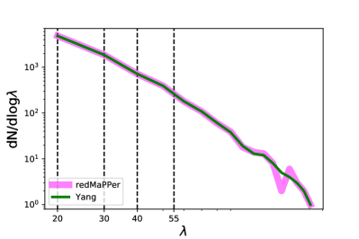
Figure 1: The richness distributions of the Yang (thin green curve) and redMaPPer (thick magenta curve) samples. The richness estimates of Yang clusters are measured by counting the total number of member galaxies brighter than $M_{r}{=}{-}20.4$ and enclosed within an $1h^{-1}\mathrm{Mpc}$ aperture, and then abundance-matched to the richness distribution of redMaPPer clusters, hence the consistency between the two curves. Vertical dashed lines indicate the edges of the four richness bins adopted in our analysis.

2.2 Red Sequenced-based Cluster Sample: redMaPPer

The red sequenced-based cluster catalogue we employ is the SDSS redMaPPer v6.3 cluster catalogue (Rykoff et al., 2014) derived by applying a red-sequence-based photometric cluster finding algorithm to the SDSS DR8 imaging (Aihara et al., 2011). Briefly, redMaPPer iteratively self-trains a model of red-sequence galaxies calibrated by an input spectroscopic galaxy sample, and then attempts to grow a galaxy cluster centred on every photometric galaxy. Once a galaxy cluster has been identified by the matched-filters, the algorithm iteratively solves for a photometric redshift based on the calibrated red-sequence model, and recentres the clusters about the best candidates for central galaxies.

Therefore, each redMaPPer cluster is a conglomerate of red-sequence galaxies on the sky, with each galaxy assigned a membership probability $p_{\mathrm{mem}}$ and a probability of being the central $p_{\mathrm{cen}}$. For each cluster, the richness $\lambda_{\mathrm{RM}}$ is computed by summing the $p_{\mathrm{mem}}$ of all member galaxy candidates, and roughly corresponds to the number of red-sequence satellite galaxies brighter than $0.2\,L_{*}$ within an aperture of ${\sim}1\,h^{-1}\mathrm{Mpc}$ (with a weak dependence on $\lambda_{\mathrm{RM}}$). At $\lambda_{\mathrm{RM}}{\geq}20$, the SDSS redMaPPer cluster catalogue is approximately volume-complete up to $z{\simeq}0.34$ (Groenewald et al., 2017), with cluster photometric redshift uncertainties as small as $\delta(z)=0.006/(1+z)$ (Rykoff et al., 2014; Rozo et al., 2015).

We use the $\lambda{\geq}20$ sample between $z{=}0.1$ and $0.34$. For this analysis, our initial sample of redMaPPer clusters consists of the 9226 clusters between the redshift range $0.10<z<0.34$. For each cluster we identify the most likely central galaxy candidate provided by redMaPPer and treat its location as the centre for the CLF measurement.

2.3 Halo-based Cluster Sample of Yang et al. (2021)

The halo-based clusters used in this analysis are detected by the Yang et al. (2021) cluster finder (hereafter referred to as the Yang clusters). This cluster finder is an extension of the spectroscopic group finder previously developed by Yang et al. (2005, 2007) and has been updated to incorporate both photometric and spectroscopic information. The photometric data used to construct the Yang et al. (2021) catalogue comes from the DESI Legacy Imaging Survey DR9 (Dey et al., 2019), which covers the redshift range $0.0<z\leq 1.0$.

We briefly summarise the halo-based methodology used in the Yang cluster finder below and refer interested readers to Yang et al. (2021) for the technical details. The halo-based algorithm attempts to build groups or clusters centred on every galaxy within the legacy imaging data by assigning initial membership to galaxies using a friends-of-friends approach assuming some small linking length (Yang et al., 2007). Using the total luminosity within these initial overdensities, the mass-to-light ratio of each cluster is determined via abundance matching, which allows each tentative cluster to be assigned a halo mass. Cluster membership is then determined assuming the galaxy distribution follows the same phase-space distribution as the dark matter particles. This requirement selects all member galaxies above a background level within $R_{180}$ from the luminosity-weighted cluster centre. This process is then repeated iteratively (3-4 times) until the mass-to-light ratios converge. Using mock galaxy samples, Yang et al. (2021) demonstrated that this adaptive halo-based algorithm can reliably detect systems with mass above a few ${\times}10^{13}h^{-1}M_{\odot}$ with a purity higher than 90%.

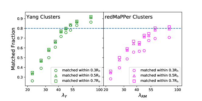
Figure 2: The matched fraction as a function of richness for the Yang (left panel) and redMaPPer (right panel) cluster samples, using three different search radii of 0.3$R_{h}$ (circles), 0.5$R_{h}$ (triangles), and 0.7$R_{h}$ (squares). We adopt the cross-matching results using the 0.7$R_{h}$ search radius as our fiducial split between matched vs. non-matched clusters in the paper.

The Yang catalogue provides an abundance-matched halo mass, $M_{180}^{L_{\mathrm{tot}}}$, defined with $\Delta{=}180$ instead of $200$ and based on the total luminosity of galaxies in the cluster (with DESI z-band apparent magnitude ${z_{\rm DESI}}$<21.0 within $R_{180}$). Yang et al. (2021) showed that the scatter about the $M_{180}^{L_{\mathrm{tot}}}$-$M_{h}$ relation is about 0.2 dex above $10^{14}h^{-1}M_{\odot}$, similar to that in redMaPPer. For centring, instead of computing $p_{\mathrm{cen}}$ as done in redMaPPer, the Yang catalogue adopts the luminosity-weighted centre as the fiducial centre of a cluster. For this analysis, we do not cover the entire redshift range of the Yang catalogue, but instead use data only from the redshift range over which redMaPPer is complete as well as only those clusters with $\log M_{180}^{L_{\mathrm{tot}}}{\geq}14.0$. These cuts limit the Yang sample to 29014 clusters. We also note that although this catalogue was developed using the DESI imaging, we measure the CLF for Yang clusters using the same SDSS photometric data as for redMaPPer.

2.4 redMaPPer and Yang Clusters within the Same Volume

The purpose of our CLF analysis is to compare the galaxy populations within haloes identified by either redMaPPer or the Yang cluster finder. However, these two cluster catalogues are identified using different galaxy surveys and cover different spatial and redshift regions. To account for this, we only select clusters in the overlapping footprint between the two samples and within the redshift range $0.1<z<0.34$ where both samples are reasonably complete at the high mass end. The DESI legacy imaging footprint is larger than the region covered by SDSS, so much of the data removed is from the Yang catalogue. In total, the number of redMaPPer clusters was reduced to 8770, a reduction of less than 5%. In contrast, the number of Yang clusters was reduced to 15063, a reduction of 48.1%. Moreover, to accurately compute the covering fraction of any regions on the sky, we require that each cluster be within the SDSS BOSS spectroscopic footprint, for which convenient window and mask polygon files are available. Removing clusters outside the BOSS window (minus the bright star masks) function slightly reduces the number of available clusters in each footprint. The redMaPPer cluster sample then consists of 8300 clusters and the Yang sample consists of 14155 clusters, a reduction of 5.4% and 6.0%, respectively.

To facilitate the comparison between these two cluster samples, we need to account for the difference in the aperture sizes adopted by the two cluster finders when defining their respective halo mass proxy. In particular, redMaPPer provides a richness ($\lambda_{\mathrm{RM}}$) measured within roughly 1$h^{-1}\mathrm{Mpc}$, while the $M_{180}^{L_{\mathrm{tot}}}$ of Yang clusters are estimated within $R_{180}$, which is usually larger than 1$h^{-1}\mathrm{Mpc}$. Therefore, for each Yang cluster, we redefine a new richness $\lambda^{\mathrm{new}}_{\mathrm{Y}}$ by measuring the total number of member galaxies (with equal weights) with SDSS r-band absolute magnitudes $M_{r}{<}{-}20.4$, enclosed within a fixed $1h^{-1}\mathrm{Mpc}$ aperture centred on the luminosity-weighted centre. The member galaxies are directly adopted from the Yang membership catalogue, which is roughly volume-complete above $M_{r}{>}-20.4$ between $0.1{<}z{<}0.34$.

To further bring the two richness measurements ($\lambda^{\mathrm{new}}_{\mathrm{Y}}$ vs. $\lambda_{\mathrm{RM}}$) to the same scale, we perform a standard abundance matching (assuming zero scatter) to ensure that the richness distribution of the top 8300 Yang clusters (ranked by $\lambda^{\mathrm{new}}_{\mathrm{Y}}$) is the same as the $\lambda_{\mathrm{RM}}$ distribution of the 8300 redMaPPer clusters. After abundance matching, we reassign a richness value $\lambda_{\mathrm{Y}}$ to each of the top 8300 Yang clusters, and adopt $\lambda_{\mathrm{Y}}$ for the Yang clusters for the remainder of the paper. Figure 1 shows the richness distributions of the redMaPPer (thick magenta curves) and Yang (thin green curves) clusters within the same volume, using the $\lambda_{\mathrm{RM}}$ and $\lambda_{\mathrm{Y}}$ estimates, respectively. Going forward, unless otherwise noted we will refer to both richnesses as $\lambda$.

Using the two abundance matched samples, we follow the approach used in Lan et al. (2016) and only select clusters into our final analysis samples with a covering fraction within 1$h^{-1}\mathrm{Mpc}$ from the cluster centre higher than 95%. This cut is needed to remove clusters located at the edges of the survey as well as those near regions that are masked by bright foreground stars. This criteria reduces the number of clusters in our final sample to 7582 for redMaPPer and 7562 for Yang, reductions of 8.7% and 8.9%, respectively.

Finally, for the CLF and weak lensing analyses we divide each cluster sample into four subsamples based on $\lambda$, indicated by the vertical dashed lines in Figure 1 — the four richness bins are $\lambda=[20,\,30]$, $[30,\,40]$, $[40,\,55]$, and $[55,\,200]$, respectively.

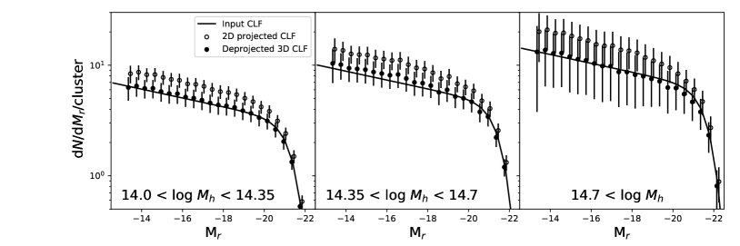
Figure 3: Validation of the CLF deprojection method using mock photometric galaxies in three different halo mass bins. In each panel, the black solid line is the input CLF from Yang et al. (2008), open circles are the 2D projected CLF measured from the stacking method, and filled circles are the 3D deprojected CLF from the 2D results, using the magnitude-dependent correction factor at each halo mass bin $f_{\mathrm{corr}}(M_{r})$. There is excellent agreement between the deprojected 3D CLF and the input CLF.

2.4.1 Cross-Matching Cluster Samples

As discussed in Section 1, we also investigate the properties between the clusters that are co-detected by both cluster finders and those detected in one but not in the other. To cross-match between the two catalogues, for a cluster from one catalogue, we identify from the other catalogue any cluster detected within some projected 2D radial aperture and with a redshift within 3$\sigma_{z}$ as a match, where $\sigma_{z}$ is the uncertainty on the photometric redshift estimate. For redMaPPer this is $\delta(z)/(1+z)$ and $\approx$0.006 at $z=0.1$ and $\approx$0.015 at $z=0.3$ (Rykoff et al., 2014; Rozo et al., 2015); For Yang clusters this is $\sigma_{z}\approx 0.008$ (Yang et al., 2021). For this cross-matching, we only use the two final samples, so a cluster classified as “non-matched” might have a matched counterpart with $\lambda<20$ in the other cluster catalogue. Were we to use the entire samples (down to much lower $\lambda$), as well as extend out to arbitrarily larger radii, the matched fraction would increase significantly, thereby making the comparison less useful.

As shown in Figure 2, we use three different search radii, 0.3R_h, 0.5R_h and 0.7R_h. For the sake of simplicity we use $R_{h}$ that corresponds to the original apertures adopted by the cluster finders. We see that for the most massive clusters ($\lambda{\simeq}55$), the matched fraction is greater than 80% for a search radius greater than 0.5R_h. Unsurprisingly, the matched fraction decreases with decreasing richness, as the matches are increasingly more likely to be found in the $\lambda<20$ systems. Besides, the completeness and purity of both cluster catalogues also drop rapidly with richness. We note that a more complete analysis of the comparison between the clusters and groups identified by redMaPPer and the Yang cluster finder is needed, but beyond the scope of this analysis. For the analysis in this paper, we adopt 0.7R_h as the fiducial search radius for our matched vs. non-matched split.

3 The Conditional Luminosity Functions

3.1 Stacked 2D CLF Measurement

To compare the satellite populations within clusters from both catalogues, we measure the CLF for clusters within each $\lambda$ bin. The standard approach (e.g., Hansen et al., 2009; Lan et al., 2016) is to separate the central and satellite components of the CLFs. However, because the Yang clusters are not centered on the central galaxy and the central is included when measuring the CLF within 1$h^{-1}\mathrm{Mpc}$ of the luminosity weighted center, we include the central galaxy component in the measurements of all CLFs in this analysis. Despite this inclusion of centrals in the CLFs, we only focus on the magnitude range dominated by the satellite galaxies and refer to the member galaxies at those magnitudes simply as “satellites” during our CLF comparison. In an upcoming analysis, we plan to build on this work and use the central galaxy to investigate the impact of the magnitude gap, a tracer of BCG hierarchical growth (Golden-Marx & Miller, 2018), on the CLF.

Unlike some previous analyses (e.g., To et al., 2020), we do not directly use either the redMaPPer or the Yang membership candidates to construct the CLF (though we present that direct result as well). Instead, we closely follow the stacking procedures of Lan et al. (2016) to measure the CLF of both cluster catalogues using the SDSS photometric galaxies. Using the centroid positions identified in those catalogues, for each galaxy cluster, we identify all galaxies within a projected distance of 1$h^{-1}\mathrm{Mpc}$. We use a constant radial aperture to mitigate the impact of uncertainties in the halo mass estimates. We then convert their apparent magnitudes into absolute magnitudes assuming the cluster redshift. However, as previously noted because this is a photometric measurement, we must account for contamination from interloper galaxies. For each cluster, we assign the redshift and halo mass to ten random points within the survey footprint and use the same 1$h^{-1}\mathrm{Mpc}$ aperture to determine the background contribution. By subtracting off the background from the measurement centred on the cluster centre, we obtain the 2D CLF measurement for each individual cluster.

We next employ the BOSS window function (with bright stars masked out) to estimate the covering fraction of each cluster region. More specifically, we determine what fraction of the sky within a 1$h^{-1}\mathrm{Mpc}$ aperture is not masked as a result of bright stars or edge effects. The covering fractions are generally high as our final analysis sample includes only those clusters with covering fraction greater than 95%. We multiply the measured CLF by the inverse of this fraction to correct for masking. Additionally, when stacking the measurements, we use the limiting magnitude of the SDSS observations ($m_{r}{=}21$) to calculate the absolute magnitude limit for each cluster and correct for this difference across our redshift range $0.1{<}z{<}0.34$. We then calculate the stacked 2D CLF by measuring the mean 2D CLF within 1$h^{-1}\mathrm{Mpc}$ of the cluster centre (with the mean random background contribution subtracted) for each of the four richness bins described in Section 2.4.

At this point, we are left with a 2D CLF, which is representative of the average galaxy population projected within a 1$h^{-1}\mathrm{Mpc}$ 2D aperture about the cluster centre. However, our goal is to estimate the 3D isotropic CLF within a 1$h^{-1}\mathrm{Mpc}$ radius, for which we need to further remove the CLF contribution from galaxies in the correlated structures but physically outside the 1$h^{-1}\mathrm{Mpc}$ radius.

3.2 Deprojecting 2D CLF to 3D: Mock Test using N-body Simulation

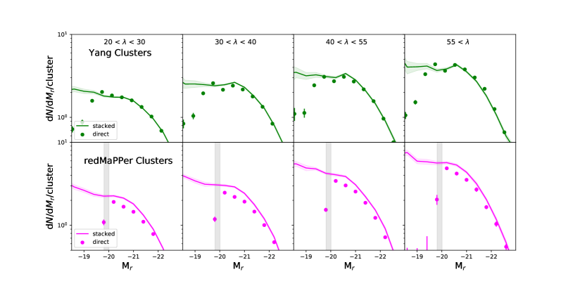
Figure 4: For four bins in $\lambda$, we compare the CLF measured directly from the membership catalogues (circles with errorbars) to those measured from cross-correlating with the photometric galaxies (curves with uncertainty bands) in both the Yang (top row) and redMaPPer (bottom row) catalogues. In the lower panels, we denote $0.2L_{*}$ as the gray band.

We compute the correction factor to deproject the CLF measurements from 2D to 3D by following the approach outlined in Lan et al. (2016). Although such a deprojection approach has been applied to real data by Lan et al. (2016), we verify our capability of accurately measuring the average CLF per cluster within a 3D radius using a sample of simulated clusters and a mock catalogue of photometric galaxies. In particular, we determine whether any additional calibrations are needed to accurately remove the contribution from correlated structures to the CLF when deprojecting the 2D measurements to 3D.

Using the ELUCID N-body constrained cosmological simulation (Wang et al., 2016), we construct the mock photometric galaxy catalogue by populating dark matter haloes according to the halo mass-dependent CLF parameters measured by Yang et al. (2008). For a continuous coverage of the ELUCID halo mass function with galaxies down to $m_{r}{=}21$, we interpolate the CLF parameters across the three most massive bins of Yang et al. (2008) and extrapolate the CLFs of Yang et al. (2008) to fainter magnitudes assuming fixed faint-end slopes. We further assume the galaxy distribution follows an isotropic NFW profile inside the dark matter haloes with the same concentration and velocity dispersion as the dark matter particles. Following Salcedo et al. (2022), we populate the halos within the SDSS main sample volume inside the ELUCID constrained simulation.

Following the approach outlined in the Appendix B2 of Lan et al. (2016), we calculate a correction factor $f_{\mathrm{corr}}$ to account for the discrepancy that exists between the CLF projected within a 2D aperture and that enclosed within a 3D halo radius, which results from galaxies associated with the correlated structure outside the clusters. We briefly describe the deprojection method below and refer interested readers to Lan et al. (2016) for the analytic derivations. To determine this correction factor at any given magnitude for each halo mass/richness bin, $f_{\mathrm{corr}}(M_{r})$, we measure the normalized surface number density of galaxies at a given magnitude between 0.1R₂₀₀ and 2.5R₂₀₀ and fit the power-law slope, $\gamma$, to this profile. We then use equation B7 from Lan et al. (2016) to convert the power-law slope $\gamma$ to the correction factor $f_{\mathrm{corr}}$. We note that this process differs from Lan et al. (2016) in that we adopt a magnitude-dependent $\gamma$ to remove the contribution from the correlated structure instead of measuring the median value of $\gamma$ within each richness bin.

As shown in Figure 3, the 2D CLF overpredicts the number of galaxies associated with each cluster. However, after applying the correction factors to the 2D CLF, our deprojected 3D CLF is in excellent agreement with the theoretical input from Yang et al. (2008). Thus, the magnitude-dependent correction factors are needed to accurately reproduce the input CLF. Therefore, in our observational analysis, we measure the surface density profile out to 2.5R₂₀₀ at fixed $M_{r}$ for each cluster and measure the correction factor as a function of $M_{r}$ for clusters of each richness bin.

3.3 Stacked 3D CLFs: Comparison with Direct CLFs

After testing the stacking and deprojection method with mock galaxy samples, we are now ready to apply the method to the redMaPPer and Yang cluster samples using the SDSS photometric catalogue. We apply the correction factor $f_{\mathrm{corr}}(M_{r}|\lambda)$ to each 2D CLF to remove the effect of galaxies that are outside of our 1$h^{-1}\mathrm{Mpc}$ radius when measured in 3D, thereby converting our previously measured 2D CLFs to the deprojected 3D CLFs.

Although both the redMaPPer and Yang cluster catalogues provide membership catalogues to identify the galaxies associated with each cluster, the uncertainties associated with the membership probabilities are generally large, with significant biases due to the redshift uncertainties and projection effects (Zu et al., 2017). Therefore, CLFs constructed directly from those membership catalogues (hereafter referred to as “direct” CLFs) are expected to be incomplete. Figure 4 presents the results of the direct CLF when measured within 1$h^{-1}\mathrm{Mpc}$ for each membership catalogue, compared to the 3D CLF measured from the stacking method (band). For the direct CLFs of Yang clusters, we apply a constant shift of 0.07 magnitudes to convert the DESI magnitudes of the member galaxies to SDSS r-band magnitudes $M_{r}$. We note that redMaPPer also provides a membership probability $p_{\mathrm{mem}}$, which we use in our estimate of the direct CLF.

As shown in Figure 4, we find very similar trends between the direct and stacked CLFs for both the Yang (top row) and redMaPPer (bottom row) clusters at the bright end ($M_{r}{<}{-}21.5$), indicating that both cluster finders are highly effective in identifying the bright member galaxies. At the faint end, we note that redMaPPer uses a limiting magnitude of $0.2L_{*}$ (gray vertical bands) to determine its membership catalogue. As a result, it is unsurprising that we see the redMaPPer direct CLF (filled circles) drop off beyond that limit. Meanwhile, the Yang catalogue imposes an apparent magnitude cut on the membership galaxies, so we do not observe a steep drop-off in the direct measurement like what is seen in redMaPPer, and their direct and stacked CLFs are in reasonable agreement until $M_{r}{\sim}{-}19.5$. Interestingly, the direct CLFs of both Yang and redMaPPer exhibit a modest deficit compared to their respective stacked CLFs at ${-}20{>}M_{r}{>}{-}21$, suggesting that both cluster finders are relatively conservative in assigning memberships to galaxies with intermediate luminosities between sub-$L_{*}$ and $L_{*}$. However, we note that the deficit should be caused by the incompleteness of different types of galaxies, (relatively redder galaxies in Yang and bluer galaxies in redMaPPer).

3.4 CLF Comparison between the Yang and redMaPPer Clusters

3.4.1 CLF Amplitudes

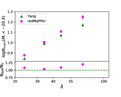
Figure 5: Comparison between the total number of member galaxies $N_{\mathrm{mem}}$ between the Yang (green triangles) and redMaPPer (magenta circles) clusters in four different richness bins. The satellite numbers are computed from integrating the stacked CLFs above $M_{r}{=}{-}20.4$. The lower panel shows the ratio of the number of members in the redMaPPer clusters divided by that in the Yang clusters.

We compute the total number of member galaxies brighter than $M_{r}{=}-20.4$, $N_{\mathrm{mem}}$, by integrating the stacked CLFs of both cluster samples at fixed $\lambda$ (as shown in Figure 4) above ${-}20.4$. Figure 5 compares the $N_{\mathrm{mem}}$ between the Yang (green triangles) and redMaPPer (magenta circles) clusters in the four richness bins, with the ratios $N_{\mathrm{RM}}/N_{\mathrm{Y}}$ (circles) shown in the bottom panel. The number of member galaxies at the lower richness end ($\lambda$$\leq$55) are in good agreement (within $10\%$). In contrast, at the higher richness end the redMaPPer clusters contain $\sim$20% more member galaxies. By using a fixed $1h^{-1}\mathrm{Mpc}$ aperture, we eliminate the impact of halo definitions. Therefore, the discrepancy is likely driven by the combination of different centring and scatters in the mass-richness relation between the two catalogues. In particular, it is likely that 1) the centrals identified by redMaPPer are located in denser regions than the luminosity-weighted centre from the Yang catalogue; and 2) the new $\lambda_{\mathrm{Y}}$ richness that we redefined for the Yang catalogue has a slightly larger scatter (at fixed halo mass) than $\lambda_{\mathrm{RM}}$ and $M_{180}^{L_{\mathrm{tot}}}$ (i.e., the original halo mass proxy of the Yang catalogue) at the high mass end, thereby finding intrinsically lower mass clusters at the same $\lambda$. However, as discussed further in Section 4, our cluster weak lensing analysis suggests that the relatively larger scatter in our new richness $\lambda_{\mathrm{Y}}$ is likely the more dominant cause, which is expected because $\lambda_{\mathrm{Y}}$ is not optimized for minimising the scatter in the mass-richness relation. Additionally, we note that when using the BCGs identified by Yang (not shown in this analysis), this $N_{\mathrm{mem}}$ discrepancy is enlarged, suggesting that the luminosity-weighted centres are indeed better choices for the CLF measurement.

3.4.2 Dependence of the CLF Shape on Galaxy Colour and Cluster Finders

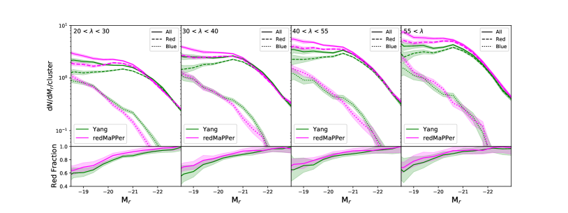
Figure 6: Comparison of the CLF shapes between the Yang (green) and redMaPPer (magenta) clusters in four richness bins. In each upper panel, the total CLF (solid curves) is decomposed into the contributions from red (dashed curves) and blue (dotted curves) galaxies. The lower panels show the red fractions as functions of the absolute r-band magnitude.

We now focus on the shapes of the stacked CLFs to compare the galaxy content at different absolute magnitudes between the redMaPPer and Yang clusters. Additionally, to examine the colour difference in the galaxy content, we split our photometric galaxies by colour to measure the stacked CLFs of the red and blue satellites separately. Unlike Lan et al. (2016), who used $u{-}r$ colour, or Meng et al. (2022), who used $g{-}z$ colour, we use the redshift-dependent redMaPPer red-sequence defined in $g{-}r$ to identify all red galaxies across the redshift range of interest. This approach also accounts for the shallow slope of the red sequence on the colour-magnitude diagram at any given redshift. We then identify galaxies with $g{-}r$ colours 2$\sigma$ below the red sequence as blue and all other galaxies as red.

Figure 6 compares the CLFs between the redMaPPer and Yang clusters using the two overall samples (i.e., regardless of whether a cluster in one sample has a matched counterpart in the other sample). At the bright end ($M_{r}<-20.4$), where the massive red galaxies dominate the CLFs, the shapes are in excellent agreement. However, the faint-end slopes of the overall CLF (solid curves) differ, with $\alpha_{\mathrm{Yang}}{\simeq}{-}0.90$ (green) and $\alpha_{\mathrm{RM}}{\simeq}{-}1.1$ (magenta). This discrepancy appears to be driven by the lower luminosity red galaxies (dashed curves), where redMaPPer clusters exhibit a relatively constant population, compared to the slightly decreasing population in Yang clusters. Meanwhile, we detect a boost in the population of blue galaxies in the Yang clusters at $M_{r}{<}{-}21$ compared to the redMaPPer clusters, and the amplitude of the boost declines with increasing richness, exhibiting little difference between the two blue CLFs in the highest-$\lambda$ bin. Both discrepancies in the red and blue CLFs are consistent with our expectation that the colour preferences of the red-sequence and halo-based cluster finders are largely orthogonal. The bottom panels show the red fractions as functions of $M_{r}$, further demonstrating that the redMaPPer clusters are systematically redder than the Yang clusters.

Naively, one might expect the shape discrepancy between the redMaPPer and Yang CLFs shown in Figure 6 to be caused mainly by the mismatched clusters (i.e., clusters detected in one catalogue but not in the other). However, from Figure 2 we know that the mismatched fraction rapidly decreases as a function of $\lambda$, but that the shape discrepancies in the overall and red CLFs shown in Figure 6 are consistent across the four richness bins. Therefore, while the mismatched clusters are likely the culprit for the discrepancy in the blue CLFs (the $\lambda$-dependent boost at $M_{r}{<}{-}21$), the discrepancy in the red CLFs (hence overall CLFs) is mainly due to the different centring algorithms between the two cluster finders. To test this hypothesis, we disentangle the effect of centring from that of mismatching by splitting the Yang clusters at each $\lambda$ bin into two subsamples, one with matched counterparts in the redMaPPer sample based on our fiducial cross-matching criteria (hereafter referred to as “matched”), and the other one without (“non-matched”). In Figure 7, we show the stacked CLFs of the matched clusters using both the original Yang luminosity-weighted centres (solid curves) and the highest-$p_{\mathrm{cen}}$ galaxies of their matched counterparts in redMaPPer (dashed curves), as well as the stacked CLF of the non-matched clusters using their original Yang centres (dotted curves). Similar to Figure 6, we decompose each CLF into the contributions from red (red curves) and blue (blue curves) galaxies, and show the red fractions in the bottom panels.

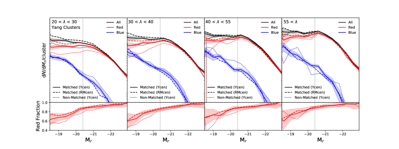
Figure 7: Comparison of the CLF shapes between the Yang clusters that have matched counterparts in redMaPPer using luminosity-weighted centers (solid curves with uncertainty bands), the same matched clusters using redMaPPer centrals as centers (dashed curves), and the Yang clusters with no matched counterparts in redMaPPer (dotted curves) in four different richness bins. In each upper panel, the overall CLF of each subsample (black) is decomposed into contributions from the red (red) and blue (blue) satellite galaxies. The lower panels show the red fractions as functions of r-band absolute magnitude.

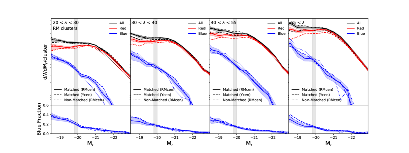
Figure 8: Similar to Figure 7, but for redMaPPer clusters. The lower panels show the blue fractions as functions of r-band absolute magnitude.

By comparing the CLFs of the matched clusters measured with different centres, we find that the shape discrepancy induced by switching centres closely mimics that between the Yang and redMaPPer CLFs seen in Figure 6. The flat (decreasing) population of all (red) faint satellites observed around Yang centres (solid black/red curves) becomes increasing (flat) at the faint end when switching to the redMaPPer centrals (dashed curves). Therefore, we conclude that these shape differences between the overall (as well as red) CLFs measured for the two cluster catalogues are primarily caused by the different centring algorithms. The redMaPPer algorithm tends to identify the location of the most densely populated pocket of red galaxies as the centre of a cluster, while the luminosity-weighted centre found by Yang likely sits more closely to the geometric centre of a larger cluster region but may miss the true centre (defined by the minimum of the potential) by a large margin in morphologically-disturbed systems. As a result, neither centring algorithm works perfectly in all scenarios, and it is thus more plausible that the true CLF of a correctly-centred cluster sample (e.g., by X-ray observations) is closer to the average of the two versions. We plan to test this hypothesis by measuring the CLF for clusters with well measured X-ray centres in the future.

For the Yang clusters with no matched counterparts in redMaPPer (dotted blue curves), their blue galaxy CLFs are similar to those of the matched clusters (solid blue curves) in shape, but with a slightly larger amplitude at the bright end. However, for non-matched clusters, the red galaxy CLFs (dotted red curves) are significantly lower than the red galaxy CLFs of the matched clusters (solid red curves), by an amount ranging from 20% in the highest richness bin to a factor of two in the lowest richness bin. Consequently, the red fraction of the non-matched clusters is systematically lower than that of the matched clusters in all richness bins (bottom panels). Since those non-matched clusters are significantly less dominated by the red galaxies than the matched clusters, it is unsurprising that the redMaPPer algorithm does not detect them as clusters with $\lambda{>}20$. Meanwhile, the Yang cluster finder detects progressively more systems with bluer satellite population than redMaPPer, especially in low-richness systems.

We perform a similar test using the redMaPPer sample by splitting the redMaPPer clusters into matched vs. non-matched subsamples based on the existence of matched counterparts in the Yang sample. The result is shown in Figure 8. Likewise, the shape discrepancy persists in the matched clusters (solid black curves), but promptly disappear after we adopt the same centres for these clusters (dashed black curves). The increasing (relatively flat) population of all (red) faint galaxies when centered on the redMaPPer central transforms into the relatively flat (slightly decreasing) population of all (red) low-luminosity galaxies when centred on the Yang luminosity weighted center. Interestingly, the red galaxy CLFs of the matched vs. non-matched clusters are consistent across all richness bins, as the redMaPPer algorithm regards them as indistinguishable by counting the red galaxies. However, the blue CLFs of the non-matched clusters (dotted blue curves) are much lower than those of the matched clusters (solid blue curves) in the two low-richness bins, while the two sets of blue CLFs are consistent in the two high-richness bins, mirroring the trend seen for the Yang sample in Figure 7. As a result, the bottom panels show that the blue fraction of the non-matched clusters (dotted blue curves) is generally lower than that of the matched clusters (solid blue curves).

To summarise the results from Figures 7 and  8, the shape of the overall CLFs are primarily sensitive to the centroiding of clusters. In particular, the faint-end slope could exhibit an increasing or a decreasing trend, depending on whether the cluster centres are located within a dense clump of red galaxies or a luminosity-weighted centre averaged over a large spread of both red and blue galaxies. In addition, some of the discrepancies in the CLF shapes are caused by the orthogonal colour preferences between the two cluster finders, resulting in the non-detection of the extremely red-dominated clusters by Yang and the relatively blue clusters by redMaPPer, respectively.

3.5 CLF Parameters and Comparison to Previous Results

Since the introduction of the Schechter Function (Schechter, 1976), the observed CLF has been characterised by its amplitude ($\phi^{*})$, characteristic luminosity ($M^{*}$), and faint-end slope ($\alpha$), all information which provides insight into the physical processes that characterise galaxy formation and evolution. To measure the three parameters associated with our CLF for each of the samples shown in Figures 6,  7, and  8, we fit our measured CLF to a function of the form

$$\phi(M_{r})=\frac{\ln(10)}{2.5}\phi^{*}10^{0.4(M^{*}-M_{r})(\alpha+1)}\exp[{-10^{0.4(M^{*}-M_{r})}}],$$ (1)

using a standard Bayesian inference method using the Markov Chain Monte Carlo (MCMC) ensemble sampler PyMC. The results are given in Table 1 along with the redMaPPer results when the central is not included. In addition, the CLF parameters for the (non-) matched subsamples of the Yang and redMaPPer clusters are provided in the Appendix in Tables 3 and  4, respectively.

Table 1: Best-fitting parameters of the CLFs in Figure 6 .

bin	M∗	$\alpha$	$\phi^{*}$
All galaxies of Yang clusters
1	-22.02 $\pm$ 0.04	-0.99 $\pm$ 0.02	2.44 $\pm$ 0.09
2	-21.65 $\pm$ 0.04	-0.83 $\pm$ 0.03	4.60 $\pm$ 0.16
3	-21.64 $\pm$ 0.05	-0.88 $\pm$ 0.03	5.40 $\pm$ 0.24
4	-21.65 $\pm$ 0.06	-0.89 $\pm$ 0.04	6.66 $\pm$ 0.35
Red galaxies of Yang clusters
1	-21.93 $\pm$ 0.03	-0.83 $\pm$ 0.02	2.48 $\pm$ 0.07
2	-21.61 $\pm$ 0.04	-0.70 $\pm$ 0.03	4.41 $\pm$ 0.14
3	-21.61 $\pm$ 0.05	-0.77 $\pm$ 0.03	5.16 $\pm$ 0.22
4	-21.59 $\pm$ 0.06	-0.78 $\pm$ 0.04	6.65 $\pm$ 0.34
Blue galaxies of Yang clusters
1	-21.63 $\pm$ 0.14	-1.47 $\pm$ 0.05	0.29 $\pm$ 0.05
2	-21.29 $\pm$ 0.17	-1.30 $\pm$ 0.09	0.55 $\pm$ 0.12
3	-21.34 $\pm$ 0.20	-1.30 $\pm$ 0.11	0.58 $\pm$ 0.15
4	-21.37 $\pm$ 0.27	-1.43 $\pm$ 0.13	0.52 $\pm$ 0.18
All galaxies of redMaPPer clusters
1	-22.13 $\pm$ 0.04	-1.15 $\pm$ 0.02	2.14 $\pm$ 0.11
2	-21.96 $\pm$ 0.05	-1.10 $\pm$ 0.02	3.35 $\pm$ 0.16
3	-21.84 $\pm$ 0.05	-1.11 $\pm$ 0.03	4.63 $\pm$ 0.26
4	-21.78 $\pm$ 0.06	-1.06 $\pm$ 0.03	6.83 $\pm$ 0.44
Red galaxies of redMaPPer clusters
1	-22.03 $\pm$ 0.04	-1.01 $\pm$ 0.02	2.34 $\pm$ 0.09
2	-21.82 $\pm$ 0.04	-0.95 $\pm$ 0.02	3.72 $\pm$ 0.16
3	-21.75 $\pm$ 0.05	-0.99 $\pm$ 0.03	4.89 $\pm$ 0.24
4	-21.71 $\pm$ 0.05	-0.95 $\pm$ 0.03	7.05 $\pm$ 0.40
Blue galaxies of redMaPPer clusters
1	-21.20 $\pm$ 0.17	-1.57 $\pm$ 0.07	0.32 $\pm$ 0.07
2	-21.46 $\pm$ 0.24	-1.57 $\pm$ 0.09	0.32 $\pm$ 0.10
3	-21.43 $\pm$ 0.29	-1.61 $\pm$ 0.10	0.38 $\pm$ 0.16
4	-21.55 $\pm$ 0.30	-1.67 $\pm$ 0.10	0.36 $\pm$ 0.15
All galaxies of redMaPPer clusters - no BCG
1	-21.50 $\pm$ 0.03	-0.94 $\pm$ 0.02	3.64 $\pm$ 0.14
2	-21.59 $\pm$ 0.04	-0.98 $\pm$ 0.02	4.54 $\pm$ 0.19
3	-21.58 $\pm$ 0.04	-1.00 $\pm$ 0.03	5.83 $\pm$ 0.28
4	-21.59 $\pm$ 0.05	-0.99 $\pm$ 0.03	8.01 $\pm$ 0.48
Red galaxies of redMaPPer clusters - no BCG
1	-21.38 $\pm$ 0.03	-0.75 $\pm$ 0.02	3.83 $\pm$ 0.11
2	-21.46 $\pm$ 0.04	-0.80 $\pm$ 0.02	4.90 $\pm$ 0.17
3	-21.50 $\pm$ 0.04	-0.89 $\pm$ 0.03	6.00 $\pm$ 0.25
4	-21.51 $\pm$ 0.05	-0.87 $\pm$ 0.03	8.32 $\pm$ 0.44
Blue galaxies of redMaPPer clusters - no BCG
1	-21.19 $\pm$ 0.17	-1.57 $\pm$ 0.07	0.32 $\pm$ 0.08
2	-21.46 $\pm$ 0.24	-1.57 $\pm$ 0.09	0.32 $\pm$ 0.10
3	-21.43 $\pm$ 0.29	-1.61 $\pm$ 0.10	0.38 $\pm$ 0.16
4	-21.55 $\pm$ 0.29	-1.68 $\pm$ 0.10	0.36 $\pm$ 0.15

The primary takeaway from measuring the parameters, given in Table 1, is that only $\phi^{*}$ depends on $\lambda$, in agreement with the results from Hansen et al. (2009). However, the comparison between the parameters measured for the redMaPPer and Yang clusters is more insightful. As given in Table 1, the underlying parameters within the CLF slightly differ, as suggested by Figure 6. We find that the $M^{*}$ for redMaPPer and Yang clusters are largely consistent, which reflects the location of the bright-end turn-over in Figure 6. Moreover, as shown in Figure 6, we see that the faint-end slope, $\alpha$ for the redMaPPer catalogue is slightly steeper, for both red, blue, and overall galaxies. Lastly, as previously mentioned, we unsurprisingly find that the amplitude $\phi^{*}$ is generally larger for the redMaPPer sample, in agreement with the results from Figure 5.

Since the galaxy cluster CLF is well studied, there are many results we can compare our stacked measurements to. However, these parameters are mildly covariant, so the inclusion of the central galaxy, which impacts the measurement of M^∗ also impacts $\alpha$ and $\phi$. Based on the inclusion of the central, we do not compare our measured M^∗ to previous results. However, we also present the redMaPPer results without the central galaxy to make a comparison to the $\alpha$ measurements from Hansen et al. (2009) and Zhang et al. (2019b).

One of the best comparison samples is from Zhang et al. (2019b), who measured the CLFs of clusters identified by redMaPPer in the Dark Energy Survey (DES) using the DES Science Verification data (Rykoff et al., 2016). Although this analysis covers both a larger range in halo mass and higher redshift, we find strong agreement between our $\alpha$ value for red galaxies when the BCG is excluded with their measurement, $\alpha{\simeq}{-}0.7-0.8$, for DES- redMaPPer selected clusters in our redshift range. Of note, Zhang et al. (2019b) also detect a similar trend in $\alpha$, such that the value becomes slightly steeper with richness.

We also compare our results to Hansen et al. (2009), which cover a similar redshift and halo mass range, but instead use the MaxBCG catalogue (Koester et al., 2007). We note that Hansen et al. (2009) measure the CLF within R₂₀₀ as opposed to a 1$h^{-1}\mathrm{Mpc}$ aperture; however, as shown in their Figure 3, their average aperture size is comparable to ours. Another difference is that Hansen et al. (2009) fix $\alpha$ for the blue galaxies, while we allow it to be a free parameter. Given our use of a similar aperture, it is unsurprising that we measure similar values $\phi^{*}$ for both the red and blue samples and the overall sample. Additionally, the $\alpha$ value for red galaxies ($\alpha{\simeq}{-}0.7$) and overall galaxy sample ($\alpha{\simeq}{-}0.9$) show general agreement with our results excluding the BCG, though our values are $\sim$0.1 steeper. For both of our samples, the blue galaxy $\alpha$ is much steeper than what Hansen et al. (2009) assume, $\alpha_{blue}{=}{-}1.0$. Some of these discrepancies may result from the difference in cluster finding algorithm and how red and blue galaxies are defined. Hansen et al. (2009) uses a fixed bimodal definition based on $g{-}r$ colours, while we use the redMaPPer defined red sequence which is redshift dependent.

Although measured for lower redshift galaxy clusters, we compare our results to those presented in Lan et al. (2016) ($0.01<z<0.05$) and Meng et al. (2022) ($0.01<z<0.08$), which use clusters identified in the Yang et al. (2007) spectroscopic group catalogue. The primary differences between our measurement approaches are the different apertures within which we measure the CLF (1$h^{-1}\mathrm{Mpc}$ vs R₂₀₀), how we identify red and blue galaxies, and our inclusion of the central galaxy. However, given that we both use the halo-based cluster finder, this is a relevant comparison. We note that we only compare our results to the bright portion of the measurements presented in Lan et al. (2016) and Meng et al. (2022), because we do not observe the magnitude range fainter than $M_{r}{=}{-}18$) due to the higher redshift nature of our cluster samples.

For the total sample of galaxies, our measurements for $\alpha$ are in agreement with the results from both Lan et al. (2016) and Meng et al. (2022). For the red galaxies, our values of $\alpha$ are in agreement at the lowest-$\lambda$ end, while at the high-richness end, our $\alpha$ is shallower by 0.15-2 than both Lan et al. (2016) and Meng et al. (2022). For blue galaxies, we find that our measurements for $\alpha$ are in agreement with the values presented in Lan et al. (2016) and Meng et al. (2022) for the entire $\lambda$ range. We note that the difference between our measurements and those from Lan et al. (2016) and Meng et al. (2022) is primarily due to the different performances of the photometric and spectroscopic halo-based cluster finders as well as our inclusion of the central galaxy.

In addition to the CLF parameters, we also compare our measured red fractions to those from Hansen et al. (2009) and Meng et al. (2022). Hansen et al. (2009) measure a red fraction within the entire cluster of $\sim$80% for galaxy clusters, in strong agreement with the results we find for both the redMaPPer and Yang samples. In a more direct comparison, Meng et al. (2022) find that the red fraction increases slightly with $\lambda$ and that it also increases from 60% to 100% with $M_{r}$ over the range $-18>M_{r}>-23$, which is in excellent agreement with our measurement shown in Figure 6.

In Lan et al. (2016), one of their primary conclusions is that the CLF can be characterised by a faint-end slope that steepens at $M_{r}=-18.0$. This same faint-end slope was similarly detected by Tinker et al. (2021) and Meng et al. (2022) for CLF samples measured at low redshifts ($z<0.08$). Although the higher average redshift of our sample prevents us from directly making this measurement, we address this comparison by extrapolating our faint-end behaviors to fainter magnitudes. In particular, Lan et al. (2016) note that the increase in the faint-end slope is driven predominately by the red galaxies, where $\alpha=-1.8$. Moreover, both Lan et al. (2016) and Meng et al. (2022) find that the fraction of red galaxies greatly increases in the magnitude range $-12<M_{r}<-16$, and thus results in that faint end slope. However, it is worth noting that this trend was identified using groups and clusters identified in the Yang et al. (2007) spectroscopic group catalogue, using the luminosity-weighted centres. Interestingly, Figure 6 suggests we may see that the faint-end population starts to modestly rise at $M_{r}{=}{-}19$ for some richness bins. However, even though we do not analyse the faintest $M_{r}$ range of interest, we find that the CLF shape is sensitive to the centring algorithm used and we expect this conclusion to hold at fainter magnitudes. Therefore, while Lan et al. (2016) and Meng et al. (2022) suggest that this steeper faint-end slope is a result of the different formation processes behind red and blue galaxies in the cluster environment, our results suggest that this effect may be impacted by the choice of cluster finder, particularly the way the centres of the galaxy clusters are identified.

To summarise the results from our stacked CLF comparison, we confirm the expectation that the redMaPPer cluster finder generally detects clusters with a higher fraction of red galaxies and vice versa for the Yang finder. However, the shape discrepancy between the CLFs of the two cluster samples is, somewhat unexpectedly, mainly due to the difference in cluster centring between the two finders. For a cluster cosmology analysis, however, this is very encouraging news because cluster miscentring can be robustly calibrated using X-ray data (Zhang et al., 2019a) and accurately modelled out in the cluster weak lensing analysis when measuring halo mass (e.g., Zu et al., 2021; Wang et al., 2022), the key quantity for cluster cosmology.

4 Weak Lensing Halo Mass of Clusters

4.1 Weak Lensing of Matched vs. Non-Matched Clusters

After examining the discrepancy in the galaxy content between the two cluster samples, we now explore whether a significant systematic uncertainty exists as a result of any cluster detection bias associated with the galaxy content preferred by each finder. As mentioned in Section 1, it is plausible that the detection bias associated with a particular cluster finder would drive the otherwise random scatter in the mass-richness relation to be systematic, sometimes with strong non-Gaussian tails. For example, if a cluster finder preferentially assigns higher richnesses to haloes with a higher red fraction due to an older formation time, while misdetecting young haloes with higher blue fraction but the same halo mass. The scatter in the mass-richness relation would have a systematic contribution, so that the halo mass distribution at fixed richness would include a long tail into the low-mass regime. By the same token, another cluster finder could assign higher richnesses to systems with an excess number of blue galaxies projected within the 2D aperture due to the larger photo-z errors of blue galaxies, thereby producing a similar long tail at the low-mass end. Unfortunately, it is observationally challenging to ascertain the existence of such a systematic component in the scatter, as the underlying halo mass distribution of the clusters is unknown.

Table 2: Parameter descriptions and priors for WL halo mass inference.

Parameter	Description	Prior
$\log M_{h}^{\mathrm{WL}}$	Log-halo mass	$\mathcal{U}$(13.0,16.0)
c	Halo concentration	$\mathcal{N}$(5,1.52)
$f_{\rm off,RM}$	redMaPPer offset fraction	$\mathcal{N}$(0.30,0.042)
$\sigma_{\rm off,RM}$	redMaPPer characteristic offset	$\mathcal{N}$(0.18,0.022)
$f_{\rm off,Y}$	Yang offset fraction	$\mathcal{U}$(0.0, 1.0)
$\sigma_{\rm off,Y}$	Yang characteristic offset	$\mathcal{U}$(0.0,1.0)

$\mathcal{N}(a,b)$ refers to a Normal distribution with mean and variance of a and b and $\mathcal{U}(a,b)$ refers to a uniform distribution with upper and lower limits a and b.

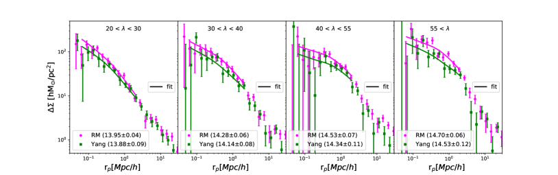
Figure 9: The $\Delta\Sigma$ profiles of the Yang (green squares with errorbars) and redMaPPer (magenta circles with errorbars) clusters in four different richness bins. Solid green and magenta lines are the best-fitting model curves for the Yang and redMaPPer clusters, respectively.

However, by taking advantage of the two cluster samples within the same volume detected by complementary approaches, we can circumvent the issue by exploring whether a significant discrepancy exists in the average halo masses estimated from weak lensing ($M_{h}^{\mathrm{WL}}$), in particular between the matched and the non-matched clusters at fixed $\lambda$ of each cluster catalogue. The rationale is as follows. Assuming cluster catalogues $\mathcal{A}$ and $\mathcal{B}$ have detection biases that are roughly orthogonal, at fixed $\lambda$ of catalogue $\mathcal{A}$, clusters that have matched counterparts in $\mathcal{B}$ are likely the systems that are least affected by the detection bias of $\mathcal{A}$, while the $\mathcal{A}$ clusters that do not have any matches in $\mathcal{B}$ are potentially the ones that are intrinsically low-mass systems but promoted above the richness/detection threshold of $\mathcal{A}$. Therefore, if we observe a significant discrepancy in the weak lensing halo mass of the matched vs. non-matched clusters from $\mathcal{A}$, this would suggest the existence of a strong systematic component in the scatter, which would then lead to severe bias in the cluster cosmology analysis.

We follow a similar approach to estimate $M_{h}^{\mathrm{WL}}$ as what is described in depth in Zu et al. (2021) and use the same shear catalogue as in Wang et al. (2022). Therefore, here we describe the data used for our measurements and how we fit the $\Delta\Sigma$, excess surface density profile. A more detailed description of our cluster weak lensing formalism is provided in the Appendix. The weak gravitational lensing signal is measured using the weak lensing shear catalogue derived from the Dark Energy Camera Legacy Survey (DECaLS) DR8 (Dey et al., 2019), which is part of the DESI Legacy Imaging Survey. For this analysis, our source galaxy photometry and photometric redshifts come from Zou et al. (2019). These redshifts are supplemented with the photometric redshifts estimates from (Zhou et al., 2021). For each richness bin, the shear catalogues are constructed from the DECaLS DR8 data using the Fourier_Quad method (Zhang et al., 2015, 2019c; Zhang et al., 2022).

4.2 Bayesian Modelling of Cluster Weak Lensing on Small Scales

In this analysis, we use a Bayesian framework to infer the weak lensing halo masses directly from the $\Delta\Sigma$ profiles, following the same method as outlined in Zu et al. (2021). Since our goal is to measure the halo mass $M_{h}^{\mathrm{WL}}$, we only use the $\Delta\Sigma$ profiles measured at radii below the transition scale between the so-called one-halo and two-halo terms, which occurs at $\sim$2$h^{-1}\mathrm{Mpc}$ (Zu et al., 2014).

For each of the four $\lambda$ bins, we have four parameters that we are fitting for the $\Delta\Sigma$ profile, including the halo mass $M_{h}^{\mathrm{WL}}$, halo concentration $c$, fraction of miscentred clusters with offset from the true halo centre $f_{\rm off}$, and the characteristic offset of miscentred clusters $\sigma_{\rm off}$. We note that the miscentring effects are highly degenerate with halo concentration if $\sigma_{\rm off}$ is allowed to freely vary. We mitigate this degeneracy for the redMaPPer clusters using the results from Zhang et al. (2019a) which use Chandra X-ray observations to constrain the offset and average miscentring fractions as $\langle\sigma_{\rm off}\rangle$=0.18$\pm$0.02$h^{-1}\mathrm{Mpc}$ and $\langle f_{\rm off}\rangle$=0.30$\pm$0.04. As of the time of this work, no such analysis has been done for the Yang clusters, so we adopt uniform, uninformative priors on the miscentring parameters for the $\Delta\Sigma$ of Yang clusters.

We determine our priors following the approach in Zu et al. (2021) and describe them in Table 2. To determine the posterior distribution for each of these four parameters, we again use the MCMC ensemble sampler PyMC. We run the sampler for 500,000 steps to ensure covariance and derive the posterior constraints after a burn-in of 100,000 steps. The median values for the $M_{h}^{\mathrm{WL}}$ and the 68% confidence limits of the 1D posteriors for the halo masses are provided in Figures 9,  11, and  12 and the posterior constraints on all other parameters are provided in Tables 5 and  6 for the Yang and redMaPPer samples, respectively.

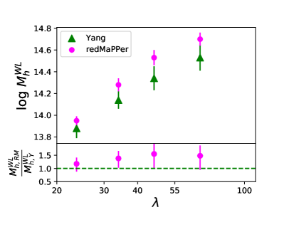
Figure 10: Similar to Figure 5, but for the weak lensing halo masses.

4.3 Halo Mass Comparison between Matched vs. Non-Matched Clusters

We start by measuring the overall $M_{h}^{\mathrm{WL}}$-$\lambda$ relations of the redMaPPer and Yang samples. Figure 9 shows the $\Delta\Sigma$ profiles of the redMaPPer (magenta circles with errorbars) and Yang (green squares with errorbars) clusters, binned by $\lambda$ in the same manner described in Section 2.4. In each panel, we show our fits (solid curves) over the radial range used from the $\Delta\Sigma$ profile to estimate the weak lensing halo mass, which is given at the bottom of each panel and shown in Figure 10. Our $M_{h}^{\mathrm{WL}}$ estimates are consistent with the similar measurements from Wang et al. (2022) and Simet et al. (2017) for the Yang and redMaPPer samples, respectively. Similar to Figure 5, the WL halo mass of the redMaPPer clusters is generally higher than that of the Yang clusters at fixed $\lambda$, though the difference is rather small at at $\lambda{<}30$. Since the effect of miscentring should be largely mitigated in the $\Delta\Sigma$ modelling, the discrepancy between the two $M_{h}^{\mathrm{WL}}$-$\lambda$ relations in Figure 10 should be primarily induced by the slightly larger scatter in our newly defined richness $\lambda_{\mathrm{Y}}$ for the Yang clusters compared to the original Yang richness and the redMaPPer richness.

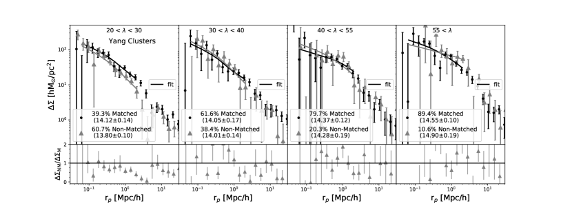
Figure 11: Comparison between the weak lensing profiles of the Yang clusters with matched counterparts in redMaPPer (dark circles with errorbars) and those without (gray triangles with errorbars) in four different richness bins. Dark and gray solid curves are the best-fitting model curves for the matched vs. non-matched clusters, respectively. The lower panels show the ratio between the two $\Delta\Sigma$ profiles.

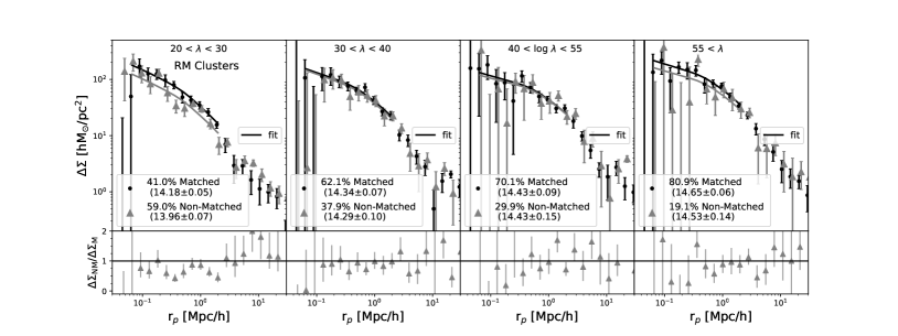
Figure 12: Similar to Figure 11, but for redMaPPer clusters that are split into matched vs. non-matched subsamples.

We now turn to the $\Delta\Sigma$ profiles of the matched vs. non-matched Yang clusters in the four bins of $\lambda$, as shown in Figure 11. In each panel, circles and triangles are the $\Delta\Sigma$ profiles of the matched and non-matched clusters, respectively, while dark and gray solid curves are the corresponding best-fitting model predictions. The WL halo mass estimates and the percentage of matched clusters within each bin are listed in the bottom of each top panel, with each bottom panel showing the ratios between the two $\Delta\Sigma$ profiles. The two sets of WL halo masses are largely consistent within $1\sigma$ for Yang clusters above $\lambda{=}30$, but differ by $\sim$1.4$\sigma$ in the lowest richness bin. In particular, the average log-halo mass of the matched clusters is $14.12{\pm}0.14$, $0.32$ dex higher than that of the non-matched clusters ($13.80{\pm}0.10$). This suggests that in the lowest-richness bin of the Yang catalogue, the redder clusters are likely more massive than the systems dominated by blue satellites. In the three higher richness bins, we do not detect any significant discrepancy between the two subsamples. Therefore, we expect that the Yang clusters should be largely free of systematic biases induced by the detection method if limited to clusters with $\lambda>30$ ($M_{h}^{\mathrm{WL}}{>}1.5\times 10^{14}h^{-1}M_{\odot}$).

Similarly, Figure 12 shows the result of the same analysis using the $\Delta\Sigma$ profiles of the matched vs. non-matched redMaPPer clusters. Across the three largest $\lambda$ bins, the average WL halo masses of the two subsamples are consistent with each other within 1$\sigma$, indicating that the preference of redMaPPer to select red-dominated clusters does not incur any significant systematic uncertainties in the scatter for clusters with $\lambda>30$ ($M_{h}^{\mathrm{WL}}{>}1.5\times 10^{14}h^{-1}M_{\odot}$), but differ by $\sim$1.8$\sigma$ in the lowest richness bin. In particular, the log-halo mass of matched clusters is $14.18{\pm}0.05$, $0.22$ dex higher than that of the non-matched clusters ($13.96{\pm}0.07$). This suggests that in the lowest-richness bin of the redMaPPer catalogue, there may exist a population of clusters with richnesses that have been artificially inflated as a result of projection effects in agreement with previous results (e.g., Wu et al., 2022; Wetzell et al., 2022). Interestingly, in the two low-$\lambda$ bins we find that the large-scale bias of the matched clusters is lower than that of the non-matched ones. This bias discrepancy at fixed WL halo mass is similar to the cluster assembly bias effect (Zu et al., 2021), although it could also be induced by a stronger projection effect in the non-matched subsample (Zu et al., 2017).

Overall, Figures 11 and  12 illustrate that when splitting the clusters into the matched and non-matched subsamples, the two WL halo masses at fixed $\lambda$ are always consistent with each other within $1\sigma$ for clusters with mass above $M_{h}^{\mathrm{WL}}{\simeq}1.5\times 10^{14}h^{-1}M_{\odot}$. This is encouraging news — despite the recognizable differences in the CLF shape between the Yang and redMaPPer cluster catalogues, our cluster weak lensing analysis exhibits no evidence for a strong systematic uncertainty in the scatter of the mass-richness relations in either cluster catalogue.

5 Conclusions

In this analysis, we focus on characterising the CLF and the WL halo masses for galaxy clusters identified using two different methodologies, the red-sequence (Rykoff et al., 2014) and halo-based method (Yang et al., 2021), using the overlapping volume at $0.1{<}z{<}0.34$ where both catalogues are complete. To mitigate the impact of different halo radius estimates, we adopt the same aperture ($1h^{-1}\mathrm{Mpc}$) to measure the richness and the CLFs for both cluster catalogues. In addition, we perform an abundance matching scheme over the two catalogues, to make sure the richness distributions of the two samples are the same above $\lambda=20$.

After thoroughly testing our stacking approach of measuring CLFs using a mock sample of photometric galaxies, we apply the method to the redMaPPer and Yang clusters by cross-correlating clusters with the SDSS photometric galaxy sample. We find mild differences in the total number of member galaxies with $M_{r}{<}-20.4$ between the two cluster catalogues, which is largely induced by the different random scatters in the respective mass-richness relations.

Focusing on the shape comparison between the CLFs of the two cluster samples at fixed $\lambda$, we observe modest differences in the behaviors of the two samples toward the faint end; redMaPPer clusters host more low-luminosity red satellites with a relatively flat population and Yang clusters contain a slightly declining population of fainter red galaxies. Meanwhile, Yang clusters exhibit a boosted population of blue galaxies at $M_{r}{<}{-}21$ compared to the redMaPPer clusters at the low richness. As a result, the red (blue) fraction of the redMaPPer clusters is higher (lower) than the Yang ones, especially at the low richness end.

To investigate the origin of the CLF shape discrepancy between the two clusters finders, we split the clusters from each catalogue at fixed $\lambda$ into two subsamples, one with matched counterparts in the other catalogue and the other without. The two sets of matched subsamples retain the same shape discrepancy exhibited by the overall sample, indicating that the discrepancy results largely from the clusters being assigned different centres. In particular, after we switch to the centres found by redMaPPer for the Yang clusters, we reproduce the flat/slightly increasing faint-end slope shown by the overall redMaPPer clusters. Therefore, for the first time we demonstrate that the overall shape and the faint-end slope of the CLF is sensitive to the centroiding algorithm employed by the optical cluster finders. Therefore, a robust scheme for mitigating miscentring is a prerequisite for any future study of the galaxy formation physics inside clusters using CLFs, whether it be direct or stacked measurements.

Strong colour preference in optical cluster finders does not necessarily translate into systematic biases in the scatter of the mass-richness relation of clusters. We investigate the latter using the same sets of matched vs. non-matched clusters in each catalogue, by taking advantage of the orthogonality in colour preference between the two cluster finders. In particular, if the average halo mass of the matched clusters is significantly different from that of the non-matched clusters at fixed $\lambda$, we would regard it as a strong evidence for the existence of systematic biases in the cluster catalogue. We estimate the average halo masses using the cluster weak lensing profiles measured from the DECaLS shear catalogue using Fourier_Quad (Zhang et al., 2015, 2019c; Zhang et al., 2022), by modelling the signal below $2h^{-1}\mathrm{Mpc}$ as the convolution between a projected NFW profile and a miscentring kernel function informed by the X-ray data (Zu et al., 2021). We do not find significant discrepancies between the weak lensing halo masses between the matched vs. non-matched clusters at halo mass above $M_{h}{\simeq}1.5*10^{14}h^{-1}M_{\odot}$ ($\lambda>30)$ for either cluster catalogue, suggesting that any systematic trend in the scatter of the mass-richness relation must be weak. However, at lower richnesses, we find discrepancies likely caused by either the inclusion of a large population of blue galaxies or the impact of projection effects (e.g., Zu et al., 2017; Wu et al., 2022; Wetzell et al., 2022) Therefore, the choice of how optical clusters are identified, whether by a red-sequence based or halo-based approach, should not impact cluster cosmological analyses, if the clusters with $M_{h}<1.5*10^{14}h^{-1}M_{\odot}$ are excluded.

Although we do not find strong evidence of systematic uncertainties due to the CLF preference of cluster finders at $z{<}0.34$, it is unclear whether detection bias would plague future cluster surveys at higher redshifts. In particular, the Rubin Observatory Legacy Survey of Space and Time (LSST; Ivezić et al., 2019), the China Space Station Telescope (CSST; Gong et al., 2019), and the Roman Space Telescope (Roman; Spergel et al., 2015) will allow us to detect clusters out to $z\approx 1.5$ (Ivezić et al., 2019). Although high-redshift clusters and proto-clusters have been identified out to $z>1.5$ (e.g., Cerulo et al., 2016; Cooke et al., 2016; Golden-Marx et al., 2019; Willis et al., 2020; Li et al., 2022) many of the clusters identified at $z>1$ will look different than their low-redshift counterparts, and not all will be characterized by a strong red sequence (Brodwin et al., 2013). Therefore, it is important to keep pushing our finder comparison to higher redshifts, in order to thoroughly understand the systematics and nuances of the different methods of identifying galaxy clusters for LSST, CSST, and Roman.

Going forward, there are many avenues of inquiry that we aim to explore building off the analysis presented here. In the near future, we plan to continue to investigate the CLF, including its central galaxy component, as we investigate whether the CLF can inform BCG hierarchical growth. We plan to split the CLF by magnitude gap, the difference in brightness between the BCG and nth brightest cluster member. As found in Golden-Marx & Miller (2018) the magnitude gap is an observational proxy for hierarchical assembly so this split may allow us to infer the properties of the progenitors of BCGs. Additionally, we plan to perform radial splits to determine whether there exists an observational signature of the BCG “sphere of influence” identified by Chen et al. (2022) in the galaxy population. In the future, we plan to improve the CLF and WL measurements by incorporating the spectroscopic data from DESI (Abareshi et al., 2022) and centring information from eROSITA (Predehl et al., 2021), thereby allowing us to better constrain cluster identification and properties as we enter the era of CSST, LSST, and Roman.

Data availability

The data underlying this article will be shared on reasonable request to the corresponding author.

Appendix A CLF Parameters of Matched vs. Non-Matched Subsamples

In Table 3, we present the CLF parameters for the Yang subsamples with and without a cross-match. In Table 4, we present the CLF parameters for the redMaPPer subsamples with and without a cross-match.

Table 3: Best-fitting CLF parameters of the Yang cluster subsamples in Figure 7. Ycen or RMcen indicates that the Yang or redMaPPer centres are adopted for the CLF measurement.

bin	M∗	$\alpha$	$\phi^{*}$
All galaxies of Matched Yang clusters (Ycen)
1	-22.05 $\pm$ 0.06	-1.07 $\pm$ 0.03	2.42 $\pm$ 0.13
2	-21.73 $\pm$ 0.05	-0.91 $\pm$ 0.03	4.28 $\pm$ 0.21
3	-21.63 $\pm$ 0.06	-0.87 $\pm$ 0.04	5.49 $\pm$ 0.29
4	-21.65 $\pm$ 0.06	-0.90 $\pm$ 0.04	6.68 $\pm$ 0.40
Red galaxies of Matched Yang clusters (Ycen)
1	-21.95 $\pm$ 0.05	-0.93 $\pm$ 0.03	2.58 $\pm$ 0.12
2	-21.65 $\pm$ 0.05	-0.78 $\pm$ 0.03	4.28 $\pm$ 0.18
3	-21.62 $\pm$ 0.06	-0.79 $\pm$ 0.04	5.15 $\pm$ 0.25
4	-21.60 $\pm$ 0.06	-0.79 $\pm$ 0.04	6.56 $\pm$ 0.36
Blue galaxies of Matched Yang clusters (Ycen)
1	-21.62 $\pm$ 0.23	-1.56 $\pm$ 0.08	0.24 $\pm$ 0.07
2	-21.48 $\pm$ 0.25	-1.42 $\pm$ 0.11	0.40 $\pm$ 0.13
3	-21.36 $\pm$ 0.23	-1.33 $\pm$ 0.12	0.54 $\pm$ 0.15
4	-21.22 $\pm$ 0.30	-1.35 $\pm$ 0.16	0.65 $\pm$ 0.24
All galaxies of Matched Yang clusters (RMcen)
1	-22.28 $\pm$ 0.08	-1.21 $\pm$ 0.04	1.95 $\pm$ 0.18
2	-21.91 $\pm$ 0.07	-1.07 $\pm$ 0.04	3.43 $\pm$ 0.26
3	-21.79 $\pm$ 0.07	-1.01 $\pm$ 0.04	4.43 $\pm$ 0.32
4	-21.72 $\pm$ 0.08	-0.97 $\pm$ 0.05	5.97 $\pm$ 0.53
Red galaxies of Matched Yang clusters (RMcen)
1	-22.21 $\pm$ 0.07	-1.11 $\pm$ 0.04	2.05 $\pm$ 0.17
2	-21.86 $\pm$ 0.06	-0.95 $\pm$ 0.04	3.50 $\pm$ 0.23
3	-21.79 $\pm$ 0.07	-0.94 $\pm$ 0.04	4.16 $\pm$ 0.29
4	-21.63 $\pm$ 0.08	-0.86 $\pm$ 0.05	6.11 $\pm$ 0.49
Blue galaxies of Matched Yang clusters (RMcen)
1	-21.51 $\pm$ 0.31	-1.62 $\pm$ 0.11	0.23 $\pm$ 0.10
2	-21.25 $\pm$ 0.28	-1.43 $\pm$ 0.13	0.44 $\pm$ 0.16
3	-21.32 $\pm$ 0.25	-1.41 $\pm$ 0.12	0.46 $\pm$ 0.15
4	-21.58 $\pm$ 0.36	-1.54 $\pm$ 0.14	0.35 $\pm$ 0.18
All galaxies of Non-Matched Yang clusters
1	-21.96 $\pm$ 0.05	-0.90 $\pm$ 0.03	2.52 $\pm$ 0.11
2	-21.54 $\pm$ 0.06	-0.69 $\pm$ 0.05	4.87 $\pm$ 0.25
3	-21.65 $\pm$ 0.12	-0.85 $\pm$ 0.08	5.33 $\pm$ 0.60
4	-21.57 $\pm$ 0.22	-0.79 $\pm$ 0.17	6.70 $\pm$ 1.35
Red galaxies of Non-Matched Yang clusters
1	-21.86 $\pm$ 0.04	-0.72 $\pm$ 0.03	2.53 $\pm$ 0.09
2	-21.50 $\pm$ 0.06	-0.52 $\pm$ 0.05	4.54 $\pm$ 0.20
3	-21.59 $\pm$ 0.12	-0.69 $\pm$ 0.09	5.02 $\pm$ 0.49
4	-21.39 $\pm$ 0.22	-0.61 $\pm$ 0.18	7.11 $\pm$ 1.18
Blue galaxies of Non-Matched Yang clusters
1	-21.67 $\pm$ 0.17	-1.44 $\pm$ 0.06	0.31 $\pm$ 0.06
2	-20.98 $\pm$ 0.22	-1.03 $\pm$ 0.17	0.87 $\pm$ 0.21
3	-21.14 $\pm$ 0.44	-1.21 $\pm$ 0.27	0.93 $\pm$ 0.45
4	-20.94 $\pm$ 0.96	-1.03 $\pm$ 0.68	0.75 $\pm$ 1.20

Table 4: Best-fitting CLF parameters of the redMaPPer cluster subsamples in Figure 8. Ycen or RMcen indicates that the Yang or redMaPPer centres are adopted for the CLF measurement.

bin	M∗	$\alpha$	$\phi^{*}$
All galaxies of Matched redMaPPer clusters (RMcen)
1	-22.00 $\pm$ 0.05	-1.06 $\pm$ 0.03	2.71 $\pm$ 0.15
2	-21.93 $\pm$ 0.05	-1.08 $\pm$ 0.02	3.57 $\pm$ 0.20
3	-21.85 $\pm$ 0.06	-1.09 $\pm$ 0.03	4.63 $\pm$ 0.29
4	-21.77 $\pm$ 0.06	-1.05 $\pm$ 0.03	6.85 $\pm$ 0.48
Red galaxies of Matched redMaPPer clusters (RMcen)
1	-21.94 $\pm$ 0.05	-0.94 $\pm$ 0.03	2.77 $\pm$ 0.13
2	-21.86 $\pm$ 0.05	-0.96 $\pm$ 0.03	3.66 $\pm$ 0.18
3	-21.75 $\pm$ 0.06	-0.97 $\pm$ 0.03	4.99 $\pm$ 0.29
4	-21.72 $\pm$ 0.06	-0.95 $\pm$ 0.03	7.00 $\pm$ 0.45
Blue galaxies of Matched redMaPPer clusters (RMcen)
1	-21.57 $\pm$ 0.26	-1.56 $\pm$ 0.10	0.25 $\pm$ 0.09
2	-21.23 $\pm$ 0.26	-1.41 $\pm$ 0.13	0.48 $\pm$ 0.16
3	-21.56 $\pm$ 0.33	-1.67 $\pm$ 0.11	0.30 $\pm$ 0.14
4	-21.44 $\pm$ 0.33	-1.59 $\pm$ 0.12	0.42 $\pm$ 0.19
All galaxies of Matched redMaPPer clusters (Ycen)
1	-21.93 $\pm$ 0.04	-0.96 $\pm$ 0.02	3.12 $\pm$ 0.13
2	-21.91 $\pm$ 0.05	-0.99 $\pm$ 0.03	3.74 $\pm$ 0.19
3	-21.74 $\pm$ 0.06	-0.99 $\pm$ 0.03	5.09 $\pm$ 0.30
4	-21.58 $\pm$ 0.07	-0.93 $\pm$ 0.04	7.36 $\pm$ 0.48
Red galaxies of Matched redMaPPer clusters (Ycen)
1	-21.84 $\pm$ 0.04	-0.81 $\pm$ 0.02	3.22 $\pm$ 0.12
2	-21.83 $\pm$ 0.05	-0.87 $\pm$ 0.03	3.81 $\pm$ 0.16
3	-21.68 $\pm$ 0.05	-0.87 $\pm$ 0.03	5.14 $\pm$ 0.26
4	-21.45 $\pm$ 0.07	-0.77 $\pm$ 0.04	7.85 $\pm$ 0.45
Blue galaxies of Matched redMaPPer clusters (Ycen)
1	-21.46 $\pm$ 0.18	-1.42 $\pm$ 0.08	0.36 $\pm$ 0.08
2	-21.43 $\pm$ 0.25	-1.44 $\pm$ 0.11	0.41 $\pm$ 0.13
3	-21.68 $\pm$ 0.30	-1.56 $\pm$ 0.11	0.33 $\pm$ 0.13
4	-21.40 $\pm$ 0.29	-1.56 $\pm$ 0.11	0.48 $\pm$ 0.19
All galaxies of Non-Matched redMaPPer clusters
1	-22.15 $\pm$ 0.05	-1.19 $\pm$ 0.02	1.92 $\pm$ 0.12
2	-21.96 $\pm$ 0.08	-1.11 $\pm$ 0.03	3.25 $\pm$ 0.26
3	-21.75 $\pm$ 0.09	-1.10 $\pm$ 0.04	4.91 $\pm$ 0.47
4	-21.75 $\pm$ 0.11	-1.08 $\pm$ 0.05	6.90 $\pm$ 0.76
Red galaxies of Non-Matched redMaPPer clusters
1	-22.06 $\pm$ 0.05	-1.05 $\pm$ 0.02	2.13 $\pm$ 0.11
2	-21.80 $\pm$ 0.07	-0.95 $\pm$ 0.04	3.67 $\pm$ 0.25
3	-21.64 $\pm$ 0.08	-0.97 $\pm$ 0.04	5.19 $\pm$ 0.55
4	-21.64 $\pm$ 0.10	-0.95 $\pm$ 0.05	7.40 $\pm$ 0.93
Blue galaxies of Non-Matched redMaPPer clusters
1	-20.75 $\pm$ 0.24	-1.51 $\pm$ 0.11	0.49 $\pm$ 0.16
2	-21.43 $\pm$ 0.50	-1.67 $\pm$ 0.13	0.27 $\pm$ 0.18
3	-21.00 $\pm$ 0.43	-1.39 $\pm$ 0.19	0.77 $\pm$ 0.44
4	-21.00 $\pm$ 0.64	-1.59 $\pm$ 0.24	0.78 $\pm$ 0.70

Appendix B Theoretical Model of $\Delta\Sigma$

In this analysis, we use a Bayesian framework to infer $M_{h}^{\mathrm{WL}}$ directly from the $\Delta\Sigma$ profiles, following the same mathematical formalism as outlined in Zu et al. (2021), which are computed as

$$\Delta\Sigma(r_{p})=\overline{\Sigma}({<}r_{p})-\Sigma(r_{p}),$$ (2)

where $\overline{\Sigma}({<}r_{p})$ and $\Sigma(r_{p})$ are the average surface matter density within and at the projected radius r_p. Without miscentring, $\Sigma(r_{p})$ can be computed from the 3D isotropic halo-matter cross-correlation function $\xi_{\rm hm}(r)$,

$$\Sigma(r_{p})=\rho_{m}\int_{-\infty}^{+\infty}\xi_{\rm hm}(r_{p},r_{\pi})dr_{\pi},$$ (3)

where $\rho_{m}$ is the mean density of the Universe.

To model the effect of miscentring, we assume that the fraction of miscentred BCGs is $f_{\rm off}$ with an offset of $\sigma_{\rm off}$ from the true cluster centre and that this distribution follows a shape-2 Gamma distribution $p(r_{\rm off})$ with a characteristic offset $\sigma_{\rm off}$,

$$p(r_{\rm off})=\frac{r_{\rm off}}{\sigma_{\rm off}^{2}}\exp\left(-\frac{r_{\rm off}}{\sigma_{\rm off}}\right).$$ (4)

Thus, the observed surface matter density profile when accounting for miscentring can be written as

$$\Sigma^{\rm obs}(r_{p})=f_{\rm off}\Sigma^{\rm off}(r_{p})+(1-f_{\rm off})\Sigma(r_{p}),$$ (5)

where

$$\begin{split}\Sigma^{\rm off}(r_{p})=&\frac{1}{2\pi}\int_{0}^{\infty}dr_{\rm off}p(r_{\rm off})\\ &\times\int_{0}^{2\pi}d\theta\Sigma(\sqrt{r_{p}^{2}+r_{\rm off}^{2}-2r_{p}r_{\rm off}^{2}}\cos{\theta})\end{split}\\$$ (6)

The purpose of this weak lensing analysis is to compare the average halo masses of different cluster samples, which are primarily inferred from $\Delta\Sigma$ on scales below $2h^{-1}\mathrm{Mpc}$ (Zu et al., 2014). Therefore, we only model $\xi_{\rm 1h}$, the “1-halo” term of $\xi_{\rm hm}$, for predicting $\Delta\Sigma$ at $r_{p}{<}2h^{-1}\mathrm{Mpc}$ Zu et al. (2014)

$$\xi_{\rm 1h}=\frac{\rho_{\mathrm{NFW}}(r|M_{h})}{\rho_{m}}-1,$$ (7)

where $\rho_{\mathrm{NFW}}$ is the NFW density profile. Additionally, we fit to the observed $\Delta\Sigma$ down to a minimum scale of $r_{p}=0.1h^{-1}\mathrm{Mpc}$, below which the extra lensing effect caused by the stellar mass of the BCG needs to be incorporated.

B.1 WL Parameters

In Tables 5 and 6, we present the 1D posterior distributions for the fitting to the $\Delta\Sigma$ profiles used to estimate $M_{h}^{\mathrm{WL}}$.

Table 5: Best-fitting WL model parameters of the Yang cluster subsamples in Figures 9 and  11.

bin	log $M_{h}^{\mathrm{WL}}$	c	$\sigma_{\mathrm{off}}$	foff
Overall Yang clusters
1	13.89 $\pm$ 0.09	5.06 $\pm$ 1.15	0.43 $\pm$ 0.30	0.23 $\pm$ 0.13
2	14.14 $\pm$ 0.08	4.58 $\pm$ 1.30	0.43 $\pm$ 0.31	0.35 $\pm$ 0.18
3	14.34 $\pm$ 0.11	4.08 $\pm$ 1.52	0.31 $\pm$ 0.25	0.52 $\pm$ 0.24
4	14.53 $\pm$ 0.12	4.79 $\pm$ 1.27	0.50 $\pm$ 0.31	0.42 $\pm$ 0.17
Matched Yang clusters
1	14.12 $\pm$ 0.14	5.18 $\pm$ 1.21	0.52 $\pm$ 0.29	0.31 $\pm$ 0.19
2	14.05 $\pm$ 0.17	5.36 $\pm$ 1.29	0.52 $\pm$ 0.29	0.31 $\pm$ 0.19
3	14.37 $\pm$ 0.12	4.50 $\pm$ 1.46	0.26 $\pm$ 0.25	0.52 $\pm$ 0.22
4	14.55 $\pm$ 0.10	4.00 $\pm$ 1.03	0.42 $\pm$ 0.26	0.34 $\pm$ 0.15
Non-Matched Yang clusters
1	13.80 $\pm$ 0.10	5.02 $\pm$ 1.22	0.45 $\pm$ 0.30	0.21 $\pm$ 0.14
2	14.01 $\pm$ 0.14	5.31 $\pm$ 1.20	0.52 $\pm$ 0.31	0.17 $\pm$ 0.15
3	14.28 $\pm$ 0.19	4.50 $\pm$ 1.36	0.39 $\pm$ 0.29	0.29 $\pm$ 0.21
4	14.90 $\pm$ 0.19	4.76 $\pm$ 1.36	0.49 $\pm$ 0.30	0.59 $\pm$ 0.23

Table 6: Best-fitting WL model parameters of the redMaPPer cluster samples in Figures 9 and  12.

bin	$\log M_{h}^{\mathrm{WL}}$	c	$\sigma_{\mathrm{off}}$	foff
Overall redMaPPer clusters
1	13.95 $\pm$ 0.04	7.09 $\pm$ 0.90	0.18 $\pm$ 0.02	0.27 $\pm$ 0.04
2	14.28 $\pm$ 0.06	5.24 $\pm$ 0.88	0.18 $\pm$ 0.02	0.30 $\pm$ 0.04
3	14.53 $\pm$ 0.07	3.65 $\pm$ 0.75	0.18 $\pm$ 0.02	0.31 $\pm$ 0.04
4	14.70 $\pm$ 0.06	4.88 $\pm$ 0.82	0.18 $\pm$ 0.02	0.17 $\pm$ 0.04
Matched redMaPPer clusters
1	14.18 $\pm$ 0.05	5.81 $\pm$ 0.90	0.18 $\pm$ 0.02	0.30 $\pm$ 0.04
2	14.34 $\pm$ 0.07	4.62 $\pm$ 0.95	0.18 $\pm$ 0.02	0.30 $\pm$ 0.04
3	14.43 $\pm$ 0.09	3.84 $\pm$ 1.01	0.18 $\pm$ 0.02	0.31 $\pm$ 0.04
4	14.65 $\pm$ 0.06	4.98 $\pm$ 0.84	0.18 $\pm$ 0.02	0.30 $\pm$ 0.04
Non-Matched redMaPPer clusters
1	13.96 $\pm$ 0.07	5.00 $\pm$ 0.94	0.18 $\pm$ 0.02	0.30 $\pm$ 0.04
2	14.29 $\pm$ 0.10	4.61 $\pm$ 1.16	0.18 $\pm$ 0.18	0.31 $\pm$ 0.04
3	14.43 $\pm$ 0.15	3.51 $\pm$ 1.10	0.18 $\pm$ 0.02	0.28 $\pm$ 0.04
4	14.53 $\pm$ 0.14	5.40 $\pm$ 1.02	0.18 $\pm$ 0.02	0.30 $\pm$ 0.04

References

- Abareshi et al. (2022) Abareshi B., et al., 2022, AJ, 164, 207
- Abbott et al. (2018) Abbott T. M. C., et al., 2018, Phys. Rev. D, 98, 043526
- Abbott et al. (2020) Abbott T. M. C., et al., 2020, Phys. Rev. D, 102, 023509
- Ahumada et al. (2020) Ahumada R., et al., 2020, ApJS, 249, 3
- Aihara et al. (2011) Aihara H., et al., 2011, ApJS, 195, 26
- Alam et al. (2017) Alam S., et al., 2017, MNRAS, 470, 2617
- Beutler et al. (2011) Beutler F., et al., 2011, MNRAS, 416, 3017
- Birnboim & Dekel (2003) Birnboim Y., Dekel A., 2003, MNRAS, 345, 349
- Bocquet et al. (2019) Bocquet S., et al., 2019, ApJ, 878, 55
- Brodwin et al. (2013) Brodwin M., et al., 2013, ApJ, 779, 138
- Busch & White (2017) Busch P., White S. D. M., 2017, MNRAS, 470, 4767
- Cerulo et al. (2016) Cerulo P., et al., 2016, MNRAS, 457, 2209
- Chen et al. (2022) Chen X., Zu Y., Shao Z., Shan H., 2022, MNRAS, 514, 2692
- Chiu et al. (2022) Chiu I.-N., Klein M., Mohr J., Bocquet S., 2022, arXiv e-prints, p. arXiv:2207.12429
- Cooke et al. (2016) Cooke E. A., et al., 2016, ApJ, 816, 83
- Costanzi et al. (2021) Costanzi M., et al., 2021, Phys. Rev. D, 103, 043522
- Dalal et al. (2008) Dalal N., White M., Bond J. R., Shirokov A., 2008, ApJ, 687, 12
- Dey et al. (2019) Dey A., et al., 2019, AJ, 157, 168
- Gao & White (2007) Gao L., White S. D. M., 2007, MNRAS, 377, L5
- Gao et al. (2005) Gao L., Springel V., White S. D. M., 2005, MNRAS, 363, L66
- George et al. (2012) George M. R., et al., 2012, ApJ, 757, 2
- Gladders & Yee (2000) Gladders M. D., Yee H. K. C., 2000, AJ, 120, 2148
- Gladders & Yee (2005) Gladders M. D., Yee H. K. C., 2005, ApJS, 157, 1
- Golden-Marx & Miller (2018) Golden-Marx J. B., Miller C. J., 2018, ApJ, 860, 2
- Golden-Marx et al. (2019) Golden-Marx E., et al., 2019, ApJ, 887, 50
- Gong et al. (2019) Gong Y., et al., 2019, ApJ, 883, 203
- Groenewald et al. (2017) Groenewald D. N., Skelton R. E., Gilbank D. G., Loubser S. I., 2017, MNRAS, 467, 4101
- Hansen et al. (2009) Hansen S. M., Sheldon E. S., Wechsler R. H., Koester B. P., 2009, ApJ, 699, 1333
- Hollowood et al. (2019) Hollowood D. L., et al., 2019, ApJS, 244, 22
- Ivezić et al. (2019) Ivezić Ž., et al., 2019, ApJ, 873, 111
- Jing et al. (2007) Jing Y. P., Suto Y., Mo H. J., 2007, ApJ, 657, 664
- Johnston et al. (2007) Johnston D. E., Sheldon E. S., Tasitsiomi A., Frieman J. A., Wechsler R. H., McKay T. A., 2007, ApJ, 656, 27
- Koester et al. (2007) Koester B. P., et al., 2007, ApJ, 660, 239
- Lan et al. (2016) Lan T.-W., Ménard B., Mo H., 2016, MNRAS, 459, 3998
- Li et al. (2022) Li Q., et al., 2022, ApJ, 933, 9
- Mantz et al. (2015) Mantz A. B., et al., 2015, MNRAS, 446, 2205
- Meng et al. (2022) Meng J., Li C., Mo H., Chen Y., Jiang Z., Xie L., 2022, arXiv e-prints, p. arXiv:2210.17186
- Miller et al. (2005) Miller C. J., et al., 2005, AJ, 130, 968
- Myles et al. (2021) Myles J., et al., 2021, MNRAS, 505, 33
- Navarro et al. (1997) Navarro J. F., Frenk C. S., White S. D. M., 1997, ApJ, 490, 493
- Park et al. (2021) Park Y., Sunayama T., Takada M., Kobayashi Y., Miyatake H., More S., Nishimichi T., Sugiyama S., 2021, arXiv e-prints, p. arXiv:2112.09059
- Planck Collaboration et al. (2020) Planck Collaboration et al., 2020, A&A, 641, A6
- Predehl et al. (2021) Predehl P., et al., 2021, A&A, 647, A1
- Rozo et al. (2010) Rozo E., et al., 2010, ApJ, 708, 645
- Rozo et al. (2015) Rozo E., Rykoff E. S., Becker M., Reddick R. M., Wechsler R. H., 2015, MNRAS, 453, 38
- Rykoff et al. (2012) Rykoff E. S., et al., 2012, ApJ, 746, 178
- Rykoff et al. (2014) Rykoff E. S., et al., 2014, ApJ, 785, 104
- Rykoff et al. (2016) Rykoff E. S., et al., 2016, ApJS, 224, 1
- Salcedo et al. (2022) Salcedo A. N., et al., 2022, Science China Physics, Mechanics, and Astronomy, 65, 109811
- Schechter (1976) Schechter P., 1976, ApJ, 203, 297
- Simet et al. (2017) Simet M., McClintock T., Mandelbaum R., Rozo E., Rykoff E., Sheldon E., Wechsler R. H., 2017, MNRAS, 466, 3103
- Spergel et al. (2015) Spergel D., et al., 2015, arXiv e-prints, p. arXiv:1503.03757
- Sunayama et al. (2020) Sunayama T., et al., 2020, MNRAS, 496, 4468
- Tinker (2021) Tinker J. L., 2021, ApJ, 923, 154
- Tinker (2022) Tinker J. L., 2022, AJ, 163, 126
- Tinker et al. (2012) Tinker J. L., et al., 2012, ApJ, 745, 16
- Tinker et al. (2021) Tinker J. L., Cao J., Alpaslan M., DeRose J., Mao Y.-Y., Wechsler R. H., 2021, MNRAS, 505, 5370
- To et al. (2020) To C.-H., Reddick R. M., Rozo E., Rykoff E., Wechsler R. H., 2020, ApJ, 897, 15
- Wang et al. (2016) Wang H., et al., 2016, ApJ, 831, 164
- Wang et al. (2022) Wang J., et al., 2022, ApJ, 936, 161
- Weinberg et al. (2013) Weinberg D. H., Mortonson M. J., Eisenstein D. J., Hirata C., Riess A. G., Rozo E., 2013, Phys. Rep., 530, 87
- Wen et al. (2012) Wen Z. L., Han J. L., Liu F. S., 2012, ApJS, 199, 34
- Wetzell et al. (2022) Wetzell V., et al., 2022, MNRAS, 514, 4696
- Willis et al. (2020) Willis J. P., et al., 2020, Nature, 577, 39
- Wu et al. (2022) Wu H.-Y., et al., 2022, MNRAS, 515, 4471
- Yang et al. (2003) Yang X., Mo H. J., van den Bosch F. C., 2003, MNRAS, 339, 1057
- Yang et al. (2005) Yang X., Mo H. J., van den Bosch F. C., Jing Y. P., 2005, MNRAS, 356, 1293
- Yang et al. (2007) Yang X., Mo H. J., van den Bosch F. C., Pasquali A., Li C., Barden M., 2007, ApJ, 671, 153
- Yang et al. (2008) Yang X., Mo H. J., van den Bosch F. C., 2008, ApJ, 676, 248
- Yang et al. (2021) Yang X., et al., 2021, ApJ, 909, 143
- York et al. (2000) York D. G., et al., 2000, AJ, 120, 1579
- Zeng et al. (2022) Zeng C., Salcedo A. N., Wu H.-Y., Hirata C. M., 2022, arXiv e-prints, p. arXiv:2210.16306
- Zhang et al. (2015) Zhang J., Luo W., Foucaud S., 2015, J. Cosmology Astropart. Phys., 2015, 024
- Zhang et al. (2019a) Zhang Y., et al., 2019a, MNRAS, 487, 2578
- Zhang et al. (2019b) Zhang Y., et al., 2019b, MNRAS, 488, 1
- Zhang et al. (2019c) Zhang J., et al., 2019c, ApJ, 875, 48
- Zhang et al. (2022) Zhang J., Liu C., Vaquero P. A., Li H., Wang H., Shen Z., Dong F., 2022, AJ, 164, 128
- Zhou et al. (2021) Zhou R., et al., 2021, MNRAS, 501, 3309
- Zou et al. (2019) Zou H., Gao J., Zhou X., Kong X., 2019, ApJS, 242, 8
- Zou et al. (2021) Zou H., et al., 2021, ApJS, 253, 56
- Zu & Mandelbaum (2015) Zu Y., Mandelbaum R., 2015, MNRAS, 454, 1161
- Zu et al. (2014) Zu Y., Weinberg D. H., Rozo E., Sheldon E. S., Tinker J. L., Becker M. R., 2014, MNRAS, 439, 1628
- Zu et al. (2017) Zu Y., Mandelbaum R., Simet M., Rozo E., Rykoff E. S., 2017, MNRAS, 470, 551
- Zu et al. (2021) Zu Y., et al., 2021, MNRAS, 505, 5117
- Zu et al. (2022) Zu Y., et al., 2022, MNRAS, 511, 1789