Cosmological Dark Matter from a Bulk Black Hole

Abstract

We study the cosmology of a three-brane in a specific five-dimensional scalar-gravity (i.e. soft-wall) background, known as the linear dilaton background. We discover that the Friedmann equation of the brane-world automatically contains a term mimicking pressureless matter. We propose to identify this term as dark matter. This dark matter arises as a projection of the bulk black hole on the brane, which contributes to the brane Friedmann equation via both the Weyl tensor and the scalar stress tensor. The nontrivial matter-like behavior is due to an exact cancellation between the Weyl and scalar pressures. We show that the Newtonian potential only receives a mild short-distance correction going as inverse distance squared, ensuring compatibility of the linear dilaton brane-world with observed 4D gravity. Our setup can be viewed as a consistent cosmological description of the holographic theories arising in the linear dilaton background. We also present more general scalar-gravity models where the brane cosmology features an effective energy density whose behavior smoothly interpolates between dark radiation, dark matter and dark energy depending on a model parameter.

I Introduction

Five-dimensional (5D) gravity coupled to a scalar field has proven to be a fecund playground, leading to a host of theoretical results and models of the real world (see e.g. Karch et al. (2006); Gursoy and Kiritsis (2008); Gursoy et al. (2008); Gubser and Nellore (2008); Falkowski and Perez-Victoria (2008); Batell and Gherghetta (2008); Batell et al. (2008); Cabrer et al. (2010); von Gersdorff (2010); Cabrer et al. (2011); Megías and Quirós (2019, 2021a, 2021b)). Our focus in this letter is a specific 5D scalar-gravity background (i.e. a soft-wall background) which is sometimes referred to as the “linear dilaton background”. This model is known to have peculiar thermodynamic Gursoy and Kiritsis (2008) and field theoretical properties Cabrer et al. (2010); Megías and Quirós (2019, 2021a, 2021b). For example, all quantum fields living on the linear dilaton background have a spectral distribution that features a gapped continuum. This feature has been recently used in extensions of the Standard Model Csáki et al. (2022a, b).

In this work we put the linear dilaton background at finite temperature and posit a flat 3-brane moving over the background, in the spirit of brane-world models (see e.g. Brax and van de Bruck (2003)). We discover a surprising property: from the viewpoint of a brane observer, the local Friedmann equation automatically contains an effective energy term that may be identified as dark matter. This dark matter emerges as a nontrivial effect from the bulk physics projected on the brane. It originates from a combination of the 5D Weyl tensor and of the bulk scalar vev, as we will demonstrate further below.

To bring this result into context, we remind that there is a notorious analog in pure Anti-de Sitter (AdS) background, that has been gradually uncovered and studied in Shiromizu et al. (2000); Binetruy et al. (2000); Hebecker and March-Russell (2001); Langlois et al. (2002); Langlois and Sorbo (2003). In pure AdS the net effect of the bulk physics projected on the brane gives rise to radiation, which is identified as cosmological dark radiation in the context of a brane-world. This remarkable fact is in direct connection with the fact that the bulk black hole in AdS-Schwarzschild background corresponds to the thermal state in the holographic CFT, perhaps one of the most fascinating entries of the AdS/CFT correspondence Aharony et al. (2000). In our case, by performing the analogous calculation with the linear dilaton background, we discover that the bulk black hole gives rise to dark matter.

Decades of astronomical observations point to the existence of dark matter. Determining its nature is a pressing question in fundamental physics. While a common hypothesis is that dark matter may be a new particle (that remains so far elusive), our study leads to a fundamentally different viewpoint. Our setup provides, in a sense, an origin to cosmological dark matter via a modification of gravity. See e.g. Clifton et al. (2012) for a few other attempts to explain dark matter via modified gravity.

In this paper we present the derivation of our central result, the effective Friedmann equation of the linear dilaton brane-world, that is shown to contain dark matter. We present nontrivial consistency checks of this result. We also compute the deviation to the Newtonian potential. We then outline more general models featuring a variety of equations of state depending on a model parameter, and discuss some conceptual points and prospects. Extra developments and technical details are laid out in Fichet et al. (2022), which can be considered as a companion to this letter.

II The 5D scalar-gravity system

We consider the general scalar-gravity action in the presence of a brane,

$$S = \int d^{5}x\sqrt{g}\left(\frac{M_{5}^{3}}{2}{}^{(5)}R-\frac{1}{2}(\partial_{M}\phi)^{2}-V(\phi)\right)$$ (1)

$$- \int_{\textrm{brane}}d^{4}x\sqrt{\bar{g}}\,(V_{b}(\phi)+\Lambda_{b})+\ldots\,$$

${}^{(5)}R$ is the 5D Ricci scalar, $\phi$ is the scalar field, $M_{5}$ is the fundamental 5D Planck scale, $\bar{g}_{\mu\nu}$ is the induced metric on the brane, $g\equiv|\det g_{MN}|$ and $\bar{g}\equiv|\det\bar{g}_{\mu\nu}|$ are the metrics determinants, $\Lambda_{b}$ is the brane tension, $V$ and $V_{b}$ are the bulk and brane-localized potentials for $\phi$. We assume that the brane potential sets the scalar field vacuum expectation value (vev) to a nonzero value $\langle\phi\rangle=v_{b}$, with $V_{b}(v_{b})=0$. The bulk potential is explicitly given further below. The ellipses encode the Gibbons-Hawking-York term York (1972); Gibbons and Hawking (1977) and the action of quantum fields living on the 5D background.

The 5D metric is written in a frame suitable for brane cosmology as

$$ds^{2} =g_{MN}dx^{M}dx^{N}\equiv-n^{2}(r)d\tau^{2}+\frac{r^{2}}{\ell^{2}}d\mathbf{x}^{2}+b^{2}(r)dr^{2}\,.$$ (2)

We allow the existence of a black hole horizon encoded in the $n(r)$ and $b(r)$ factors, the position of the horizon being given by $n(r_{h})=0=1/b(r_{h})$. Latin indices $(M,N,\cdots)$ refer to 5D coordinates, Greek indices $(\mu,\nu,\cdots)$ refer to 4D coordinates.

The 3-brane is localized at the position $r=r_{b}$. Our frame (2) is appropriate to describe cosmology as seen from the brane standpoint. The induced metric on the brane is

$$ds^{2} =\bar{g}_{\mu\nu}dx^{\mu}dx^{\nu}\equiv-dt^{2}+\frac{r_{b}^{2}}{\ell^{2}}d\mathbf{x}^{2}\,,$$ (3)

where we have introduced the brane cosmic time $dt=n(r_{b})d\tau$. According to this metric, if the brane moves along $r$ in the 5D background, the observer perceives expansion of the four-dimensional (4D) universe with Hubble parameter $H=\dot{r_{b}}/r_{b}$, where $\dot{r_{b}}\equiv\partial_{t}r_{b}$. We choose that $r_{b}$ equals $\ell$ at present times, such that $r_{b}=a(t)\ell$ where $a(t)$ is the standard scale factor. An overview of the brane-world is shown in Fig. 1.

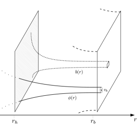
Figure 1: Overview of the scalar-gravity system. The brane and the horizon are located respectively at $r=r_{b}$ and $r=r_{h}$. The scalar vacuum expectation value is fixed by a brane potential to a value $v_{b}$ which remains constant when $r_{b}$ varies. The scalar VEV (plain) evolves in the bulk, the blackening factor of the metric (dotted) diverges at the horizon.

The 5D equations of motion of the system are

$${}^{(5)}G_{MN}=\frac{1}{M_{5}^{3}}T^{\phi}_{MN}\,,\quad\frac{1}{\sqrt{g}}\partial_{M}\left(\sqrt{g}g^{MN}\partial_{N}\phi\right)=\frac{\partial V}{\partial\phi}\,,$$ (4)

with ${}^{(5)}G_{MN}={}^{(5)}R_{MN}-\frac{1}{2}g_{MN}{}^{(5)}R$ and $T^{\phi}_{MN}=\partial_{M}\phi\partial_{N}\phi-g_{MN}\left[\frac{1}{2}(\partial_{A}\phi)^{2}+V(\phi)\right]$. More explicitly, the equations of motion for the 5D background in the cosmological frame are Megías et al. (2018)

$$\frac{n^{\prime\prime}(r)}{n(r)}-\left(\frac{n^{\prime}(r)}{n(r)}-\frac{1}{r}\right)\left(\frac{b^{\prime}(r)}{b(r)}-\frac{2}{r}\right)=0\,,$$ (5)

$$\frac{n^{\prime}(r)}{n(r)}+\frac{b^{\prime}(r)}{b(r)}-r\bar{\phi}^{\prime}(r)^{2}=0\,,$$

$$\frac{n^{\prime}(r)}{n(r)}+\frac{1}{r}+r\,b^{2}(r)\bar{V}(\bar{\phi})-\frac{r}{2}\bar{\phi}^{\prime}(r)^{2}=0\,,$$

$$\bar{\phi}^{\prime\prime}(r)+\left(\frac{n^{\prime}(r)}{n(r)}-\frac{b^{\prime}(r)}{b(r)}+\frac{3}{r}\right)\bar{\phi}^{\prime}(r)-b^{2}(r)\frac{\partial\bar{V}}{\partial\bar{\phi}}=0\,,$$

with the dimensionless field $\bar{\phi}\equiv\phi/(3M_{5}^{3})^{1/2}$ and $\bar{V}\equiv V/(3M_{5}^{3})$. Importantly, even though one of these differential equations seems redundant, it cannot be ignored because it still implies a nontrivial algebraic relation between the integration constants. Also notice that the integration constants can depend on $r_{b}$ through the boundary conditions; the brane location thus influences the 5D background.

We turn to gravity from the brane viewpoint. The effective 4D Einstein equation seen by a brane observer is computed from the 5D Einstein equation by projecting on the brane via the Gauss equation together with the Israel junction condition Shiromizu et al. (2000). Introducing the unit vector $n_{M}$ normal to the brane that satisfies $n_{M}n^{M}=1$ and $\bar{g}_{MN}=g_{MN}-n_{M}n_{N}$, the 4D Einstein equation on the brane is

$${}^{(4)}G_{\mu\nu}=\frac{1}{M^{2}_{\rm Pl}}\left(T_{\mu\nu}^{b}+T^{\rm eff}_{\mu\nu}\right)+O\left(\frac{T_{b}^{2}}{M^{6}_{5}}\right)$$ (6)

with ${}^{(4)}G_{\mu\nu}={}^{(4)}R_{\mu\nu}-\frac{1}{2}\bar{g}_{\mu\nu}{}^{(4)}R$, and $T^{b}_{\mu\nu}$ the stress tensor of brane-localized matter. The “holographic” effective stress tensor $T^{\rm eff}_{\mu\nu}=\tau^{W}_{\mu\nu}+\tau^{\phi}_{\mu\nu}+\tau^{\Lambda}_{\mu\nu}$ contains:

i) The projection of the 5D Weyl tensor ${}^{(5)}C^{M}{}_{NPQ}$ on the brane

$$\frac{1}{M^{2}_{\rm Pl}}\tau^{W}_{\mu\nu}=-{}^{(5)}C^{M}{}_{NPQ}n_{M}n^{P}\bar{g}_{\mu}{}^{N}\bar{g}_{\nu}{}^{Q}\,,$$ (7)

leading to corresponding values of the energy density $\rho^{W}$ and pressure $P^{W}$ given by

$$\rho^{W} =\frac{3}{2}\frac{M^{2}_{Pl}}{b^{2}(r_{b})r_{b}}\left(\frac{n^{\prime}(r_{b})}{n(r_{b})}-\frac{1}{r_{b}}\right)\,,$$

$$P^{W} =\frac{1}{2}\frac{M^{2}_{Pl}}{b^{2}(r_{b})r_{b}}\left(\frac{n^{\prime}(r_{b})}{n(r_{b})}-\frac{1}{r_{b}}\right)\,,$$ (8)

where we have made use of Eqs. (5).

ii) The projection of the bulk stress tensor

$$\frac{1}{M^{2}_{\rm Pl}}\tau^{\phi}_{\mu\nu} =\frac{2}{3M_{5}^{3}}\left[T^{\phi}_{MN}\bar{g}_{\mu}{}^{M}\bar{g}_{\nu}{}^{N}+\big{(}T^{\phi}_{MN}n^{M}n^{N}-\frac{1}{4}T^{\phi,M}_{M}\big{)}\bar{g}_{\mu\nu}\right]$$

$$=\frac{3}{2}\left(\frac{\bar{\phi}^{\prime}(r_{b})^{2}}{2b^{2}(r_{b})}-\bar{V}\right)\bar{g}_{\mu\nu}\,,$$ (9)

leading to the values of $\rho^{\phi}$ and $P^{\phi}$, after using the EoM (5),

$$\rho^{\phi} =-\frac{3}{2}\frac{M^{2}_{Pl}}{b^{2}(r_{b})r_{b}}\left(\frac{n^{\prime}(r_{b})}{n(r_{b})}+\frac{1}{r_{b}}\right)\,,$$

$$P^{\phi} =\frac{3}{2}\frac{M^{2}_{Pl}}{b^{2}(r_{b})r_{b}}\left(\frac{n^{\prime}(r_{b})}{n(r_{b})}+\frac{1}{r_{b}}\right)\,.$$ (10)

iii) The contribution from the brane tension

$$\frac{1}{M^{2}_{\rm Pl}}\tau^{\Lambda}_{\mu\nu}=-\frac{\Lambda_{b}^{2}}{12M_{5}^{6}}\bar{g}_{\mu\nu}\,,$$ (11)

which yields the values of $\rho^{\Lambda}$ and $P^{\Lambda}$ as

$$\rho^{\Lambda}=-P^{\Lambda}=\frac{M^{2}_{\rm Pl}\Lambda_{b}^{2}}{12M_{5}^{6}}\,.$$ (12)

The brane tension is ultimately tuned to set the effective 4D cosmological constant to zero.

We work in the low-energy regime

$$|T_{\mu\nu}^{b}|\ll\frac{M_{5}^{6}}{M_{\rm Pl}^{2}}$$ (13)

which justifies neglecting the higher order terms in (6). This restriction implies further simplifications below.

III Dark matter from the linear dilaton black hole

The linear dilaton background is defined by the bulk (super)potential

$$\bar{W}(\bar{\phi})=\frac{2}{\ell}e^{\bar{\phi}},\quad\bar{V}(\bar{\phi})=-\frac{3}{2\ell^{2}}e^{2\bar{\phi}}\,.$$ (14)

Solving the equations of motion (5) with the potential (14) we find for the 5D background

$$n(r) = \frac{r}{\ell}\sqrt{1-\frac{r_{h}^{3}}{r^{3}}}\,,$$ (15)

$$b(r) = \frac{\ell}{r_{b}}\frac{e^{-\bar{v}_{b}}}{\sqrt{1-\frac{r_{h}^{3}}{r^{3}}}}\,,$$ (16)

$$\bar{\phi}(r) = \bar{v}_{b}-\log\left(\frac{r}{r_{b}}\right)\,,$$ (17)

where $r_{h}$ (an integration constant) is the location of the black hole horizon in the brane cosmology frame. The domain of the variable $r$ is the interval $[0,\ell]$, where $r=0$ is the metric singularity and $r=\ell$ is the value of the brane location today, while $0\leq r_{h}\leq r_{b}\leq\ell$. Importantly, we can notice that a power of $3$ appears in the Schwarzschild factors, in contrast with pure AdS₅ where, instead, there would be a power of $4$.

We then evaluate the brane effective Einstein equation by plugging the bulk solutions into Eq. (6), and deduce the Friedmann equation. The mass scale that naturally appears in the physical quantities is

$$\eta=\frac{M_{5}^{3}}{M^{2}_{\rm Pl}}=\frac{e^{\bar{v}_{b}}}{\ell}\,.$$ (18)

Using the low-energy assumption (13) which here becomes

$$\rho_{b}\ll\eta^{2}M^{2}_{\rm Pl}$$ (19)

we obtain the first Friedmann equation on the brane,

$$3M^{2}_{\rm Pl}\left(\frac{\dot{r}_{b}}{r_{b}}\right)^{2}=\rho_{b}+\rho_{\rm eff}+O\left(\frac{\rho_{b}^{2}}{\eta^{2}M^{2}_{\rm Pl}}\right)\,$$ (20)

with

$$\rho_{\rm eff}=3\eta^{2}M_{\rm Pl}^{2}\frac{r^{3}_{h}}{r^{3}_{b}}\,.$$ (21)

The $\rho_{\rm eff}$ energy density term is the critical result. It is a nontrivial effect from the bulk physics: a combination of the Weyl tensor and of the scalar stress tensor contributions. This holographically-induced $\rho_{\rm eff}$ scales as $r_{b}^{-3}$, therefore it behaves as a nonrelativistic matter term in the 4D Friedmann equation. (The analogous calculation in AdS would instead give a $r^{-4}_{b}$ scaling, i.e. radiation).

In the brane-world paradigm, we identify the Standard Model fields as brane-localized modes that give rise to the brane energy density $\rho_{b}$. The effective energy density $\rho_{\rm eff}$ in Eq. (20) is then naturally identified as the dark matter energy density. In other words, the linear dilaton brane-world automatically features dark matter.

From the expression of $\rho_{\rm eff}$ in Eq. (21), the fraction of dark matter energy in the Universe $\Omega_{\rm DM}=\rho_{\rm DM}/\rho_{\rm crit}$ (with $\rho_{\rm crit}=3H^{2}M^{2}_{\rm Pl}$) induced by the linear dilaton background is then

$$\Omega_{\rm DM}=\left(\frac{\eta}{H}\right)^{2}\left(\frac{r_{h}}{r_{b}}\right)^{3}\,.$$ (22)

At present times we have $r_{b}=\ell$, $\Omega_{{\rm DM},0}=0.26$ and $H_{0}=1.47\times 10^{-42}\,\textrm{GeV}$. This provides a constraint between the model parameters given by

$$r_{h}\simeq 0.64\ell\left(\frac{H_{0}}{\eta}\right)^{2/3}\,.$$ (23)

As in the Standard Cosmology, this dark matter dominates the universe for temperatures $T\lesssim 0.7\,\textrm{eV}$ and is subdominant with respect to radiation for higher temperatures.

The origin of the $r^{-3}_{b}$ scaling is better understood as follows. The effective energy density and pressure, which appear in the Friedmann and continuity equations, are defined as

$$\rho_{\rm eff}=\rho^{W}+\rho^{\phi}+\rho^{\Lambda},\quad P_{\rm eff}=P^{W}+P^{\phi}+P^{\Lambda}\,,$$ (24)

where $\rho^{W}$ and $P^{W}$ are given by Eq. (8), $\rho^{\phi}$ and $P^{\phi}$ by Eq. (10), and $\rho^{\Lambda}$ and $P^{\Lambda}$, after imposing the condition for cancellation of the cosmological constant, $\Lambda_{b}=6\eta^{2}M^{2}_{\rm Pl}$, are given by

$$\rho^{\Lambda}=-P^{\Lambda}=3\eta^{2}M^{2}_{\rm Pl}\,.$$ (25)

A straightforward application of the BH solutions (15) and (16) yields

$$\rho^{W}+\rho^{\phi}=-3\eta^{2}M^{2}_{\rm Pl}\left(1-\frac{r_{h}^{3}}{r_{b}^{3}}\right)\,,$$ (26)

which combined with $\rho^{\Lambda}$ from (25), yields the result which appears in Eq. (21).

On the other hand, for the effective pressure $P_{\rm eff}$ using again Eqs. (15) and (16) we get

$$P^{W}+P^{\phi}=\frac{2M^{2}_{\rm Pl}}{b^{2}(r_{b})r_{b}}\left(\frac{n^{\prime}(r_{b})}{n(r_{b})}+\frac{1}{r_{b}}\right)=3\eta^{2}M^{2}_{\rm Pl}\,,$$ (27)

which combined with Eq. (25) yields $P_{\rm eff}=0$, leading to the equation of state $w_{\rm eff}=P_{\rm eff}/\rho_{\rm eff}=0$

This explains the $r^{-3}_{b}$ scaling and ensures that the 4D conservation equation i.e. that the 4D Bianchi identity $D^{\mu}{}^{(4)}G_{\mu\nu}=0$ is satisfied. The cancellation we report here is nontrivial, as it is unclear if there exists a symmetry that enforces it.

Another nontrivial consistency check is at the level of the 5D conservation equation projected on the brane, which takes the general form Tanaka and Himemoto (2003); Langlois and Sorbo (2003)

$$\dot{\rho}_{\rm eff}+4H\rho_{\rm eff}+HT_{\,\,\mu}^{{\rm eff}\,\mu}=-2T_{MN}u^{M}n^{N}\,.$$ (28)

Notice the $4H$ factor arising due to 5D spacetime. On the rhs, $n^{N}$ is the unit vector normal to the brane and outward-pointing, and $u^{M}$ is the brane velocity vector satisfying $u_{M}u^{M}=-1$ Tanaka and Himemoto (2003); Langlois and Sorbo (2003). In the low-energy regime we have

$$u^{M}\approx\left(\frac{1}{n},{\bm{0}},Hr_{b}\right)\,,\,\quad n^{M}\approx\left(Hr_{b}\frac{b}{n},{\bm{0}},\frac{1}{b}\right)\,$$ (29)

up to $O\left(H^{2}/\eta^{2}\right)$. Using the explicit expression of $T_{MN}$ obtained from our scalar-gravity solutions, Eqs. (15)–(17), it turns out that $T_{MN}u^{M}n^{N}=0$ in the low-energy regime. The calculation involves again beautiful cancellations, and it is detailed in Fichet et al. (2022). One can then easily verify that the 5D conservation equation is satisfied by the effective energy density (21), ensuring that the framework is fully consistent.

The low-energy regime Eq. (19) implies $H\ll\eta$ since the total energy density is $\rho\sim H^{2}M^{2}_{\rm Pl}$; it is the only assumption made throughout the calculations. We worked at first order in $H/\eta$. The cancellations observed in $T_{\mu\nu}^{\rm eff}$ and in the 5D conservation equation occur up to small $O(H^{2}/\eta^{2})$ factors.

IV The Newtonian potential

The Newtonian potential for the LD model at present times can be deduced from the graviton brane-to-brane propagator $G_{\bm{2}}$ using the optical theorem Fichet et al. (2022). We find the discontinuity of this propagator to be

$$\text{Disc}_{s}[G_{\bm{2}}(\sqrt{s})]=2\pi\delta(s)+\frac{\sqrt{\frac{s}{\sigma^{2}}-1}}{s}\theta\Big{(}s\geq\sigma^{2}\Big{)}\,,$$ (30)

where $\sigma=3\eta/2$ is the mass gap. The $\delta$ term corresponds to the 4D graviton. The second term, which encodes the rest of the 5D graviton fluctuations, forms a gapped continuum characteristic of the linear dilaton background Megías and Quirós (2021a). From this discontinuity we deduce that the Newtonian potential of the linear dilaton brane-world is

$$V_{N}(R)=-\frac{m_{1}m_{2}}{M^{2}_{\rm Pl}\,R}\bigg{(}1+\Delta(R)\bigg{)}\,,$$ (31)

with

$$\Delta(R)\approx\begin{cases}\frac{4}{3\pi\sigma R}~{}{\rm if}~{}R\ll\frac{1}{\sigma}\\ O\Big{(}e^{-\sigma R}\Big{)}~{}{\rm if}~{}R\gg\frac{1}{\sigma}\end{cases}\,.$$ (32)

We see that the deviation from the Newtonian potential appears essentially below the distance scale $1/\sigma$ corresponding to the inverse mass gap. The deviation to the potential goes as $\propto 1/R^{2}$, unlike the AdS case, where it goes as $1/R^{3}$. Micron-scale fifth force experiments such as Smullin et al. (2005) mildly constrain the $\sigma$ scale as $\sigma\gtrsim 10$ meV. This constraint, along with Eq. (23), translates into an upper bound on the location of the bulk black hole horizon, $r_{h}\lesssim 2.3\times 10^{-21}\ell$.

V Extensions and uniqueness of the linear dilaton brane-world

In the previous sections we have seen that the bulk black hole from the LD braneworld model characterized by the exponential potential Eq. (14) leads to a pressureless matter term on the brane. We may wonder whether such a behavior of $\rho_{\rm eff}$ is specific to the LD model or if it appears in other 5D scalar-gravity solutions. In the next subsections we provide hints of uniqueness by extending the model in two different directions. We consider a model with an exponential superpotential (like that of the LD model) but with a different exponent, and a model where a constant is added to the exponential superpotential. In both cases the scalar-gravity solutions will depend on a parameter which reproduces the LD model for particular values, but generalizes it. These more general scalar-gravity solutions are interesting per se. We leave an extended investigation for future work. Our focus here is mostly on illustrating the uniqueness of the behavior of $\rho_{\rm eff}$ in the LD model.

V.1 A generalized exponential potential

In this section we generalize the (super)potential of the LD model given by Eq. (14) to

$$\bar{W}(\bar{\phi})=\frac{2}{\ell}e^{\nu\bar{\phi}},\quad\bar{V}(\bar{\phi})=-\frac{4-\nu^{2}}{2\ell^{2}}e^{2\nu\bar{\phi}}\,,$$ (33)

where the LD model is reproduced for the value $\nu=1$, while the AdS model is reproduced for the value $\nu=0$.

The solution to the 5D equations of motion (5) is given by

$$n(r) =\frac{r}{\ell}\sqrt{1-\left(\frac{r_{h}}{r}\right)^{4-\nu^{2}}}\,,$$ (34)

$$b(r) =\left(\frac{r}{\ell}\right)^{\nu^{2}-1}\left(\frac{\ell}{r_{b}}\right)^{\nu^{2}}\frac{e^{-\nu\bar{v}_{b}}}{\sqrt{1-\left(\frac{r_{h}}{r}\right)^{4-\nu^{2}}}}\,,$$ (35)

$$\bar{\phi}(r) =\bar{v}_{b}-\nu\log\left(\frac{r}{r_{b}}\right)\,,$$ (36)

and the relation between the 5D and 4D Planck scales is given by

$$M_{5}^{3}=\frac{1}{2}\bar{W}_{b}M_{\rm Pl}^{2}=\eta M_{\rm Pl}^{2},\quad\eta\equiv\frac{1}{\ell}e^{\nu\bar{v}_{b}}\,.$$ (37)

After using the relation for vanishing of the cosmological constant $\Lambda_{b}=3M_{5}^{3}\bar{W}_{b}=6\eta M_{5}^{3}$, one readily gets the brane vacuum energy and pressure as

$$\rho^{\Lambda}=-P^{\Lambda}=3\eta^{2}M_{\rm Pl}^{2}\,.$$ (38)

Using the solution (34)-(35) one easily gets

$$\rho_{\rm eff}=3\eta^{2}M_{\rm Pl}^{2}\frac{r_{h}^{4-\nu^{2}}}{r_{b}^{4-\nu^{2}}},\quad P_{\rm eff}=\eta^{2}M_{\rm Pl}^{2}(1-\nu^{2})\frac{r_{h}^{4-\nu^{2}}}{r_{b}^{4-\nu^{2}}}\,,$$ (39)

which yields an equation of state

$$w_{\rm eff}=\frac{1-\nu^{2}}{3}\,.$$ (40)

We can see that the dark matter behavior ($w_{\rm eff}=0$) appears only for $\nu=1$.

Interestingly, the “holographic” effective energy density in this model interpolates from dark radiation behavior ($w_{\rm eff}=1/3$) for $\nu=0$ to dark energy behavior ($w_{\rm eff}=-1$) for $\nu=2$. For $0\leq\nu\leq 2$ the solution satisfies the continuity equation automatically, cf. Eq. (28). Finally, let us point out that the singularity at $r=0$ is a good one for $\nu\leq 2$ Cabrer et al. (2010).  Detailed investigation is left for a future work.

V.2 Asymptotically AdS linear dilaton model

We can also define a slightly different model interpolating between AdS and the linear dilaton background. The model is defined by the bulk potential

$$\bar{V}(\bar{\phi})=\frac{1}{8}\bar{W}^{\prime}(\bar{\phi})^{2}-\frac{1}{2}\bar{W}(\bar{\phi})^{2}\,,$$ (41)

where $\bar{W}(\bar{\phi})=2(1+e^{\bar{\phi}})/\ell$ Megías and Quirós (2021a, b). In the brane cosmology frame, the behavior of the effective energy term depends on the parameter $c=\exp(-\bar{v}_{b}+e^{-\bar{v}_{b}})\equiv(\eta\ell)^{-1}$. We find that $\rho_{\rm eff}$ behaves as in AdS in the limit $c\to\infty$, and as in the linear dilaton background in the limit $c\to 0$, with

$$\rho_{\rm eff}\simeq\begin{cases}3\eta^{2}M_{\rm Pl}^{2}\frac{r_{h}^{3}}{r^{3}_{b}}\,\;\quad{\rm if}~{}~{}c\ll 1\\ \frac{3}{\ell^{2}}M_{\rm Pl}^{2}\,\frac{r_{h}^{4}}{r_{b}^{4}}\quad\quad{\rm if}~{}~{}c\gg 1\end{cases}\,.$$ (42)

We can recognize the dark radiation behavior for $c\gg 1$ and the dark matter behavior, Eq. (21), for $c\ll 1$.

We confirm all these results via numerical solving of the 5D conservation equation (28). More details are given in Ref. Fichet et al. (2022), where we also discuss the transition region. We find that for arbitrary values of $c$, the equation of state smoothly interpolates between matter and radiation behavior, $\rho_{\rm eff}\propto a^{-3[1+w_{\rm eff}(c)]}$ with $P_{\rm eff}/\rho_{\rm eff}=w_{\rm eff}(c)$. The numerical value of the equation-of-state parameter $w_{\rm eff}(c)$ is exhibited in Fig. 2 where a continuous transition appears between $w_{\rm eff}=0$, for dark matter, and $w_{\rm eff}=1/3$ for dark radiation.

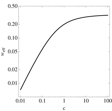
Figure 2: Plot of the equation-of-state parameter $w_{\textrm{eff}}\equiv P_{\rm eff}/\rho_{\rm eff}$ as a function of $c$, within the asymptotically AdS linear dilaton model.

In summary, we find that the asymptotic AdS/linear dilaton background, created by the potential in Eq. (41), gives rise to a cosmological brane-world in which the behavior of the “holographic” effective energy density can range from dark radiation to dark matter, as controlled by the $c$ parameter.

VI Discussion

We now discuss a few conceptual points and relations to the literature.

Birth of the bulk black hole.

In a typical cosmological scenario, analogously to the AdS brane-world, the bulk horizon is created by energy leaked from the brane into the continuum of bulk gravitons and other bulk fields. See Hebecker and March-Russell (2001); Langlois et al. (2002); Langlois and Sorbo (2003) for a consistent analysis in AdS, and Fichet (2022) for the rate in arbitrary background. The radiation feeds the bulk black hole, which typically grows with time. This feeding mechanism is efficient at early times while at late times, the radiation is negligible hence the horizon does not evolve anymore. This corresponds to the low-energy regime in our analysis. The process of dumping energy into the bulk, known since Gubser (2001), is either similar or truely equivalent (via AdS/CFT) to the process of heating up a CFT sector (see e.g. Gubser (2001); Hebecker and March-Russell (2001); von Harling and McDonald (2012, 2012); Brax et al. (2019); Hong et al. (2020)).

What is the dark matter made of?

The dark matter arising in our linear dilaton brane-world is purely made of the curvature of spacetime. However this curvature is the result of populating the bulk with gravitons. Deep in the bulk these gravitons are strongly interacting, and their net effect is the presence of the bulk horizon, which is seen by the brane observer. Since the continuum of gravitons is involved, our result shares, in a sense, some similarity with the proposal of “continuum dark matter” made in Csáki et al. (2022a, b); Csaki et al. (2022). It is plausible that our analysis provides the consistent framework needed to understand cosmology in such models.

VII Prospects

Overall, the results reported in this letter hint at an alternative view of dark matter which certainly deserves further investigation. We thus end with a discussion of future directions.

Cosmological perturbations.

The key calculation presented in this letter shows that the linear dilaton background could explain dark matter in the homogeneous universe. Computing perturbations and structure formation is a task beyond the present work, however the roadmap is clear: the study of cosmological perturbations in our model belongs to the realm of the fluid/gravity correspondence Bhattacharyya et al. (2008); Hubeny et al. (2012). The dark matter of our brane-world model amounts to a (non-conformal) “holographic fluid”, whose properties such as viscosities need to be carefully computed and compared to observations.

Dark matter at galactic scales.

Our brane-world model may explain dark matter at cosmological scale, however nothing is said about galactic scales. To understand how the dark matter emerging in our model behaves at galactic scales we would have to compute less symmetric solutions of the 5D scalar-gravity system, as needed to describe e.g. halos. One should thus investigate $SO(3)$-symmetric solutions, possibly assisted by matter sources on the brane. This is left for future investigation.

Dark matter decay.

In analogy with AdS, the bulk black hole may in principle be able to decay via Hawking radiation into the brane, see Rocha (2008, 2009) for an analysis in AdS. Since the bulk black hole is the origin of dark matter, Hawking decay amounts in our model to “dark matter decay”. It would be very interesting to study this mechanism and its observational consequences, as well as its implications for holography. We leave it as an open question to investigate.

Continuum signatures.

In our model the graviton is accompanied by a gapped continuum that can be experimentally tested, as exemplified by the correction to the Newtonian potential Eq. (32). Standard Model fields can be included in the model by introducing 5D bulk fields and identifying the brane-localized modes as the Standard Model fields. Analogously to the graviton, each Standard Model field is accompanied with a gapped continuum which has generally mild coupling to the brane. Such a setup looks typically like a dark sector Brax et al. (2019). The phenomenology of continuum sectors is an active topic of investigation, see e.g. Katz et al. (2016); Csáki et al. (2019); Lee (2018); Gao et al. (2020); Fichet (2020); Costantino et al. (2020); Chaffey et al. (2021); Csáki et al. (2022a, b); Csaki et al. (2022). The present study reinforces the motivation for such models and, in a sense, starts to explore their cosmology.