Improved Laguerre Spectral Methods with Less Round-off Errors and Better Stability

Abstract

Laguerre polynomials are orthogonal polynomials defined on positive half line with respect to weight $e^{-x}$. They have wide applications in scientific and engineering computations. However, the exponential growth of Laguerre polynomials of high degree makes it hard to apply them to complicated systems that need to use large numbers of Laguerre bases. In this paper, we introduce modified three-term recurrence formula to reduce the round-off error and to avoid overflow and underflow issues in generating generalized Laguerre polynomials and Laguerre functions. We apply the improved Laguerre methods to solve an elliptic equation defined on the half line. More than one thousand Laguerre bases are used in this application and meanwhile accuracy close to machine precision is achieved. The optimal scaling factor of Laguerre methods are studied and found to be independent of number of quadrature points in two cases that Laguerre methods have better convergence speeds than mapped Jacobi methods.

65N35, 65D32, 65G50, 33F05

1 Introduction

Spectral methods, which use orthogonal polynomials or orthogonal trigonometric polynomials as bases, are a class of powerful methods to solve partial differential equations, especially when high accuracy is desired. For problems defined on half line $[0,+\infty)$, Laguerre polynomials are a natural choice, since they are orthogonal polynomials defined on half line with respect to weight $e^{-x}$. However, when apply Laguerre (resp. Hermite) polynomials to solve differential equations defined on half line (resp. whole line), there are several challenges [13, 10, 23]:

1. Computations with Laguerre or Hermite polynomials usually lead to ill-conditioned algorithms and undesired round-off error instabilities.

2. Direct using Laguerre or Hermite polynomials to approximate functions only provide meaningful results inside small intervals since the error estimation is obtained in weighted Sobolev spaces with fast decaying weights

3. Standard Laguerre and Hermite polynomials have poor resolution properties when compared with other types of orthogonal polynomials.

All these challenges have been studied and partially solved. For the first challenge, scaled Laguerre functions are introduced by Funaro[10]. For the second challenge, it is proposed by Shen [23] to use Laguerre functions as bases to form Laguerre spectral methods, this approach also (partially) avoids the first challenge. For the third challenge, it is found that the approximation by Hermite and Laguerre polynomials/functions can be significantly improved by choosing good scaling factors [29, 23]. Due to these pioneering works, the stability and efficiency of Laguerre and Hermite spectral methods are significant improved. They are widely used in scientific and engineering applications. E.g. a stable Laguerre method is applied to solve nonlinear partial differential equations on a semi-infinite interval [16]. Laguerre polynomials/functions are used to form composite spectral or spectral element methods for problems in unbounded domains [15, 33, 25, 31, 2, 8, 27]. Laguerre methods have also been used to construct spectral numerical integrator for ordinary differential equations [14, 17]. Efficient time-splitting Laguerre-Hermite spectral methods are designed for Bose-Einstein condensates [3, 4]. Laguerre and Hermite methods have also been used in optimal control problem [21] and fractional differential equations [5, 9, 30]. Scaling factors in different situations are further investigated [20, 32]. A Laguerre method with scaling factor built in the Laguerre bases is designed and implemented with diagonalization technique [18, 19, 34].

Despite these advances in Laguerre spectral methods for unbounded domains, the existing applications only used small numbers of Laguerre bases. This is partially due to the fact that standard subroutines to generate Laguerre polynomials and Laguerre functions suffer from overflow and underflow issues in generating large numbers of Laguerre-Gauss quadrature points. In this paper we introduce a simple but effective method to handle the underflow problem in calculating the values of Laguerre functions on large Gauss points. Numerical results show our method has better accuracy than existing methods given in  [10, 23]. On the same time, we find that the standard three-term recurrence formula to generate Laguerre polynomials and Laguerre functions leads to serious round-off errors for small arguments close to $0$. We introduce a modified three-term recurrence formula to reduce the round-off error. Numerical results show that the modified recurrence formula improve the accuracy of generating Laguerre polynomials by 2 to 4 decimal digits for small arguments close to 0, comparing to the standard recurrence formula. By using these improved basic algorithms for Laguerre spectral methods, we are able to solve a model elliptic equation defined on semi-infinite interval using more than one thousands Laguerre bases without convergence deterioration. To the best of our knowledge, these is the largest degree of Laguerre bases being used in Laguerre spectral methods. We also study the scaling factor of Laguerre spectral methods, it is found that for the two special cases that Laguerre methods convergent faster than mapped Jacobi methods, the optimal scaling factor is independent of number of Laguerre bases used. This means one can tune the scaling factor on coarse grids and use the optimal value on finer grids. We expect the improved basic algorithms for Laguerre methods and the findings on the optimal scaling factor will accelerate the development and applications of Laguerre spectral methods to large complex systems.

The remain part of this paper is organized as follows. In Section 2, we review some basic properties of generalized Laguerre polynomials/functions and related basic algorithms. In Section 3, we introduce the improved three-term recurrence formula with less round-off error for generalized Laguerre polynomials and functions, and the modified algorithm for generalized Laguerre functions to handle the underflow issue. An error estimation of the three-term recurrence formula is given. In Section 4, application of Laguerre spectral method to a model elliptic equation on semi-infinite interval is presented and the scaling factor is studied. A short summary is given in Section 5.

2 Preliminaries

In this section, we review some basic properties of generalized Laguerre polynomials and functions, which are related to basic algorithms of Laguerre spectral methods. They can be found in standard reference books, e.g. [1, 28, 22, 7, 24].

2.1 Generalized Laguerre polynomials

Generalized Laguerre polynomials, denoted by $\mathcal{L}_{n}^{(\alpha)}(x)$ with ($\alpha>-1$) , are polynomials defined on the half line $\mathbb{R}_{+}:=(0,+\infty)$ and orthogonal with respective to weight

(1) $$\omega_{\alpha}(x)=x^{\alpha}e^{-x},$$

i.e.

(2) $$\int_{0}^{+\infty}\mathcal{L}_{n}^{(\alpha)}(x)\mathcal{L}_{m}^{(\alpha)}(x)\omega_{\alpha}(x)\mathrm{d}x=\gamma_{n}^{(\alpha)}\delta_{nm},$$

where $\delta_{nm}$ is the Kronecker delta symbol and

(3) $$\gamma_{n}^{(\alpha)}=\frac{\Gamma(n+\alpha+1)}{n!}.$$

In particular, $\mathcal{L}_{n}^{(0)}(x)$ is the usual Laguerre polynomials, which will be denoted by $\mathcal{L}_{n}(x)$, its weight $\omega_{0}(x)$ will be denoted by $\omega(x):=e^{-x}$. We also have $\gamma_{n}^{0}=1$, i.e. $\mathcal{L}_{n}(x)$ are normalized orthogonal bases in $L^{2}_{\omega}(\mathbb{R}_{+})$.

In addition to the orthogonality (2), the following formulas provide basic properties and algorithms of Laguerre polynomials.

1. Three-term recurrence formula

   (4) $$\left\{\begin{array}[]{l}\mathcal{L}^{(\alpha)}_{0}(x)=1,\qquad\mathcal{L}^{(\alpha)}_{1}(x)=-x+\alpha+1,\\ (n+1)\mathcal{L}_{n+1}^{(\alpha)}(x)=(2n+\alpha+1-x)\mathcal{L}_{n}^{(\alpha)}(x)-(n+\alpha)\mathcal{L}_{n-1}^{(\alpha)}(x),\quad n\geq 1.\end{array}\right.$$

   From the recurrence formula, we obtain that

   (5) $$\mathcal{L}^{(\alpha)}_{n}(0)=\frac{\Gamma(n+\alpha+1)}{n!\Gamma(\alpha+1)}=\frac{\gamma_{n}^{(\alpha)}}{\Gamma(\alpha+1)}.$$

   In particular, $\mathcal{L}_{n}(0)=1$, $\mathcal{L}_{n}^{(1)}(0)=n+1$.

2. Some formulas related to the derivative of generalized Laguerre polynomials

   (6) $$\partial_{x}\mathcal{L}^{(\alpha)}_{n}(x)=-\mathcal{L}^{(\alpha+1)}_{n-1}(x)=-\sum_{k=0}^{n-1}\mathcal{L}^{(\alpha)}_{k}(x),$$

   (7) $$\partial_{x}\mathcal{L}^{(\alpha)}_{n+1}(x)=\partial_{x}\mathcal{L}^{(\alpha)}_{n}(x)-\mathcal{L}^{(\alpha)}_{n}(x).$$

3. The scaling of Laguerre polynomials is given by Theorem 8.22.5 of [28].

   (8) $$\mathcal{L}^{(\alpha)}_{n}(x)=\frac{1}{\sqrt{\pi}}e^{\frac{x}{2}}x^{-\frac{\alpha}{2}-\frac{1}{4}}n^{\frac{\alpha}{2}-\frac{1}{4}}\times\Bigl{[}\cos\bigl{(}2\sqrt{nx}-\frac{(2\alpha+1)\pi}{4}\bigr{)}+\frac{O(1)}{\sqrt{nx}}\Bigr{]},$$

   for $x\in[c/n,b]$ with $c$ and $b$ being fixed positive numbers. The exponential growth of Laguerre polynomials cause numerical issue in standard (IEEE 754) floating-point arithmetic systems.

2.2 Generalized Laguerre functions

Due to the exponential growth of the generalized Laguerre polynomials, the values $\mathcal{L}^{(\alpha)}_{N}(x)$ at Gauss quadrature points will exceed the representation limit of IEEE 754 standard for double precision floating-point data with $N$ larger than several hundreds, thus cause overflow issue. To remove this limitation, generalized Laguerre functions are considered, which are defined as

(9) $$\widehat{\mathcal{L}}^{(\alpha)}_{n}(x):=e^{-x/2}\mathcal{L}^{(\alpha)}_{n}(x),\quad x\in\mathbb{R}_{+},\quad\alpha>-1.$$

They are orthogonal with respective to weight

(10) $$\hat{\omega}_{\alpha}(x)=x^{\alpha}.$$

The corresponding formulas to generate generalized Laguerre functions and their derivatives are given below.

1. Three-term recurrence formula:

   (11) $$\left\{\displaystyle\begin{array}[]{l}\widehat{\mathcal{L}}^{(\alpha)}_{0}(x)=e^{-x/2},\qquad\widehat{\mathcal{L}}^{(\alpha)}_{1}(x)=(\alpha+1-x)e^{-x/2},\\ (n+1)\widehat{\mathcal{L}}^{(\alpha)}_{n+1}(x)=(2n+\alpha+1-x)\widehat{\mathcal{L}}^{(\alpha)}_{n}(x)-(n+\alpha)\widehat{\mathcal{L}}^{(\alpha)}_{n-1}(x),\quad n\geq 1.\end{array}\right.$$

2. The recurrence formula for derivatives:

   (12) $$\begin{cases}\displaystyle\partial_{x}\widehat{\mathcal{L}}^{(\alpha)}_{0}(x)=-\frac{1}{2}e^{-x/2},\qquad\partial_{x}\widehat{\mathcal{L}}^{(\alpha)}_{1}(x)=-\frac{\alpha+3-x}{2}e^{-x/2},&\\ \displaystyle\partial_{x}\widehat{\mathcal{L}}^{(\alpha)}_{n+1}(x)=\partial_{x}\widehat{\mathcal{L}}^{(\alpha)}_{n}(x)-\frac{1}{2}\widehat{\mathcal{L}}^{(\alpha)}_{n}(x)-\frac{1}{2}\widehat{\mathcal{L}}^{(\alpha)}_{n+1}(x),&n\geq 1.\end{cases}$$

2.3 Laguerre-Gauss type quadrature

Let $\bigl{\{}x_{j}^{(\alpha)},\,\omega_{j}^{(\alpha)}\bigr{\}}_{j=0}^{N}$ be the set of Laguerre-Gauss or Laguerre-Gauss-Radau quadrature nodes and weights.

• For the Laguerre-Gauss quadrature,

  (13) $$\left\{\begin{array}[]{l}\bigl{\{}x_{j}^{(\alpha)}\bigr{\}}_{j=0}^{N}\text{ are the zeros of }\mathcal{L}^{(\alpha)}_{N+1}(x),\text{ and}\\ \displaystyle\omega_{j}^{(\alpha)}=\frac{\Gamma(N+\alpha+1)}{(N+\alpha+1)(N+1)!}\frac{x_{j}^{(\alpha)}}{\bigl{[}\mathcal{L}^{(\alpha)}_{N}(x_{j}^{(\alpha)})\bigr{]}^{2}},\quad 0\leq j\leq N.\end{array}\right.$$

• For the Laguerre-Gauss-Radau quadrature

  (14) $$\left\{\begin{array}[]{l}\displaystyle x_{0}^{(\alpha)}=0,\quad\bigl{\{}x_{j}^{(\alpha)}\bigr{\}}_{j=1}^{N}\text{ are the zeros of }\partial_{x}\mathcal{L}^{(\alpha)}_{N+1}(x),\text{ and}\\[6.0pt] \displaystyle\omega_{0}^{(\alpha)}=\frac{(\alpha+1)\Gamma^{2}(\alpha+1)N!}{\Gamma(N+\alpha+2)},\\[9.0pt] \displaystyle\omega_{j}^{(\alpha)}=\frac{\Gamma(N+\alpha+1)}{N!(N+\alpha+1)}\frac{1}{[\mathcal{L}_{N}^{(\alpha)}(x_{j}^{(\alpha)})]^{2}},\quad 1\leq j\leq N.\end{array}\right.$$

With above nodes and weights, we have

$$\int_{0}^{\infty}p(x)x^{\alpha}e^{-x}\mathrm{d}x=\sum_{j=0}^{N}p(x_{j}^{(\alpha)})\omega_{j}^{(\alpha)},\quad\forall\,p\in P_{2N+\delta},$$

where $\delta=1,0$ for the Laguerre-Gauss quadrature and the Laguerre-Gauss-Radau quadrature, respectively.

To form the Laguerre-Gauss and Laguerre-Gauss-Radau quadrature scheme, we need find the zeros of the Laguerre polynomials, which can be obtained by calculating all eigenvalues of a banded matrix (see e.g. [12][11]). More precisely, by the three-term recurrence formula (4), the zeros $\{x_{j}^{(\alpha)}\}_{j=0}^{N}$ of $\mathcal{L}^{(\alpha)}_{N+1}(x)$ are the eigenvalues of the symmetric tridiagonal matrix (see e.g. [24]):

(15) $$A_{N+1}=\left[\begin{array}[]{ccccc}a_{0}&-\sqrt{b_{1}}&&&\\ -\sqrt{b_{1}}&a_{1}&-\sqrt{b_{2}}&&\\ &\vdots&\vdots&\vdots&\\ &&-\sqrt{b_{N-1}}&a_{N-1}&-\sqrt{b_{N}}\\ &&&-\sqrt{b_{N}}&a_{N}\end{array}\right],$$

where $a_{j}=2j+\alpha+1$, $0\leq j\leq N$, $b_{j}=j(j+\alpha)$, $1\leq j\leq N$. The approach of using this property to calculate the zeros of orthogonal polynomials is referred to as the eigenvalue method.

For small values of $x_{j}^{(\alpha)}$, we have following asymptotic formula

(16) $$\sqrt{x_{j}^{(\alpha)}}=\frac{(j+1)\pi+O(1)}{2\sqrt{N+1}},\quad\text{for}\ x_{j}^{(\alpha)}\in(0,\eta),\ \alpha>-1,$$

where $\eta>0$ is a fixed constant. For the largest point

(17) $$x_{N}^{(\alpha)}=4N+2\alpha+6+O(N^{1/3}).$$

By (6.31.13) of Szegö (1975), we have also for $\alpha=0$

(18) $$x_{j}=C_{j,N}\frac{(j+2)^{2}}{N+2},\quad 0\leq j\leq N,\quad\frac{1}{4}<C_{j,N}<4.$$

By the scaling (17), (8), and the formula (13) and (14), one easily see that the Laguerre-Gauss and Laguerre-Gauss-Radau quadrature weights decay exponentially for large $N$. E.g. the last weights for the 5 -point and 10-point Laguerre-Gauss formula are about $2.337\times 10^{-5}$, $9.912\times 10^{-13}$, respectively [22], and it is $6.770\times 10^{-23}$ for 16-point formula [24]. The unbalanced quadrature weights is not a good property for numerical computations. Fortunately, the Laguerre-Gauss quadrature can be directly extended to the Laguerre function approach, for which we define

(19) $$\hat{\omega}_{j}^{(\alpha)}:=e^{x_{j}^{(\alpha)}}\omega_{j}^{(\alpha)},\quad 0\leq j\leq N.$$

Then

(20) $$\int_{0}^{\infty}p(x)q(x)x^{\alpha}\mathrm{d}x=\sum_{j=0}^{N}p(x_{j}^{(\alpha)})q(x_{j}^{(\alpha)})\hat{\omega}_{j}^{(\alpha)},\quad\forall\,p\in\widehat{P}_{K},\ q\in\widehat{P}_{L},\;K+L\leq 2N+\delta,$$

where

(21) $$\widehat{P}_{N}:=\bigl{\{}\phi:\phi=e^{-x/2}\psi,\quad\forall\,\psi\in P_{N}\bigr{\}},$$

and $\delta=1,0$ for the modified Laguerre-Gauss rule and the modified Laguerre-Gauss-Radau rule, respectively.

3 Improved Laguerre algorithms with less round-off error and better stability

To implement a basic spectral method for solving differential equations, we need basic quadrature and spectral transform algorithms, in which we need first calculate the quadrature points and weights. The quadrature points can be generated by using the eigenvalue method. After accurate quadrature points are obtained, the quadrature weights can be obtained by using formula (13), (14) and (19), in which one needs to evaluate the generalized Laguerre polynomials/functions at Gauss quadrature points.

3.1 Generating Gauss quadrature points

We first use eigenvalue method to generate the Laguerre-Gauss quadrature points. Numerical results show that the eigenvalue method can’t obtain full accuracy using floating-point arithmetic. Usually several significant digits are lost (see the left plot in Figure 1). We then use the following Newton’s iterations to improve the accuracy of quadrature points

(22) $$x_{j}^{n+1}=x_{j}^{n}-\frac{\mathcal{L}^{(\alpha)}_{N}(x_{j}^{n})}{\partial_{x}\mathcal{L}^{(\alpha)}_{N}(x_{j}^{n})},\quad n=0,1,\ldots.$$

To this end, we need a stable subroutine to calculate $\mathcal{L}^{(\alpha)}_{N}(x_{j})$ and $\partial_{x}\mathcal{L}^{(\alpha)}_{N}(x_{j})$ with high accuracy. To evaluate the accuracy of the eigenvalue method and the classical three-term recurrence formula to generate $\mathcal{L}^{(\alpha)}_{N}(x)$ and $\partial_{x}\mathcal{L}^{(\alpha)}_{N}(x)$, we need a method to generate exact (reference) solution, for which we use multiple precision arithmetic (e.g. mpmath in Python or variable precision arithmetic (vpa) in Matlab and Octave) to generate $\mathcal{L}^{(\alpha)}_{N}(x)$ and $\partial_{x}\mathcal{L}^{(\alpha)}_{N}(x)$, and use them to refine the Gauss quadrature points via (22) to generate exact solutions. The results are given in the left plot of Figure 1, from which we see a clear improvement of using Newton’s iterations, especially for large $x_{j}$’s, where the accuracy are improved more than 10 times and double precision limit is reached. However, the improvements for small $x_{j}$’s are not significant. The results for generating Laguerre-Gauss-Radau points are similar, to save space they are not shown in the figure.

Theoretically, if $\mathcal{L}^{(\alpha)}_{N}(x)$ and $\partial_{x}\mathcal{L}^{(\alpha)}_{N}(x)$ are evaluated accurately, the refinement of Gauss points using Newton’s iterations should be able to reach machine accuracy. We think the big numerical errors for $x_{j}$’s close to 0 is mainly caused by the round-off error of the coefficient $2n+\alpha+1-x$ in the three-term recurrence formula (4). Since $x$ is small, but $2n+\alpha+1$ is not small, so some significant digits in $x$ will be lost if we use floating-point system to store $2n+\alpha+1-x$.

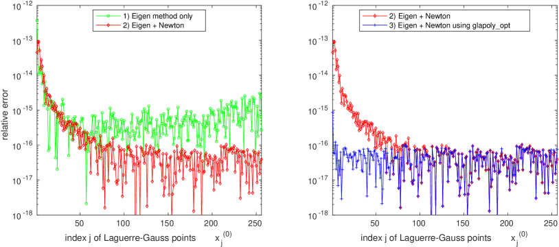
Figure 1: The relative errors of Laguerre-Gauss quadrature points ($N=256$, $\alpha=0$) calculated by different methods. In the right plot, glapoly_opt stands for generalized Laguerre polynomials generated using new approach (23).

3.2 Modified three-term recurrence algorithm

To improve the accuracy of the three-term recurrence algorithm for small values of $x$, we take a new approach, by introducing

$$\delta\mathcal{L}^{(\alpha)}_{n}=\mathcal{L}^{(\alpha)}_{n}-\mathcal{L}^{(\alpha)}_{n-1},\quad n\geq 1.$$

The new recurrence formula is given by

(23) $$\left\{\begin{array}[]{ll}\displaystyle\mathcal{L}^{(\alpha)}_{0}(x)=1,\qquad\mathcal{L}^{(\alpha)}_{1}(x)=1+\alpha-x,&\delta\mathcal{L}^{(\alpha)}_{1}=\alpha-x,\\[3.0pt] \displaystyle\delta\mathcal{L}^{(\alpha)}_{n+1}(x)=\frac{n+\alpha}{n+1}\delta\mathcal{L}^{(\alpha)}_{n}(x)-\frac{x}{n+1}\mathcal{L}^{(\alpha)}_{n}(x),&n\geq 1,\\[6.0pt] \displaystyle\mathcal{L}^{(\alpha)}_{n+1}(x)=\mathcal{L}^{(\alpha)}_{n}(x)+\delta\mathcal{L}^{(\alpha)}_{n+1}(x),&n\geq 1.\end{array}\right.$$

If required, the derivatives $\partial_{x}\mathcal{L}^{(\alpha)}_{n+1}(x)$ is calculated by using (7) when $\mathcal{L}^{(\alpha)}_{n+1}(x)$ is obtained.

Numerical results of generated Laguerre-Gauss points $x_{j}^{(\alpha)}$ for $\alpha=0$, $N=256$ by using the standard and new three-term recurrence formulas are shown in the right plot of Figure 1, from which we see that the new approach perform significantly better than the old standard approach. The only point with relative error larger than machine accuracy is the first quadrature point next to 0. But it still has an improvement of 2 significant digits over the standard recurrence formula with Newton’s iterations.

We then test the error of classical procedures to evaluate Laguerre polynomials at given Gauss points, which are used in the formulas of Gauss quadrature weights (13) and (14). The results of using two methods to generate $\mathcal{L}^{(\alpha)}_{N-1}(x_{j}^{(\alpha)}),j=1,\ldots,N$ for $\alpha=0,N=100$ are presented in the left plot of Figure 2, where glapoly stands for the standard three-term recurrence algorithm, glapoly_vpa24 stands for results generated by standard three-term recurrence algorithm using 24-digit floating-point arithmetic, glapoly_opt stands for the results using new recurrence formula (23). We observe that the classical three-term recurrence algorithm is not very accurate, several significant digits are lost especially for small $x_{j}$’s. On the other hand, glapoly_opt gives much accurate results, especially for smaller $x_{j}$’s.

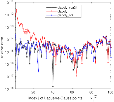
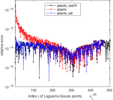
Figure 2: $\mathcal{L}^{(\alpha)}_{N-1}(x_{j}^{(\alpha)})$ for $\alpha=0$ calculated by two methods: glapoly() stands for the traditional formula (4), glapoly_opt stands for the new approach (23), glapoly_vpa24 is a reference solution obtained by using variable-precision algorithms of 24 digits. Left: $N=100$; Right: $N=500$. For glapoly and glapoly_opt in the right plot, the last 37 values are NaN and not plotted.

We next test the results of generating Laguerre polynomials for a larger $N$. In the right plot of Figure 2, we present the results of generating $\mathcal{L}^{(\alpha)}_{N-1}$ at $N$ Laguerre-Gauss points using different methods with $N=500$. We find that with data stored in double precision, the Laguerre polynomial $\mathcal{L}^{(\alpha)}_{499}(x_{j}^{(\alpha)})$ exceeds the representing region of double-precision for $j>463$. We tested that using double-precision floating-point number system to obtain (13) with $a=0,1,2,3,4,5,6$, the maximum Laguerre-Gauss quadrature scheme can be generated is $N=362$. We will propose a method to overcome the overflow problem later in this section, but in next subsection, we first give an error estimate of the three-term recurrence formulas.

3.3 An error estimate for the three-term recurrence algorithms

For three-term recurrence formula (4), we have

$$\mathcal{L}_{n+1}^{(\alpha)}(1+\delta_{n+1})=\frac{2n+\alpha+1-x(1+\eta_{x})}{n+1}(1+\eta^{a}_{n})\mathcal{L}_{n}^{(\alpha)}(1+\delta_{n})-\frac{n+\alpha}{n+1}(1+\eta^{b}_{n})\mathcal{L}_{n-1}^{(\alpha)}(1+\delta_{n-1}),$$

where $\eta_{x},\eta^{a}_{n},\eta_{n}^{b}$ account for the relative round-off errors of the corresponding coefficients, $\delta_{n+1},\delta_{n}$, $\delta_{n-1}$ are the relative errors of $\mathcal{L}^{(\alpha)}_{n+1}$, $\mathcal{L}^{(\alpha)}_{n}$, $\mathcal{L}^{(\alpha)}_{n-1}$, respectively. Using notation $e_{n}=\mathcal{L}^{(\alpha)}_{n}(x)\delta_{n}$, we have

$$e_{n+1} = \frac{2n+\alpha+1-x(1+\eta_{x})}{n+1}(1+\eta^{a}_{n})(\mathcal{L}_{n}^{(\alpha)}+e_{n})-\frac{n+\alpha}{n+1}(1+\eta^{b}_{n})(\mathcal{L}_{n-1}^{(\alpha)}+e_{n-1})$$

$$-\frac{2n+\alpha+1-x}{n+1}\mathcal{L}^{(\alpha)}_{n}+\frac{n+\alpha}{n+1}\mathcal{L}^{(\alpha)}_{n-1}$$

$$= -\frac{x}{n+1}\eta_{x}(1+\eta^{a}_{n})(\mathcal{L}_{n}^{(\alpha)}+e_{n})+\frac{2n+\alpha+1-x}{n+1}\eta^{a}_{n}(\mathcal{L}_{n}^{(\alpha)}+e_{n})+\frac{2n+\alpha+1-x}{n+1}e_{n}$$

$$-\frac{n+\alpha}{n+1}\eta^{b}_{n}(\mathcal{L}_{n-1}^{(\alpha)}+e_{n-1})-\frac{n+\alpha}{n+1}e_{n-1}$$

$$= -\frac{x}{n+1}\mathcal{L}_{n}^{(\alpha)}\eta_{x}+\frac{2n+\alpha+1-x}{n+1}\mathcal{L}_{n}^{(\alpha)}\eta^{a}_{n}+\frac{2n+\alpha+1-x}{n+1}e_{n}$$

$$-\frac{n+\alpha}{n+1}\mathcal{L}_{n-1}^{(\alpha)}\eta^{b}_{n}-\frac{n+\alpha}{n+1}e_{n-1}+\xi_{n},$$

where $\xi_{n}$ includes high-order error terms, which can be bounded by $\varepsilon(4|e_{n}|+|e_{n-1}|)$. Here $\varepsilon$ is the bound of relative round-off error of the floating-point system used. For double precision data in IEEE 754 standard, $\varepsilon\approx 2.22\times 10^{-16}$. The above result can be written as

(24) $$\left\{\begin{array}[]{l}e_{n+1}=\frac{2n+\alpha+1-x}{n+1}e_{n}-\frac{n+\alpha}{n+1}e_{n-1}+\zeta_{n},\quad n\geq 1,\\ e_{0}=0,\\ e_{1}=\mathcal{L}_{1}^{(\alpha)}\eta_{0}^{a},\quad|\eta_{0}^{a}|\sim\varepsilon.\end{array}\right.$$

where

(25) $$\zeta_{n}=\xi_{n}-\frac{x}{n+1}\mathcal{L}_{n}^{(\alpha)}\eta_{x}+\frac{2n+\alpha+1-x}{n+1}\mathcal{L}_{n}^{(\alpha)}\eta^{a}_{n}-\frac{n+\alpha}{n+1}\mathcal{L}_{n-1}^{(\alpha)}\eta^{b}_{n}.$$

For $x\ll 1$, $n\gg 1$, $\zeta_{n}\sim\Bigl{(}2+\dfrac{x}{n+1}\Bigr{)}|\mathcal{L}_{n}^{(\alpha)}|\varepsilon+|\mathcal{L}_{n-1}^{(\alpha)}|\varepsilon$.

Assume that $\alpha>-1$, Then, for any $\eta>0$ with $3-\alpha-x-\eta>0$ , the error propagation given by (24) satisfies the following estimate:

$$E_{n+1}\leq\left\{\begin{array}[]{ll}E_{1}+\frac{(n+1)(n+2)(2n+3)}{6\eta}\max_{s}\zeta_{s}^{2},&\text{if}\ 1-2\alpha-x-\eta\geq 0,\\ \beta_{n}E_{1}+\frac{(n-3)(n+1)^{2}+29\beta_{n}}{\eta}\max_{s}\zeta_{s}^{2},&\text{if}\ -1.5<1-2\alpha-x-\eta<0\ \text{and}\ \alpha\geq 0,\end{array}\right.$$

for $n\geq 1$, where $E_{n}:=xe_{n}^{2}+(n+\alpha)(e_{n}-e_{n-1})^{2}$ and $\beta_{n}=\frac{\Gamma(n+2+\alpha)/\Gamma(2+\alpha)}{\Gamma(n+3-\alpha-x-\eta)/\Gamma(3-\alpha-x-\eta)}$.

Proof.

We first rewrite the first equation of (24) as

$$(e_{n+1}-e_{n})-\frac{n+\alpha}{n+1}(e_{n}-e_{n-1})=-\frac{x}{n+1}e_{n}+\zeta_{n}.$$

Then multiply $d_{n+1}:=e_{n+1}-e_{n}$ on both sides, we obtain

$$\frac{1-\alpha}{n+1}d_{n+1}^{2}+\frac{1}{2}\frac{n+\alpha}{n+1}[d_{n+1}^{2}-d_{n}^{2}+(d_{n+1}-d_{n})^{2}]=\frac{1}{2}\frac{x}{n+1}[e_{n}^{2}-e_{n+1}^{2}+d_{n+1}^{2}]+\zeta_{n}d_{n+1},$$

i.e.

$$\frac{x}{n+1}[e_{n+1}^{2}-e_{n}^{2}]+\frac{n+2-\alpha-x}{n+1}d_{n+1}^{2}-\frac{n+\alpha}{n+1}d_{n}^{2}+\frac{n+\alpha}{n+1}(d_{n+1}-d_{n})^{2}=2\zeta_{n}d_{n+1},$$

or

$$xe_{n+1}^{2}+(n+2-\alpha-x)d_{n+1}^{2}+(n+\alpha)(d_{n+1}-d_{n})^{2}=xe_{n}^{2}+(n+\alpha)d_{n}^{2}+2(n+1)\zeta_{n}d_{n+1}.$$

Then, by using Cauchy inequality with $\eta$ on $\zeta_{n}d_{n+1}$: $2\zeta_{n}d_{n+1}\leq\frac{n+1}{\eta}\zeta_{n}^{2}+\frac{\eta}{n+1}d_{n+1}^{2}$, we get

(26) $$xe_{n+1}^{2}+(n+2-\alpha-x-\eta)d_{n+1}^{2}+(n+\alpha)(d_{n+1}-d_{n})^{2}\leq xe_{n}^{2}+(n+\alpha)d_{n}^{2}+\frac{(n+1)^{2}}{\eta}\zeta_{n}^{2}.$$

Define

$$r_{n}:=\max\left\{1,\frac{n+1+\alpha}{n+2-\alpha-x-\eta}\right\}.$$

Then for $n\geq 1$, $3-\alpha-x-y>0$,

$$E_{n+1}\leq r_{n}E_{n}+r_{n}\frac{(n+1)^{2}}{\eta}\zeta_{n}^{2}.$$

Then by mathematical induction, we obtain

(27) $$E_{n+1}\leq(\Pi_{k=1}^{n}r_{k})E_{1}+\sum_{s=1}^{n}(\Pi_{k=s}^{n}r_{k})\frac{(s+1)^{2}}{\eta}\zeta_{s}^{2},\quad n\geq 1.$$

When $1-2\alpha-x-\eta\geq 0$, we have $r_{n}=1$, thus

(28) $$E_{n+1}\leq E_{1}+\sum_{s=1}^{n}\frac{(s+1)^{2}}{\eta}\zeta_{s}^{2}\leq E_{1}+\frac{(n+1)(n+2)(2n+3)}{6\eta}\max_{s}\zeta_{s}^{2}.$$

When $-1.5<1-2\alpha-x-\eta<0$, $r_{n}=\frac{n+1+\alpha}{n+2-\alpha-x-\eta}>1$. Let $b_{s}=(\Pi_{k=s}^{n}r_{k})\frac{(s+1)^{2}}{\eta}$, then

$$b_{s}/b_{s-1}=\frac{(s+1)^{2}}{s^{2}}\frac{s+1-\alpha-x-\eta}{s+\alpha}=\left(1+\frac{2}{s}+\frac{1}{s^{2}}\right)\left(1-\frac{\beta}{s+\alpha}\right),$$

where $0<\beta=2\alpha+x+\eta-1\leq 1.5$, which means

(29) $$\frac{b_{s}}{b_{s-1}}=1+\frac{(2-\beta)s+2\alpha-2\beta}{s(s+\alpha)}+\frac{1}{s^{2}}\frac{s+\alpha-\beta}{s+\alpha}\geq 1\quad\text{if}\ s\geq 5,\alpha\geq 0.$$

Define $\beta_{n}^{s}=\Pi_{k=s}^{n}r_{k}$, and $\beta_{n}=\beta_{n}^{1}$. From above inequality and (27), we have

$$E_{n+1} \leq\beta_{n}E_{1}+\left(\frac{(n-3)(n+1)^{2}}{\eta}+\sum_{s=1}^{3}\beta_{n}^{s}\frac{(s+1)^{2}}{\eta}\right)\max_{s}\zeta_{s}^{2}$$

(30) $$\leq\beta_{n}E_{1}+\left(\frac{(n-3)(n+1)^{2}}{\eta}+\beta_{n}\frac{29}{\eta}\right)\max_{s}\zeta_{s}^{2}.$$

Combine the two cases (28) and (30), we obtain the desired estimate.

From above theorem, it is easy to deduce the following result.

Theorem 3.1.

For $-1<\alpha\leq 1/4,x<1/4$, taking $\eta=1/4$, we have error estimate for (24):

(31) $$|e_{n+1}| \leq\sqrt{\frac{1}{|x|}\biggl{(}(1+\alpha+x)e_{1}^{2}+\frac{2(n+1)(n+2)(2n+3)}{3}\max_{s}\zeta_{s}^{2}\biggr{)}}$$

(32) $$\leq\left(2+\frac{2(n+2)^{3/2}}{\sqrt{3}}\right)\frac{\max\{|e_{1}|,|\zeta_{s}|\}}{|x|^{1/2}}.$$

For $\alpha\geq 0$, $3-\alpha-x-\eta>0$, $-1.5\leq 1-2\alpha-x-\eta<0$, we have

$$|e_{n+1}| \leq \sqrt{\frac{1}{|x|}\left[\beta_{n}(1+\alpha+x)e_{1}^{2}+\frac{29\beta_{n}+(n-3)(n+1)^{2}}{\eta}\max_{s}\zeta_{s}^{2}\right]}$$

$$\leq \left(2\sqrt{\beta_{n}}+\frac{5.5\sqrt{\beta_{n}}+n^{1/2}(n+1)}{\sqrt{\eta}}\right)\frac{\max\{|e_{1}|,|\zeta_{s}|\}}{|x|^{1/2}},$$

Here $\beta_{n}\sim O((n+1+\alpha)^{2\alpha+x+\eta-1})$. In particular, for $\alpha=1$, $x<1/4$, taking $\eta=1/4$, we have

$$|e_{n+1}|\leq(O(n^{3/4})+O(n^{3/2}))\frac{\max\{|e_{1}|,|\zeta_{s}|\}}{|x|^{1/2}}\sim O(n^{3/2})\frac{\max\{|e_{1}|,|\zeta_{s}|\}}{|x|^{1/2}}.$$

Remark 3.2.

Since $e_{1}\sim|\mathcal{L}_{1}^{(\alpha)}|\varepsilon$, $\zeta_{s}\sim\left(\left(2+\frac{x}{n+1}\right)|\mathcal{L}_{s}^{(\alpha)}|+|\mathcal{L}_{s-1}^{(\alpha)}|\right)\varepsilon$. For $x$ close to the smallest Gauss point, by (16), we have $x\sim O(1/N)$, thus $|e_{N}|\lesssim O(N^{2}|\mathcal{L}_{n}^{(\alpha)}|\varepsilon)$. Note that this is a worst-case error estimate. In practice, the numerical errors will be smaller due to the cancellations in summation of random round-off errors.

For iteration (23), we have

$$\left\{\begin{array}[]{l}\delta\mathcal{L}^{(\alpha)}_{n+1}(x)(1+\delta_{n+1}^{a})=\frac{n+\alpha}{n+1}(1+\eta_{n}^{a})\delta\mathcal{L}^{(\alpha)}_{n}(1+\delta_{n}^{a})-\frac{x}{n+1}(1+\eta_{n}^{b})\mathcal{L}^{(\alpha)}_{n}(x)(1+\delta_{n}^{b}),\\[6.0pt] \mathcal{L}^{(\alpha)}_{n+1}(1+\delta_{n+1}^{b})=\mathcal{L}^{(\alpha)}_{n}(x)(1+\delta_{n}^{b})+\delta\mathcal{L}^{(\alpha)}_{n+1}(x)(1+\delta_{n+1}^{a}).\end{array}\right.$$

From above equation, we obtain error propagation equation

(33) $$\left\{\begin{array}[]{l}d_{n+1}=\frac{n+\alpha}{n+1}d_{n}-\frac{x}{n+1}e_{n}+\zeta_{n}^{\delta},\quad n\geq 1,\\ e_{n+1}=e_{n}+d_{n+1},\quad n\geq 1,\\ e_{0}=0,\quad d_{1}=e_{1}.\end{array}\right.$$

where

(34) $$\zeta_{n}^{\delta}=\frac{n+\alpha}{n+1}\delta\mathcal{L}^{(\alpha)}_{n}\eta_{n}^{a}-\frac{x}{n+1}\mathcal{L}^{(\alpha)}_{n}\eta_{n}^{b}+\xi^{\delta}_{n},\qquad\xi^{\delta}_{n}=\frac{n+\alpha}{n+1}\eta_{n}^{a}d_{n}-\frac{x}{n+1}\eta_{n}^{b}e_{n}.$$

Substituting for $d_{n+1}=e_{n+1}-e_{n}$, and $d_{n}=e_{n}-e_{n-1}$, the first equation in (33) becomes

(35) $$e_{n+1}-e_{n}=\frac{n+\alpha}{n+1}(e_{n}-e_{n-1})-\frac{x}{n+1}e_{n}+\zeta_{n}^{\delta}.$$

We notice that the error equation is equivalent to (24) except the difference in $\zeta_{n}$ and $\zeta_{n}^{\delta}$. From equation (34), we know than $\zeta_{n}^{\delta}\sim O\left(\bigl{|}\delta\mathcal{L}^{(\alpha)}_{n}\bigr{|}+\frac{x}{n+1}\bigl{|}\mathcal{L}^{(\alpha)}_{n}\bigr{|}\right)\varepsilon$. We observe that $\bigl{|}\delta\mathcal{L}^{(\alpha)}_{n}(x)\bigr{|}$ is in general smaller than $\bigl{|}\mathcal{L}^{(\alpha)}_{n}(x)\bigr{|}$ for $x$ small (see Figure 3), thus $\zeta_{n}^{\delta}$ is in general smaller than $\zeta_{n}$ for $x\ll n+1$. So it is expected that the iteration algorithm (23) produce smaller numerical errors than (4) for $x$ not too large, which has been demonstrated in Figure 2.

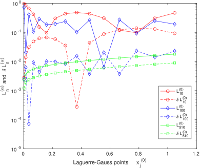
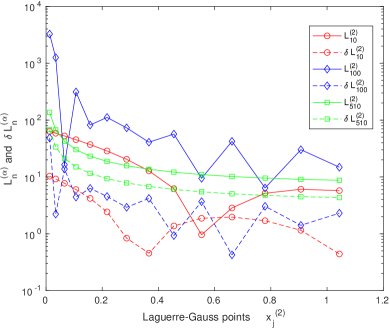
Figure 3: $|\mathcal{L}^{(\alpha)}_{n}(x_{j}^{(\alpha)})|$ and $|\delta\mathcal{L}^{(\alpha)}_{n}(x_{j}^{(\alpha)})|$, $n=10,100,510$, $\alpha=0$ (left) and $\alpha=2$ (right). $x_{j}^{(\alpha)}$ are from 512th order Laguerre-Gauss points.

3.4 Stable algorithms for Laguerre functions and Gauss points

To remove the overflow problem associated with Laguerre polynomials approach, we show how to use the Laguerre function approach to generate corresponding Gauss quadrature scheme.

We first use a procedure similar to (23) to generate generalized Laguerre functions.

(36) $$\left\{\begin{array}[]{ll}\widehat{\mathcal{L}}^{(\alpha)}_{0}(x)=e^{-x/2},\qquad\widehat{\mathcal{L}}^{(\alpha)}_{1}(x)=(1+\alpha-x)e^{-x/2},&\delta\widehat{\mathcal{L}}^{(\alpha)}_{1}=(\alpha-x)e^{-x/2},\\[3.0pt] \displaystyle\delta\widehat{\mathcal{L}}^{(\alpha)}_{n+1}(x)=\frac{n+\alpha}{n+1}\delta\widehat{\mathcal{L}}^{(\alpha)}_{n}(x)-\frac{x}{n+1}\widehat{\mathcal{L}}^{(\alpha)}_{n}(x),&n\geq 1,\\[9.0pt] \widehat{\mathcal{L}}^{(\alpha)}_{n+1}(x)=\widehat{\mathcal{L}}^{(\alpha)}_{n}(x)+\delta\widehat{\mathcal{L}}^{(\alpha)}_{n+1}(x),&n\geq 1.\end{array}\right.$$

The results of calculating $\widehat{\mathcal{L}}^{(\alpha)}_{N-1}(x_{j}^{(\alpha)})$ for $\alpha=0,N=200$ using several methods are presented in the left plot of Figure 4. We see the new recurrence formula (36), which is denoted by glafun_opt, improve the results of standard approach (denoted by glafun) significantly, especially for small quadrature points. It is almost as accurate as the results obtained using 24-digit high-precision arithmetic (denoted by glafun_vpa24), which means the major numerical errors are from the floating-point round-off error of the Gauss points.

However, to generate the Laguerre-Gauss quadrature rule, if we directly multiply the whole weight $e^{-x_{j}^{(\alpha)}/2}$ to the Laguerre polynomials to obtain the corresponding Laguerre functions, we will encounter double precision underflow for $N\geq 383$ when $\alpha=0,1$, since for $x\gtrsim 745$, $e^{-x}$ will be treated as zero in double precision system of IEEE 754 standard.

There are several methods have been proposed to overcome the overflow and underflow problem, e.g. the scaled Laguerre function method proposed by Funaro [10], and the sign and amplitude factor method suggested by Shen [23]. Here, we propose to multiply the weights gradually and adaptively. More precisely, in the iteration procedure, we monitor the magnitude of the iteration variable, if it is larger than a given threshold, then we multiply it by a portion of $e^{-x_{j}^{(\alpha)}/2}$ to make it smaller than another threshold. At the end of the iteration, we apply the remaining parts of the weight to obtain desired results. The overall procedure is given in Algorithm 1.

Algorithm 1 glafun_opt

1:  Input: $N$, $\alpha$, $x$, $K_{1}=32$, $K_{2}=32$

2:  Output: $y=\widehat{\mathcal{L}}^{(\alpha)}_{N}(x)$

3:  if $N=0$ then

4:     set $y=\exp(-x/2)$

5:     return  $y$

6:  end if

7:  if $N=1$ then

8:     set $y=(1+\alpha-x)\exp(-x/2)$

9:     return  $y$

10:  end if

11:  set $L=1+\alpha-x$;

12:  set $\mathrm{d}L=\alpha-x$;

13:  set $x_{b}=x/2$;

14:  for k=1 to $N-1$ do

15:     set $\mathrm{d}L=((k+\alpha)\mathrm{d}L-xL)/(k+1)$;

16:     set $L=L+\mathrm{d}L$;

17:     if $k=1$ or $|L|>\exp(K_{1})$ then

18:        set $x_{c}=\min(\max(\log|L|+K_{2},0),x_{b})$;

19:        set $\mathrm{d}L=\mathrm{d}L\exp(-x_{c})$;

20:        set $L=L\exp(-x_{c})$;

21:        set $x_{b}=x_{b}-x_{c}$;

22:     end if

23:  end for

24:  set $y=L\exp(-x_{b})$;

25:  return  $y$

Note that in the Algorithm 1, $K_{1}$, $K_{2}$ are two given positive constants. We require $K_{1}+K_{2}<80$ to avoid overflow when $x$ and $L$ are stored in single or double precision. In all the numerical experiments presented in this paper, we set $K_{1}=K_{2}=32$. The results of $N=1000$ is given in the right plot of Figure 4.  We see the algorithm glafun_opt is as accurate as the glafun_vpa24 for large $x_{j}$’s, while the standard 3-term recurrence formula is only accurate for $500<j\lesssim 700$, but overflow for large $x_{j}$’s. For small $x_{j}$’s, the results of glafun_opt is slight worse than the glafun_vpa24 results, but still has improvement up to 4 significant digits comparing to the standard glafun method.

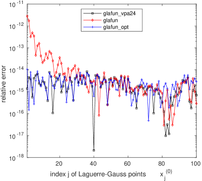
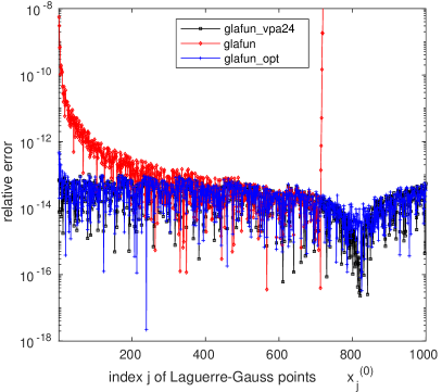
Figure 4: The relative error of $\widehat{\mathcal{L}}^{(\alpha)}_{N-1}(x_{j}^{(\alpha)})$ calculated using different methods. Left: $\alpha=0,N=100$, Right: $\alpha=0,N=1000$.

Before ending this section, we compare the new recurrence algorithm to generate generalized Laguerre functions with the method proposed in [23] and the method proposed in [10]. Note that in [10], scaled Laguerre functions are introduced, which is not equivalent to standard Laguerre functions. But we can obtain standard Laguerre functions by multiplying an appropriate factor on the scaled Laguerre functions. The numerical results are given in Figure 5, from which we see all the three methods can generate generalized Laguerre functions for $N>500$ with reasonable accuracy, but the method proposed here give significantly better results than the other two methods.

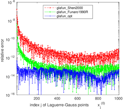
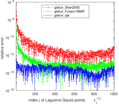
Figure 5: The relative error of $\widehat{\mathcal{L}}^{(\alpha)}_{N-1}(x_{j}^{(\alpha)})$ calculated using different methods. Left: $\alpha=0,N=1000$, Right: $\alpha=1,N=1000$.

4 Application: Laguerre method with best scaling factor

4.1 The Laguerre spectral method for an elliptic equation defined on half line

Consider the following model equation

(37) $$-u_{x\,x}+\gamma u=f,\quad x\in\mathbb{R}_{+},\quad\gamma>0;\quad u(0)=0,\quad\lim_{x\rightarrow+\infty}u(x)=0.$$

The corresponding weak formulation is: find $u\in H_{0}^{1}(\mathbb{R}_{+})$, such that

(38) $$a(u,v):=(u^{\prime},v^{\prime})+\gamma(u,v)=(f,v),\quad\forall\,v\in H_{0}^{1}(\mathbb{R}_{+}),$$

for $f\in H_{0}^{1}(\mathbb{R}_{+})^{\prime}$. Here $H_{0}^{1}(\mathbb{R}_{+})^{\prime}$ is the dual space of $H_{0}^{1}(\mathbb{R}_{+}):=\bigl{\{}v\in H^{1}(\mathbb{R}_{+})\;\text{and}\;v(0)=0\bigr{\}}$.

It is clear than the problem admits a unique solution, since

$$a(u,u)=|u|_{1}^{2}+\gamma\|u\|^{2}\geqslant\min(1,\gamma)\|u\|_{1}^{2},\quad\forall\,u\in H_{0}^{1}(\mathbb{R}_{+}).$$

Define

$$\widehat{P}_{N}^{0}=\operatorname{span}\Set{\psi_{n}(x):=e^{-x/2}\bigl{(}\mathcal{L}^{(0)}_{n}(x)-\mathcal{L}^{(0)}_{n+1}(x)\bigr{)},\>n=0,\ldots,N-1}.$$

The Laguerre spectral-Galerkin approximation to (38) is : Find $u_{N}\in\widehat{P}_{N}^{0}$, such that

(39) $$a(u_{N},v_{N})=(\hat{I}_{M}f,v_{N}),\quad\forall\,v_{N}\in\widehat{P}_{N}^{0}.$$

Here $\hat{I}_{M}$ denotes the interpolation from $C(\mathbb{R}_{+})$ to $\hat{P}_{M}$ using $M+1$ Laguerre-Gauss points.

The error of the above Laguerre-Galerkin method (39) is given by [24]:

Theorem 4.1.

Consider $\alpha=0$,  $\gamma>0$. If $u\in H_{0}^{1}(\mathbb{R}_{+})$, $\hat{\partial}_{x}u:=\left(\partial_{x}+\frac{1}{2}\right)u\in\hat{B}_{0}^{m-1}(\mathbb{R}_{+})$, $f\in C(\bar{\mathbb{R}}_{+})\cap\hat{B}_{0}^{k}(\mathbb{R}_{+})$ and $\hat{\partial}_{x}f\in\hat{B}_{0}^{k-1}(\mathbb{R}_{+})$ with $1\leqslant m\leqslant N+1$, $1\leq k\leq M+1$, then we have

(40) $$\|u-u_{N}\|_{1}\leqslant c\sqrt{\frac{(N-m+1)!}{N!}}\|\hat{\partial}_{x}^{m}u\|_{\hat{\omega}_{m-1}}\\ +c\sqrt{\frac{(M-k+1)!}{M!}}\Bigl{(}\|\hat{\partial}_{x}^{k}f\|_{\hat{\omega}_{k-1}}+(\ln M)^{1/2}\|\hat{\partial}_{x}^{k}f\|_{\hat{\omega}_{k}}\Bigr{)},$$

where $c$ is a positive constant independent of $m,k,N,M,u$ and $f$. Here, the weighted Sobolev space $\hat{B}^{m}_{\alpha}(\mathbb{R}_{+})$ together with its associated norm are defined as

$$\hat{B}_{\alpha}^{m}(\mathbb{R}_{+}):=\Set{u\mid\hat{\partial}_{x}^{k}u\in L_{\hat{\omega}_{\alpha+k}}^{2}(\mathbb{R}_{+}),\;0\leqslant k\leq m},\qquad\|u\|_{\hat{B}_{\alpha}^{m}}:=\biggl{(}\sum_{k=0}^{m}\|\hat{\partial}_{x}^{k}u\|_{\hat{\omega}_{\alpha+k}}^{2}\biggr{)}^{1/2}.$$

We will test the Laguerre method for (37) with exponential and algebraic decay solutions. In particular, we will test three cases with exact solutions given below:

(41) $$u_{1}(x)=\sin(kx)e^{-x},\qquad u_{2}(x)=(1+x)^{-r},\qquad u_{3}(x)=\cos(kx)(1+x)^{-r}.$$

4.2 The scaling factor

It is known that the accuracy of spectral methods for unbounded domain can be improved significantly by using a good scaling factor [6][29][26]. An effective empirical rule is proposed for the Hermite spectral method by Tang [29], where a scaling factor $\beta$ is added to the Hermite function basis $\psi_{k}(\beta x)$, such that the largest Hermite-Gauss quadrature point $\max_{j}|x^{(N)}_{j}|$ after the scaling is located at a given threshold position

(42) $$\max_{j}|x_{j}^{(N)}|/\beta=x_{M},$$

where $x_{M}$ is determined by the criterion that the solution $u(x)$ is numerically neglectable for $|x|>x_{M}$, i.e. for a given tolerance error $\varepsilon$,

$$|u(x)|<\varepsilon,\quad\forall\>|x|\geqslant x_{M}.$$

This approach is very effective and successful. Similar treatments have been applied to Laguerre spectral methods [23][26]. However, by using this approach, one has to determine $x_{M}$, and the choice $\beta$ given by (42) depends on the number of quadrature points used. We found that for special exponential decay functions, e.g. the $u_{1}(x)$ defined in (41), an optimal scaling factor $\beta$ can be determined by a rigorous error estimation. To see this, we first apply the linear transform $y=\beta x$ to equation (37) to get

(43) $$-v_{yy}+\frac{\gamma}{\beta^{2}}v=\frac{1}{\beta^{2}}g(y),\quad v(0)=0,\quad\lim_{y\rightarrow+\infty}v(y)=0,$$

where $v(y)=u(x)=u(y/\beta)$, $g(y)=f(y/\beta)$. It is obvious that for any $u^{\ast}(x)$ satisfies (37), $v^{\ast}(y)=u^{\ast}(y/\beta)$ satisfies (43). The difference is that the convergence speed using $\hat{P}_{N}^{0}$ to approximate problem (37) and (43) are different. By applying (40) to (43), and omitting the interpolation error for simplicity (suppose we choose $M>N$ to make the interpolation error smaller than the projection error), we obtain

(44) $$\|v-v_{N}\|_{1}{\leqslant c_{1}}\sqrt{\frac{(N-m+1)!}{N!}}\|\hat{\partial}_{y}^{m}v\|_{\hat{\omega}_{m-1}}$$

where $c_{1}=c\frac{\max(1,\gamma/\beta^{2})}{\min(1,\gamma/\beta^{2})}$.

Obviously, the convergence speed depends on the choice of measurement. We should measure error using certain norm of $u(x)$. Notice that

$$\|v-v_{N}\|^{2}=\int_{0}^{\infty}|v(y)-v_{N}(y)|^{{}^{2}}\mathrm{d}y=\beta\int_{0}^{\infty}|u(x)-u_{N}(x)|^{2}\mathrm{d}x=\beta\|u-u_{N}\|^{2},$$

$$|v-v_{N}|_{1}^{2}=\int_{0}^{\infty}|\partial_{y}v(y)-\partial_{y}v_{N}(y)|^{{}^{2}}\mathrm{d}y=\frac{1}{\beta}\int_{0}^{\infty}|\partial_{x}u-\partial_{x}u_{N}(x)|^{2}\mathrm{d}x=\frac{1}{\beta}|u-u_{N}|_{1}^{2}.$$

We have

(45) $$|u-u_{N}|_{1}=\sqrt{\beta}|v-v_{N}|_{1}\leqslant c\sqrt{\beta}\frac{\max(1,\gamma/\beta^{2})}{\min(1,\gamma/\beta^{2})}\sqrt{\frac{(N-m+1)!}{N!}}\|\hat{\partial}_{y}^{m}v\|_{\hat{\omega}_{m-1}}$$

(46) $$\|u-u_{N}\|=\frac{1}{\sqrt{\beta}}\|v-v_{N}\|\leq\frac{c}{\sqrt{\beta}}\frac{\max(1,\gamma/\beta^{2})}{\min(1,\gamma/\beta^{2})}\sqrt{\frac{(N-m+1)!}{N!}}\|\hat{\partial}_{y}^{m}v\|_{\hat{\omega}_{m-1}}.$$

The errors depend on $\|\hat{\partial}_{y}^{m}v\|_{\hat{\omega}_{m-1}}$, which is also related to $\beta$, since

(47) $$\|\hat{\partial}_{y}^{m}v\|_{\hat{\omega}_{m-1}}^{2}=\int_{0}^{\infty}|(\partial_{y}+1/2)^{m}u(y/\beta)|^{2}y^{m-1}\mathrm{d}y=\beta^{m}\int_{0}^{\infty}|(\partial_{x}/\beta+1/2)^{m}u(x)|^{2}x^{m-1}\mathrm{d}x.$$

When $\beta\rightarrow 0$, we have

$$\beta^{\pm\frac{1}{2}}\frac{\max(1,\gamma/\beta^{2})}{\min(1,\gamma/\beta^{2})}\rightarrow O\left(\frac{\gamma}{\beta^{2\mp 1/2}}\right),\quad\operatorname{and}\quad\|\hat{\partial}_{y}^{m}v\|_{\hat{\omega}_{m-1}}^{2}\rightarrow\frac{1}{\beta^{m}}\int_{0}^{\infty}|\partial_{x}^{m}u(x)|^{2}x^{m-1}\mathrm{d}x.$$

When $\beta\rightarrow+\infty$, we have

$$\beta^{\pm\frac{1}{2}}\frac{\max(1,\gamma/\beta^{2})}{\min(1,\gamma/\beta^{2})}\rightarrow O\left(\frac{\beta^{2\pm 1/2}}{\gamma}\right),\quad\operatorname{and}\quad\|\hat{\partial}_{y}^{m}v\|_{\hat{\omega}_{m-1}}^{2}\rightarrow\beta^{m}\int_{0}^{\infty}\left|\frac{1}{2^{m}}u(x)\right|^{2}x^{m-1}\mathrm{d}x.$$

So, for $m\geqslant 1$, $\int_{0}^{\infty}\left|\frac{1}{2^{m}}u(x)\right|^{2}x^{m-1}\mathrm{d}x>0$ and $\int_{0}^{\infty}|\partial_{x}^{m}u(x)|^{2}x^{m-1}\mathrm{d}x>0$, the right hand sides of (45) and (46) have unbounded limit at $\beta\rightarrow 0$ and $\beta\rightarrow\infty$. Therefore, there exists an optimal value $\beta$ leads to optimal smallest value of the right hand sides of (45) and (46).

4.2.1 Optimal scaling factor for the exponential decay function

Now, we consider a special case $u(x)=e^{zx},$ where $z\in\mathbb{C}$, $\Re(z)<0$. Then

$$\|\hat{\partial}_{y}^{m}v\|_{\hat{\omega}_{m-1}}^{2} = \beta^{m}\int_{0}^{\infty}|(\partial_{x}/\beta+1/2)^{m}e^{zx}|^{2}x^{m-1}\mathrm{d}x$$

$$= \beta^{m}\int_{0}^{\infty}\bigl{|}(z/\beta+1/2)^{2m}\bigr{|}|e^{2zx}|x^{m-1}\mathrm{d}x$$

$$= \biggl{|}\left(z/\sqrt{\beta}+\sqrt{\beta}/2\right)^{2m}\biggr{|}\int_{0}^{\infty}|e^{2zx}|x^{m-1}\mathrm{d}x$$

$$= \left|z/\sqrt{\beta}+\sqrt{\beta}/2\right|^{2m}\frac{(m-1)!}{\Re(2z)^{m}}$$

To make $\|\hat{\partial}_{y}^{m}v\|_{\hat{\omega}_{m-1}}^{2}$ small, we need make $\left|z/\sqrt{\beta}+\sqrt{\beta}/2\right|$ small. Suppose $z=a+bi$, then

$$\left|z/\sqrt{\beta}+\sqrt{\beta}/2\right|=\sqrt{\left(\frac{a}{\sqrt{\beta}}+\frac{\sqrt{\beta}}{2}\right)^{2}+\frac{b^{2}}{\beta}}=\sqrt{\frac{a^{2}+b^{2}}{\beta}+\frac{\beta}{4}+a}$$

The minimal value is obtained when

(48) $$\beta=\beta_{\ast}=2\sqrt{a^{2}+b^{2}}=2|z|,$$

and

(49) $$\min_{\beta}\|\hat{\partial}_{y}^{m}v\|_{\hat{\omega}_{m-1}}^{2}=\bigl{(}|z|+\mathbb{R}e(z)\bigr{)}^{m}\frac{(m-1)!}{|\mathbb{R}e(2z)|^{m}}.$$

Due to the fact that usually $N\gg 1$, the minimal value of the right hand side of (44) is attained for $m\gg 1$. So we expect that $\beta_{\ast}$ given in (48) will be a good choice that leads to good bounds for both $\|v-v_{N}\|^{2}$ and $|v-v_{N}|_{1}^{2}$.

In Figure 6, we plot the numerical errors of the scaled Laguerre method solving (37) with an exact solution $u_{1}(x)=\sin(2x)e^{-x}$ using different values of scaling factor $\beta$. To compare its performance, the result of a mapped Legendre method (see [26]) is also presented. The optimal value given by (48) is $\beta^{\ast}=2\sqrt{1+2^{2}}\cong 4.47$. We see from the figure this choice of scaling indeed give best convergence speed. The Laguerre method with $\beta$ close to $\beta^{\ast}$ produce results much better than Laguerre method without scaling and the result of the mapped Legendre method. We notice that the mapped Legendre method also allows a scaling factor, but the dependence of convergence speed of mapped Legendre method on the scaling factor is not as sensitive as the Laguerre method. By using different scaling values, the mapped Legendre method can get convergence speed similar to the Laguerre method with $\beta=1$, but never close to the results of Laguerre method with $\beta\sim\beta^{\ast}$.

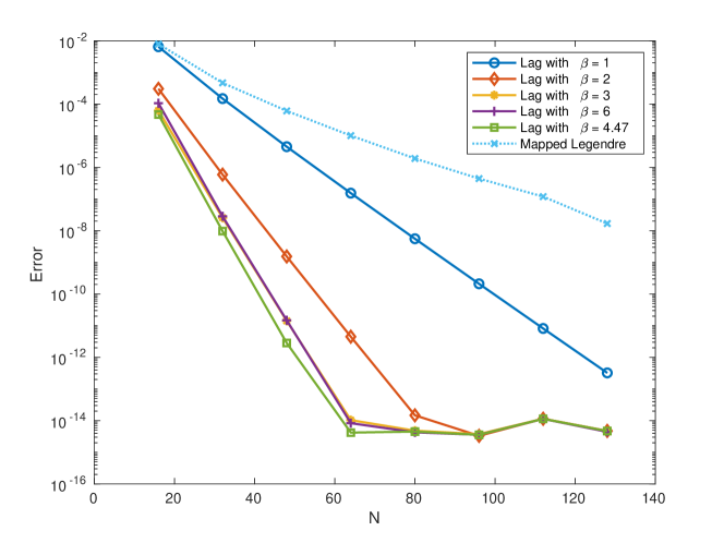
Figure 6: Numerical errors of the Laguerre method solving equation (37) with $\gamma=2$ and exact solution $u_{1}(x)=\sin(2x)e^{-x}$ using different values for scaling constant $\beta$, and compared with the mapped Legendre method.

For functions having other decaying properties, it is not easy to obtain an explicit formula for the optimal value of the scaling factor $\beta$. We leave the problem of finding optimal scaling of the Laguerre method for general functions to a future study.

4.3 Using more than one thousand Laguerre bases

In previous numerical studies using Laguerre methods for unbounded domains, only small numbers of Laguerre bases are used due to the fact that the standard methods to generate Laguerre polynomials and Laguerre functions encounter serious round-off error and overflow/underflow issues, which are explained in last section. Now, we apply the improved Laguerre algorithms to solve equation (37) with algebraic decay solutions $u_{2}$ and $u_{3}$. It is known that the convergence rate is also algebraic [23, 26], thus, one may need a lot of Laguerre bases to get good numerical results when the rate is slow.

In Figure 7, we present the results of using scaled Laguerre method and mapped Legendre method for (37) with exact solution $(1+x)^{-5/2}$. Note that, the tested case is same to the right plot of Figure 8 in [26], where only 128 bases are used. Here, 1024 Laguerre bases are used, which show more clear the convergence behavior of the Laguerre method. In particular, Laguerre method with $\beta=0.6$ and 1024 bases leads to $L^{2}$ error smaller than $3\times 10^{-13}$. From Figure 7, we see if a smaller value of $\beta$ is used, one needs use more degree of freedoms to pass through a larger pre-asymptotic range to get the algebraic convergence rate. We also observe that larger scaling factor $\beta$ should be used with less Laguerre bases, and smaller $\beta$ should be used with large numbers of Laguerre bases. This is different to the exponential decay case. It can be observed that the converge of Laguerre method for this test case is slower than the mapped Legendre method, this is consistent to the theoretical result [26].

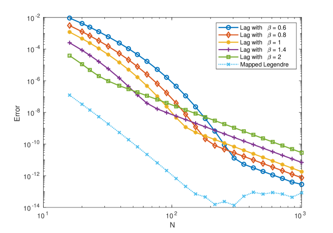
Figure 7: Convergence results of the scaled Laguerre method and mapped Legendre method solving equation (37) with $\gamma=2$ and exact solution $u_{2}(x)=(1+x)^{-5/2}$. The $L^{2}$ error is shown.

In Figure 8, we show numerical results for algebraic decay solutions with oscillations. Here, we take $u_{3}(x)=\sin(2x)(1+x)^{-7/2}$. It is observed that the convergence speed of the Laguerre method with best scaling factor is better than the mapped Legendre method. We also observe that the best scaling factor is not sensitive to the number of bases used, which means that we can tune the scaling factor on coarse grids and use the result on refined grids.

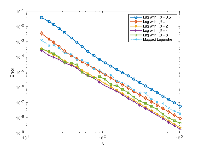
Figure 8: Convergence results of the scaled Laguerre method and mapped Legendre method solving equation (37) with $\gamma=2$ and exact solution $u_{3}(x)=\sin(2x)(1+x)^{-7/2}$. The $L^{2}$ error is shown.

5 Conclusion

In this paper, we proposed improved algorithms to generate Laguerre polynomials, Laguerre functions as well as Laguerre-Gauss quadrature schemes with better stability and smaller round-off errors, which are essential to Laguerre methods for solving partial differential equations in unbounded domains. These algorithms can stably generate Laguerre functions of degree higher than one thousand using floating-point number systems with much smaller numerical errors than existing methods. With the help of these basic algorithms, one may use thousands of bases in the Laguerre spectral methods to get better numerical results. We have demonstrated this by considering the Laguerre spectral method solving an elliptic equation defined on $\mathbb{R}_{+}$. We also presented some analysis and numerical investigations on the optimal scaling factor of the Laguerre spectral methods. We found that in the two special cases that the Laguerre method converges faster than the mapped Legendre method, the optimal scaling factor is independent of the numerical resolutions, which suggests that one can tune the scaling factor using coarse grids and use the results on refined grids.

References

• [1] M. Abramowitz and I. A. Stegun, Handbook of Mathematical Functions with Formulas, Graphs, and Mathematical Tables, U.S. Department of Commerce, 1972.
• [2] M. Azaiez, J. Shen, C. Xu, and Q. Zhuang, A Laguerre-Legendre spectral method for the Stokes problem in a semi-infinite channel, SIAM J. Numer. Anal., 47 (2009), pp. 271–292, https://doi.org/10.1137/070698269.
• [3] W. Bao and J. Shen, A fourth-order time-splitting Laguerre–Hermite pseudospectral method for Bose–Einstein condensates, SIAM J. Sci. Comput., 26 (2005), pp. 2010–2028, https://doi.org/10.1137/030601211.
• [4] W. Bao and J. Shen, A generalized-Laguerre–Hermite pseudospectral method for computing symmetric and central vortex states in Bose–Einstein condensates, Journal of Computational Physics, 227 (2008), pp. 9778–9793, https://doi.org/10.1016/j.jcp.2008.07.017.
• [5] A. H. Bhrawy, D. Baleanu, and L. M. Assas, Efficient generalized Laguerre-spectral methods for solving multi-term fractional differential equations on the half line, Journal of Vibration and Control, 20 (2014), pp. 973–985, https://doi.org/10.1177/1077546313482959.
• [6] J. P. Boyd, Asymptotic coefficients of Hermite function series, Journal of Computational Physics, 54 (1984), pp. 382–410, https://doi.org/10.1016/0021-9991(84)90124-4.
• [7] C. Canuto, M. Y. Hussaini, A. Quarteroni, and T. A. Zang, Spectral Methods: Evolution to Complex Geometries and Applications to Fluid Dynamics, Scientific Computation, Springer-Verlag, Berlin, 2007.
• [8] F. Chen, J. Shen, and H. Yu, A new spectral element method for pricing european options under the Black-Scholes and Merton jump diffusion models, Journal of Scientific Computing, (2012), pp. 1–20, https://doi.org/10.1007/s10915-011-9556-5.
• [9] S. Chen, J. Shen, and L.-L. Wang, Laguerre functions and their applications to tempered fractional differential equations on infinite intervals, Journal of Scientific Computing, 74 (2018), pp. 1286–1313, https://doi.org/10.1007/s10915-017-0495-7.
• [10] D. Funaro, Computational aspects of pseudospectral Laguerre approximations, Applied Numerical Mathematics, 6 (1990), pp. 447–457, https://doi.org/10.1016/0168-9274(90)90003-x.
• [11] W. Gautschi, Orthogonal polynomials: Applications and computation, Acta Numerica, 5 (1996), pp. 45–119, https://doi.org/10.1017/S0962492900002622.
• [12] G. H. Golub and J. H. Welsch, Calculation of Gauss quadrature rules, Math. Comp., 23 (1969), pp. 221–230, https://doi.org/10.1090/S0025-5718-69-99647-1.
• [13] D. Gottlieb and S. A. Orszag, Numerical Analysis of Spectral Methods: Theory and Applications, SIAM, 1977.
• [14] B. Guo and Z. Wang, Numerical integration based on Laguerre-Gauss interpolation, Computer Methods in Applied Mechanics and Engineering, 196 (2007), pp. 3726–3741, https://doi.org/10.1016/j.cma.2006.10.035.
• [15] B. Y. Guo and H. P. Ma, Composite Legendre-Laguerre approximation in unbounded domains, J. Comput. Math., 19 (2001), pp. 101–112.
• [16] B.-Y. Guo and J. Shen, Laguerre-Galerkin method for nonlinear partial differential equations on a semi-infinite interval, Numerische Mathematik, 86 (2000), pp. 635–654, https://doi.org/10.1007/pl00005413.
• [17] B.-Y. Guo, Z.-Q. Wang, H.-J. Tian, and L.-L. Wang, Integration processes of ordinary differential equations based on Laguerre-Radau interpolations, Math. Comp., 77 (2008), pp. 181–199, https://doi.org/10.1090/S0025-5718-07-02035-2.
• [18] F.-j. Liu, H.-y. Li, and Z.-q. Wang, Spectral methods using generalized Laguerre functions for second and fourth order problems, Numer Algor, 75 (2017), pp. 1005–1040, https://doi.org/10.1007/s11075-016-0228-2.
• [19] F.-J. Liu, Z.-Q. Wang, and H.-Y. Li, A fully diagonalized spectral method using generalized Laguerre functions on the half line, Adv Comput Math, 43 (2017), pp. 1227–1259, https://doi.org/10.1007/s10444-017-9522-3.
• [20] H. Ma, W. Sun, and T. Tang, Hermite spectral methods with a time-dependent scaling for parabolic equations in unbounded domains, SIAM J. Numer. Anal., 43 (2005), pp. 58–75, https://doi.org/10.1137/s0036142903421278.
• [21] M. Masoumnezhad, M. Saeedi, H. Yu, and H. S. Nik, A Laguerre spectral method for quadratic optimal control of nonlinear systems in a semi-infinite interval, Automatika, 61 (2020), pp. 461–474, https://doi.org/10.1080/00051144.2020.1774724.
• [22] F. W. J. Olver, ed., NIST Handbook of Mathematical Functions, Cambridge University Press : NIST, Cambridge ; New York, 2010.
• [23] J. Shen, Stable and efficient spectral methods in unbounded domains using Laguerre functions, SIAM J. Numer. Anal., 38 (2000), pp. 1113–1133, https://doi.org/10.1137/S0036142999362936.
• [24] J. Shen, T. Tang, and L.-L. Wang, Spectral Methods: Algorithms, Analysis and Applications, no. 41 in Springer Series in Computational Mathematics, Springer, Heidelberg ; New York, 2011.
• [25] J. Shen and L.-L. Wang, Laguerre and composite Legendre-Laguerre dual-Petrov-Galerkin methods for third-order equations, Discrete & Continuous Dynamical Systems - B, 6 (2006), p. 1381, https://doi.org/10.3934/dcdsb.2006.6.1381.
• [26] J. Shen and L.-L. Wang, Some recent advances on spectral methods for unbounded domains, Commun. Comput. Phys, 5 (2009), pp. 195–241.
• [27] J. Shen, Y. Wang, and H. Yu, Efficient spectral-element methods for the electronic Schr\”odinger equation, in Sparse Grids and Applications-Stuttgart 2014, Springer, 2016, pp. 265–289.
• [28] G. Szegő, Orthogonal Polynomials, vol. 23 of Colloquium Publications, American Mathematical Society, Providence, Rhode Island, 4th edition ed., 1975, https://doi.org/10.1090/coll/023.
• [29] T. Tang, The Hermite spectral method for Gaussian-type functions, SIAM Journal on Scientific Computing, 14 (1993), pp. 594–594, https://doi.org/10.1137/0914038.
• [30] T. Tang, H. Yuan, and T. Zhou, Hermite spectral collocation methods for fractional PDEs in unbounded domains, Commun. Comput. Phys., 24 (2018), pp. 1143–1168, https://doi.org/10.48550/arXiv.1801.09073, https://arxiv.org/abs/1801.09073.
• [31] T.-j. Wang and B.-y. Guo, Composite generalized Laguerre-Legendre pseudospectral method for Fokker-Planck equation in an infinite channel, Applied Numerical Mathematics, 58 (2008), pp. 1448–1466, https://doi.org/10.1016/j.apnum.2007.08.007.
• [32] M. Xia, S. Shao, and T. Chou, Efficient scaling and moving techniques for spectral methods in unbounded domains, SIAM J. Sci. Comput., 43 (2021), pp. A3244–A3268, https://doi.org/10.1137/20M1347711.
• [33] C.-l. Xu and B.-y. Guo, Mixed Laguerre-Legendre spectral method for incompressible flow in an infinite strip, Advances in Computational Mathematics, 16 (2002), pp. 77–96, https://doi.org/10.1023/A:1014249613222.
• [34] C. Zhang, D.-q. Gu, Z.-q. Wang, and H.-y. Li, Efficient space-time spectral methods for second-order problems on unbounded domains, J Sci Comput, 72 (2017), pp. 679–699, https://doi.org/10.1007/s10915-017-0374-2.