Competing types in preferential attachment graphs with community structure

Abstract

We extend the two-type preferential attachment model of Antunović, Mossel and Rácz to networks with community structure. We show that different types of limiting behaviour can be found depending on the choice of community structure and type assignment rule.

In particular, we show that, for essentially all type assignment rules where more than one limit has positive probability in the unstructured model, communities may simultaneously converge to different limits if the community connections are sufficiently weak. If only one limit is possible in the unstructured model, this behaviour still occurs for some choices of type assignment rule and community structure. However, we give natural conditions on the assignment rule and, for two communities, on the structure, either of which will imply convergence to this limit, and each of which is essentially best possible.

Although in the unstructured two-type model convergence almost surely occurs, we give an example with community structure which almost surely does not converge.

1 Introduction

In [3], Antunović, Mossel and Rácz introduced a model for preferential attachment graphs where each vertex is of one of a number of types, which may, for example, be thought of as brand preferences. Each vertex chooses its type based on the types of its neighbours when it joins the network. In this paper, we will concentrate on the setting with two types, which we refer to as “red” and “blue”, and standard preferential attachment. Antunović, Mossel and Rácz [3] showed that in this setting the proportion of red vertices converges to a limit. In the “linear model” this limit is distributed with full support on $[0,1]$, whereas in non-linear models there are finitely many possible limits corresponding to stable zeros of a particular polynomial $P$, defined later, which depends on the type assignment rule.

The purpose of this paper is to extend the analysis of [3] to preferential attachment models with community structure. The model we use is the model for geometric preferential attachment graphs in Jordan [14], in the special case where the space $S$ the graphs are embedded in is a finite set; each element of $S$ can then be thought of as a community, as described by Hajek and Sankagiri in [12].

A natural question in this setting is whether different communities can show different limiting behaviour for the proportions of types within them. We will answer this question in the affirmative, showing (Theorem 1) that where the polynomial $P$ defined by the type assignment rule has multiple stable zeros there is, assuming some natural conditions on the type assignment rule, positive probability of different limits in different communities if the interaction between the communities is sufficiently weak.

We will also show (Theorems 3 and 4) that, again under some natural conditions on the interaction between the communities and the type assignment rule, this does not occur if the polynomial $P$ has only one stable zero (corresponding to only one limit having positive probability in the model of [3]) and that in this the proportions of red in each community will all converge to the same limit. However, we will also show some examples, with perhaps less natural choices of community interaction and type assignment rule, where multiple limits are possible even in this case.

Based on the results in [3] for a single community, it might be expected that for any stable zero of the polynomial $P$ there would be positive probability that there would be convergence of the proportions of red vertices in each community to that zero. It turns out that in the multi community set-up this is not necessarily the case, and indeed we will show an example (Proposition 6) where the proportions of types in the different communities almost surely do not converge to limits. However, we will give a result (Theorem 5) with an extra condition on $P$ in the neighbourhood of the zero which ensures that there is positive probability of all communities converging to it.

Finally, we will show (Theorem 8) that, as long as there are enough non-zero interactions between communities, in the linear model (where $P$ is the zero polynomial) convergence to different limits does not occur and all communities synchronise to the same random limit; compare the synchronisation of Pólya urns with a network structure found in Dai Pra, Louis and Minelli [8].

We mention some related work and some possible extensions. The broadcasting problem studied by Addagio-Berry, Devroye, Lugosi and Velona [1] on the preferential attachment tree is a special case of the model of [3], while Backhausz and Rodner [4] consider a model where it is the edges rather than the vertices which have types. The model of [14] is more generally a geometric preferential attachment model with vertices embedded in a metric space $S$ as in Flaxman, Frieze and Vera [10, 11] and Manna and Sen [16]. Given our results for the case where $S$ is finite, a natural question is whether different limits may be possible in different parts of $S$ when $S$ is an uncountable metric space such as a torus. A degenerate case of geometric preferential attachment is the online nearest neighbour graph, as discussed in [15] and [16] (where it is considered as the “$\alpha=-\infty$” case). A simple type assignment process on the online nearest neighbour graph, where each vertex takes the type of its nearest neighbour when it joins the graph, is equivalent to the partitions model studied by Aldous in [2], where it is shown that the process converges in a suitable sense to a random partition of the underlying set; this might suggest that similar phenomena might occur for at least some geometric preferential attachment models.

The structure of the paper is as follows. We define our framework in section 2 and state our results in section 3, with proofs of the results in section 4. Finally in section 5 we consider some examples which illustrate our results, show some simulations, and give some more detailed calculations which are specific to those examples.

2 Definitions and notation

2.1 Graph model

Our graph model is the model of [14] with the space $S$ considered to be a finite set, the elements each corresponding to a community, with $N=|S|$ being the number of communities. Each vertex is assigned to an element of $S$ according to a probability measure $\mu$ independently of other vertices and of the growth of the graph before it is added. A parameter $m$ governs the number of new connections formed by each vertex as it joins the graph.

In addition, there is an attractiveness function, defined by an $N\times N$ matrix $A$ with entries $(\alpha_{x,y})_{x,y\in S}$ such that the relative attractiveness of an existing vertex in community $x$ to a new vertex in community $y$ is $\alpha_{x,y}\geq 0$. (In many cases, $A$ will be a symmetric matrix, but this is not necessary in [14].) We allow an individual attractiveness coefficient $\alpha_{x,y}$ to be $0$, in which case a new vertex in community $y$ will never attach to a vertex in community $x$ (though if $\alpha_{x,y}>0$ edges may form between the two communities in the opposite way). However, for each community $y$ we require $\sum_{x}\alpha_{x,y}>0$, since a new vertex in community $y$ must attach somewhere.

The preferential attachment graph evolves from an initial graph $G_{0}$, with $n_{0}$ vertices, such that $G_{0}$ contains at least one vertex in each community and all vertices have positive degree. The graph $G_{t+1}$ is produced from $G_{t}$ by creating a new vertex $v_{t+1}$ and assigning it to a community $c(v_{t+1})$. We then choose $m$ existing vertices independently at random (with replacement), with the probability of choosing a vertex $v_{s}$ being

$$\frac{\alpha_{c(v_{s}),c(v_{t+1})}\deg_{G_{t}}(v_{s})}{\sum_{u\in V(G_{t})}\alpha_{c(u),c(v_{t+1})}\deg_{G_{t}}(u)},$$ (1)

and form edges from $v_{t+1}$ to the $m$ vertices chosen (note that this may involve multiple edges between the same pair of vertices). For notational convenience we assume the initial graph $G_{0}$ has $mn_{0}$ edges.

2.2 Type assignment

After joining the graph and forming edges, each vertex chooses one of two types, which we refer to as “red” and “blue”. The choice of type is based on the types of its neighbours according to some rule, which may be random. This formulation allows the same type assignment rules as in [3] to be considered, and we will use the same notation for the type assignment mechanism; in particular in the case with two types the probability that a new vertex becomes red, conditional on having $k$ red neighbours, is $p_{k}$. (Because the new vertex makes $m$ connections in total, the probability that a new vertex with $k$ blue neighbours becomes blue is $1-p_{m-k}$. Type assignment mechanisms with $p_{k}=1-p_{m-k}$ thus have symmetry between the two types.)

The special case where $p_{k}=\frac{k}{m}$ for all $k$ is referred to as the linear model in [3]. The model studied in [3] is as described above but with the graph growing according to a standard preferential attachment model, specifically the independent model described in [6], which is the special case of the model of [14] with only one community; we will refer to it in this paper as the single community model.

Remark.

It is of course possible to consider a version of this model with more than two types, and this was considered in section 3 of [3], although that paper focussed mainly on the two type case. With more than two types there is potential for more complicated behaviour, and Haslegrave and Jordan [13] gave an example with non-convergence in that case. We might therefore expect that there are interesting examples with multiple communities and more than two types, but we leave this for future work and focus on two types in this paper.

We will associate the rule given by $p_{0},\cdots,p_{m}$ with the polynomial given by

$$R(z)=\sum_{i=0}^{m}\binom{m}{i}z^{i}(1-z)^{m-i}p_{i},$$

that is, $R(z)$ is the probability of a vertex becoming red if its neighbours are independently red with probability $z$.

This polynomial allows us to describe the behaviour of the single-community model. Except for the linear model where $R(z)\equiv z$, the possible limits for the proportion of red vertices are the fixed points of $R$; in the linear model the limit is a random variable with full support on $(0,1)$. This was proved in [3], although they instead considered the zeroes of $P(z)=(R(z)-z)/2$.

To understand the possible limits for the single community model further, for a fixed point $z\in(0,1)$ of $R$ we classify it as stable if there exists $\varepsilon>0$ such that $R(y)>y$ for $y\in(z-\varepsilon,z)$ and $R(y)<y$ for $y\in(z,z+\varepsilon)$, as unstable if there exists $\varepsilon>0$ such that $R(y)<y$ for $y\in(z-\varepsilon,z)$ and $R(y)>y$ for $y\in(z,z+\varepsilon)$, and as a touchpoint if there exists $\varepsilon>0$ such that $R(y)-y$ is either strictly positive or strictly negative on $(z-\varepsilon,z)\cup(z,z+\varepsilon)$. Similarly $z=0$ is a stable fixed point of $R$ if $R(0)=0$ and there exists $\varepsilon>0$ such that $R(y)<y$ for $y\in(0,\varepsilon)$, and is an unstable fixed point of $R$ if $R(0)=0$ and there exists $\varepsilon>0$ such that $R(y)>y$ if $y\in(0,\varepsilon)$; similar definitions apply to a fixed point at $z=1$. We say that a stable fixed point $z$ is linearly stable if the derivative $R^{\prime}(z)<1$, and that an unstable fixed point $z$ is linearly unstable if $R^{\prime}(z)>1$. It is shown in [3] that in the single community model the proportion of red edge-ends converges almost surely and that the limit is either a stable fixed point or a touchpoint of $R$, with all such points having positive probability of being the limit.

3 Results

Our results are concerned with the limiting proportion of red edge-ends in each community (if the limit exists). Equivalently this is the probability that a vertex selected according to (1) is red, conditional on it being in that community, and as a result almost sure convergence of the proportions of edge ends in each community which are red implies the same for proportions of vertices in each community.

Write $Z^{(n)}_{i}$ for the proportion of edge-ends in community $i$ at time $n$ which are at red vertices, that is

$$Z^{(n)}_{i}=\frac{\sum_{v\text{ red, }c(v)=i}\deg_{G_{n}}(v)}{\sum_{v:c(v)=i}\deg_{G_{n}}(v)}.$$

Our first result shows that under certain conditions we do get positive probability of different limits in different communities. It will be useful to consider the following family of attractiveness matrices: given a matrix $A_{1}$, with all diagonal elements positive, let $A_{0}$ be a diagonal matrix whose diagonal elements are the same as those of $A_{1}$, and then for $\theta>0$ define $A_{\theta}=(1-\theta)A_{0}+\theta A_{1}$; changing the value of $\theta$ allows tuning of the relative strength of the inter-community and intra-community interactions. Then the following theorem shows that for sufficiently small but positive $\theta$, there is positive probability that the proportion of red edge ends in community $1$ converges to a limit close to $z_{1}$ while the proportion of red edge ends in community $2$ converges to a limit close to $z_{2}$.

Theorem 1.

Assume that the polynomial $R$ has two distinct linearly stable fixed points, $z_{1}$ and $z_{2}$. Then for any choice of interaction matrix $A_{1}$, and any $\varepsilon>0$, there exists $\theta_{\varepsilon}>0$ such that for $\theta<\theta_{\varepsilon}$ the system with interaction matrix $A_{\theta}$ has positive probability that $Z^{(1)}_{n}\to\tilde{z}_{1}$ and $Z^{(2)}_{n}\to\tilde{z}_{2}$ as $n\to\infty$, where $\lvert z_{1}-\tilde{z}_{1}\rvert,\lvert z_{2}-\tilde{z}_{2}\rvert<\varepsilon$.

In particular, there is some $\theta_{\mathrm{crit}}>0$ such that for $\theta<\theta_{\mathrm{crit}}$ there is positive probability of convergence to different limits.

Theorem 1 cannot in general be extended to the case where $R$ has one stable fixed point and one touchpoint, even though in this case the single-community model has more than one possible limit.

Proposition 2.

Suppose that the polynomial $R$ has a unique stable fixed point $z^{*}$, and some touchpoints. Let $A_{1}$ be any interaction matrix with all entries positive. Then for $\theta$ sufficiently small, in the the system with interaction matrix $A_{\theta}$ convergence to different limits has probability zero.

Examples of this type where different limits having both probability zero and positive probability will be considered in section 5.

Our second main result gives some situations where the communities will all have the same limit.

Theorem 3.

Assume that $z^{*}$ is the only fixed point of $R$ in $[0,1]$, except possibly for linearly unstable fixed points at $0$ and/or $1$.

1. Suppose that the type assignment rule is such that the only fixed points of $R(R(z))$ in $[0,1]$ are the fixed points of $R(z)$. Then for all communities $i$ we have $Z^{(n)}_{i}\to z^{*}$ as $n\to\infty$, almost surely.

2. Conversely, suppose that the type assignment rule is such that $R(R(z))$ has a linearly stable fixed point $\tilde{z}\neq z^{*}$. Then for the community structure (with two communities) given by

   $$A=\begin{pmatrix}0&1\\ 1&0\end{pmatrix}$$

   and any $\mu_{1},\mu_{2}>0$ with $\mu_{1}+\mu_{2}=1$, there is positive probability that there exist $z_{1}\neq z_{2}$ such that $Z^{(n)}_{1}\to z_{1}$ and $Z^{(n)}_{2}\to z_{2}$.

Remark.

We note that the condition on the rule in the first part of Theorem 3 is satisfied by any increasing rule for which $R$ has a unique fixed point; here we say that a rule is increasing if $R(z)$ is increasing in $z$. Since $R(z)$ may be expressed as $\mathbb{E}(p_{K})$ where $K\sim\operatorname{Bin}(m,z)$, any rule for which $p_{k}$ is increasing in $k$ is necessarily an increasing rule; however, the rule being increasing is a strictly weaker condition. For example, when $m=3$ the rule given by $p_{0}=0,p_{1}=1,p_{2}=0,p_{3}=1$ is increasing, since $R(z)=z^{3}+3z(1-z)^{2}$, and so $R^{\prime}(z)=3(1-2z)^{2}\geq 0$. All rules considered in [3] in fact have $p_{k}$ increasing in $k$ and thus are increasing rules.

In the case where there are two communities, we can also give a necessary and sufficient condition on the matrix such that convergence to $z^{*}$ happens in both communities for any type assignment rule with a single zero, which is stable.

Theorem 4.

Consider the two-community case, i.e. $S=\{1,2\}$.

1. Suppose $\det A\geq 0$, and the type assignment rule is such that $z^{*}$ is the only fixed point of $R$ in $[0,1]$, except possibly for linearly unstable fixed points at $0$ and/or $1$. Then for each $i\in\{1,2\}$ we have $Z^{(n)}_{i}\to z^{*}$ as $n\to\infty$, almost surely.

2. Conversely, suppose $\det A<0$. Then there exists a type assignment rule such that $R$ has a unique fixed point $z^{*}\in[0,1]$ but for which there is positive probability that there exist $z_{1}\neq z_{2}$ such that $Z^{(n)}_{1}\to z_{1}$ and $Z^{(n)}_{2}\to z_{2}$.

The methods used to prove Theorem 3 also give the following result, which shows that for stable fixed points of $R$ where $R$ is locally increasing there is positive probability that all communities converge to them; in particular this will apply to any stable fixed point of $R$ when the rule is increasing.

Theorem 5.

Let $z^{*}$ be a stable fixed point of the polynomial $R$ such that $R$ is increasing in some neighbourhood of $z^{*}$. Then there is positive probability that $Z^{(n)}_{i}\to z^{*}$ for all $i$.

Some condition beyond stability is necessary in Theorem 5. Indeed, it is possible to find examples which do not even converge to a limit; the following result gives such an example.

Proposition 6.

Let $S=\{1,2,3\}$ and

$$A=\begin{pmatrix}0&1&0\\ 0&0&1\\ 1&0&0\end{pmatrix}$$

(representing three communities in a cycle, with each only influenced by the one clockwise of it), with $\mu_{i}=\frac{1}{3}$ for $i=1,2,3$. Let $m$ be an odd integer, and let the $p_{k}$ be given by the minority rule: $p_{k}=1$ for $0\leq k\leq\frac{m-1}{2}$ and $p_{k}=0$ for $\frac{m+1}{2}\leq k\leq m$. Then for $m\geq 7$ almost surely $\bigl{(}Z^{(1)}_{n},Z^{(2)}_{n},Z^{(3)}_{n}\bigr{)}$ does not converge to a limit.

Figure 1 shows a simulation of proportions of red in each community over time in the framework of Proposition 6 for $m=7$. It appears that the process is converging instead to a limit cycle.

This example raises the following natural question.

Question 7.

Is there an example with only two communities which fails to converge with positive probability?

Finally, we consider the linear model. Here we have the following result, which shows that in this setting we do not get different limits in different communities for typical community structures. To state it we need to consider the directed graph $\Gamma$ whose vertex set is $S$ and which has an edge from $i$ to $j$ if and only if $\alpha_{j,i}>0$.

Theorem 8.

Assume that $\Gamma$ is such that for any two vertices $i$ and $j$ there is a vertex $h$ such that there are directed paths from both $i$ and $j$ to $h$. (We allow $h=i$ or $h=j$, and treat any vertex $i$ as having a directed path to itself.) Then in the linear model with $p_{k}=\frac{k}{m}$ for all $k$, there exists a random limit $M$ such that $Z^{(n)}_{i}\to M$ for all $i$.

Remark.

The condition on $\Gamma$ is equivalent to stating that a random walk on $\Gamma$, treating it as a directed graph, has a unique stationary distribution. It is also equivalent to the directed graph with every edge reversed being quasi strongly connected as defined, for example, in Chapter 5 of [18].

Figure 1: The values of $Z^{(t)}_{1},Z^{(t)}_{2},Z^{(t)}_{3}$ in the framework of Proposition 6 with $m=7$ plotted over time (log scale), showing apparent non-convergence.

4 Proofs

4.1 Stochastic approximation

The methods used in [3] rely heavily on the theory of stochastic approximation, relating the dynamics of the proportion of edge ends which are red to those of the differential equation driven by the polynomial $P(z)=(R(z)-z)/2$. In this section we show how to set the process up as a multi-dimensional stochastic approximation process and identify the driving vector field; this will be useful for some of our proofs and specific examples. Note that zeroes of $P$ correspond to fixed points of $R$, and vice versa; we will describe a zero of $P$ as (linearly) stable, (linearly) unstable or a touchpoint according to the behaviour of the corresponding fixed point of $R$.

Let $X^{(n)}_{i,j}$, $i=1,\ldots,N$, $j=1,2$, be the proportion of edge-ends of $G_{n}$ which are in community $i$ and at a vertex of type $j$; $j=1$ will correspond to red and $j=2$ to blue. Let $\mathbf{X}^{(n)}=\bigl{(}X^{(n)}_{1,1},X^{(n)}_{1,2},\ldots,X^{(n)}_{N,1},X^{(n)}_{N,2}\bigr{)}$, and note that this takes values in the set

$$\Delta^{2N-1}=\biggl{\{}(x_{1,1},x_{1,2},\ldots,x_{N,1},x_{N,2})\in\bigl{(}\mathbb{R}_{\geq 0}\bigr{)}^{2N}:\sum\nolimits_{i=1}^{N}(x_{i,1}+x_{i,2})=1\biggr{\}},$$

which is a $(2N-1)$-dimensional set. Write $Y^{(n)}_{i}=X^{(n)}_{i,1}+X^{(n)}_{i,2}$ for the total proportion of edge-ends in community $i$; note that this means $Y^{(n)}_{i}Z^{(n)}_{i}=X^{(n)}_{i,1}$.

The probability, conditional on $G_{n}$ and that the new vertex at time $n+1$ is in community $i$, that a specific edge from that vertex connects to a vertex of type $j$ is $Q_{i,j}(\mathbf{X}^{(n)})$, where for $x\in\Delta^{2N-1}$ we define

$$Q_{i,j}(x)=\frac{\sum_{k=1}^{N}\alpha_{k,i}x_{k,j}}{\sum_{k=1}^{N}\alpha_{k,i}x_{k,1}+\sum_{k=1}^{N}\alpha_{k,i}x_{k,2}}.$$

Thus the probability that a new vertex at location $i$ at time $n+1$ becomes red (type $1$) is $R(Q_{i,j}(x))$, and so the contribution to the expected number of new edge ends of type $1$ at location $i$ at time $n+1$ coming from the new vertex, conditional on $G_{n}$, can be written $G_{i,1}(\mathbf{X}^{(n)})$, where for $x\in\Delta^{2N-1}$ we define $G_{i,1}(x)=m\mu_{i}R\left(Q_{i,1}(x)\right)$.

Similarly we define $G_{i,2}(x)=m\mu_{i}(1-R(1-Q_{i,2}(x))$, so that $G_{i,2}(\mathbf{X}^{(n)})$ is the contribution to the expected number of new edge ends of type $2$ at location $i$ at time $n+1$ coming from the new vertex, conditional on $G_{n}$; this uses the fact that the probability a new vertex is blue (type 2) given that it has $k$ blue neighbours is $1-p_{m-k}$.

The contribution to the expectation coming from the edge ends at the existing vertices is $H_{i,j}(\mathbf{X}^{(n)})$ where for $x\in\Delta^{2N-1}$ we define

$$H_{i,j}(x)=mx_{i,j}\sum_{k=1}^{N}\mu_{k}\frac{\alpha_{i,k}}{\sum_{\ell=1}^{N}\alpha_{\ell,k}\left(x_{\ell,1}+x_{\ell,2}\right)}.$$

Hence we can write

$$X^{(n+1)}_{i,j}-X^{(n)}_{i,j}=\gamma_{n}(F_{i,j}(\mathbf{X}_{n})+\xi^{(n+1)}_{i,j})$$

where, again for $x\in\Delta^{2N-1}$,

$$F_{i,j}(x)=G_{i,j}(x)+H_{i,j}(x)-2mx_{i,j},$$

and where $\gamma_{n}^{-1}=2m(n+n_{0}+1)$ and the $\xi^{(n+1)}_{i,j}$ are noise terms with $\mathbb{E}(\xi^{(n+1)}_{i,j}\mid\mathcal{F}_{n})=0$, and so $(\mathbf{X}_{n})_{n\geq 0}$ is a Robbins-Monro stochastic approximation process as defined in section 4.2 of Benaïm [5]. Furthermore, because exactly $2m$ edge ends are added at each time point, each component of the noise term $\xi^{(n+1)}_{i,j}$ is uniformly bounded in modulus by $2m$, which means that we can apply Proposition 4.2 of [5] to show that $(\mathbf{X}_{n})_{n\geq 0}$ is an asymptotic pseudotrajectory of the vector field on $\Delta^{2N-1}$ driven by $F$.

From results in [14], for each $i\in\{1,\ldots,N\}$ the limit as $n\to\infty$ of the proportion of edge ends in community $i$, $X^{(n)}_{1,1}+X^{(n)}_{1,2}$, almost surely converges to a particular limit $\nu_{i}$, where the $\nu_{i}$ are the unique solution satisfying $\nu_{i}\in[0,1]$ for all $i$ and $\sum_{i=1}^{N}\nu_{i}=1$ to the equations

$$\nu_{i}=\frac{1}{2}\mu_{i}+\frac{1}{2}\sum_{j=1}^{N}\mu_{j}\frac{a_{i,j}\nu_{j}}{\sum_{k=1}^{N}a_{k,j}\nu_{k}}.$$ (2)

The consequence of this result for our situation is that the limit set of $(\mathbf{X}_{n})$ must be contained within the set

$$\Delta_{\nu}=\{(x_{1,1},x_{1,2},\ldots,x_{N,1},x_{N,2})\in\Delta^{2N-1}:x_{1,1}+x_{1,2}=\nu_{1},\ldots,x_{N,1}+x_{N,2}=\nu_{N}\}.$$

This will be useful in some examples when it comes to identifying possible limits.

In many cases the equations (2) for the $\nu_{i}$ do not have a closed form solution, but there are some examples where they do; for example when $\mu_{i}=\frac{1}{N}$ for all $i$ and the matrix $A$ has suitable symmetries it can be seen that $\nu_{i}=\frac{1}{N}$ for all $i$.

4.2 Proof of Theorem 1

Let $z_{1}$ be the smallest linearly stable fixed point of the polynomial $R$, and $z_{2}>z_{1}$ be the largest. Linear stability ensures that $R^{\prime}(z_{1}),R^{\prime}(z_{2})<1$. We may assume $\varepsilon$ is sufficiently small that $R(z)$ has no other fixed points within $\varepsilon$ of $z_{1}$ or $z_{2}$, and that $R^{\prime}(z)<1-\kappa$ in this range for some $\kappa>0$.

Without loss of generality, we may assume that the diagonal elements of $A_{\theta}$ are all $1$, and we write the off-diagonal entries of $A_{1}$ as $\tilde{\alpha}_{i,j}$ so that the off-diagonal entries of $A_{\theta}$ are $\alpha_{i,j}=\theta\tilde{\alpha}_{i,j}$.

We partition $S$ into two non-empty sets $S_{1}$ and $S_{2}$, and we will prove that with positive probability all communities whose labels are in $S_{i}$ have proportions of red converging to limits within $\varepsilon$ of $z_{i}$.

Let $R^{(i)}_{t}$ (respectively, $B^{(i)}_{t}$) be the number of red (respectively, blue) edge-ends in community $i$ at time $t$. For each $i\in S_{1}$, we will define an urn process with $R^{\prime(i)}_{t}$ red balls and $B^{\prime(i)}_{t}$ blue balls, which will give an upper bound on the proportion of red in community $i$. We initialise the urns at some time $t_{0}$ to be chosen later, such that $R^{\prime(i)}_{t_{0}}=R^{(i)}_{t_{0}}$ and $B^{\prime(i)}_{t_{0}}=B^{(i)}_{t_{0}}$.

Fix $\delta_{0}>0$ to be smaller than $\min_{i}\nu_{i}$. We will show by induction that, provided

$$\lvert Y^{(i)}_{t}-\nu_{i}\rvert<\delta_{0},\text{ for all }i\text{ and for all }t\geq t_{0},$$ (3)

we may couple the two processes such that $R^{\prime(i)}_{t}+B^{\prime(i)}_{t}\geq R^{(i)}_{t}+B^{(i)}_{t}$ and $B^{\prime(i)}_{t}\leq B^{(i)}_{t}$ for each $t\geq t_{0}$. Write $r^{\prime}=\frac{R^{\prime(i)}_{t}}{R^{\prime(i)}_{t}+B^{\prime(i)}_{t}}$ and $r=\frac{R^{(i)}_{t}}{R^{(i)}_{t}+B^{(i)}_{t}}$; it follows that $r^{\prime}\geq r$. In the analysis that follows, we assume (3) holds.

For $i\in S$, set

$$q_{i,i}^{-}=\frac{\nu_{i}-\delta_{0}}{(\nu_{i}-\delta_{0})+\sum_{k\in S\setminus\{i\}}\theta\tilde{\alpha}_{k,i}(\nu_{k}+\delta_{0})},$$

and for $i,j\in S$ with $i\neq j$ set

$$q_{i,j}^{-}=\frac{\theta\tilde{\alpha}_{i,j}(\nu_{i}-\delta_{0})}{\theta\tilde{\alpha}_{i,j}(\nu_{i}-\delta_{0})+(\nu_{j}+\delta_{0})+\sum_{k\in S\setminus\{i,j\}}\theta\tilde{\alpha}_{k,j}(\nu_{j}+\delta_{0})},$$

so that $q_{i,j}^{-}$ is the minimum possible probability with which a new vertex in community $j$ forms an edge to community $i$. Define $q_{i,j}^{+}$ similarly to be the maximum. Note that, for all $i,j\in S$, $q_{i,j}^{+}-q_{i,j}^{-}\leq c\theta\delta_{0}$ for some constant $c$ which depends only on $A_{1}$ and $\mu$.

The method of adding balls to the urns at time $t+1$ depends on a random variable $C_{t+1}$ which is $j$ with probability $\mu_{j}$; this corresponds to the choice of community for the new vertex. For the urn in community $i$, choose coupled variables $X_{1}\leq X_{2}$ with $X_{1}\sim\operatorname{Bin}(m,q_{i,C_{t+1}}^{-})$ and $X_{2}\sim\operatorname{Bin}(m,q_{i,C_{t+1}}^{+})$. Note that $X_{1},X_{2}$ do not depend on the current state of the urn. By choice of $q_{i,j}^{-}$ and $q_{i,j}^{+}$, we may couple these with the actual number of edges formed from the new vertex to community $i$, $X$, such that $X_{1}\leq X\leq X_{2}$.

If $C_{t+1}\neq i$, we add $X_{2}$ balls to the urn. The first $X_{1}$ of these are independently chosen to be red with probability $r^{\prime}$, and the remaining $X_{2}-X_{1}$ are all red. In this case, since we add $X_{2}$ new balls to the urn and $X$ new edge-ends to community $i$, we have $R^{\prime(i)}_{t+1}+B^{\prime(i)}_{t+1}\geq R^{(i)}_{t+1}+B^{(i)}_{t+1}$ by the induction hypothesis. Also, since $B^{\prime(i)}_{t+1}-B^{\prime(i)}_{t}\sim\operatorname{Bin}(X_{1},1-r^{\prime})$ and $B^{(i)}_{t+1}-B^{(i)}_{t}\sim\operatorname{Bin}(X,1-r)$, by the induction hypothesis we may couple these variables so that $B^{\prime(i)}_{t+1}\leq B^{(i)}_{t+1}$.

If $C_{t+1}=i$, we add $X_{2}+m$ balls to the urn, of which the first $X_{1}$ balls are independently chosen to be red with probability $r^{\prime}$, and the next $X_{2}-X_{1}$ are all red. Again, this ensures that $R^{\prime(i)}_{t+1}+B^{\prime(i)}_{t+1}\geq R^{(i)}_{t+1}+B^{(i)}_{t+1}$, and that we may couple such that the number of these balls that are blue does not exceed the number of new edges to existing blue vertices.

The final $m$ balls will be either all red or all blue. The colour will depend on the graph process, although the overall probability of these balls being red does not. We choose this probability as follows. Let $\tilde{r}=\sum_{j\in S}q^{\prime}_{j}r^{\prime}_{j}+(1-q^{\prime})r^{\prime}_{2}$, where $r^{\prime}_{i}\in[r^{\prime}-4c\theta\delta_{0}\mu_{i}^{-1},r^{\prime}]$, $r^{\prime}_{j}\in[0,1]$ for $j\neq i$, and $q^{\prime}_{j}\in[q_{j,i}^{-},q_{j,i}^{+}]$ are chosen to maximise $R(\tilde{r})$. Choose the balls to be red with probability $R(\tilde{r})$. Provided $R(\tilde{r})$ is at least the probability of the new vertex being red, we may couple this choice with the graph process such that these balls are red whenever the new vertex is.

Suppose that this is not the case. Note that the new vertex is red with probability $R(\sum_{j=1}^{N}q_{j}r_{j})$, where for $j\neq i$ $r_{j}\in[0,1]$ is the proportion of red edge-ends in community $j$, $r_{i}=r$, and $q_{j}\in[q_{j,i}^{-},q_{j,i}^{+}]$ is the actual probability of forming an edge to community $j$ given that the new vertex is in community $i$. So this is at most $R(\tilde{r})$ unless we have $r<r^{\prime}-4c\theta\delta_{0}\mu_{i}^{-1}$. Also, we may assume $B^{(i)}_{t}\leq B^{\prime(i)}_{t}+m$, since otherwise we necessarily have $B^{(i)}_{t+1}\geq B^{\prime(i)}_{t+1}$. Thus we have

$$\frac{R^{\prime(i)}_{t}+B^{\prime(i)}_{t}}{R^{(i)}_{t}+B^{(i)}_{t}}\cdot\frac{B^{\prime(i)}_{t}+m}{B^{\prime(i)}_{t}} \geq\frac{R^{\prime(i)}_{t}+B^{\prime(i)}_{t}}{R^{(i)}_{t}+B^{(i)}_{t}}\cdot\frac{B^{(i)}_{t}}{B^{\prime(i)}_{t}}$$

$$\geq 1+4c\theta\delta_{0}\mu_{1}^{-1}\cdot\frac{R^{\prime(i)}_{t}+B^{\prime(i)}_{t}}{B^{\prime(i)}_{t}}$$

$$\geq 1+4c\theta\delta_{0}\mu_{1}^{-1}.$$ (4)

However, at each step of the process the number of balls added to the urn exceeds the number of edge-ends added to community $i$ by $X_{2}-X$, which is at most $\operatorname{Bin}(m,q_{i,j}^{+}-q_{i,j}^{-})$ for some $j$, i.e. at most $\operatorname{Bin}(m,c\theta\delta_{0})$, whereas with probability $\mu_{i}$ we add at least $m$ edge-ends. Thus if $t_{0}$ is sufficiently large, we have

$$\frac{R^{\prime(i)}_{t}+B^{\prime(i)}_{t}}{R^{(i)}_{t}+B^{(i)}_{t}}\leq 1+2c\delta_{0}\theta/\mu_{1}\text{ for all }t\geq t_{0}$$ (5)

with probability at least $1-\zeta_{0}/2N$, where $\zeta_{0}$ is a constant to be chosen later. However, this contradicts (4) provided $B^{\prime(i)}_{t}$ is sufficiently large.

Now define a function $\tilde{R}^{(i)}(z)$ as follows. For each $z$, let $\tilde{r}=\sum_{j=1}^{N}r_{j}q_{j}$ where $r_{i}\in[z-4c\theta\delta_{0}/\mu_{i},z]$, $r_{j}\in[0,1]$ for $i\neq j$, and $q_{j}\in[q_{i,j}^{-},q_{i,j}^{+}]$ are chosen to maximise $R(\tilde{r})$. Let $\tilde{R}^{(i)}(z)=R(\tilde{r})+\mu_{i}(q_{i,i}^{+}-q_{i,i}^{-})$. Now the urn process has positive probability of converging to any stable root of $\tilde{R}^{(i)}(z)-z=0$. Note that $R(z)\leq\tilde{R}^{(i)}(z)\leq R(z)+O(\theta)$, so for $\theta$ sufficiently small there is still at least one stable root in $(z_{1},z_{1}+\varepsilon)$, and we have positive probability of converging to it, meaning that the proportion of red in community $i$ is bounded above by $z_{1}+\varepsilon$.

We now construct analogous lower bound urn processes for all communities with labels in $S_{2}$. Simultaneously, there is positive probability of these urns converging to something that exceeds $z_{2}-\varepsilon$.

Thus we may choose $t_{0}$ sufficiently large and appropriate initial conditions such that, with probability at least $1-\zeta_{0}$, the upper bound urn for each community with label in $S_{1}$ remains below $z_{1}+\varepsilon$ for all $t\geq t_{0}$, the lower bound urn for each community with label in $S_{2}$ remains above $z_{2}-\varepsilon$ for all $t\geq t_{0}$, and the couplings continue to be valid, i.e. we have (3) and (5), and the initial numbers of blue balls in urns from the first group and red balls in urns from the second group are sufficiently large.

Now we define a new lower bound process for a community $i$ with $i\in S_{1}$. This is done in the same way (with all discrepancies resolved in favour of blue, rather than red), except that we define $\tilde{r}$ to minimise $R(\tilde{r})$ subject to $r^{\prime}_{i}\in[r,r+\theta\delta_{0}]$, $r^{\prime}_{j}\in[z_{2}-\varepsilon,1]$ for $j\in S_{2}$, $r^{\prime}_{j}\in[0,z_{1}+\varepsilon]$ for $j\in S_{1}\setminus\{i\}$, and $q_{j}\in[q_{j,i}^{-},q_{j,i}^{+}]$, i.e. we update the range for $r^{\prime}_{j}$ where $j\neq i$ to the window of possible values for the proportion of red edge-ends in community $j$. Since this ensures $\tilde{r}=r^{\prime}+\Theta(\theta)$, for any $r<z_{1}-c^{\prime}\theta$ we have $\tilde{R}(r)=R(\tilde{r})\geq\tilde{r}=r+\Theta(\theta)$, ensuring this lower bound process cannot converge to any point below $z_{1}-c^{\prime}\theta$; here $c^{\prime}$ is some constant which depends only on the type assignment rule and the community structure. In particular, for sufficiently large $t$ we have the proportion of red in communities in $S_{1}$ is in the range $(z_{1}-c^{\prime}\theta,z_{1}+\varepsilon)$ and likewise the proportion of red in communities in $S_{2}$ is in $(z_{2}-\varepsilon,z_{2}+c^{\prime}\theta)$.

We now iterate this process. Suppose that for a community $j\in S_{2}$ the proportion of red in community $j$ is in the range $(a_{j},a_{j}+b)\subset(z_{2}-\varepsilon,z_{2}+c^{\prime}\theta)$, while for a community $j\in S_{1}$ the proportion of red in community $j$ is in the range $(a_{j},a_{j}+b)\subset(z_{1}-c^{\prime}\theta,z_{2}+\varepsilon)$ Choose some $\delta_{1}>0$ and assume (3) holds with $\delta_{1}$ instead of $\delta_{0}$. Redefine $q_{i,j}^{-},q_{i,j}^{+}$ with $\delta_{1}$ instead of $\delta_{0}$. Considering the urn for community $i$ with $i\in S_{1}$ again, for each $z$ let $\tilde{r}_{U}(z)$ be the value of $\tilde{r}=\sum_{j=1}^{N}q_{j}r_{j}$ which maximises $R(\tilde{r})$ subject to $r_{i}\in[r^{\prime}-4c\theta\delta_{i}/\mu_{1},r^{\prime}+4c\theta\delta_{i}/\mu_{1}]$, $r_{j}\in[a_{j},a_{j}+b]$ for $j\neq i$ and $q_{j}\in[q_{j,i}^{-},q_{j,i}^{+}]$, and let $\tilde{r}_{L}$ be the value that minimises $R(\tilde{r})$. We use these functions to define upper and lower bound processes as before, where if the current proportion of red in the urn is $r^{\prime}$, the $m$ balls corresponding to the addition of a new vertex are red with probability $R(\tilde{r}_{U}(r^{\prime}))$ and $R(\tilde{r}_{L}(r^{\prime}))$ respectively. The upper bound process converges to a root of $R(\tilde{r}_{U}(r^{\prime}))+\mu_{1}(q_{i,i}^{+}-q_{i,i}^{-})=r^{\prime}$, and the lower bound process to a root of $R(\tilde{r}_{L}(r^{\prime}))-\mu_{1}(q_{i,i}^{+}-q_{i,i}^{-})=r^{\prime}$, with probability at least $1-\zeta_{1}/2N$ where $\zeta_{1}$ is an appropriately-chosen constant. Let $z_{U}$ be the largest root of the first equation in $(z_{1}-c^{\prime}\theta,z_{1}+\varepsilon)$, and $z_{L}$ be the smallest root of the second equation in that range.

Now we have $R(\tilde{r}_{U}(z_{U}))=z_{U}-\mu_{1}(q_{i,i}^{+}-q_{i,i}^{-})$ and $R(\tilde{r}_{L}(z_{L}))=z_{L}+\mu_{1}(q_{i,i}^{+}-q_{i,i}^{-})$, giving

$$R(\tilde{r}_{U}(z_{U}))-R(\tilde{r}_{L}(z_{L}))=z_{U}-z_{L}-2\mu_{1}(q_{i,i}^{+}-q_{i,i}^{-}).$$

Also,

$$\tilde{r}_{U}(z_{U})-\tilde{r}_{L}(z_{L})\leq z_{U}-z_{L}+\theta_{1}(1-q_{i,i}^{-})b+8c\delta_{1}\theta_{1}/\mu_{1}.$$

We aim to show that, choosing $\delta_{1}$ appropriately, we have $z_{U}-z_{L}<\gamma b$ for some constant $\gamma$, whence we may iteratively obtain new upper and lower bounds which are a constant factor closer than the previous ones. Note that, provided $\delta_{1}$ is sufficiently small in terms of $b$, we either have $z_{U}-z_{L}\leq b/2$ or $R(\tilde{r}_{U}(z_{U}))>R(\tilde{r}_{L}(z_{L}))$. Assuming the latter, we obtain by the mean-value theorem that

$$R^{\prime}(z) \geq\frac{z_{U}-z_{L}-2\mu_{1}(q_{i,i}^{+}-q_{i,i}^{-})}{z_{U}-z_{L}+\theta_{1}(1-q_{i,i}^{-})b+8c\delta_{1}\theta_{1}/\mu_{1}}$$

$$>1-\frac{\theta_{1}(1-q_{i,i}^{-})b+8c\delta_{1}\theta_{1}/\mu_{1}+2\mu_{1}(q_{i,i}^{+}-q_{i,i}^{-})}{z_{U}-z_{L}}$$

for some $z\in(z_{L},z_{U})$.

Since we have $R^{\prime}(z)<1-\kappa$ in the required range, for some $\kappa>0$ which does not depend on $\theta$, we obtain, for $\delta_{1}$ sufficiently small, $\theta b>\kappa(z_{U}-z_{L})$, and thus $z_{U}-z_{L}<\kappa^{-1}\theta b$. For $\theta$ sufficiently small, this gives an updated pair of bounds for community $i$ which are closer together than the existing bounds on the other communities by a constant factor.

Iterating this procedure therefore gives upper and lower bounds for community $i$ which converge to the same value, and this holds for every community with probability at least $1-\sum_{j\geq 0}\zeta_{j}>0$. The initial bounds obtained ensure that each limit is in the desired range (though different communities in $S_{1}$ may converge to different limits, and likewise for $S_{2}$).

4.3 Proofs of Proposition 2, Theorem 3, Theorem 4 and Theorem 5

We shall use the following result more than once.

Lemma 9.

Let $z_{1}<z_{2}$ be such that $R(z)>z_{1}$ for $z\in[z_{1},z_{2})$, and either $R(z_{2})>z_{1}$ or $\alpha_{ii}>0$ for each $i$. Then there exists $\varepsilon>0$ such that almost surely one of the following holds:

1. $\lim\inf Z^{(t)}_{j}<z_{1}-\varepsilon$ for some $i$;

2. $\lim\sup Z^{(t)}_{i}>z_{2}+\varepsilon$ for some $i$; or

3. $\lim\inf Z^{(t)}_{i}>z_{1}+\varepsilon$ for every $i$.

Proof.

Suppose that with positive probability (i) and (ii) do not occur, for some value of $\varepsilon$ to be chosen later. We condition on this event and show that (iii) almost surely occurs. It is sufficient to show that for an arbitrary $i$ and suitable $\varepsilon=\varepsilon_{i}$ we obtain $\lim\inf Z^{(t)}_{i}>z_{1}+\varepsilon$, since then (iii) follows for $\varepsilon=\min_{i}\varepsilon_{i}$.

Recall that at time $t$ community $i$ gains at most $m$ edge-ends meeting existing vertices, and gains $m$ edge-ends meeting a new vertex with probability $\mu_{i}$. The former are each independently red with probability $Z^{(t)}_{i}$, and the latter are red with probability $R(r_{t})$, where $r_{t}=\frac{\sum_{j}\alpha_{ji}Y^{(t)}_{j}Z^{(t)}_{j}}{\sum_{j}\alpha_{ji}Y^{(t)}_{j}}$. In particular, since $r_{t}$ is a convex combination of $Z^{(t)}_{j}$ we have $\min_{j}Z^{(t)}_{j}\leq r_{t}\leq\max_{j}Z^{(t)}_{j}$. Thus the expected number of edge-ends added to community $i$ at time $t$ is $e_{t}=m\mu_{i}+k_{t}$, for some $k_{t}\leq m$, and the expected number of red edge-ends amongst these is $f_{t}=m\mu_{i}R(r_{t})+k_{t}Z^{(t)}_{i}$. We will show that almost surely for all sufficiently large $t$ we have $f_{t}>(z_{1}+\varepsilon)e_{t}$; since the number of edges added at each time is bounded, (iii) follows.

Note that $f_{t}/e_{t}$ is monotonic in $k_{t}$, being increasing if $Z^{(t)}_{i}>R(r_{t})$ and decreasing otherwise. Thus, since $0\leq k_{t}\leq m$, we have

$$f_{t}/e_{t}\geq\min\left\{R(r_{t}),\frac{\mu_{i}R(r_{t})+Z^{(t)}_{i}}{\mu_{i}+1}\right\}.$$ (6)

Suppose $R(z_{2})>z_{1}$. Then by continuity of $R$, there is some $\varepsilon>0$ such that $R(z)>z_{1}+3\mu_{i}^{-1}\varepsilon$ for $z\in=[z_{1}-\varepsilon/2,z_{2}+\varepsilon/2]$. For all sufficiently large $t$ we have $\min_{j}Z^{(t)}_{j}>z_{1}-\varepsilon/2$ and $\max_{j}Z^{(t)}_{j}<z_{2}+\varepsilon/2$, so $R(r_{t})\geq z_{1}+3\mu_{i}^{-1}\varepsilon$. Thus the bound in (6) is at least $\frac{\mu_{i}(z_{1}+3\mu_{i}^{-1}\varepsilon)+z_{1}-\varepsilon/2}{\mu_{i}+1}=z_{1}+\frac{5\varepsilon}{2\mu_{i}+2}>z_{1}+\varepsilon$, as required.

Now we deal with the case $R(z_{2})=z_{1}$, where we have $\alpha_{ii}>0$. Recall that $Y^{(t)}_{i}\to\nu_{i}$ almost surely, and so for sufficiently large $t$ we have $Y^{(t)}_{i}>\nu_{i}/2$. Set $x=\frac{\alpha_{ii}\nu_{i}}{2\max_{j}\alpha_{ji}}$. It follows that, for $t$ sufficiently large, we have

$$r_{t}<xZ^{(t)}_{i}+(1-x)\max_{j}Z^{(t)}_{j}$$ (7)

and $k_{t}\geq\mu_{i}xm$. The latter implies

$$f_{t}/e_{t}\geq\min\left\{\frac{R(r_{t})+xZ^{(t)}_{i}}{1+x},\frac{\mu_{i}R(r_{t})+Z^{(t)}_{i}}{\mu_{i}+1}\right\}.$$ (8)

Let $z_{3}=z_{1}x/2+z_{2}(1-x/2)$; since $z_{1}<z_{3}<z_{2}$ we may find $\eta>0$ such that $R(z)>3\mu_{i}^{-1}\eta$ for $z\in[z_{1}-\eta/2,z_{3}+\eta/2]$. Choose $\zeta>0$ such that $\frac{x(z_{2}-z_{1})/2-\zeta}{x+1}>\zeta$, and choose $\xi>0$ such that $R(z)>z_{1}-\zeta$ for $z\in[z_{2},z_{2}+\xi/2]$. Finally, set $\varepsilon=\min\{\eta,\zeta,\xi\}$.

For all sufficiently large $t$ we have $\min_{j}Z^{(t)}_{j}>z_{1}-\varepsilon/2$ and $\max_{j}Z^{(t)}_{j}>z_{2}+\varepsilon/2$. Provided $Z^{(t)}_{i}<(z_{1}+z_{2})/2$, (7) gives $r_{t}<z_{3}+\eta/2$ and hence $R(r_{t})\geq z_{1}+3\mu_{i}^{-1}\eta$, and as before it follows that $f_{t}/e_{t}>z_{1}+\eta$. If $Z^{(t)}_{i}<(z_{1}+z_{2})/2$ then (8) gives $f_{t}/e_{t}>\frac{z_{1}-\zeta+x(z_{1}+z_{2})/2}{1+x}>z_{1}+\zeta$. Since $\varepsilon\leq\eta,\zeta$ this completes the proof. ∎

A technical difficulty in some cases is to rule out the possibility of unstable fixed points at $0$ and/or $1$ becoming accumulation points. We give a general result on non-convergence to $0$.

Lemma 10.

Suppose that either of the following conditions holds:

1. $R(0)>0$, and either $R(R(0))>0$ or $\alpha_{ii}>0$ for each $i$;

2. $R$ has a linearly unstable zero at $0$.

Then there exists some $\eta>0$ such that for each $i$ we have $\lim\inf_{t\to\infty}Z^{(t)}_{i}\geq\eta$ almost surely.

Remark.

The additional condition on the matrix in (a) is necessary to exclude situations such as in Theorem 3, part 2, where it is possible for some communities to converge to $0$ and others to $1$ despite neither being a fixed point of $R$.

Proof.

Note that, since $R(z)\not\equiv 0$, we have $R(z)>0$ for $z\in(0,1)$. If (a) holds then taking $(z_{1},z_{2})=(0,1)$ in Lemma 9 immediately gives the desired conclusion.

Now assume (b) holds. If $R(1)=0$ then, by (a) applied after swapping colours, almost surely there exists some $\eta^{\prime}>0$ such that $Z^{(t)}_{i}\leq 1-\eta^{\prime}$ for all $i$ and all $t$ sufficiently large. If $R(1)>0$ then we may instead take $\eta^{\prime}=0$. In either case, since $0$ is a linearly unstable root and $R(1-\eta^{\prime})>0$, there is some $\lambda>0$ and $\delta_{0}>0$ such that $R(z)>\min\{(1+\lambda)z,\delta_{0}\}$ whenever $0<z\leq 1-\eta^{\prime}$.

Write $c=\min_{i\in[N]}\mu_{i}/2$ and $\kappa=\min_{i}\nu_{i}/2$. Set $\lambda^{\prime}=\lambda/(2+c+\lambda c)<1/c$. Choose $\eta=\delta_{0}\frac{1-c\lambda^{\prime}}{1+2\lambda^{\prime}}$.

For each $t$, set $W_{t}=\min_{i\in[N]}Z^{(i)}_{t}$. We choose a sequence of values $\delta_{1},\delta_{2},\ldots$, as follows. Choose $t_{0}$ sufficiently large that, for all $t\geq t_{0}$, we have $Z^{(t)}_{i}\leq 1-\eta^{\prime}$ and $Y^{(i)}_{t}\geq\kappa$ for all $i$. Let $t_{1}\geq t_{0}$ be the next time satisfying $W_{t_{1}}<\frac{\delta_{0}}{1+2\lambda^{\prime}}$, if it exists, and set $\delta_{1}=W_{t_{1}}$. Now, for each $i\geq 2$, let $t^{\prime}_{i}$ be the next time after $t_{i-1}$ that either $W_{t^{\prime}_{i}}\leq\delta_{i-1}(1-c\lambda^{\prime})$ or $W_{t^{\prime}_{i}}\geq\delta_{i-1}(1+c\lambda^{\prime}/2)$ (if it exists; we shall subsequently argue that one of these events occurs almost surely). Choose $t_{i}\geq t^{\prime}_{i}$ to be the next time with $W_{t_{i}}<\frac{\delta_{0}}{1+2\lambda^{\prime}}$, if it exists, and set $\delta_{i}=W_{t_{i}}$.

Suppose $t_{i-1}$ exists for some $i\geq 2$. Note that we have $(1+2\lambda^{\prime})\delta_{i-1}<\delta_{0}$, and hence $R(z)\geq(1+2\lambda^{\prime})\delta_{i-1}$ for all $z\in[(1-c\lambda^{\prime})\delta_{i-1},1-\eta^{\prime}]$. Thus, while we have $W_{t}\geq\delta_{i-1}(1-c\lambda^{\prime})$, each additional edge-end in community $j$ created at a new vertex has probability at least $\delta_{i-1}(1+2\lambda^{\prime})$ of being red, and each additional edge-end created at an existing vertex has probability at least $\delta_{i-1}(1-c\lambda^{\prime})$ of being red, so the expected proportion of red edge-ends created in community $j$ is at least $\delta_{i-1}(1+c\lambda^{\prime})$. Consequently, almost surely eventually either $W_{t}<\delta_{i-1}(1-c\lambda^{\prime})$ or $W_{t}\delta_{i-1}(1+c\lambda^{\prime})$, i.e. $t^{\prime}_{i}$ exists. If $t^{\prime}_{i}$ exists but $t_{i}$ does not, then $W_{t}\geq\frac{\delta_{0}}{1+2\lambda^{\prime}}>\eta$ for all $t\geq t^{\prime}_{i}$. Thus we may assume $t_{i}$ exists for every $i$.

We say that there is a “decrease” at $i$ if $\delta_{i}\leq\delta_{i-1}(1-c\lambda^{\prime})$. If there is no decrease at $i$ then we have $\delta_{i}\geq\min\{\delta_{i-1}(1+c\lambda^{\prime}/2),\frac{\delta_{0}}{1+2\lambda^{\prime}}-o(1)\}$, and in particular if there are only finitely many decreases we have $\lim\inf_{i\to\infty}\delta_{i}\geq\frac{\delta_{0}}{1+2\lambda^{\prime}}$, and consequently $\lim\inf_{t\to\infty}W_{t}\geq\eta$. We will show that in fact this almost surely happens, giving a contradiction.

We bound the probability of a decrease, i.e. that any community reaches $\delta_{i-1}(1-c\lambda^{\prime})$ before all communities are at least $\delta_{i-1}(1+c\lambda^{\prime}/2)$, using Hoeffding’s inequality. We take a union bound over the following events:

1. for some $t$ with $t_{i-1}<t<3t_{i-1}$, and some $j$, community $j$ is below $\delta_{i-1}(1-c\lambda^{\prime})$ at time $t$, and $t$ is minimal for this property;

2. none of the above events occur, but for some $j$ community $j$ is below $\delta_{i-1}(1+c\lambda^{\prime}/2)$ at time $3t_{i-1}$.

Since there are at least $2mt_{i-1}\kappa$ edge-ends in community $j$ at time $t_{i-1}$, at most $2m(t-t_{i-1})$ edge-ends are added between times $t_{i-1}$ and $t$, and at least a $\delta_{i-1}$ proportion of the former are red, in order for (i) to occur we must have

$$\frac{t_{1}\kappa\delta_{i-1}}{t_{i-1}\kappa+t-t_{i-1}}\leq\delta_{i-1}(1-c\lambda^{\prime}),$$

i.e. $t-t_{i-1}\geq\rho t_{i-1}$, where $\rho=c\lambda^{\prime}\kappa/(1-c\lambda^{\prime})>0$ does not depend on $t_{i-1}$ or $\delta_{i-1}$.

Fix a community $j$ and reveal for each time step between $t_{i-1}$ and $3t_{i-1}$ the numbers of edge-ends added to community $j$ at old and new vertices. The probability that, for some $t$ with $(1+\rho)t_{i-1}<t\leq 3t_{i-1}$, we have had fewer than $0.9\mu_{j}(t-t_{i-1})$ new vertices added to community $j$ between times $t_{i-1}$ and $t$ is exponentially small in $t_{i-1}$. Assuming this does not occur, and assuming no bad event of type (i) occurs in any community before time $t$, each of these new vertices is red with probability at least $\delta_{i-1}(1+2\lambda^{\prime})$, and the (at most) $m(t-t_{i-1})$ other edge-ends created in community $j$ are red with probability at least $\delta_{i-1}(1-c\lambda^{\prime})$, and so we can couple these to binomial distributions of the appropriate probability. For an event of either type to occur, the actual proportion of red edge-ends added between times $t_{i-1}$ and $t$ (or $t_{i-1}$ and $3t_{i-1}$) must be at most $\delta_{i-1}(1+c\lambda^{\prime}/2)$, requiring one of the two binomial variables to differ from its expectation by a constant multiplicative factor. By a standard Chernoff bound, this has probability which decays exponentially in the expectation, i.e. exponentially in $\delta_{i-1}t_{i-1}$.

Note that, since $t_{i}\delta_{i}$ is (up to a constant) the number of red edge-ends in some community, since the number of red edge-ends in each community increases at least logarithmically over time almost surely, and since we must have $t_{i}\geq t_{i-1}(1+\Theta(1))$ in order for the proportion of red edge-ends in some community to change by a factor of $1-c\lambda^{\prime}$ or $1+c\lambda^{\prime}/2$, these probabilities are almost surely summable, and hence by Borel–Cantelli almost surely there are only finitely many decreases, as required. ∎

4.3.1 Proof of Proposition 2

Note that we have $P(z)\geq z$ for all $z\leq z^{*}$, and $P(z)\leq z$ for all $z\geq z^{*}$. Write $\delta=\min_{i}\nu_{i}/2$.

Suppose that with positive probability all communities converge to limits, but that not all limits are equal. Let the random variables $Z_{1}$ and $Z_{2}$ be the largest and smallest limits, and let $z_{1}<z_{2}$ be values chosen so that, for any $\varepsilon>0$, with positive probability we have $\lvert Z_{i}-z_{i}\rvert<\varepsilon/2$ for $i=1,2$. We condition on this event, where $\varepsilon$ is to be chosen later. We may assume without loss of generality that $\frac{z_{1}+z_{2}}{2}\leq z^{*}$, and that community $1$ converges to $Z_{1}$ but community $2$ converges to $Z_{2}$. For $t$ sufficiently large each community is within $\varepsilon/2$ of its eventual limit, and the relative size of each community is within $\delta$ of its limit $\nu_{i}$, for any given $\delta>0$. Note that there exists some $\theta^{*}>0$, which depends only on the community structure, such that for $\theta<\theta^{*}$ the probability of a new vertex in any community selecting a neighbour from its own community is at least $2/3$. Furthermore, since each entry of $A_{1}$ is positive, for each $\theta>0$ there is some $\eta=\eta(\theta)>0$ such that the probability of a new vertex in any community $i$ selecting a neighbour in community $j$ is at least $\eta$ for each pair $i\neq j$.

Consider the probability that a new vertex joining community $1$ becomes red. This is $R(r)$, where $r$ is the probability that the first edge formed by the new vertex is to a red vertex. If $\theta<\theta^{*}$ and $\varepsilon$ is sufficiently small (in terms of $z_{1}$, $z_{2}$ and $\eta$), and $t$ is sufficiently large, then we have $r\leq 2(z_{1}+\varepsilon)/3+(z_{2}+\varepsilon)/3\leq z^{*}$, but also $r\geq(1-\eta)(z_{1}-\varepsilon)+\eta(z_{2}-\varepsilon)\geq z_{1}+2\varepsilon$. Thus $R(r)\geq r\geq z_{1}+2\varepsilon$, and so almost surely the proportion of red edge-ends in community $1$ will eventually reach $z_{1}+2\varepsilon$, contradicting our assumptions.

4.3.2 Proof of Theorem 3, part 1, and Theorem 5

First we will express the condition on the fixed points of $R(R(z))$ in Theorem 3, part 1, into an equivalent, but more convenient form.

Lemma 11.

Suppose that $R(z)$ has a unique stable fixed point $z^{*}$ in $[0,1]$, and no other fixed points in $(0,1)$. Then the following are equivalent:

1. The only fixed points of $R(R(z))$ in $[0,1]$ are the fixed points of $R(z)$;

2. there do not exist $0\leq z^{\prime}<z^{*}<z^{\prime\prime}\leq 1$ such that $R(z^{\prime})\geq z^{\prime\prime}$ and $R(z^{\prime\prime})\leq z^{\prime}$.

Proof.

First we show the forward implication. Suppose (ii) is not true; note that this implies $z^{*}\in(0,1)$. The set of pairs $(z^{\prime},z^{\prime\prime})$ with $0\leq z^{\prime}\leq z^{*}\leq z^{\prime\prime}\leq 1$ satisfying $R(z^{\prime})\geq z^{\prime\prime}$ and $R(z^{\prime\prime})\leq z^{\prime}$ is closed, so there is a pair that maximises $z^{\prime\prime}-z^{\prime}$. By assumption, this pair must have $z^{\prime\prime}-z^{\prime}>0$, and it follows that $z^{\prime}<z^{*}<z^{\prime\prime}$. We must have either $R(z^{\prime})=z^{\prime\prime}$ or $R(z^{\prime\prime})=z^{\prime}$, since otherwise for sufficiently small $\varepsilon>0$ the values $z^{\prime}-\varepsilon,z^{\prime\prime}+\varepsilon$ would also violate (ii). Suppose, without loss of generality, that $R(z^{\prime})=z^{\prime\prime}$. Then $R(R(z^{\prime}))=R(z^{\prime\prime})\leq z^{\prime}$. Since $0$ is not a stable root, we have $R(R(\varepsilon))>\varepsilon$ for all sufficiently small $\varepsilon>0$. Consequently there is a fixed point of $R(R(z))$ in $(0,z^{\prime}]$, but this interval does not include $z^{*}$, and so (i) is not true.

Conversely, suppose that (i) is not true, and let $z^{\prime}$ satisfy $R(R(z^{\prime}))=z^{\prime}$ but $R(z^{\prime})\neq z^{\prime}$. Set $z^{\prime\prime}=R(z^{\prime})$; since also $R(R(z^{\prime\prime}))=z^{\prime\prime}$ and $z^{\prime}=R(z^{\prime\prime})$, we may assume without loss of generality that $z^{\prime}<z^{\prime\prime}$. Thus $R(z^{\prime})>z^{\prime}$ and $R(z^{\prime\prime})<z^{\prime\prime}$, and so there is a fixed point of $R$ in the interval $(z^{\prime},z^{\prime\prime})$. Since the only fixed point in $(0,1)$ is $z^{*}$, we must have $z^{\prime}<z^{*}<z^{\prime\prime}$, and so (ii) fails. ∎

Proof of Theorem 3, part 1.

We have (ii) of Lemma 11. We also straightforwardly have $R(z)>z$ for $0<z<z^{*}$ and $R(z)<z$ for $z^{*}<z<1$. Write $c=\min_{i\in[N]}\mu_{i}/2$, and set

$$Z_{1} =\min_{i\in[N]}\liminf_{t\to\infty}Z^{(t)}_{i};$$

$$Z_{2} =\max_{i\in[N]}\limsup_{t\to\infty}Z^{(t)}_{i}.$$

Suppose for a contradiction that with positive probability these are not both equal to $z^{*}$, and choose values $(z_{1},z_{2})\neq(z^{*},z^{*})$ such that for any $\varepsilon>0$ there is positive probability that $|Z_{1}-z_{1}|,|Z_{2}-z_{2}|<\varepsilon$. Either these are on the same side of $z^{*}$, i.e. without loss of generality we have $z_{1}<z^{*}$ and $z_{2}\leq z^{*}$, or they are on opposite sides, i.e. $z_{1}<z^{*}<z_{2}$. In the former case, clearly we have $R(z)\geq z>z_{1}$ for $z_{1}<z\leq z^{*}$, and so for all $z\in(z_{1},z_{2}]$. In the latter case, we cannot have both a value $z_{3}\in[z_{1},z^{*})$ with $R(z_{3})\geq z_{2}$ and a value $z_{4}\in(z^{*},z_{2}]$ with $R(z_{4})\leq z_{1}$, since this would imply $R(z_{3})\geq z_{2}\geq z_{4}$ and $R(z_{4})\leq z_{1}\leq z_{3}$, contradicting (ii) of Lemma 11. Consequently, at least one of these does not exist; assume without loss of generality we have $R(z)>z_{1}$ for all $z\in(z^{*},z_{2}]$. Then we again have $R(z)>z_{1}$ for all $z\in(z_{1},z_{2}]$. We also have $R(z_{1})>z_{1}$, since this holds unless both $z_{1}=0$ and $0$ is an unstable fixed point, which is impossible by Lemma 10. Now Lemma 9 applies, contradicting the assumed properties of $(z_{1},z_{2})$. ∎

Proof of Theorem 5.

Let $(z_{1},z_{2})$, with $z_{1}<z^{*}<z_{2}$, be an interval strictly contained in the neighbourhood of $z^{*}$ for which $R$ is increasing. Then, setting $c=\min_{i\in[N]}\mu_{i}/2$, there exists $\varepsilon>0$ such that if $Z^{(t)}_{i}\in(z_{1}-c\varepsilon,z_{2}+c\varepsilon)$ for all $i$ the probability of a new edge end in community $i$ created at a new vertex being red is at least $z_{1}+2\varepsilon$, and the probability of a new edge end in community $i$ at an existing vertex being red is at least $z_{1}-c\varepsilon$, with an analogous argument showing that these are at most $z_{2}-2\varepsilon$ and $z_{2}+c\varepsilon$ respectively. By choice of $c$ it follows that, for sufficiently large $t$, conditional on $Z^{(t)}_{i}\in(z_{1},z_{2})$ for all $i$ there will be positive probability that $Z^{(n)}_{i}\in(z_{1}-c\varepsilon,z_{2}+c\varepsilon)$ for all $i$ and for all $n\geq t$, and on this event $Z^{(n)}_{i}\to z^{*}$ almost surely. To complete the proof, we observe that for sufficiently large $t$ there will always be a choice of the initial steps up to time $t$ which has positive probability and gives $Z^{(t)}_{i}\in(z_{1},z_{2})$ for all $i$. ∎

4.3.3 Proof of Theorem 4, part 1

Define the parameters $Z_{i}^{-}=\lim\inf_{t\to\infty}Z^{(t)}_{i}$ and $Z_{i}^{+}=\lim\sup_{t\to\infty}Z^{(t)}_{i}$, for $i=1,2$. Suppose for a contradiction that with positive probability these are not all equal to $z^{*}$, and let $z_{1}^{-},z_{1}^{+},z_{2}^{-},z_{2}^{+}$ be specific values such that for any $\varepsilon>0$ there is positive probability that each limit is within $\varepsilon$ of the associated value. We will need to consider several cases separately.

First, suppose that all four values are the same side of $z^{*}$; without loss of generality, say they are all at most $z^{*}$. Then taking $z_{1},z_{2}$ to be the largest and smallest values, Lemma 10 gives $z_{1}>0$. Since $R(z)>z$ for all $z\in(0,z^{*})$, Lemma 9 gives a contradiction.

Secondly, suppose that there are limits above and below $z^{*}$, and the highest and lowest are from different communities, i.e. we have, without loss of generality, $z_{1}^{-}\leq z_{2}^{-}$ and $z_{1}^{+}\leq z_{2}^{+}$ with $z_{1}^{-}<z^{*}<z_{2}^{+}$. Since clearly in this case $0<z^{*}<1$, we have $0<z_{1}^{-}<z^{*}<z_{2}^{+}<1$ by Lemma 10 (noting that non-negative determinant implies diagonal entries are positive).

For $i=1,2$, let

$$f_{i}(x;a,b)=\frac{\alpha_{1,i}xa+\alpha_{2,i}(1-x)b}{\alpha_{1,i}x+\alpha_{2,i}(1-x)},$$

so that $f_{i}(Y^{(t)}_{1};Z^{(t)}_{1},Z^{(t)}_{2})$ gives the probabilities of a neighbour of a new vertex added at time $t+1$ being red conditional on the new vertex being in community $i$. Note that $(f_{1}(x;a,b),f_{2}(x;a,b))$ is the outcome of multiplying $(a,b)$ by a matrix $\boldsymbol{B}_{x}$ obtained from $\boldsymbol{A}$ by multiplying first each row, and then each column, by positive constants. Since these operations preserve the sign of the determinant, it follows that $f_{1}(x;a,b)\leq f_{2}(x;a,b)$ whenever $a\leq b$.

Recall that $Y^{(t)}_{1}\to\nu_{1}$ almost surely, where $\nu_{1}\in(0,1)$. Now we have

$$f_{1}(\nu_{1};z_{1}^{-},z_{2}^{+})\leq f_{2}(\nu_{1};z_{1}^{-},z_{2}^{+}),$$

and in particular either $f_{1}(\nu_{1};z_{1}^{-},z_{2}^{+})\leq z^{*}$ or $f_{2}(\nu_{1};z_{1}^{-},z_{2}^{+})\geq z^{*}$ (or both). Assume without loss of generality that $f_{1}(\nu_{1};z_{1}^{-},z_{2}^{+})\leq z^{*}$. There is some $\varepsilon>0$ such that $R(z)\geq z_{1}+\varepsilon$ for $z\in[z_{1}^{-}-\varepsilon,z^{*}+\varepsilon]$. We may choose $\delta>0$ such that $\lvert x-\nu_{1}\rvert<\delta$ implies $\|B_{x}-B_{\nu_{1}}\|_{\infty}<\varepsilon/4$, and consequently $\lvert f_{1}(x;a,b)-f_{1}(\nu_{1};a,b)\rvert\leq\varepsilon/2$ for any $a,b$.

Suppose that $Z^{(t)}_{1}\leq z_{1}+\varepsilon/2$, $Z^{(t)}_{2}\leq z_{2}+\varepsilon/2$ and $\lvert Y^{(t)}_{1}-\nu_{1}\rvert<\delta$. Set $W^{(t)}_{i}=f_{i}(Y^{(t)}_{1};Z^{(t)}_{1},Z^{(t)}_{2})$, so that the probability of a new vertex added to community $i$ at time $t$ being red is given by $R(W^{(t)}_{i})$.

Suppose that $Z^{(t)}_{1}\leq z_{1}^{-}+\varepsilon/2$. Provided $t$ is sufficiently large that $Z^{(t)}_{i}\in(z_{1}^{-}-\varepsilon/2,z_{2}^{+}+\varepsilon/2)$ for each $i$ and $|Y^{(t)}_{1}-\nu_{1}|<\delta$, we have $W^{(t)}_{1}\leq y^{\prime}_{1}+\varepsilon/2\leq z^{*}+\varepsilon$, and also $W^{(t)}_{1}\geq z_{1}^{-}-\varepsilon/2$, so consequently $R(W^{(t)}_{1})\geq z_{1}+\varepsilon$.

It follows that, for $t$ sufficiently large, while $Z^{(t)}_{1}$ remains below $z_{1}^{-}+\varepsilon/2$ the expected proportion of red edge-ends among new edge-ends meeting new vertices in community $1$ is at least $z_{1}^{-}+\varepsilon$, and so the expected proportion of red edge-ends among new edge-ends in community $1$ is at least $Z^{(t)}_{1}+\mu_{1}\varepsilon/2$. Consequently, $Z^{(t)}_{1}$ almost surely reaches $z_{1}+\varepsilon/2$ from any point below it, but fails to reach $z_{1}+\varepsilon/4$ from $z_{1}+\varepsilon/2$ with positive probability. Therefore $\liminf_{t\to\infty}Z^{(t)}_{1}\geq z_{1}+\varepsilon/4$, a contradiction.

The third and final case is that the two extreme values are on opposite sides of $z^{*}$, but correspond to the same community, i.e. without loss of generality we have $z_{1}^{-}<z_{2}^{-}$ and $z_{2}^{+}<z_{1}^{+}$ with $0<z_{1}^{-}<z^{*}<z_{1}^{+}<1$ (where again Lemma 10 excludes the possibility of $0$ or $1$). Now we have

$$f_{1}(\nu_{1};z_{1}^{-},z_{2}^{+})\leq f_{2}(\nu_{1};z_{1}^{-},z_{2}^{+}).$$

If $f_{1}(\nu_{1};z_{1}^{-},z_{2}^{+})\leq z^{*}$, the analysis above goes through, so we must have

$$z^{*}<f_{1}(\nu_{1};z_{1}^{-},z_{2}^{+})\leq f_{2}(\nu_{1};z_{1}^{-},z_{2}^{+})<z_{2}^{+}.$$

Similarly, we must have

$$z_{2}^{-}<f_{2}(\nu_{1};z_{1}^{+},z_{2}^{-})\leq f_{1}(\nu_{1};z_{1}^{+},z_{2}^{-})<z^{*}.$$

In particular, it follows that $z_{2}^{-}<z^{*}<z_{2}^{+}$.

Write $y_{1}=f_{1}(\nu_{1};z_{1}^{-},z_{2}^{+})$ and consider the minimum value of $R(z)$ for $z\in[z^{*},y_{1}]$. If this is greater than $z_{1}^{-}$ then we have some $\varepsilon>0$ such that provided $Z^{(t)}_{1}\in(z_{1}^{-}-\varepsilon/2,z_{1}^{-}+\varepsilon/2)$ and $Z^{(t)}_{2}<z_{2}^{+}+\varepsilon/2$ and $|Y^{(t)}_{1}-\nu_{1}|<\delta$, we have $W^{(t)}_{1}\leq y_{1}+\varepsilon$ and hence $R(W^{(t)}_{1})>z_{1}^{-}+\varepsilon$, giving a contradiction as before.

Thus we must have some value $y\in(z^{*},y_{1})$ with $R(y)<z_{2}^{-}$. Choose some $y^{\prime}\in(y,z_{2}^{+})$ such that $f_{2}(\nu_{1};z_{1}^{-},y^{\prime})>z^{*}$; this exists since $f_{2}(z_{1}^{-},z_{2}^{+})>z^{*}$. Take $\eta>0$ sufficiently small that $z^{*},y,y^{\prime},z_{2}^{+}$ are all at least $\eta$ apart, that $R(z)<z_{2}^{-}-\eta$ for all $z\in[y-\eta,y+\eta]$, that $R(z)<y^{\prime}-\eta$ for all $y^{\prime}<z<y^{\prime}+\eta$, and that $f_{2}(\nu_{1};z^{*},y+\eta)<y-\eta$.

Note that for any $\delta>0$ we have $Z^{(t)}_{2}\geq z_{1}^{-}-\delta$ and $\lvert Y^{(t)}_{1}-\nu_{1}\rvert<\delta$ for sufficiently large $t$, and $Z^{(t)}_{2}\geq z_{2}^{+}-\delta$ infinitely often, and so choosing $\delta$ suitably we have $W^{(t)}_{2}>y^{\prime}+\eta$ infinitely often by choice of $y_{1}$. Similarly, since $f_{2}(\nu_{1};z_{1}^{+},z_{2}^{-})<z^{*}$ we have $Z^{(t)}_{2},W^{(t)}_{2}<y-\eta$ infinitely often. However, we will argue that the probability of reaching the region $z^{(2)}_{t}>y^{\prime}+\eta$ before returning to the region $Z^{(2)}_{t},W^{(2)}_{t}<y-\eta$ is exponentially small, and thus almost surely this happens only finitely often, giving a contradiction.

Suppose $Z^{(2)}_{t_{0}},W^{(2)}_{t_{0}}<y-\eta$, and consider $t\geq t_{0}$. We first argue that with suitably high probability we have $Z^{(1)}_{t}<y$ before either $Z^{(2)}_{t}>y$ or $W^{(2)}_{t}>y$; by assumption one of these things eventually happens. Indeed, while $Z^{(1)}_{t}>y$ and $W^{(2)}_{t}<y$ we cannot have $Z^{(2)}_{t}>y$ (since $W^{(2)}_{t}$ is a convex combination of the other two). However, if $Z^{(1)}_{t}>y$ and $Z^{(2)}_{t}<y$ and $W^{(2)}_{t}\in(y-\eta,y)$ then we have $Z^{(1)}_{t}\geq W^{(t)}_{1}\geq W^{(2)}_{t}>y-\eta$, and hence $R(W^{(2)}_{t})<z_{2}^{-}-\zeta<Z^{(2)}_{t}$ and $R(W^{(1)}_{)}<Z^{(t)}_{1}$. Thus both $Z^{(1)}_{t}$ and $Z^{(2)}_{t}$ are supermartingales, but in order for $W^{(2)}_{t}$ to reach $y$ from $y-\eta/2$ before returning below $y-\eta$, one of them must increase by at least a constant, which is exponentially unlikely.

Now suppose $Z^{(1)}_{t_{1}},Z^{(2)}_{t_{1}},W^{(2)}_{t_{1}}<y$. We next argue that we have at least one of $Z^{(1)}_{t}<z^{*}$ or $Z^{(2)}_{t}<z^{*}$ before either $Z^{(1)}_{t}>y+\eta$ or $Z^{(2)}_{t}>y+\eta$. Indeed, suppose $Z^{(1)}_{t},Z^{(2)}_{t}\in[z^{*},y+\eta]$. Then the same bounds apply to $W^{(1)}_{t},W^{(2)}_{t}$, and so $R(W^{(1)}_{t}),R(W^{(2)}_{t})\leq y-\eta$. Consequently the probability of either community reaching $y+\eta$ before one reaches $z^{*}$ is exponentially small.

If $Z^{(2)}_{t}<z^{*}$ and $Z^{(1)}_{t}<y+\eta$ then by choice of $\eta$ we have $Z^{(2)}_{t},W^{(2)}_{t}<y-\eta$, as required. So we may assume $Z^{(1)}_{t_{2}}<z^{*}$ and $Z^{(2)}_{t_{2}}<y+\eta$. Now we argue that with suitably high probability we have $Z^{(2)}_{t},W^{(2)}_{t}<z^{*}$ before $Z^{(2)}_{t}>y^{\prime}+\eta$. First note that if $Z^{(2)}_{t}\in(y^{\prime},y^{\prime}+\eta/2)$ and $Z^{(1)}_{t}<\max\{Z^{(2)}_{t},y^{\prime}\}$ we have $z^{*}<W^{(2)}_{t}<y^{\prime}+\eta/2$ and thus $R(W^{(t)}_{2})<y^{\prime}$, so with high probability we have $Z^{(1)}_{t}>y^{\prime}$ before $Z^{(2)}_{t}>y^{\prime}+\eta$. However, if $z^{*}<W^{(t)}_{1}<y^{\prime}+\eta$ then we have $R(W^{(t)}_{1})<y^{\prime}$, and so it is exponentially unlikely for $Z^{(t)}_{2}$ to reach $y^{\prime}+\eta$ unless either $Z^{(t)}_{2}$ exceeds $y^{\prime}+\eta$ (which we know does not happen first) or $W^{(t)}_{1}<z^{*}$ while $Z^{(t)}_{1}>z^{*}$. However, these latter conditions imply $Z^{(2)}_{t},W^{(2)}_{t}<z^{*}$, as required.

4.3.4 Proof of Theorem 3, part 2

Let $\tilde{z}\neq z^{*}$ be a linearly stable fixed point of the second iterate of $R$, that is such that $R^{2}(\tilde{z})=R(R(\tilde{z}))=\tilde{z}$ and that $(R^{2})^{\prime}(\tilde{z})<1$. We will show that there is positive probability that $Z^{(t)}_{1}\to\tilde{z}$ and $Z^{(t)}_{2}\to R(\tilde{z})$; since $\tilde{z}\neq z^{*}$ these are not equal.

We start by calculating the form of the vector field $F$ for this community structure. Defining, for $i=1,2$ and $j=1,2$, $Z_{i,j}(z)=\frac{x_{i,j}}{x_{i,1}+x_{i,2}}$, for $j=1,2$ we have

$$Q_{1,j}(x)=\frac{x_{2,j}}{x_{2,1}+x_{2,2}}=Z_{2,j}(x),$$

and similarly $Q_{2,j}(x)=Z_{1,j}(x)$. Hence $G_{i,1}(x)=m\mu_{i}R(Z_{3-i,1}(x))$ and, similarly $G_{i,2}(x)=m\mu_{i}(1-R(Z_{3-i,2}(x)))$.

We also have, for $i,j=1,2$,

$$H_{i,j}(x)=m\mu_{3-i}\frac{x_{i,j}}{x_{i,1}+x_{i,2}}=m\mu_{3-i}Z_{i,j}(x),$$

and so we have

$$F_{i,1}(x)=m\left(\mu_{i}R(Z_{3-i,1}(x))+\mu_{3-i}Z_{i,1}(x)\right)-2mx_{i,1}$$

and

$$F_{i,2}(x)=m\left(\mu_{i}(1-R(Z_{3-i,1}(x)))+\mu_{3-i}Z_{i,2}(x)\right)-2mx_{i,2}.$$

Let $x=\frac{1}{2}(\tilde{z},1-\tilde{z},R(\tilde{z}),1-R(\tilde{z}))$. Then $Z_{1,1}(x)=\tilde{z}$ and $Z_{2,1}(x)=R(\tilde{z})$, and we can check that $F_{1,1}(z)=m(\mu_{i}R^{2}(\tilde{z})+\mu_{3-i}\tilde{z}-2\tilde{z})=0$ by our assumption on $\tilde{z}$ and because $\mu_{i}+\mu_{3-i}=1$, and similarly for the other components of $F$.

For this community structure we can see that the equations (2) giving the measure $\nu$ reduce to $\nu_{1}=\nu_{2}=\frac{1}{2}$, whatever the values of $\mu_{1}$ and $\mu_{2}$. Hence both $X^{(n)}_{1,1}+X^{(n)}_{1,2}$ and $X^{(n)}_{2,1}+X^{(n)}_{2,2}$ converge almost surely to $\frac{1}{2}$ regardless of the types in the two communities, and so we may consider the dynamics of $F$ restricted to the set $\{x\in\Delta^{3}:x_{1,1}+x_{1,2}=x_{2,1}+x_{2,2}=\frac{1}{2}\}$. On this set we have $Z_{i,j}(x)=2x_{i,j}$ and so $\frac{\partial F_{i,1}}{\partial x_{i,1}}=-2\mu_{1}m$ and $\frac{\partial F_{i,1}}{\partial x_{3-i,1}}=2\mu_{i}mR^{\prime}(2x_{2,1})$. Hence for the choice of $x$ above the Jacobian is

$$m\begin{pmatrix}-2\mu_{1}&2\mu_{1}R^{\prime}(R(\tilde{z}))\\ 2\mu_{2}R^{\prime}(\tilde{z})&-2\mu_{2}\end{pmatrix},$$

which has both eigenvalues negative if and only if $(R^{2})^{\prime}(\tilde{z})=R^{\prime}(\tilde{z})R^{\prime}(R(\tilde{z}))<1$.

Hence if $(R^{2})^{\prime}(\tilde{z})<1$ then $x$ is a linearly stable fixed point of $F$.

The conclusion follows by applying Theorem 2.16 of Pemantle [17], observing that there will always be a sequence of community and type for each vertex which has positive probability and gets arbitrarily close to $x$.

4.3.5 Proof of Theorem 4, part 2

Now suppose we have a matrix for which $\det(A)<0$. In particular this implies $B_{\boldsymbol{\nu}}\binom{1}{0}$ has second coordinate larger. We can choose $\varepsilon>0$ and $z_{1}<z_{2}$ such that given $\mathbf{x}$ is within $\varepsilon$ of $\binom{1}{0}$ and $\boldsymbol{\nu}^{\prime}$ is within $\varepsilon$ of $\boldsymbol{\nu}$ then $\mathbf{y}:=B_{\boldsymbol{\nu}^{\prime}}\mathbf{x}$ satisfies $y_{1}<z_{1}<z_{2}<y_{2}$. We can choose $r,m$ such that $z_{1}<r/m<z_{2}$ and $\mathbb{P}(\operatorname{Bin}(m,z_{1})>r),\mathbb{P}(\operatorname{Bin}(m,z_{2})\leq r)<\varepsilon$. We then use a modified minority rule: $p_{k}=1$ if $k\leq r$ and $p_{k}=0$ otherwise. Note that, since $p_{k}$ is decreasing, so is $R(z)$, meaning that $P^{\prime}(z)\leq-1$, and so necessarily $P$ has a single root which is linearly stable.

By choice of parameters, provided $Z^{(t)}_{1}\geq 1-\varepsilon$, $Z^{(t)}_{2}<\varepsilon$, and $|Y^{(t)}_{1}-\nu_{1}|<\varepsilon$ then this trend in $Z^{(t)}_{i}$ is preserved and with positive probability stays true forever, so they don’t converge to the same value.

4.4 Proof of Proposition 6

Recall that here we have $S=\{1,2,3\}$ and

$$A=\begin{pmatrix}0&1&0\\ 0&0&1\\ 1&0&0\end{pmatrix}.$$

The calculation of the vector field $F$ for this community structure is similar to that in Section 4.3.4. We have, for $j=1,2$,

$$Q_{1,j}=\frac{x_{3,j}}{x_{3,1}+x_{3,2}}=Z_{3,j}(x),$$

where for $i=1,2,3$ and $j=1,2$ we define $Z_{i,j}(x)=\frac{x_{i,j}}{x_{i,1}+x_{i,2}}$, and similarly $Q_{2,j}=Z_{1,j}(x)$ and $Q_{3,j}=Z_{2,j}(x)$. Hence $G_{1,1}(x)=\frac{m}{3}R(Z_{3,1}(x))$, $G_{2,1}(x)=\frac{m}{3}R(Z_{1,1}(x))$ and $G_{3,1}(x)=\frac{m}{3}R(Z_{2,1}(x))$. We also have, for $i=1,2,3$ and $j=1,2$, $H_{i,j}(x)=\frac{m}{3}\frac{x_{i,j}}{x_{i,1}+x_{i,2}}$, again similarly to Section 4.3.4. Thus

$$F_{1,1}(x) =\frac{m}{3}(R(Z_{3,1}(x))+Z_{1,1}(x))-2mx_{1,1}$$

$$F_{2,1}(x) =\frac{m}{3}(R(Z_{1,1}(x))+Z_{2,1}(x))-2mx_{2,1}$$

$$F_{3,1}(x) =\frac{m}{3}(R(Z_{2,1}(x))+Z_{3,1}(x))-2mx_{3,1},$$

with similar expressions for the $F_{i,2}(x)$.

Similarly to Section 4.3.4, symmetry implies that the measure $\nu$ from [14] has $\nu_{1}=\nu_{2}=\nu_{3}=\frac{1}{3}$, so we can consider the dynamics of $F$ restricted to the set $\{x\in\Delta^{5}:x_{1,1}+x_{1,2}=x_{2,1}+x_{2,2}=x_{3,1}+x_{3,2}=\frac{1}{3}\}$, meaning that we can take $Z_{i,j}(x)=3x_{i,j}$. It is then easy to check that any $x$ restricted to this set for which $F(x)=0$ must satisfy $3x_{1,1}=R^{3}(3x_{1,1})$, and because for our choice of rule $R$ is decreasing the only fixed point is $x=(\frac{1}{6},\frac{1}{6},\frac{1}{6},\frac{1}{6},\frac{1}{6},\frac{1}{6})$. At this value of $x$ the restricted Jacobian is

$$m\begin{pmatrix}-1&0&R^{\prime}(\frac{1}{2})\\ R^{\prime}(\frac{1}{2})&-1&0\\ 0&R^{\prime}(\frac{1}{2})&-1\end{pmatrix},$$

whose eigenvalues are $-1$ and $-1-\frac{1}{2}R^{\prime}(\frac{1}{2})\pm i\frac{\sqrt{3}}{2}R^{\prime}(\frac{1}{2})$. It follows that this stationary point of $F$ is linearly unstable if $R^{\prime}(\frac{1}{2})<-2$. For the minority rule with odd $m$, $R(z)=\sum_{j=0}^{(m-1)/2}\binom{m}{j}z^{j}(1-z)^{m-j}$, with $R^{\prime}(z)=-m\binom{m-1}{(m-1)/2}z^{\frac{m-1}{2}}(1-z)^{\frac{m-1}{2}}$, so $R^{\prime}(\frac{1}{2})=\frac{-m!}{2^{m-1}((m-1)/2)!)^{2}}$, which is decreasing in $m$ and is less than $-2$ for $m\geq 7$.

In those cases where $(\frac{1}{6},\frac{1}{6},\frac{1}{6},\frac{1}{6},\frac{1}{6},\frac{1}{6})$ is the only stationary point of $F$ and is linearly unstable, we can apply Theorem 9.1 of Benaïm [5] to show that convergence to a fixed point has probability zero. To apply this result we need to show that within a neighbourhood of the fixed point the expectation of the positive part of the noise term $\xi^{(n)}$ in any direction is uniformly bounded away from zero by a constant. To note that this holds for the minority rule, observe that for $\mathbf{X}_{n}$ in a suitable neighbourhood of $(\frac{1}{6},\frac{1}{6},\frac{1}{6},\frac{1}{6},\frac{1}{6},\frac{1}{6})$ the probability that the new vertex is in community $i$ is $\frac{1}{3}$ and that conditional on this the probability of it being type $j$ is at least $\frac{1}{2}-\varepsilon$, while if both these events happen the increase in the number of edge ends at vertices of type $j$ in community $i$ is at least $m$, compared with an expected increase of at most $2m\left(\frac{1}{6}+\varepsilon\right)$. Therefore $\mathbb{E}((\xi_{i,j}^{n+1})^{+}|\mathcal{F}_{n})\geq\frac{m}{12}$, say, for a suitably small choice of $\varepsilon$, and as this applies to all choices of $i$ and $j$ the same bound will apply to other directions. This gives the stated result for the minority rule with $m\geq 7$.

4.5 Proof of Theorem 8

Define $\hat{Z}^{(n)}_{i}=\frac{X^{(n)}_{i,1}}{\nu_{i}}=Z^{(n)}_{i}\frac{Y^{(n)}_{i}}{\nu_{i}}$, where $\nu_{i}$ is the almost sure limit of $Y^{(n)}_{i}$ as $n\to\infty$ from Proposition 3.1 of [14]; note that because of this convergence it is sufficient to show convergence of the $\hat{Z}^{(n)}_{i}$.

In the linear model, for any community $i$ the expected number of new red edge ends in that community at existing vertices is $m\sum_{j=1}^{N}\mu_{j}\frac{\alpha_{i,j}Y^{(n)}_{i}Z^{(n)}_{i}}{\sum_{k=1}^{N}\alpha_{k,j}Y^{(n)}_{k}}$, while the expected number of new red edge ends in the community at the new vertex is $m\mu_{i}\frac{\sum_{j=1}^{N}\alpha_{j,i}Y^{(n)}_{j}Z^{(n)}_{j}}{\sum_{j=1}^{N}\alpha_{j,i}Y^{(n)}_{j}}$. It follows that

$$\mathbb{E}(\hat{Z}^{(n+1)}_{i}|\mathcal{F}_{n})-\hat{Z}^{(n)}_{i}=\frac{m}{2m(n+n_{0}+1)\nu_{i}}\Biggl{(}\mu_{i}\frac{\sum_{i=1}^{N}\alpha_{j,i}Y^{(n)}_{j}Z^{(n)}_{j}}{\sum_{i=1}^{N}\alpha_{j,i}Y^{(n)}_{j}}+\sum_{j=1}^{N}\mu_{j}\frac{\alpha_{i,j}Y^{(n)}_{i}Z^{(n)}_{i}}{\sum_{k=1}^{N}\alpha_{k,j}Y^{(n)}_{k}}-2\nu_{i}\Biggr{)}.$$ (9)

From the form of the function $G$ driving the stochastic approximation in [14] and that $G(\nu)$ is zero for the limiting measure $\nu$, it follows that

$$\sum_{j=1}^{N}\mu_{j}\frac{\alpha_{i,j}\nu_{i}}{\sum_{k=1}^{N}\alpha_{k,j}\nu_{k}}=2\nu_{i}-\mu_{i}.$$

Therefore we can write the term in brackets on the right hand side of (9) as

$$\mu_{i}\frac{\sum_{i=1}^{N}\alpha_{j,i}Y^{(n)}_{j}Z^{(n)}_{j}}{\sum_{i=1}^{N}\alpha_{j,i}Y^{(n)}_{j}}-\mu_{i}Z^{(n)}_{i}+\phi_{i}(Y^{(n)},\nu)Z^{(n)}_{i},$$

where for two probability measures $\xi$ and $\eta$ on $S$

$$\phi_{i}(\xi,\eta)=\sum_{j=1}^{N}\mu_{j}\left(\frac{\alpha_{i,j}\xi_{i}}{\sum_{k=1}^{N}\alpha_{k,j}\xi_{k}}-\frac{\alpha_{i,j}\eta_{i}}{\sum_{k=1}^{N}\alpha_{k,j}\eta_{k}}\right).$$

Hence for any linear combination of the communities we have

$$\mathbb{E}\left(\sum_{i=1}^{N}s_{i}\hat{Z}^{(n+1)}_{i}|\mathcal{F}_{n}\right)-\sum_{i=1}^{N}s_{i}\hat{Z}^{(n)}_{i}=\frac{m}{2m(n+n_{0}+1)}\sum_{i=1}^{N}s_{i}\mu_{i}\left(\frac{\sum_{j=1}^{N}\alpha_{j,i}Y^{(n)}_{j}Z^{(n)}_{j}}{\sum_{j=1}^{N}\alpha_{j,i}Y^{(n)}_{j}}-Z^{(n)}_{i}\right)\\ +\sum_{i=1}^{N}s_{i}\phi_{i}(Y^{(n)},\nu)Z^{(n)}_{i}.$$

We aim to find a particular linear combination with coefficients $\sigma_{i}$, $i=1,\ldots,N$, such that $\sum_{i=1}^{N}\sigma_{i}\hat{Z}^{(n)}_{i}$ would be a martingale if $Y^{(n)}$ were equal to its limit $\nu$. Because we would then have $\hat{Z}^{(n)}_{j}=Z^{(n)}_{j}$ for all $j$, this will be the case if for any values of $x_{1},x_{2},\ldots,x_{N}$ we have

$$\sum_{i=1}^{N}\sigma_{i}\mu_{i}\left(\frac{\sum_{j=1}^{N}\alpha_{j,i}\nu_{j}x_{j}}{\sum_{j=1}^{N}\alpha_{j,i}\nu_{j}}-x_{i}\right)=0,$$

which is equivalent to

$$\sum_{i=1}^{N}\sigma_{i}\frac{\mu_{i}}{\sum_{j=1}^{N}\alpha_{j,i}\nu_{j}}\left(\sum_{j=1}^{N}\alpha_{j,i}\nu_{j}(x_{j}-x_{i})\right)=0.$$

Define an $N\times N$ matrix $\Psi$ by letting its entries $\psi_{i,j}=\frac{\mu_{i}\alpha_{j,i}\nu_{j}}{\sum_{k=1}^{N}\alpha_{k,i}\nu_{k}}$ if $i\neq j$ and $\psi_{i,i}=\frac{\mu_{i}\alpha_{i,i}\nu_{i}}{\sum_{k=1}^{N}\alpha_{k,i}\nu_{k}}-\mu_{i}$. Then $\Psi$ is the generator matrix of a continuous time Markov chain on the space of communities with transition rates from community $i$ to community $j$ given by the strength of the connection between the two communities times the proportion of vertices which are in community $i$ times the proportion of edge ends which are in community $j$. Under our assumptions on the community structure this chain has a unique stationary distribution, which we write as $(\sigma_{1},\sigma_{2},\ldots,\sigma_{N})$. It follows immediately that $\sum_{i=1}^{N}\sigma_{i}\psi_{i,j}=0$ for all $j$, thus satisfying the condition above.

Write $M_{n}=\sum_{i=1}^{N}\sigma_{i}\hat{Z}^{(n)}_{i}$. Then, choosing suitable values of $\varepsilon$ and $K$ and assuming $Y^{(n)}_{i}>\varepsilon$, which occurs for sufficiently large times if $\varepsilon$ is small enough,

$$|\mathbb{E}(M_{n+1}|\mathcal{F}_{n})-M_{n}|\leq Kn^{-1}\sum_{i=1}^{N}\left|Y^{(n)}_{i}-\nu_{i}\right|.$$

To estimate the right hand side here we need to apply results on the rates of convergence of Robbins-Monro stochastic approximation processes to the process in [14] which gives the values of the $Y^{(n)}_{i}$. For this we use Proposition 2.3 of Dereich and Müller-Gronbach [9], for which we need to check that a number of conditions are satisfied, labelled (I) to (III) and A.1 and A.2 in [9]. Conditions (I) to (III) follow from the fact that we have a stochastic approximation process, and in particular, following their notation, we have $R_{n}=0$ and $\gamma_{n}=\frac{1}{n+1+e_{0}/m}$, where $e_{0}$ is the number of edges in the initial graph. That $R_{n}=0$ means we can also take the $\varepsilon_{n}$ in the notation of [9] (and hence also $e_{k,n}(r)$) as being zero. That condition A.2 is satisfied follows from the boundedness of the noise terms. That condition A.1 is satisfied with some $L>0$ follows from the strict convexity of the Lyapunov function in [14].

To apply Proposition 2.3 of [9] we need to estimate $\tau_{k,n}(r)=\prod_{j=k+1}^{n}(1-\gamma_{j}r)=\Theta((n/k)^{-r})$ and $s_{k,n}^{2}(r)=\sum_{j=k}^{n}\gamma_{j}^{2}\tau_{j,n}(r)^{2}=\Theta(n^{2r}k^{-2r-1})$. Then for $0<r<\min\{\frac{1}{2},L\}$, $\tau_{j,n}(r)=\Theta((n/j)^{-r})$ and $s_{k,n}^{2}(r)=\Theta(n^{-2r})$ so Proposition 2.3 of [9] thus gives that the $L^{p}$ norm of the difference between the stochastic approximation process and its limit is $O(n^{-r})$.

Define $\tilde{M}_{n}=M_{n}-\sum_{j=2}^{m}(\mathbb{E}(M_{j}|\mathcal{F}_{n})-M_{j-1})$; it immediately follows from the above that $(\tilde{M}_{n})$ is a martingale, and that the expectation of the difference between the increments of $(M_{n})$ and $(\tilde{M}_{n})$ at time $n$ is $O(n^{-(1+r)})$, which is summable. Hence $M_{n}$ converges almost surely, to a random limit $M$, as $n\to\infty$.

To show that the proportions of red in each community all converge to the same limit, note that, because $\Psi$ is the generator matrix of a finite state continuous time Markov chain, for any row vector $s\in\mathbb{R}^{N}$ we have that the sum of the elements in $s\Psi$ is zero, and thus the $(N-1)$-dimensional subspace of row vectors whose elements sum to zero is preserved under $\Psi$. Furthermore, by our assumptions on the community structure, the multiplicity of $0$ as an eigenvalue of $\Psi$ is $1$ and all other eigenvalues are strictly negative; let $-\lambda_{2}<0$ be the largest eigenvalue of $\Psi$ other than $0$ and let $-\lambda_{N}$ be the smallest eigenvalue of $\Psi$.

Then for any row vector $s\in\mathbb{R}^{N}$ whose elements sum to zero, we have

$$\mathbb{E}\left(\sum_{i=1}^{N}s_{i}\hat{Z}^{(n+1)}_{i}|\mathcal{F}_{n}\right)-\sum_{i=1}^{N}s_{i}\hat{Z}^{(n)}_{i}\leq\frac{-\lambda_{2}m}{2m(n+n_{0}+1)}\sum_{i=1}^{N}s_{i}\hat{Z}^{(n)}_{i}+Kn^{-1}\sum_{i=1}^{N}\left|Y^{(n)}_{i}-\nu_{i}\right|,$$

and

$$\mathbb{E}\left(\sum_{i=1}^{N}s_{i}\hat{Z}^{(n+1)}_{i}|\mathcal{F}_{n}\right)-\sum_{i=1}^{N}s_{i}\hat{Z}^{(n)}_{i}\geq\frac{-\lambda_{N}m}{2m(n+n_{0}+1)}\sum_{i=1}^{N}s_{i}Z^{(n)}_{i}-Kn^{-1}\sum_{i=1}^{N}\left|Y^{(n)}_{i}-\nu_{i}\right|,$$

again for a suitable choice of $K$ and sufficiently large times. By using inequality versions of standard stochastic approximation results (for example Lemma 5.4 of Jordan and Wade [15]) it follows that $\sum_{i=1}^{N}s_{i}\hat{Z}^{(n)}_{i}\to 0$, almost surely. For $i\neq j$, this applies to $s=e_{i}-e_{j}$ (where $e_{i}$ and $e_{j}$ are standard unit vectors) and so shows that $Z^{(n)}_{i}-Z^{(n)}_{j}\to 0$ almost surely. Putting this together with our previous conclusion on $\sum_{i=1}^{N}\sigma_{i}\hat{Z}^{(n)}_{i}$, we have $Z^{(n)}_{i}\to M$ almost surely as $n\to\infty$.

5 Examples

We now consider some examples of community structures and type assignment rules where we can apply our results and compare them with the results for standard preferential attachment which can be deduced from [3]; we also show some simulations which illustrate them. In some cases we can calculate stationary points explicitly and hence give explicit phase transitions.

5.1 Symmetric community structure, majority wins rule

One example of a community structure whose solution is explained in detail in [14] is where there is a two-point space $S=\{1,2\}$ with a simple symmetric attractiveness function given by, in the notation of Theorem 1,

$$A_{1}=\begin{pmatrix}1&1\\ 1&1\end{pmatrix},$$

leading to the matrix $A_{\theta}$ having the form

$$A_{\theta}=\begin{pmatrix}1&\theta\\ \theta&1\end{pmatrix}.$$

Here $\theta$ can be thought of as describing the strength of the connection between the two communities; in particular if $\theta=0$ the communities evolve separately, with no connections developing, while if $\theta=1$ vertices have no preference to connect to their own community or the other one so the graph effectively evolves as standard preferential attachment. Here $\mu_{1}$ and $\mu_{2}=1-\mu_{1}$ give the relative sizes of the two communities. In this case the limiting proportions $\nu_{i}$ of edge ends in each community can be found by solving (2.3) in [14]; there is no closed form solution in general, but in the case $\mu_{1}=\mu_{2}=1/2$ it is easy to see that $\nu_{1}=\nu_{2}=1/2$.

The majority wins rule means that the new vertex connects to $m$ existing vertices and takes the type of the majority of them. (If $m$ is even, then ties will be broken randomly.) Here we consider it with $m=3$, but it can also be considered with other values of $m$. This gives $p_{0}=p_{1}=0,p_{2}=p_{3}=1$, and so $R(z)=3z^{2}(1-z)+z^{3}$ with stable fixed points at $z=0$ and $z=1$ and an unstable fixed point at $z=\frac{1}{2}$. Hence the results of [3] show that for standard preferential attachment the proportion of red vertices tends to either 0 or 1, each with positive probability. The question then arises of whether, with two communities, the proportion of red vertices in those two communities will tend to the same limit, and Theorem 1 shows that there exists $\theta_{\mathrm{crit}}>0$ such that for $\theta<\theta_{\mathrm{crit}}$ there is positive probability that this does not happen and that different limits occur in the two communities.

In the case $\mu_{1}=\mu_{2}=\frac{1}{2}$, a limit for the stochastic process $(\mathbf{X})_{n}$ must be of the form $(y_{1},\frac{1}{2}-y_{1},y_{2},\frac{1}{2}-y_{2})$. In this case, it is possible to explicitly solve the equations to find all the possible stationary points of this form and classify their stability; this work appears in the third author’s PhD thesis [19]. The stationary points are given in Table 1, where

$$S =3\theta^{3}-9\theta^{2}+3\theta-1,$$

$$R =(\theta-1)\sqrt{-(7\theta-1)(\theta+1)^{3}},$$

$$U =(\theta-1)^{3}.$$

	$y_{1}$	$y_{2}$
1)	$\frac{1}{4}+\frac{(\theta+1)}{4(\theta-1)}\sqrt{\frac{5\theta-1}{\theta-1}}$	$\frac{1}{4}-\frac{(\theta+1)}{4(\theta-1)}\sqrt{\frac{5\theta-1}{\theta-1}}$
2)	$\frac{1}{4}-\frac{(\theta+1)}{4(\theta-1)}\sqrt{\frac{5\theta-1}{\theta-1}}$	$\frac{1}{4}+\frac{(\theta+1)}{4(\theta-1)}\sqrt{\frac{5\theta-1}{\theta-1}}$
3)	$0$	$0$
4)	$\frac{1}{2}$	$\frac{1}{2}$
5)	$\frac{1}{4}$	$\frac{1}{4}$
6)	$\frac{1}{4}+\frac{\sqrt{2}}{8}\sqrt{\frac{S+R}{U}}$	$\frac{1}{4}-\frac{\sqrt{2}}{8}\sqrt{\frac{S-R}{U}}$
7)	$\frac{1}{4}-\frac{\sqrt{2}}{8}\sqrt{\frac{S+R}{U}}$	$\frac{1}{4}+\frac{\sqrt{2}}{8}\sqrt{\frac{S-R}{U}}$
8)	$\frac{1}{4}+\frac{\sqrt{2}}{8}\sqrt{\frac{S-R}{U}}$	$\frac{1}{4}-\frac{\sqrt{2}}{8}\sqrt{\frac{S+R}{U}}$
9)	$\frac{1}{4}-\frac{\sqrt{2}}{8}\sqrt{\frac{S-R}{U}}$	$\frac{1}{4}+\frac{\sqrt{2}}{8}\sqrt{\frac{S+R}{U}}$

Table 1: Stationary points for the flow for the symmetric $m=3$ majority wins model.

The stationary points given by 3), 4) and 5) exist for all $\theta$. Stationary points 1) and 2) are real and have $0\leq y_{1}\leq\frac{1}{2}$ and $0\leq y_{2}\leq\frac{1}{2}$ if and only if $0\leq\theta\leq\frac{1}{5}$, while stationary points 6) to 9) are real and have $0\leq y_{1}\leq\frac{1}{2}$ and $0\leq y_{2}\leq\frac{1}{2}$ if and only if $0\leq\theta\leq\frac{1}{7}$.

Restricted to the plane of points of the form $(y_{1},\frac{1}{2}-y_{1},y_{2},\frac{1}{2}-y_{2})$, the eigenvalues of the Jacobian of $F$ at $x=(x_{1,1},x_{1,2},x_{2,1},x_{2,2})=(y_{1},\frac{1}{2}-y_{1},y_{2},\frac{1}{2}-y_{2})$ are

$$\lambda=-3+\frac{9}{1+\theta}\left(J\pm\sqrt{J^{2}-4K}\right)$$

where

$$J=Q_{1,1}(x)\left(1-Q_{1,1}(x)\right)+Q_{2,1}(x)\left(1-Q_{2,1}(x)\right)$$

and

$$K=Q_{1,1}(x)Q_{2,1}(x)\left(1-Q_{1,1}(x)\right)\left(1-Q_{2,1}(x)\right)\left(1-\theta^{2}\right).$$

Using this, the stationary points 3) and 4) are stable for all values of $\theta$. Convergence to 3) represents type 2 dominating in both communities, and convergence to 4) represents type 1 dominating in both communities. Meanwhile the stationary point 5), which corresponds to equal proportions of each type in both communities, is linearly unstable for all values of $\theta$, and stationary points 6) to 9) are linearly unstable for all values of $\theta$ for which they are meaningful. However, the stationary points 1) and 2) turn out to be linearly stable when $\theta<\frac{1}{7}$, and linearly unstable for $\frac{1}{7}<\theta\leq\frac{1}{5}$.

Applying Theorem 2.16 of Pemantle [17] shows that the stable stationary points have positive probability of being limits and applying Theorem 2.17 of [17] shows that the linearly unstable stationary points have probability zero of being limits. Thus the stationary points 1) and 2) are limits with positive probability when $\theta<\frac{1}{7}$ but with probability zero when $\theta>\frac{1}{7}$. These show the majority of edge ends in one community being of vertices of one type, and the majority of edge ends in the other community being of the other type; in each case there are a small (but $\Theta(n)$) number of vertices of the other community’s type present. Hence for this model the value $\theta_{\mathrm{crit}}$ in Theorem 1 is $\frac{1}{7}$: for $\theta<\frac{1}{7}$ it is possible to have different limits in the two communities.

Examples of simulations with 1000 vertices and these parameters, with $\theta=0.05$, one with different types dominating in the two communities and one with the same type dominating in both, are shown in Figure 2. The graphs were created using the igraph package in R [7], and plotted using the Fruchterman-Reingold layout, which with these parameters naturally shows the communities.

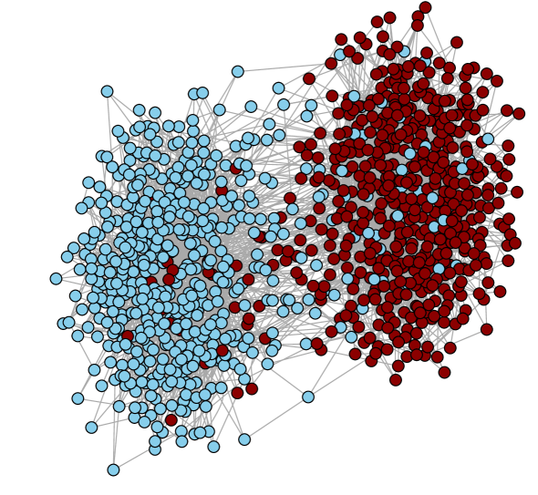
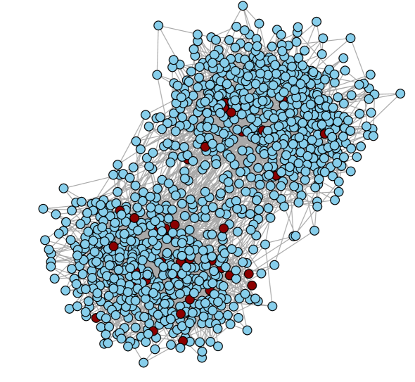
Figure 2: Examples of simulations with two weakly linked communities and $m=3,p_{0}=p_{1}=0,p_{2}=p_{3}=1$. In the left simulation different types are dominating in the two communities, with proportions of red vertices in the two communities being $0.877$ and $0.077$. In the right simulation blue appears to be dominating in both communities, with proportions of red vertices in the two communities being $0.057$ and $0.021$.

5.2 Symmetric community structure, random visible type

Here we consider the same community structure as in section 5.1 but the new vertex now picks one of the types it is exposed to uniformly at random. Hence $p_{0}=0$, $p_{1}=p_{2}=\frac{1}{2}$ and $p_{3}=1$, with $R(z)=\frac{3}{2}(z(1-z)^{2}+z^{2}(1-z))+z^{3}$, with a stable fixed point at $z=\frac{1}{2}$ and unstable fixed points at $z=0$ and $z=1$. In this case the results of [3] show that in standard preferential attachment the proportion of red tends to $\frac{1}{2}$ almost surely, and a corresponding result was shown to hold for any number of types and any $m\geq 3$ in [13]. This rule is increasing, and the only fixed points of $R(z)$ in $[0,1]$ are $z=0$, $z=1/2$ and $z=1$, with the first and last being linearly unstable ($R^{\prime}(0)=R^{\prime}(1)=3/2$). Consequently Theorem 3 shows that the same will apply for the multi community model, regardless of the community structure. Analysis of the stationary points in this case with community structure given by

$$A_{\theta}=\begin{pmatrix}1&\theta\\ \theta&1\end{pmatrix}$$

also appears in [19], again for $\mu_{1}=\mu_{2}=\frac{1}{2}$, and as might be expected from Theorem 3 the only stable stationary point is $(\frac{1}{4},\frac{1}{4},\frac{1}{4},\frac{1}{4})$, regardless of the value of $\theta$. So in this case there is no phase transition in $\theta$.

5.3 Only one possible limit with a single community, different limits in different communities

Theorem 4, part 2, implies that there are examples which that result applies to with the community structure given by

$$A=\begin{pmatrix}1&\theta\\ \theta&1\end{pmatrix},$$

but with $\theta>1$, indicating that vertices in fact prefer to connect to vertices in the other community. For example, consider this community structure with $\theta=10$, and take $m=3$ with the “minority rule”: the new vertex chooses to take the type which is less common among its neighbours, giving $p_{k}=1$ for $k=0,1$ and $p_{k}=0$ for $k=2,3$. Here $R(z)=(1-z)^{3}+3z(1-z)^{2}$ with a single, stable, fixed point at $z=\frac{1}{2}$, so for standard preferential attachment the proportion of red converges to $\frac{1}{2}$ almost surely. However, with the above community structure this rule is covered by part 2 of Theorem 4 and so shows positive probability of different limits in the two communities. An example of a simulation with 500 vertices and this rule appears in Figure 3, showing different types dominating in the two communities.

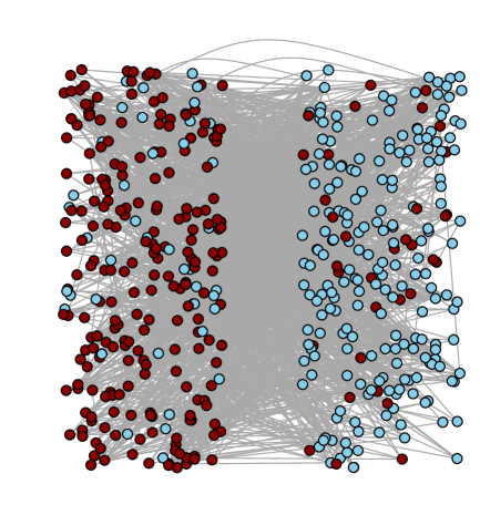
Figure 3: Example simulation showing different type dynamics in two communities in a case where a single community converges to the same limit. The left community has a proportion $0.840$ of its vertices being red, and the right community a proportion $0.151$ of its vertices being red.

5.4 Example with a touchpoint and an invisible community

We consider the rule with $m=3,p_{0}=1/4,p_{1}=0,p_{2}=p_{3}=1$; for this case $R(z)=\frac{1}{4}(1-z)^{3}+3z^{2}(1-z)+z^{3}$ and has a touchpoint at $z=\frac{1}{3}$ and a stable fixed point at $z=1$, so in the single community model the results of [3] will give both $\frac{1}{3}$ and $1$ as possible limits for the proportion of red vertices. Proposition 2 shows that if the community structure matrix $A$ has all entries positive then for small $\theta$ we do not get convergence to different limits here. However, if one community is invisible to the other this does not apply.

Consider an asymmetric community structure where, in the notation of Theorem 1

$$A_{\theta}=\begin{pmatrix}1&0\\ \theta&1\end{pmatrix},$$

with $\theta>0$, so that one community (the one labelled 1) is invisible to the other, but the other community is visible to both. We take $\mu_{1}=\frac{4}{5}$ and $\mu_{2}=\frac{1}{5}$, so that the invisible community is larger. Figure 4 shows an example of a simulation with the type assignment rule described in the last paragraph and this community structure; in this simulation the visible community is close to the touchpoint, but the invisible community is close to the stable root. Note that it intuitively makes sense that when the invisible community is relatively small it is likely to take the visible community’s type, but when it is larger, as here, it is easier for it to maintain its own type dynamics.

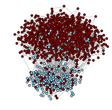
Figure 4: Here the larger invisible community has a proportion $0.923$ of its vertices red, while the smaller visible community has a proportion $0.269$ of its vertices red, suggesting that the latter may be converging to the touchpoint at $1/3$.

References

- [1] L. Addario-Berry, L. Devroye, G. Lugosi, and V. Velona. Broadcasting on random recursive trees. The Annals of Applied Probability, 32(1):497 – 528, 2022.
- [2] D. Aldous. Random partitions of the plane via poissonian coloring and a self-similar process of coalescing planar partitions. The Annals of Probability, 46(4):2000–2037, 2018.
- [3] T. Antunović, E. Mossel, and M. Rácz. Coexistence in preferential attachment networks. Combinatorics, Probability and Computing, 25:797–822, 2016.
- [4] A. Backhausz and B. Rozner. Asymptotic degree distribution in preferential attachment graph models with multiple type edges. Stoch. Models, 35(4):496–522, 2019.
- [5] M. Benaïm. Dynamics of stochastic approximation algorithms. Séminaire de Probabilités, XXXIII, 1709:1–68, 1999.
- [6] N. Berger, C. Borgs, J. Chayes, and A. Saberi. Asymptotic behaviour and distributional limits of preferential attachment graphs. Annals of Probability, 42:1–40, 2014.
- [7] G. Csardi and T. Nepusz. The igraph software package for complex network research. InterJournal, Complex Systems:1695, 2006.
- [8] P. Dai Pra, P.-Y. Louis, and I. G. Minelli. Synchronization via interacting reinforcement. Journal of Applied Probability, 51(2):556–568, 2014.
- [9] S. Dereich and T. Müller-Gronbach. General multilevel adaptations for stochastic approximation algorithms of Robbins–Monro and Polyak–Ruppert type. Numerische Mathematik, 142(2):279–328, 2019.
- [10] A. Flaxman, A. Frieze, and J. Vera. A geometric preferential attachment model of networks. Internet Math., 3:187–205, 2006.
- [11] A. Flaxman, A. Frieze, and J. Vera. A geometric preferential attachment model of networks II. Internet Math., 4:87–112, 2007.
- [12] B. Hajek and S. Sankagiri. Community recovery in a preferential attachment graph. IEEE Trans. Inform. Theory, 65(11):6853–6874, 2019.
- [13] J. Haslegrave and J. Jordan. Non-convergence of proportions of types in a preferential attachment graph with three co-existing types. Electronic Communications in Probability, 23:1–12, 2018.
- [14] J. Jordan. Geometric preferential attachment in non-uniform metric spaces. Electron. J. Probab, 18(8):1–15, 2013.
- [15] J. Jordan and A. Wade. Phase transitions for random geometric preferential attachment graphs. Advances in Applied Probability, 47:565–588, 2015.
- [16] S. Manna and P. Sen. Modulated scale-free network in Euclidean space. Phys. Rev. E, 66:066114, 2002.
- [17] R. Pemantle. A survey of random processes with reinforcement. Probability Surveys, 4:1–79, 2007.
- [18] K. Thulasiraman and M. N. S. Swamy. Graphs: theory and algorithms. A Wiley-Interscience Publication. John Wiley & Sons, Inc., New York, 1992.
- [19] M. Yarrow. A journey down the rabbit hole: pondering preferential attachment models with location. PhD thesis, University of Sheffield, 2019.