Gaussian Process Classification Bandits

Abstract

Classification bandits are multi-armed bandit problems whose task is to classify a given set of arms into either positive or negative class depending on whether the rate of the arms with the expected reward of at least $h$ is not less than $w$ for given thresholds $h$ and $w$. We study a special classification bandit problem in which arms correspond to points $x$ in $d$-dimensional real space with expected rewards $f(x)$ which are generated according to a Gaussian process prior. We develop a framework algorithm for the problem using various arm selection policies and propose policies called FCB and FTSV. We show a smaller sample complexity upper bound for FCB than that for the existing algorithm of the level set estimation, in which whether $f(x)$ is at least $h$ or not must be decided for every arm’s $x$. Arm selection policies depending on an estimated rate of arms with rewards of at least $h$ are also proposed and shown to improve empirical sample complexity. According to our experimental results, the rate-estimation versions of FCB and FTSV, together with that of the popular active learning policy that selects the point with the maximum variance, outperform other policies for synthetic functions, and the version of FTSV is also the best performer for our real-world dataset.

[H]organization=Graduate School of Information Science and Technology, Hokkaido University,addressline=
Kita 14, Nishi 9, Kita-ku, city=Sapporo, postcode=060-0814, state=Hokkaido, country=Japan

[R]organization=Research Institute for Electronic Science, Hokkaido University,addressline=
Kita 10, Nishi 8, Kita-ku, city=Sapporo, postcode=060-0810, state=Hokkaido, country=Japan

[O]organization=Department of Applied Physics, Osaka University,addressline=
2-1 Yamadaoka, city=Suita, postcode=565-0871, state=Osaka, country=Japan

[K]organization=Graduate School of Medical Science, Kyoto Prefectural University of Medicine,addressline=
465 Kajii-cho, city=Kamigyo-ku, postcode=602-8566, state=Kyoto, country=Japan

1 Introduction

Classification is a task that classifies a given instance into one of the pre-defined classes. Anomaly detection from image data can be seen as a classification task in which the data is classified into normal and anomaly. In some anomaly detection such as disease diagnoses, anomaly class can be defined by bad area ratio: the data is an anomaly if and only if the bad area ratio of the data is at least a certain threshold. In some cases like disease diagnoses by Raman spectra (Helal et al., 2019), we have to measure the badness of each point in a given region one by one instead of a one-shot measurement of the whole region. In this paper, we study the fast classification of a given region by its bad area ratio through measuring the badness of a point one by one iteratively.

Let a point $x$ in a given region of $d$-dimensional real space $\mathbb{R}^{d}$ be bad if and only if the badness $f(x)$ of $x$ is at least a given threshold, and assume that we can know noisy $f(x)$ by measuring at point $x$. We also assume that the bad area ratio can be approximated by the bad point ratio in the finite point set $D$ that is composed of (coarsely) quantized points in the given bounded region $X\subset\mathbb{R}^{d}$. To introduce correlation between $f(x)$ of different points, $f(x)$ for all $x\in D$ are assumed to be generated by the Gaussian process prior with mean $0$ and some appropriate kernel. Correlation brought by the Gaussian process assumption makes correct judgment possible with high probability by measuring only at a part of the whole point set. The level set estimation problem studied by Gotovos et al. (2013) is a problem of this setting though the objective is the discrimination of whether each point in the whole set is bad or not. In our classification setting, we do not have to know the badness of every point in the whole set to judge whether the bad area ratio is at least a given threshold or not, and thus an earlier stopping time can be realized.

Since we only consider a finite point set $D$ in a given region, the problem we deal with here is just a multi-armed classification bandit problem studied by Tabata et al. (2021). In the paper, however, no correlation between arms’ rewards is assumed. By making use of the correlation between points’ rewards in our problem setting, a reduction of the sample complexity can be expected. The result of our experiment using a real-world dataset shows the effectiveness of using the correlation between points’ rewards.

We propose Algorithm GPCB[ASP] (Gaussian Process Classification Bandits [Arm Selection Policy]), in which any arm selection policy function ASP can be used. We prove the correctness of GPCB[ASP] for any ASP as a solution for our PAC-like problem: for given $\delta,\varepsilon>0$ and given thresholds $h,w$, decide whether the rate of points with badness at least $h+\varepsilon$ is at least $w$ or the rate of points with badness less than $h-\varepsilon$ is more than $1-w$, correctly with probability at least $1-\delta$ when one of them is true. For the PAC-like problem, we show a high-probability sample complexity upper bound $C/(\Delta_{w}+\varepsilon)^{2+o(1)}$ of GPCB[FCB] using a specific ASP called FCB (Farthest Confidence Bound), where $C$ is a constant value that depends on the dimension $d$ and the adopted kernel in Gaussian process, and $\Delta_{w}$ is the difference between $\lceil w|D|\rceil$th largest badness value $f(x)$ $(x\in D)$ and threshold $h$. This upper bound is smaller than the sample complexity upper bound $C/(2\varepsilon)^{2+o(1)}$ of the LSE algorithm for the harder level set estimation problem in the case with $\Delta_{w}>\varepsilon$. Furthermore, we prove that GPCB[ASP] which is modified for the level set estimation and uses an ASP of always selecting an uncertain arm, achieves the same sample complexity upper bound $C/(2\varepsilon)^{2+o(1)}$ as the LSE algorithm, which implies the same sample complexity upper bound of GPCB[ASP] for the easier classification bandits. As arm selection policy functions, we also propose rate estimation versions of ASPs that use the estimation $\hat{r}$ of rate $|H_{h}|/|D|$, and narrow the candidates to $\tilde{H}$ if $\hat{r}\geq w$ and $D\setminus\tilde{H}$ otherwise, where $H_{h}$ is a set of points whose badness is at least $h$, and $\tilde{H}$ is the estimated set of $H_{h}$.

We check empirical sample complexities of GPCB[ASP] for various ASPs, including their rate estimation versions using two types of synthetic functions (GP-prior-generated functions and benchmark functions) and a real-world dataset. For synthetic functions, GPCB[ASP]s with ASP$=$FCB and FTSV (Farthest Thompson Sampling Value) outperform those with LSE (Level Set Estimation) (Gotovos et al., 2013) and STR (STRaddle heuristic) (Bryan et al., 2006), where LSE and STR are state-of-the-art arm selection policies used for the level set estimation. Performance of the rate estimation version ASP${}_{\text{RE}}$ of an ASP significantly improves for FCB, FTSV, and VAR (VARiance), where VAR is a popular active learning policy that selects the point with the maximum variance. As a result, GPCB[FCB${}_{\text{RE}}$], GPCB[FTSV${}_{\text{RE}}$], and GPCB[VAR${}_{\text{RE}}$] are the best performers for both types of synthetic functions. As the real-world dataset, we use cancer index images that are made from Raman images of cancer and non-cancer thyroid follicular cells. Our algorithm GPCB[ASP] correctly classifies all nine images into cancer and non-cancer ones by iteratively asking cancer indices of less than 0.95% points for all the ASPs we used. In contrast, cancer indices of at least 1.6% points are required for the existing classification bandit algorithm (Tabata et al., 2021). GPCB[FTSV${}_{\text{RE}}$] is the best performer for this real-world dataset.

Related Work

This research is categorized into stochastic bandit problem (Auer et al., 2002) of pure exploration (Bubeck et al., 2009) with fixed confidence setting (Even-Dar et al., 2002). Both exploration and exploitation are needed for the objective of cumulative reward maximization, but exploration only is needed in the case that algorithms are evaluated by their final outputs only, and such kinds of problems are called pure exploration problems. The most popular pure exploration bandit problem is the best arm identification (Audibert et al., 2010), and there is its variation that identifies all the above-threshold arms, that is, the arms with a mean reward more than a given threshold (Locatelli et al., 2016; Kano et al., 2019). For a given reward threshold, instead of identifying all the above-threshold arms, the decision bandit problem of whether or not an above-threshold arm exists, was studied in (Kaufmann et al., 2018; Tabata et al., 2020). Recently, an extended decision bandit problem called classification bandits has been proposed (Tabata et al., 2021). In classification bandits, a threshold on the number of above-threshold arms is introduced, and the problem is to decide whether the number of above-threshold arms in a given set of arms is more than the introduced threshold or not. Classification bandit problem can be seen as a kind of more general active sequential hypothesis testing problem, which was studied and nice theoretical analyses were provided by Degenne and Koolen (2019); Garivier and Kaufmann (2021). In this paper, we study the classification bandit problem with finite arms that correspond to points in $\mathbb{R}^{d}$ with correlated rewards depending on their positions.

In the context of active learning, the problem of level set estimation is studied. The level set estimation is a problem to determine whether an unknown function value at $x$ is above or below some given threshold for all the points $x$ in a given set $D\in\mathbb{R}^{d}$ by iteratively asking noisy function values. In (Bryan et al., 2006; Gotovos et al., 2013), the Gaussian process prior is used as a correlation assumption for function values, and Gotovos et al. (2013) proved the sample complexity upper bound of their proposed algorithm LSE and reported the F1-scores of LSE and STR better than that of VAR (VARiance), where STR is a straddle heuristic proposed by Bryan et al. (2006) and VAR is a popular active learning method that selects the maximum variance points. The problem we deal with can be seen as an easier variation of the level set estimation in which it is only checked whether the rate of points with above-threshold function value is above a given threshold or not. We prove a better sample complexity upper bound for this variation.

2 Problem Settings

For a bounded set $X\subset\mathbb{R}^{d}$, assume the existence of an unknown function $f:X\to\mathbb{R}$. What we want to know is whether the ratio of the area $f(x)\geq h$ is at least $w$ or not for given two thresholds $h,w\in\mathbb{R}$. Here, we assume that the ratio can be approximately estimated by the ratio of those in a finite set $D$ of points in $X$, and formulate the problem for $D\subset X\subset\mathbb{R}^{d}$. Observable information for answering the question is noisy function values $y=f(x)+\eta$ for requested points $x\in D$, where $\eta\in\mathbb{R}$ is assumed to be generated according to a normal distribution $N(0,\sigma^{2})$. Our objective is to answer the question correctly with high probability by asking as a small number of noisy function values as possible. In this setting, it is difficult to correctly answer whether $f(x)\geq h$ or not for the point $x$ whose function value is close to the threshold $h$. Thus, by introducing a margin $\varepsilon$, we consider the problem of whether the ratio of the area $f(x)\geq h+\varepsilon$ is at least $w$ or not. We formally define this problem as follows.

Problem 1 (Classification Bandits with Margin $\epsilon$).

Given $\varepsilon>0$ and $\delta>0$, output “positive” with probability at least $1-\delta$ if $|H_{h+\varepsilon}|/|D|\geq w$ and output “negative” if $|L_{h-\varepsilon}|/|D|>1-w$ by asking as small number of noisy function values of $f$ as possible, where $H_{h+\varepsilon}=\{x\in D\mid f(x)\geq h+\varepsilon\}$, $L_{h-\varepsilon}=\{x\in D\mid f(x)<h-\varepsilon\}$, and $|\cdot|$ denotes the number of elements in a set ‘$\cdot$’.

Note that any output with any probability is allowed when $|H_{h+\varepsilon}|/|D|<w$ and $|L_{h-\varepsilon}|/|D|\leq 1-w$.

This bandit problem is a pure exploration problem like the best arm identification. This problem can be seen as a classification problem in which a set $D$ with a function $f$ is classified into “positive” or “negative”. Thus, this kind of bandit problem is called classification bandits (Tabata et al., 2021). In this paper, we develop faster classification algorithms by assuming a correlation between $f(x)$ of points in $D\subset X$.

As the level set estimation that Gotovos et al. (2013) studied, we assume that target function values $f(x)\in D$ are generated from a Gaussian process (GP), that is, a target function $f(\cdot)$ over $D$ is drawn according to $\mathrm{GP}(\mu(\cdot),k(\cdot,\cdot))$ with $\mu(x)=0$ for $x\in D$ and some kernel function $k(\cdot,\cdot)$. Throughout this paper, we assume $k(x,x^{\prime})\leq 1$ for $x,x^{\prime}\in D$. Given a list of $t$ noisy observations $\mathbf{y}_{t}=(y_{1},\dots,y_{t})^{\mathsf{T}}$ for a list of $t$ inputs $(x_{1},\dots,x_{t})$, the posterior of $f(\cdot)$ is $\mathrm{GP}(\mu_{t}(\cdot),k_{t}(\cdot,\cdot))$ with $\mu_{t}$ and $k_{t}$ calculated as follows:

$$\mu_{t}(x) ={\mathbf{k}}_{t}(x)^{\mathsf{T}}({\mathbf{K}}_{t}+\sigma^{2}{\mathbf{I}})^{-1}\mathbf{y}_{t},$$ (1)

$$k_{t}(x,x^{\prime}) =k(x,x^{\prime})-{\mathbf{k}}_{t}(x)^{T}({\mathbf{K}}_{t}+\sigma^{2}{\mathbf{I}})^{-1}{\mathbf{k}}_{t}(x),\text{ and}$$ (2)

$$\sigma_{t}^{2}(x) =k_{t}(x,x),$$ (3)

where ${\mathbf{k}}_{t}(x)=[k(x_{1},x),\dots,k(x_{t},x)]^{\mathsf{T}}$ and ${\mathbf{K}}_{t}=[\mathbf{k}_{t}(x_{1}),\dots,\mathbf{k}_{t}(x_{t})]$. What we call Gaussian process classification bandits is Problem 1 with this Gaussian process assumption.

The Gaussian process classification bandit problem is a problem easier than the level set estimation; in level set estimation, all the points in $H_{h+\varepsilon}\cup L_{h-\varepsilon}$ must be identified correctly with probability at least $1-\delta$, from which the answer of Problem 1 can be derived. For this easier problem, we show arm selection policies with smaller sample complexities theoretically and empirically.

3 Proposed Method

3.1 Algorithm GPCB[ASP]

Algorithm 1 GPCB[$\mathrm{ASP}$] ($D,k,\varepsilon,\delta,h,w$)

0:  $\mathrm{ASP}$: Arm Selection Policy

0:   $D$: samplable point set, $k$: kernel of the GP prior, $\varepsilon$: accuracy parameter, $\delta$: confidence parameter, $h$: function value threshold, $w$: high-value ratio threshold

0:  $\beta_{t}=2\log(|D|\pi^{2}t^{2}/6\delta)$

0:  “positive” or “negative”

1:  $\hat{H}\leftarrow\phi,\hat{L}\leftarrow\phi,U_{0}\leftarrow D$

2:  $C_{0}(x)\leftarrow(-\infty,\infty),\mu_{0}(\cdot)\leftarrow 0,k_{0}(\cdot,\cdot)\leftarrow k(\cdot,\cdot)$

3:  $t\leftarrow 1$

4:  while $U_{t-1}\neq\phi$ do

5:     $U_{t}\leftarrow\emptyset$

6:     for all $x\in U_{t-1}$ do

7:        $C_{t}(x)\leftarrow C_{t-1}(x)\cap[\mu_{t-1}(x)-\sqrt{\beta_{t}}\sigma_{t-1}(x),\mu_{t-1}(x)\!+\!\sqrt{\beta_{t}}\sigma_{t-1}(x)]$

8:        if $\min(C_{t}(x))\geq h-\varepsilon$ then

9:           $\hat{H}\leftarrow\hat{H}\cup\{x\}$

10:        else if $\max(C_{t}(x))<h+\varepsilon$ then

11:           $\hat{L}\leftarrow\hat{L}\cup\{x\}$

12:        else

13:           $U_{t}\leftarrow U_{t}\cup\{x\}$

14:        end if

15:     end for

16:     if $|\hat{H}|/|D|\geq w$ then

17:        return  “positive”

18:     else if $|\hat{L}|/|D|>1-w$ then

19:        return  “negative”

20:     end if

21:     $x_{t}\leftarrow\mathrm{ASP}(U_{t},C_{t},\mu_{t-1},k_{t-1},h)$

22:     Ask $f(x_{t})$ and receive its noisy value $y_{t}$

23:     Calculate $\mu_{t}$ and $k_{t}$ using Eqs. (1) and (2)

24:     $t\leftarrow t+1$

25:  end while

For Gaussian process classification bandits, we propose an algorithm GPCB[ASP] (Gaussian Process Classification Bandits [Arm Selection Policy]) using any arm selection policy function ASP, which is shown in Algorithm 1. Function ASP, which is used in Line 21, selects the point $x_{t}\in D$ to ask its noisy function value $y_{t}$ at time step $t$. GPCB[ASP] maintains a high-probability confidence interval $C_{t}(x)$ for each point $x\in D$ at each time step $t$ and puts $x$ into the estimated high-value point set $\hat{H}$ if $\min C_{t}\geq h-\varepsilon$ (Line 9), into the estimated low-value point set $\hat{L}$ if $\max C_{t}<h+\varepsilon$ (Line 11), and into the uncertain point set $U_{t}$ otherwise (Line 13). GPCB[ASP] stops when $|\hat{H}|/|D|\geq w$ or $|\hat{L}|/|D|>1-w$ holds, and outputs “positive” in the former case and “negative” in the latter case.

Differences from the LSE algorithm (Gotovos et al., 2013) are the following two points:(1) in addition to condition $U_{t-1}=\emptyset$, two other stopping conditions $|\hat{H}|/|D|\geq w$ and $|\hat{L}|/|D|>1-w$ are checked for the realization of earlier stopping time in our easier problem setting, (2) any ASP can be used instead of fixing as ASP$=$LSE.

As the LSE algorithm (Gotovos et al., 2013) for the level set estimation, we adopt

$$C_{t}(x)=\bigcap_{i=1}^{t}[\mu_{i-1}(x)-\sqrt{\beta_{i}}\sigma_{i-1}(x),\mu_{i-1}(x)+\sqrt{\beta_{i}}\sigma_{i-1}(x)]$$ (4)

as the confidence interval $C_{t}(x)$ for the GP posterior $\mathrm{GP}(\mu_{t}(\cdot),k_{t}(\cdot,\cdot))$ using the GP prior $\mathrm{GP}(0,k(\cdot,\cdot))$, where $\beta_{t}$, $\mu_{0}(x)$ and $\sigma_{0}(x)$ are set as $\beta_{t}=2\log(|D|\pi^{2}t^{2}/6\delta)$, $\mu_{0}(x)=0$ and $\sigma_{0}(x)=\sqrt{k(x,x)}$.

Using confidence intervals $C_{t}(x)$ defined by Eq. (4), the following corollary is known to hold. The corollary leads to Theorem 1 which guarantees the correct output of GPCB[ASP] for any arm selection policy if it terminates.

Corollary 1 (Corollary 1 in (Gotovos et al., 2013)).

Let $\beta_{t}=2\log(|D|\pi^{2}t^{2}/6\delta)$ for $\delta\in(0,1)$ and $t\geq 1$. Then,

$$f(x)\in C_{t}(x)\text{\ for all $x\in D$ and $t\geq 1$}$$

holds with probability at least $1-\delta$.

Theorem 1.

For any $h\in\mathbb{R},w,\delta\in(0,1),\epsilon>0$, if algorithm GPCB[ASP] terminates, it outputs “positive” with probability at least $1-\delta$ in the case with $|H_{h+\epsilon}|/|D|\geq w$, and “negative” with probability at least $1-\delta$ in the case with $|L_{h-\epsilon}|/|D|>1-w$.

Proof.

If GPCB[ASP] terminates at time $t$, $|\hat{H}|/|D|\geq w$ or $|\hat{L}|/|D|>1-w$ must hold at time $t$ because $(|\hat{H}|+|\hat{L}|)/|D|<1$ holds otherwise, which implies $U_{t}\neq\emptyset$ that contradicts the fact GPCB[ASP] terminates at time $t$. Thus, whenever GPCB[ASP] terminates, it outputs “positive” or “negative”. Let $t$ be the stopping time.

For $C_{t}(x)$ defined by Eq. (4), by Corollary 1,

$$f(x)\in C_{t}(x)\text{ for any }x\in D\text{ and }t\geq 1$$ (5)

holds with probability at least $1-\delta$. If (5) holds, GPCB[ASP] never outputs “negative” in the case with $|H_{h+\epsilon}|/|D|\geq w$ because, for all $x\in H_{h+\epsilon}$ and $t\geq 1$, $\max(C_{t}(x))\geq f(x)\geq h+\varepsilon$ holds, and thus $x\not\in\hat{L}$. Thus, GPCB[ASP] always outputs “positive” in this case if it terminates. We can similarly prove the theorem statement in the case with $|L_{h-\epsilon}|/|D|>1-w$. ∎

3.2 Arm Selection Policies for Algorithm GPCB

We consider three arm selection policy functions, FCB, LSE, and FTSV. In each of them, we define value $a_{t}(x)$ for each point $x\in U_{t}$ and $t\geq 1$, which indicates how good the point $x$ is as the next point to ask its noisy function value of $f(x)$. Using different $a_{t}(x)$, each of them selects $x\in U_{t}$ with the maximum $a_{t}(x)$ as the next query point $x_{t}$, that is,

$$\text{ASP}(U_{t},C_{t},\mu_{t-1},k_{t-1},h)=\mathop{\rm argmax}\limits_{x\in U_{t}}a_{t}(x).$$ (6)

The definitions of $a_{t}(x)$ for each arm selection policy function ASP are as follows:

FCB

(Farthest Confidence Bound)

$$a_{t}(x)=\max\{\max(C_{t}(x))-h,h-\min(C_{t}(x))\}$$

LSE

(Level Set Estimation (Gotovos et al., 2013))

$$a_{t}(x)=\min\{\max(C_{t}(x))-h,h-\min(C_{t}(x))\}$$

FTSV

(Farthest Thompson Sampling Value)

$$a_{t}(x)=|g_{t}(x)-h|\text{ for }g_{t}\sim\mathrm{GP}(\mu_{t-1},k_{t-1})$$

Algorithm GPCB[ASP] should select a point $x_{t}$ that promotes the growth of the estimated high-value point set $\hat{H}$ if the “positive” possibility is high and promotes the growth of the estimated low-value point set $\hat{L}$ otherwise. Incorporating this idea to the arm selection policies, we also propose their rate estimation versions FCB${}_{\text{RE}}$, LSE${}_{\text{RE}}$, and FTSV${}_{\text{RE}}$ as follows:

$$\text{ASP}(U_{t},C_{t},\mu_{t-1},k_{t-1},h)=\begin{cases}\mathop{\rm argmax}\limits_{x\in\tilde{H}_{t}}a_{t}(x)&\text{ if }|\hat{H}\cup\tilde{H}_{t}|/|D|\geq w\\ \mathop{\rm argmax}\limits_{x\in U_{t}\setminus\tilde{H}_{t}}a_{t}(x)&\text{ otherwise, }\end{cases}$$ (7)

where $\tilde{H}_{t}$ is defined as

$$\tilde{H}_{t}=\begin{cases}\{x\in U_{t}\mid\max(C_{t}(x))-h\geq h-\min(C_{t}(x))\}&\text{ (FCB${}_{\text{RE}}$, LSE${}_{\text{RE}}$)}\\ \{x\in U_{t}\mid g_{t}(x)\geq h\}&\text{ (FTSV${}_{\text{RE}}$).}\end{cases}$$

3.3 Sample Complexity Upper Bounds

This section first shows a sample complexity upper bound of algorithm GPCB[ASP] for any arm selection policy ASP that always selects a point $x\in U_{t}$. Then we also show a high-probability sample complexity upper bound of algorithm GPCB[FCB] that is better than it for problem instances with some moderate complexity.

As the sample complexity upper bound of Algorithm LSE for the level set estimation in (Gotovos et al., 2013), those sample complexity upper bounds can be derived by lower and upper bounding the information gain $I(\mathbf{y}_{t};\mathbf{f}_{t})$ from a list of noisy function values $\mathbf{y}_{t}=(y_{1},\dots,y_{t})^{\mathsf{T}}$ for a list of target function values $\mathbf{f}_{t}=(f(x_{1}),\dots,f(x_{t}))^{\mathsf{T}}$ of $\mathbf{x}_{t}=(x_{1},\dots,x_{t})^{\mathsf{T}}$. Information gain $I(\mathbf{y}_{t};\mathbf{f}_{t})$ is defined as

$$I(\mathbf{y}_{t};\mathbf{f}_{t})=H(\mathbf{y}_{t})-H(\mathbf{y}_{t}\mid\mathbf{f}_{t}).$$

Define $\gamma_{t}$ as

$$\gamma_{t}=\max_{\mathbf{x_{t}}\in D}I(\mathbf{y}_{t};\mathbf{f}_{t}).$$

Then, $I(\mathbf{y}_{t};\mathbf{f}_{t})$ is upper bounded by $\gamma_{t}$, and its increasing order is known to be $\gamma_{t}=O(d\log t)$ for linear kernel $k(x,x^{\prime})=x^{\mathsf{T}}x^{\prime}$, $\gamma_{t}=O((\log t)^{d+1})$ for the squared exponential kernel $e^{-\frac{||x-x^{\prime}||^{2}}{2\ell}}$ with length scale parameter $\ell$, where $x,x^{\prime}\in D\subset\mathbb{R}^{d}$ (Srinivas et al., 2012).

As a complexity measure of problem instances, we use $\Delta_{w}$ which is defined as

$$\Delta_{w}=|f(x^{(\lceil w|D|\rceil)})-h|,$$

where $x^{(i)}$ is the point that has the $i$-th largest function value in $D$. The complexity of the problem increases as $\Delta_{w}$ becomes smaller. We evaluate sample complexity upper bound in the form of $T(\cdot)$, where function $T(\Delta)$ is defined as

$$T(\Delta)=\min\left\{t\in\mathbb{N}\left|\ \frac{t}{\beta_{t}\gamma_{t}}>\frac{C_{1}}{\Delta^{2}}\right.\right\}.$$

Here $C_{1}=8/\log(1+\sigma^{-2})$. Note that this function $T(\Delta)$ is a nonincreasing function, and thus $T(\Delta)$ for the larger $\Delta$ is better as sample complexity. We know $T(\Delta)<\frac{C}{\Delta^{2+o(1)}}$ for some constant $C$ that depends on $|D|$, $\delta$, $d$ and $\sigma$. (See A.) Furthermore, we can also derive $T(\Delta)<\left(\frac{C^{\prime}d}{\Delta^{2}}\right)^{1+o(1)}$ for the linear kernel and $T(\Delta)<\left(\frac{C^{\prime\prime}(d+2)^{(d+2)}}{\Delta^{2}}\right)^{1+o(1)}$ for the squared exponential kernel for some constants $C^{\prime}$ and $C^{\prime\prime}$ that depend on $|D|$, $\delta$, and $\sigma^{2}$.

The sample complexity of Algorithm GPCB[ASP] for any arm selection policy function ASP that always selects $x$ from the uncertain point set $U_{t}$ at time $t$ is upper bounded by $T(2\varepsilon)$ by the following theorem.

Theorem 2.

For any $h\in\mathbb{R},w,\delta\in(0,1)$, $\epsilon>0$, and for any arm selection policy function ASP that selects $x\in U_{t}$ at any time $t$, Algorithm GPCB[ASP] always terminates after receiving at most $T(2\epsilon)$ function values.

Proof.

See B. ∎

The proof of Theorem 2 is a simplified refinement of that of Theorem 1 in (Gotovos et al., 2013), and takes the stopping condition $U_{t}=\emptyset$ only into account. Thus the sample complexity bound $T(2\epsilon)$ holds even for the modified GPCB in which checking of additional two conditions (Line 16-20) is removed. This fact means that, though Gotovos et al. (2013) proved the sample complexity bound $T(2\epsilon)$ for the arm selection policy LSE only, the same bound $T(2\epsilon)$ can be proved for any arm selection policy that selects $x\in U_{t}$ at any time $t$ in the problem of level set estimation.

When $\Delta_{w}>\varepsilon$, we can prove better sample complexity bound $T(\Delta_{w}+\varepsilon)$ depending on our problem setting for Algorithm GPCB[FCB] as the following theorem.

Theorem 3.

For any $h\in\mathbb{R},w,\delta\in(0,1)$ and $\epsilon>0$, Algorithm GPCB[FCB] terminates after receiving at most $T(\Delta_{w}+\epsilon)$ noisy function values with probability at least $1-\delta$.

Proof.

See C. ∎

4 Experiments

In this section, we compare the experimental performance of Algorithm GPCB[ASP] for various ASPs and their rate estimation versions using synthetic functions and real-world data. In all the result tables, the best numbers are bolded, and the numbers that are not significantly different from them are italicized.

4.1 Comparison Algorithms

In addition to ASP$=$FCB, LSE, FTSV, and their rate estimation versions, we compare their performances of GPCB[ASP] with those of the following existing ASPs, which also select $x_{t}$ by Eq. (6) using $a_{t}(x)$ defined as:

UCB

(Upper Confidence Bound)

$$a_{t}(x)=\mu_{t-1}(x)+\sqrt{\beta_{t}}\sigma_{t-1}$$

LCB

(Lower Confidence Bound)

$$a_{t}(x)=\mu_{t-1}(x)-\sqrt{\beta_{t}}\sigma_{t-1}$$

TS

(Thompson Sampling)

$$a_{t}(x)=g_{t}(x)\text{ for }g_{t}\sim\mathrm{GP}(\mu_{t-1},k_{t-1})$$

VAR

(VARiance)

$$a_{t}(x)=\sigma_{t-1}^{2}(x)=k_{t-1}(x,x)$$

STR

(STRaddle heuristic (Bryan et al., 2006))

$$a_{t}(x)=1.96\sigma_{t-1}(x)-|\mu_{t-1}(x)-h|$$

The rate estimation versions VAR${}_{\text{RE}}$ and STR${}_{\text{RE}}$ of VAR and STR, respectively, select $x_{t}$ by Eq. (7) using $\tilde{H}_{t}$ defined as

$$\tilde{H}_{t}=\{x\in U_{t}\mid\mu_{t-1}(x)\geq h\}.$$

For every algorithm, we set $\sqrt{\beta_{t}}=3$ as in the experiments by Gotovos et al. (2013). The dimensions $d$ of all the datasets are two. We use Gaussian kernel $k(x,x^{\prime})=\sigma^{2}_{kernel}\exp(\|x-x^{\prime}\|^{2}/2l^{2})$ with parameters $\sigma^{2}_{kernel}$ and $l$ in all the experiments. In all the experiments except that using GP-prior-geneated functions, we tune kernel parameters by maximum likelihood estimation for 100 samples generated from a uniform distribution.

4.2 Synthetic Functions

We conduct numerical experiments using two types of synthetic functions. One is a type of function generated according to a GP prior and the other is a type of function used as a benchmark. In all the experiments using synthetic functions, domain $D$ is set to $[a,a+b]^{2}$ for some $a,b\in\mathbb{R}$, and $D$ is defined as $D=\{(a+ib/30,a+jb/30)\mid i,j=0,1,\dots,30\}$. Note that $|D|=961$.

4.2.1 GP-Prior-Generated Functions

Table 1: #(function values) asked by GPCB[ASP] for ASPs without rate estimations. The numbers are averaged over 100 functions generated from $\mathrm{GP}(0,k(x,x^{\prime}))$ and their 95% confidence intervals are also shown. The underlined bolded numbers are the best among those for all the ASPs in Tables 1 and 2.

ASP	$w=0.2$		$w=0.4$		$w=0.6$		$w=0.8$
FCB	71.94$\pm$	2.17	180.5$\pm$	7.9	184.0$\pm$	7.9	72.04$\pm$	1.87
LSE	72.09$\pm$	1.76	199.0$\pm$	16.6	202.4$\pm$	15.9	71.70$\pm$	1.50
FTSV	72.95$\pm$	2.16	185.2$\pm$	9.6	188.1$\pm$	7.9	72.53$\pm$	1.99
STR	73.00$\pm$	0.55	261.5$\pm$	2.9	386.0$\pm$	26.9	84.00$\pm$	1.94
VAR	64.00$\pm$	0.83	174.0$\pm$	10.3	216.0$\pm$	4.4	79.00$\pm$	1.66
TS	57.58$\pm$	1.75	159.3$\pm$	7.4	337.3$\pm$	18.0	112.20$\pm$	2.67
UCB	58.50$\pm$	0.42	180.0$\pm$	3.1	451.0$\pm$	23.0	112.00$\pm$	1.11
LCB	101.44$\pm$	2.41	301.5$\pm$	21.6	155.1$\pm$	6.4	55.83$\pm$	1.62

growth curve of $|\hat{H}|/|D|$	growth curve of $|\hat{L}|/|D|$

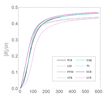
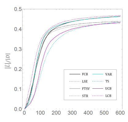
Figure 1: Growth curves of $|\hat{H}|/|D|$ (left) and $|\hat{L}|/|D|$ (right) averaged over $100$ simulations for Algorithm GPCB[ASP] with ASPs without rate estimations. The horizontal axis shows the number of observed function values.

We generate target functions $f$ by sampling from the GP prior $\mathrm{GP}(0,k(x,x^{\prime}))$ that is assumed in our problem settings. Domain $X$ is defined as $X=[-1,1]^{2}$. The parameters $\sigma_{kernel}$ and $l$ of the Gaussian kernel are set as $\sigma_{kernel}=1$, $l=0.2$. Values $\varepsilon=10^{-8},\sigma=0.1$ are used, and $h$ is set so that $|H_{h}|/|D|=0.5$ holds in this experiment.

The average numbers of function values asked by GPCB[ASP] and their 95% confidence intervals for ASPs without rate estimations are shown in Table 1. Note that the result is averaged over 100 functions generated according to $\mathrm{GP}(0,k(x,x^{\prime}))$. TS and UCB perform well when the true answer is positive but perform poorly in the other case as a result of always selecting the estimated highest point. LCB performs oppositely as a result of always selecting the estimated lowest point. These characteristics of TS, UCB, and LCB can be confirmed by the growth curves of $|\hat{H}|/|D|$ and $|\hat{L}|/|D|$ over the number of asked function values (Figure 1). FCB and VAR look the best performers, FTSV performs the next, and LSE follows. STR does not perform well when $w$ is close to the high-value point rate, and LSE has a similar tendency. The reason why VAR performs well without using threshold $h$ in its calculation, is guessed as that VAR’s selection resembles FCB’s selection in the GPCB framework, in which all the ASP selects a query point from $U_{t}$ excluding $\hat{H}$ and $\hat{L}$.

Table 2: #(function values) asked by GPCB[ASP] for ASPs with rate estimations. The meanings of the shown numbers are the same as in Table 1.

ASP	$w=0.2$		$w=0.4$		$w=0.6$		$w=0.8$
FCB${}_{\text{RE}}$	54.63$\pm$	1.64	158.6$\pm$	8.8	159.6$\pm$	7.7	54.32$\pm$	1.45
LSE${}_{\text{RE}}$	62.16$\pm$	2.05	216.3$\pm$	27.3	222.6$\pm$	42.5	63.33$\pm$	1.99
FTSV${}_{\text{RE}}$	56.53$\pm$	1.71	160.8$\pm$	7.8	166.3$\pm$	7.9	56.53$\pm$	1.60
STR${}_{\text{RE}}$	68.47$\pm$	7.83	337.8$\pm$	72.6	325.9$\pm$	49.6	71.10$\pm$	13.80
VAR${}_{\text{RE}}$	56.96$\pm$	1.47	149.1$\pm$	8.1	158.4$\pm$	10.9	56.88$\pm$	1.89

growth curve over $|\hat{H}|/|D|$	growth curve over $|\hat{L}|/|D|$

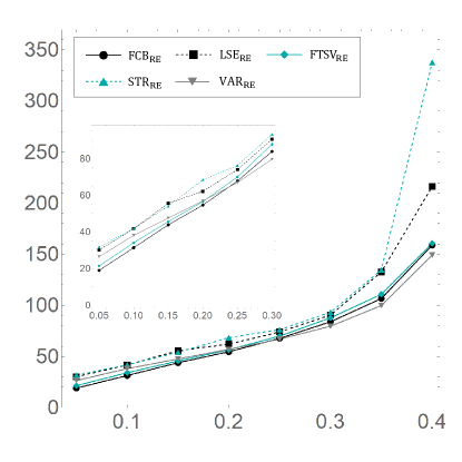
Figure 2: Growth curves of #(function values) over $|\hat{H}|/|D|$ (left) and $|\hat{L}|/|D|$ (right) for Algorithm GPCB[ASP] with rate estimation versions of ASPs . Each value is averaged over $100$ simulations. The inside plot shows a zoomed portion of a plot from $0.05$ to $0.30$.

growth curve of $|\hat{H}|/|D|$	growth curve of $|\hat{L}|/|D|$

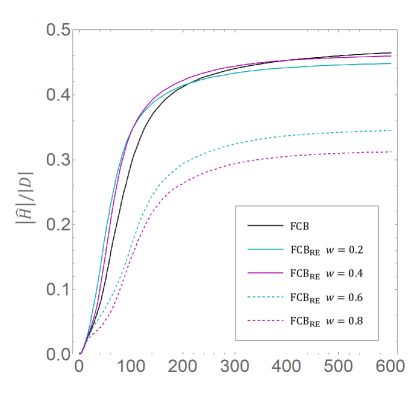
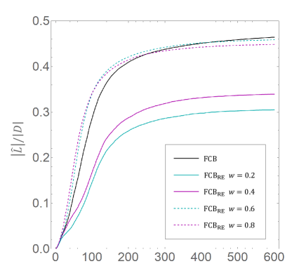
Figure 3: Growth curves of $|\hat{H}|/|D|$ (left) and $|\hat{L}|/|D|$ (right) averaged over $100$ simulations for Algorithm GPCB[ASP] with ASP=FCB and FCB${}_{\text{RE}}$. The horizontal axis shows the number of function values.

The results for ASPs with rate estimations are shown in Table 2. Rate estimations reduce the number of function values asked by GPCB[ASP] by about 20% on average for FCB, VAR, and FTSV while not always reducing that for LSE and STR. LSE and STR are algorithms for level set estimation whose task is to determine belonging for every point in $D$, and thus a point $x$ with $f(x)$ close to $h$ is preferred to be asked in some cases to achieve the task efficiently. Growth curves of the number of asked function values over $|\hat{H}|/|D|$ and $|\hat{L}|/|D|$ in Figure 2 indicate similar behaviors of FCB and FTSV. From the curves, we know that FCB and FTSV perform better than VAR for the thresholds $w$ that are far from the real rate $|H_{h}|/|D|=0.5$ while VAR performs a little bit better for thresholds $w$ that are close to the real rate. Growth curves of $|\hat{H}|/|D|$ and $|\hat{L}|/|D|$ for ASP=FCB and FCB${}_{\text{RE}}$ with various $w$ are shown in Figure 3. We can see that the setting value of $w$ changes the algorithm’s priority on which points in $\hat{H}$ or $\hat{L}$ should be found.

4.2.2 Benchmark Functions

In the experiments using two benchmark functions, we compare empirical sample complexities of GPCB[ASP] with ASPs that are good performers for GP-prior-generated functions: FCB, LSE, FTSV, VAR, and their rate estimation versions. Among them, we omit the result for FTSV because its performance was observed to be always similar to (or a little bit worse than) FCB’s performance.

Gauss Function

The first benchmark function is the two-dimensional Gaussian function $f(x,y)=5e^{-3(x^{2}+y^{2})}$ for $(x,y)\in X=[-1,1]^{2}$. We set $\varepsilon=10^{-8},\sigma=0.1$, and $h=0.5$. In this setting, $|H_{h}|/|D|=0.567118$. The tuned Gaussian kernel parameters $\sigma_{kernel}$ and $l$ are $1.29$ and $0.53$, respectively.

Table 3: #values of the two-dimensional Gaussian function asked by GPCB[ASP] averaged over ten simulations and its 95% confidence interval for various ASPs.

ASP	$w=0.2$		$w=0.4$		$w=0.6$		$w=0.8$
FCB	10.9$\pm$	0.92	24.4$\pm$	1.82	261.0$\pm$	45.6	33.3$\pm$	1.07
LSE	12.3$\pm$	2.05	26.0$\pm$	1.58	659.9$\pm$	235.4	32.1$\pm$	2.53
VAR	11.5$\pm$	0.51	21.5$\pm$	2.22	333.3$\pm$	68.4	31.1$\pm$	1.60
FCB${}_{\text{RE}}$	7.3$\pm$	0.90	17.8$\pm$	0.89	292.9$\pm$	25.6	30.9$\pm$	2.20
LSE${}_{\text{RE}}$	8.5$\pm$	1.36	23.7$\pm$	1.65	555.7$\pm$	96.8	33.8$\pm$	3.01
FTSV${}_{\text{RE}}$	6.5$\pm$	1.27	18.9$\pm$	1.89	300.3$\pm$	51.6	36.5$\pm$	4.08
VAR${}_{\text{RE}}$	8.4$\pm$	1.76	17.7$\pm$	1.01	294.6$\pm$	37.7	28.6$\pm$	1.27

The results are shown in Table 3. The tendency is the same as in the previous experiment. FCB and VAR perform better than LSE, and their rate estimation versions perform better. FCB${}_{\text{RE}}$ and VAR${}_{\text{RE}}$ are the best performers and FTSV${}_{\text{RE}}$ follows.

Sinusoidal Function

The second benchmark function is the sinusoidal function $f(x,y)$ defined as $f(x,y)=\sin(10x)+\cos(4y)-\cos(3xy)$ for $(x,y)\in X=[0,2]^{2}$, which was used in (Bryan et al., 2006). We use values $\varepsilon=10^{-8},\sigma=0.1$, and $h=0.2$ in this experiment. In this setting, $|H_{h}|/|D|=0.447451$. The tuned Gaussian kernel parameters $\sigma_{kernel}$ and $l$ are $1.78$ and $0.24$, respectively.

Table 4: #values of the sinusoidal function asked by GPCB[ASP] averaged over ten simulations and its 95% confidence interval for various ASPs.

ASP	$w=0.2$		$w=0.4$		$w=0.6$		$w=0.8$
FCB	83.08$\pm$	0.56	265.3$\pm$	3.8	102.65$\pm$	0.81	56.70$\pm$	0.43
LSE	72.55$\pm$	0.53	662.9$\pm$	34.6	99.67$\pm$	1.08	60.43$\pm$	0.64
VAR	76.44$\pm$	0.50	273.9$\pm$	5.4	96.15$\pm$	0.64	56.08$\pm$	0.40
FCB${}_{\text{RE}}$	60.52$\pm$	0.79	220.6$\pm$	5.3	89.27$\pm$	0.82	48.01$\pm$	0.51
LSE${}_{\text{RE}}$	61.33$\pm$	2.15	517.0$\pm$	31.1	95.53$\pm$	0.81	58.13$\pm$	0.53
FTSV${}_{\text{RE}}$	65.95$\pm$	0.67	218.4$\pm$	3.1	93.64$\pm$	0.66	48.61$\pm$	0.62
VAR${}_{\text{RE}}$	58.46$\pm$	0.63	230.8$\pm$	6.0	89.03$\pm$	0.99	50.87$\pm$	0.49

The results are shown in Table 4. The tendency is also almost the same. Rate estimation reduces the number of samples needed for classification, but its effect on LSE is smaller than the effect on FCB and VAR. The best performers are FCB${}_{\text{RE}}$, FTSV${}_{\text{RE}}$, and VAR${}_{\text{RE}}$.

4.3 Real-World Dataset

Table 5: #(function values) asked by GPCB[ASP] and TS-CB averaged over ten simulations and their 95% confidence interval for the cancer index image dataset.

image	FTC1331		FTC1332		FTC1333		FTC1334		FTC1335
$|H_{h}|/|D|$	0.449531		0.565354		0.408979		0.449792		0.522302
FCB	747.5$\pm$	7.9	586.2$\pm$	8.5	792.2$\pm$	6.2	744.6$\pm$	9.1	598.2$\pm$	8.2
LSE	518.8$\pm$	3.1	512.4$\pm$	3.0	595.2$\pm$	10.2	511.9$\pm$	2.8	547.4$\pm$	4.2
FTSV	720.3$\pm$	3.2	543.1$\pm$	3.7	800.0$\pm$	3.3	743.8$\pm$	3.4	587.3$\pm$	4.3
STR	515.7$\pm$	2.4	513.3$\pm$	2.1	564.6$\pm$	5.7	509.6$\pm$	1.9	531.1$\pm$	3.7
VAR	675.4$\pm$	2.7	548.6$\pm$	2.3	748.0$\pm$	3.3	667.9$\pm$	2.6	600.7$\pm$	3.5
FCB${}_{\text{RE}}$	640.9$\pm$	17.3	490.3$\pm$	11.7	776.2$\pm$	7.3	554.4$\pm$	28.2	526.8$\pm$	14.9
LSE${}_{\text{RE}}$	422.3$\pm$	4.8	428.0$\pm$	4.2	558.6$\pm$	15.1	384.6$\pm$	2.1	439.5$\pm$	4.3
FTSV${}_{\text{RE}}$	424.8$\pm$	2.4	392.8$\pm$	1.9	488.1$\pm$	3.3	389.0$\pm$	1.7	439.1$\pm$	3.2
STR${}_{\text{RE}}$	414.9$\pm$	3.7	438.7$\pm$	5.4	529.7$\pm$	10.1	383.7$\pm$	2.5	439.2$\pm$	4.2
VAR${}_{\text{RE}}$	493.0$\pm$	10.9	415.1$\pm$	2.6	687.3$\pm$	7.6	395.3$\pm$	5.6	438.5$\pm$	5.9
TS-CB	1804.4$\pm$	8.7	1550.4$\pm$	3.6	2284.3$\pm$	13.0	1548.6$\pm$	3.5	1999.2$\pm$	10.5

image	Nthyori311		Nthyori312		Nthyori313		Nthyori314
$|H_{h}|/|D|$	0.197938		0.236750		0.027188		0.119469
FCB	819.8$\pm$	2.9	842.3$\pm$	3.4	690.7$\pm$	0.9	766.2$\pm$	2.1
LSE	873.8$\pm$	2.2	893.5$\pm$	2.2	696.6$\pm$	0.8	792.9$\pm$	2.0
FTSV	825.0$\pm$	2.9	840.4$\pm$	3.1	691.0$\pm$	0.7	762.6$\pm$	1.8
STR	872.4$\pm$	2.3	903.1$\pm$	1.8	696.3$\pm$	0.9	793.0$\pm$	2.0
VAR	844.1$\pm$	2.5	885.1$\pm$	2.2	692.7$\pm$	0.9	773.0$\pm$	2.0
FCB${}_{\text{RE}}$	820.0$\pm$	2.7	837.0$\pm$	3.5	691.2$\pm$	0.9	763.3$\pm$	1.9
LSE${}_{\text{RE}}$	868.8$\pm$	2.4	881.9$\pm$	3.3	697.6$\pm$	1.0	792.3$\pm$	2.1
FTSV${}_{\text{RE}}$	822.4$\pm$	2.7	832.2$\pm$	2.6	690.6$\pm$	0.8	764.4$\pm$	2.0
STR${}_{\text{RE}}$	871.0$\pm$	2.1	889.0$\pm$	2.7	697.0$\pm$	1.1	792.7$\pm$	2.3
VAR${}_{\text{RE}}$	843.5$\pm$	2.1	876.9$\pm$	1.8	692.2$\pm$	0.8	772.9$\pm$	2.0
TS-CB	2984.6$\pm$	14.5	2318.0$\pm$	11.4	1990.1$\pm$	3.4	2782.4$\pm$	9.7

To check the applicability of Algorithm GPCB[ASP] to fast cancer diagnosis using Raman spectroscopy, we conduct a simulation using cancer index images that are made from 5 Raman images of cultured human follicular thyroid carcinoma cells (FTC-133) and 4 Raman images of cultured normal human primary thyroid follicular epithelial cells (Nthy-ori 3-1). Note that follicular thyroid carcinoma cells are known to be difficult to diagnose from their fluorescence images to only capture morphological features, and Raman spectra can detect the difference of constituent molecules between cancer and non-cancer cells. Raman spectrum of one point is composed of intensities of 840 wavenumbers, and thus two-dimensional simultaneous measurement is not easy in addition to slow measurement per one point ($1\sim 10$s). The cancer index of each point is calculated from the Raman intensities of the point by a decision forest trained using 8 Raman images, excluding a test image that contains the illumination point to be tested. See  D for details on how to construct our cancer index images. Each cancer index image is composed of $240\times 400(=96,000)$ pixels and each point takes a value in $\{0.00,0.01,0.02,\dots,1.00\}$. We shift all the cancer index values by $-0.5$ to fit them to the GP prior with mean $0$. We partitioned each whole image into $960$ $(10\times 10)$-grids and let $D$ be the set of $960$ grid centers. A noisy function value for a grid center is realized by random sampling from $100$ points of the grid. We used Gaussian kernel and adjusted the parameters one image by one image in advance by maximum likelihood estimation using 8 other images in a leave-one-out manner. Setting thresholds $h=0.0$ (for shifted values) and $w=0.3$, we run GPCB[ASP] for various ASPs and compare their empirical sample complexities. In order to check the effect of using the correlation assumption, that is, using a GP prior, we also run the existing multi-armed classification bandit algorithm called ThompsonSampling-CB (Tabata et al., 2021), TS-CB for short, which calculates the posterior distribution $N(\mu_{t}(x),\sigma^{2}_{t}(x))$ of $f(x)$ for each point $x$ as follows using a normal distribution prior $N(\eta,\tau^{2})$:

$$\mu_{t}(x) =\frac{n_{t}(x)\tau^{2}\bar{y}_{t}(x)+\sigma^{2}\eta}{n_{t}(x)\tau^{2}+\sigma^{2}}\text{ and}$$

$$\sigma_{t}^{2}(x) =\frac{\tau^{2}\sigma^{2}}{n_{t}(x)\tau^{2}+\sigma^{2}},$$

where $n_{t}(x)$ and $\bar{y}_{t}(x)$ are the number of selections and the average observed value, respectively, at point $x$ up to $t$. The next query point $x_{t}$ of TS-CB is selected in the same way as FTSV${}_{\text{RE}}$ except that $g_{t}(x)$ is sampled from $N(\mu_{t-1}(x),\sigma_{t-1}^{2}(x))$ at each point $x$ instead of sampled from $\mathrm{GP}(\mu_{t-1},k_{t-1})$ only once as a function $g_{t}$ on $D$. We set $\eta$ and $\tau$ one image by one image, calculating the mean and variance over all the $(10\times 10)$-grids in a leave-one-out manner.

The results are shown in Table 5. Note that all 11 algorithms outputted correct answers for all nine images. The tendency is a little different from the results for synthetic functions. FCB and FTSV perform better than LSE and STR for non-cancer images but worse for cancer images, and VAR’s performances are between them for both types of images. The rate estimation works well even for this real-world dataset, especially, FTSV’s cancer image performance improves significantly. As a result, FTSV${}_{\text{RE}}$ is the best performer among all the ASPs. The effect of using the correlation assumption is trivial; TS-CB needs $2.8\sim 4.7$ times larger number of samples than GPCB[ASP] with the best ASP.

5 Conclusion and Future Work

In this study, we formulated the problem of Gaussian process classification bandits. It is the special classification bandit that considers correlations between rewards of arms corresponding to points in $d$-dimensional real space by assuming the GP prior of a reward function. It is also a modified level set estimation that enables earlier stopping by changing the objective to classification. For this problem, we proposed a framework algorithm GPCB[ASP] that can use various arm selection policies ASPs and proved a sample complexity for GPCB[FCB] smaller than that for the LSE algorithm, which is an algorithm for the level set estimation. For the level set estimation, the objective-changed GPCB[ASP] with any ASP that always selects an uncertain arm, can be shown to achieve the same sample complexity upper bound as the LSE algorithm. For the synthetic functions, newly proposed policies FCB and FTSV performed better than policies LSE and STR, which are the state-of-the-art policies used for the level set estimation. GPCB[ASP]s using the rate estimation version of ASPs were demonstrated to improve stopping time for both synthetic functions and a real-world dataset. For the real-world dataset (the cancer index image dataset), GPCB[ASP] outperformed the existing classification bandit algorithm TS-CB that does not consider the correlation between arms’ rewards, and the rate estimation version of FTSV was the best performer. Theoretical analyses of the rate estimation versions are our future work.

Appendix A Asymptotic Behavior of $T(\Delta)$

In this section, we analyze the asymptotic behavior of function $T(\Delta)$ as $\Delta\rightarrow 0$ for $\beta_{t}=2\log(|D|\pi^{2}t^{2}/6\delta)$ and $\gamma_{t}=O(d\log t)$ (linear kernel) or $\gamma_{t}=O((\log t)^{d+1})$ (squared exponential kernel). For fixed $|D|$, $\delta$, $d$ and $\sigma^{2}$, there exist positive constants $C_{\beta}$ and $C_{\gamma}$ such that $\beta_{t}\leq C_{\beta}\log t$ and $\gamma_{t}\leq C_{\gamma}(\log t)^{n}$ hold for enough large $t$, where $n=1$ for linear kernel and $n=d+1$ for squared exponential kernel. Define $T^{\prime}(\Delta)$ as

$$T^{\prime}(\Delta)=\min\left\{t\in\mathbb{N}\left|\ \frac{t}{C_{\beta}C_{\gamma}(\log t)^{n+1}}>\frac{C_{1}}{\Delta^{2}}\right.\right\},$$

which serves as an upper bound of $T(\Delta)$. Consider time $t$ that satisfies equation

$$\frac{t}{C_{\beta}C_{\gamma}(\log t)^{n+1}}=\frac{C_{1}}{\Delta^{2}},$$ (8)

then $T^{\prime}(\Delta)=\lceil t\rceil$ holds, resulting in $T(\Delta)=O(t)$ for such $t$. Define $\alpha(\Delta)$ as

$$\alpha(\Delta)=\frac{C_{1}C_{\beta}C_{\gamma}}{\Delta^{2}},$$

and, then Eq. (8) is rewritten as

$$\frac{t}{(\log t)^{n+1}}=\alpha(\Delta).$$

By raising both sides to the $1/(n+1)$-th power, we obtain

$$\frac{t^{\frac{1}{n+1}}}{\log t}=\{\alpha(\Delta)\}^{\frac{1}{n+1}}.$$

By substituting $e^{-s(n+1)}$ ($-\infty<s<\infty$) for $t$, this equation is rewritten as

$$\frac{e^{-s}}{-s(n+1)}=\{\alpha(\Delta)\}^{\frac{1}{n+1}}.$$

Thus, by arranging this equality, we obtain

$$se^{s}=-\frac{1}{(n+1)\{\alpha(\Delta)\}^{\frac{1}{n+1}}}.$$

Then, $s$ can be represented as

$$s=W_{-1}\left(-\frac{1}{(n+1)\{\alpha(\Delta)\}^{\frac{1}{n+1}}}\right)$$

using one branch $W_{-1}$ of the Lambert W function (Chatzigeorgiou, 2013). For function $W_{-1}$, an inequality

$$W_{-1}(-e^{-u-1})>-1-\sqrt{2u}-u$$

is known to hold for $u>0$. Therefore, for $u$ that satisfies

$$e^{-u-1}=\frac{1}{(n+1)\{\alpha(\Delta)\}^{\frac{1}{n+1}}},$$ (9)

an inequality

$$t=e^{-s(n+1)}<e^{(1+\sqrt{2u}+u)(n+1)}=(e^{(n+1)(1+u)})^{1+\frac{\sqrt{2u}}{1+u}}$$

holds. Since

$$e^{(n+1)(1+u)}=(n+1)^{n+1}\alpha(\Delta)$$

holds by Eq. (9) and $u\rightarrow\infty$ as $\Delta\rightarrow 0$, we have

$$T(\Delta)<\frac{(C_{1}C_{\beta}C_{\gamma}(n+1)^{(n+1)})^{(1+\eta/2)}}{\Delta^{2+\eta}}$$

for any fixed $\eta>0$, that means $T(\Delta)<\frac{C}{\Delta^{2+o(1)}}$ for some constant $C$ that depends on fixed $|D|$, $\delta$, $d$, and $\sigma^{2}$. Taking also $d$ into account, using some constants $C^{\prime}$ and $C^{\prime\prime}$ that depend on $|D|$,$\delta$ and $\sigma^{2}$, we obtain $T(\Delta)<\left(\frac{C^{\prime}d}{\Delta^{2}}\right)^{1+o(1)}$ for the linear kernel and $T(\Delta)<\left(\frac{C^{\prime\prime}(d+2)^{(d+2)}}{\Delta^{2}}\right)^{1+o(1)}$ for the squared exponential kernel.

Appendix B Proof of Theorem 2

Lemma 1.

In Algorithm GPCB[ASP],

$$x\in U_{t}\Rightarrow\sqrt{\beta_{t}}\sigma_{t-1}(x)>\varepsilon$$

holds for any $t\geq 1$ and for any arm selection policy function ASP.

Proof.

Assume that $x\in U_{t}$. Then,

$$\min(C_{t}(x))<h-\varepsilon\text{ and }\max(C_{t}(x))\geq h+\varepsilon$$

hold. Thus,

$$\mu_{t-1}(x)-\sqrt{\beta_{t}}\sigma_{t-1}(x)<h-\varepsilon\text{ and }\mu_{t-1}(x)+\sqrt{\beta_{t}}\sigma_{t-1}(x)\geq h+\varepsilon$$

hold. Therefore,

$$-\mu_{t-1}(x)+\sqrt{\beta_{t}}\sigma_{t-1}(x)+h>\varepsilon\text{ and }\mu_{t-1}(x)+\sqrt{\beta_{t}}\sigma_{t-1}(x)-h\geq\varepsilon$$

hold. By summing both sides, we obtain

$$2\sqrt{\beta_{t}}\sigma_{t-1}(x)>2\varepsilon.$$

∎

Lemma 2 (Lemma 5.3 of (Srinivas et al., 2012)).

For $\mathbf{y}_{t}=(y_{1},\dots,y_{t})^{\mathsf{T}}$ and
$\mathbf{f}_{t}=(f(x_{1}),\dots,f(x_{t}))^{\mathsf{T}}$,

$$I(\mathbf{y}_{t};\mathbf{f}_{t})=\frac{1}{2}\sum_{i=1}^{t}\log(1+\sigma^{-2}\sigma_{i-1}^{2}(x_{i})).$$

Lemma 3.

In Algorithm GPCB[ASP] with any arm selection policy function ASP that selects $x\in U_{t}$ at any time $t$,

$$2\varepsilon\leq\sqrt{\frac{C_{1}\beta_{t}\gamma_{t}}{t}}$$

holds for $t\geq 1$ and $C_{1}=8/\log(1+\sigma^{-2})$ if $U_{t}\neq\emptyset$.

Proof.

Since $U_{t}\neq\emptyset$, $U_{i}\neq\emptyset$ holds for $1\leq i\leq t$, which means $x_{i}\in U_{i}$ for $1\leq i\leq t$. Then, an inequality $\varepsilon\leq\sqrt{\beta_{i}}\sigma_{i-1}(x_{i})$ holds by Lemma 1. Thus, similarly to Lemma 5.4 in (Srinivas et al., 2012), from this inequality and an inequality $\sigma_{i-1}^{2}(x_{i})\leq k(x_{i},x_{i})\leq 1$, it follows that for any $i\geq 1$

$$\varepsilon^{2} \leq \beta_{i}\sigma_{i-1}^{2}(x_{i})$$

$$= \beta_{i}\sigma^{2}(\sigma^{-2}\sigma_{i-1}^{2}(x_{i}))$$

$$\leq \beta_{i}\sigma^{2}C_{2}\log(1+\sigma^{-2}\sigma_{i-1}^{2}(x_{i})),$$

where $C_{2}=\sigma^{-2}/\log(1+\sigma^{-2})$. Thus, we get for any $t\geq 1$,

$$C_{1}\beta_{t}\gamma_{t} \geq C_{1}\beta_{t}I(\mathbf{y}_{t};\mathbf{f}_{t})\text{\ \ (by definition of $\gamma_{t}$ )}$$

$$= 4\sigma^{2}C_{2}\beta_{t}\sum_{i=1}^{t}\log(1+\sigma^{-2}\sigma_{i-1}^{2}(x_{i}))\text{ (by Lemma~{}\ref{APinfogain})}$$

$$\geq \sum_{i=1}^{t}4\sigma^{2}C_{2}\beta_{i}\log(1+\sigma^{-2}\sigma_{i-1}^{2}(x_{i}))$$

$$\geq \sum_{i=1}^{t}4\varepsilon^{2}$$

$$= 4t\varepsilon^{2}.$$

∎

Proof of Theorem 2 We prove that Algorithm GPCB[ASP] terminates after receiving at most $T_{1}=T(2\epsilon)$ function values for any arm selection policy function ASP. Assume that Algorithm GPCB[ASP] does not terminate after receiving $T_{1}$ function values. Then $U_{t}\neq\emptyset$ holds, thus by Lemma 3,

$$4\varepsilon^{2}\leq\frac{C_{1}\hbox{}\beta_{T_{1}}\gamma_{T_{1}}}{T_{1}}$$

should hold, but this contradicts the inequality that is derived from the definition of $T_{1}=T(2\varepsilon)$, that is,

$$\frac{T_{1}}{\beta_{T_{1}}\gamma_{T_{1}}}>\frac{C_{1}}{4\epsilon^{2}}.$$

Therefore, Algorithm GPCB[ASP] terminates after receiving at most $T_{1}$ function values. ∎

Appendix C Proof of Theorem 3

In the following two lemmas, we let $Q_{t}(x)$ denote $[\mu_{t-1}(x)-\sqrt{\beta_{t}}\sigma_{t-1}(x),\mu_{t-1}(x)+\sqrt{\beta_{t}}\sigma_{t-1}(x)]$. Note that $C_{t}(x)$ can be calculated as $C_{t}(x)=C_{t-1}(x)\cap Q_{t}(x)$.

Lemma 4.

In Algorithm GPCB[FCB], the following holds for any $t\geq 1$,

$$a_{t}(x_{t})\leq 2\sqrt{\beta_{t}}\sigma_{t-1}(x_{t})-\varepsilon.$$

Proof.

Note that

$$\max\{\max(C_{t}(x_{t}))-h,h-\min(C_{t}(x_{t}))\}\leq\max(C_{t}(x_{t}))-\min(C_{t}(x_{t}))-\epsilon$$

holds because $\min\{\max(C_{t}(x))-h,h-\min(C_{t}(x))\}\geq\epsilon$ for $x\in U_{t}$. Since

$$a_{t}(x_{t})=\max\{\max(C_{t}(x_{t}))-h,h-\min(C_{t}(x_{t}))\}$$

for ASP$=$FCB, we have $a_{t}(\hbox{}x_{t})\geq\epsilon$ and

$$a_{t}(x_{t})\leq \max(C_{t}(x_{t}))-\min(C_{t}(x_{t}))-\epsilon$$

$$\leq \max(Q_{t}(x_{t}))-\min(Q_{t}(x_{t}))-\epsilon$$

$$= 2\sqrt{\beta_{t}}\sigma_{t-1}(x_{t})-\epsilon.$$

∎

Lemma 5.

In Algorithm GPCB[FCB], $a_{t}(x_{t})$ is nonincreasing in $t$.

Proof.

By the definition of $a_{t}$,

$$a_{t}(x) = \max\{\max(C_{t}(x))-h,h-\min(C_{t}(x))\}$$

$$= \max\{\max(C_{t-1}(x)\cap Q_{t}(x))-h,h-\min(C_{t-1}(x)\cap Q_{t}(x))\}$$

$$\leq \max\{\max(C_{t-1}(x))-h,h-\min(C_{t-1}(x))\}$$

$$= a_{t-1}(x)$$

for $x\in U_{t}$ and $t\geq 1$. Therefore,

$$a_{t}(x_{t})=\max_{x\in U_{t}}a_{t}(x)\leq\max_{x\in U_{t}}a_{t-1}(x)\leq\max_{x\in U_{t-1}}a_{t-1}(x)=a_{t-1}(x_{t-1}),$$

because $U_{t}\subseteq U_{t-1}$. ∎

Lemma 6.

In Algorithm GPCB[FCB],

$$a_{t}(x_{t})+\epsilon\leq\sqrt{\frac{C_{1}\beta_{t}\gamma_{t}}{t}}$$

holds for $t\geq 1$ and $C_{1}=8/\log(1+\sigma^{-2})$.

Proof.

Similarly to Lemma 5.4 in (Srinivas et al., 2012), from Lemma 4 and $\sigma_{i-1}^{2}(x_{i})\leq k(x_{i},x_{i})\leq 1$ it follows that for any $i\geq 1$

$$(a_{i}(x_{i})+\epsilon)^{2} \leq 4\beta_{i}\sigma_{i-1}^{2}(x_{i})$$

$$= 4\beta_{i}\sigma^{2}(\sigma^{-2}\sigma_{i-1}^{2}(x_{i}))$$

$$\leq 4\beta_{i}\sigma^{2}C_{2}\log(1+\sigma^{-2}\sigma_{i-1}^{2}(x_{i})),$$

where $C_{2}=\sigma^{-2}/\log(1+\sigma^{-2})$. Thus, we get for any $t\geq 1$,

$$C_{1}\beta_{t}\gamma_{t} \geq C_{1}\beta_{t}I(\mathbf{y}_{t};\mathbf{f}_{t})\text{\ \ (by definition of $\gamma_{t}$ )}$$

$$= 4\sigma^{2}C_{2}\beta_{t}\sum_{i=1}^{t}\log(1+\sigma^{-2}\sigma_{i-1}^{2}(x_{i}))\text{\ \ (by Lemma~{}\ref{APinfogain})}$$

$$\geq \sum_{i=1}^{t}4\sigma^{2}C_{2}\beta_{i}\log(1+\sigma^{-2}\sigma_{i-1}^{2}(x_{i}))$$

$$\geq \sum_{i=1}^{t}(a_{i}(x_{i})+\epsilon)^{2}$$

$$\geq \frac{1}{t}\left(\sum_{i=1}^{t}(a_{i}(x_{i})+\epsilon)\right)^{2}\text{\ \ (by Cauchy-Schwarz)}$$

$$\geq \frac{1}{t}(t(a_{t}(x_{t})+\epsilon))^{2}\text{\ \ (by Lemma~{}\ref{APnonincreasing})}$$

$$\geq t(a_{t}(x_{t})+\epsilon)^{2}.$$

∎

Proof of Theorem 3 By Corollary 1, with probability at least $1-\delta$

$$f(x)\in C_{t}(x)\text{ for any }x\in D\text{ and }t\geq 1$$ (10)

holds. Therefore, we only have to prove that GPCB[FCB] terminates after receiving $T_{1}=T(\Delta_{w}+\varepsilon)$ function values when Condition (10) holds. Consider the case with $|H_{h+\varepsilon}|/|D|\geq w$. Assume that GPCB[FCB] does not terminate after receiving $T_{1}$ function values. Since GPCB does not terminate at $t=T_{1}$, there exists $x\in H_{h+\varepsilon}\cap U_{T_{1}}$ with $f(x)-h\geq\Delta_{w}$. For such $x$,

$$a_{T_{1}}(x_{T_{1}})\geq a_{T_{1}}(x)\geq\max(C_{T_{1}}(x))-h\geq f(x)-h\geq\Delta_{w}$$

by Condition (10). Thus, by Lemma 6, we have

$$(\Delta_{w}+\varepsilon)^{2}\leq\frac{C_{1}\beta_{T_{1}}\gamma_{T_{1}}}{T_{1}},$$

which contradicts the inequality that is derived from the definition of $T_{1}=T(\Delta_{w}+\varepsilon)$, that is,

$$\frac{T_{1}}{\beta_{T_{1}}\gamma_{T_{1}}}>\frac{C_{1}}{(\Delta_{w}+\varepsilon)^{2}}.$$

Therefore, GPCB[FCB] terminates after at most $T_{1}$ iterations. We can similarly prove the theorem statement in the case with $|L_{h-\varepsilon}|/|D|>1-w$. ∎

Appendix D Cancer Index Image Dataset

This section describes the details of the real-world dataset that we use in our experiment.

D.1 Dataset

The dataset contains 9 cancer-index images of follicular thyroid cells. Five of them are images of FTC-133 (human follicular thyroid carcinoma cells), and the rest four are images of Nthy-ori 3-1 (human follicular thyroid epithelial cells). The size of each image is 240 $\times$ 400 pixels and each pixel has a cancer index value, which is calculated by the cancer index function that maps from Raman spectra of the point to a real value in $\{0.01n\mid n=0,1,\dots,100\}$.

D.1.1 Raman Spectra and Raman Image

A Raman spectrum at one pixel consists of Raman scattering intensities at different 840 wavenumbers ranging from 542 cm^-1 to 3087 cm^-1. A Raman image is an image of 240 $\times$ 400 pixels whose pixel has 840 Raman intensities. The spectral processing procedure described in  D.3 is applied as in the literatures (Zoladek et al., 2010; Horiue et al., 2020).

D.1.2 Cancer Index Function

We use a random forest classifier with 100 decision trees as a cancer index function. The cancer index is the ratio of cancer voters among 100 component decision trees. For the pixels in each Raman image, the cancer index function used to calculate their cancer indices is trained in a leave-one-out manner using the other 8 Raman images whose pixel is labeled “cancer”, “non-cancer” or “background”. The pixel Labeling is done by the process described in  D.2.

D.2 Pixel Labeling

In an image that is composed of cell and background regions, spectra from cells typically show high intensity at high-wavenumber region, or the region from 2800 $\mbox{cm}^{-1}$ to 3000 $\mbox{cm}^{-1}$. We used a clustering algorithm to spatially separate the cell region and background region based on this fact. We segmented image data into 3 regions by applying a 3-means clustering algorithm for the spectra of the high-wavenumber region. We named these regions “cell”, “marginal”, and “background” in the decreasing order of the mean intensity at the high-wavenumber region. The spectra in the “cell” region in FTC-133 (Nthy-ori 3-1) image are labeled “cancer” (“noncancer”) and spectra in the “background” region are labeled “background” regardless of whether it is in the FTC-133 image data or the Nthy-ori 3-1 image data.

D.3 Raman Spectral Processing Procedure

First, we detect the spectra affected by cosmic rays and ignore them. Very high intensities are detected in the small spot in a CCD sensor when the cosmic rays pass through the CCD sensor. We exclude the cosmic-ray-influenced spectra for learning since this is not a signal from a sample. We consider the spectra with very high intensity (larger than mean intensity + 10 $\times$ standard deviation) at any wavenumber to be affected by a cosmic ray since these spectra have very high intensity at some wavenumber. To increase the S/N ratio of the image data, singular-value decomposition (SVD) is performed for the spectra. We reconstruct the image data using the top 30 significant components of SVD. After that, for fluorescence subtraction to correct the baseline of spectra, the recursive polynomial fitting algorithm (Lieber and Mahadevan-Jansen, 2003) of six degrees is performed. Finally, the spectra are normalized so that the total intensity is 1.

References

- Audibert et al. (2010) Audibert, J., Bubeck, S., Munos, R., 2010. Best arm identification in multi-armed bandits, in: COLT 2010 - The 23rd Conference on Learning Theory, Haifa, Israel, June 27-29, 2010, pp. 41–53.
- Auer et al. (2002) Auer, P., Cesa-Bianchi, N., Fischer, P., 2002. Finite-time analysis of the multiarmed bandit problem. Machine learning 47, 235–256.
- Bryan et al. (2006) Bryan, B., Nichol, R.C., Genovese, C.R., Schneider, J., Miller, C.J., Wasserman, L., 2006. Active learning for identifying function threshold boundaries, in: Advances in Neural Information Processing Systems 18. MIT Press, pp. 163–170.
- Bubeck et al. (2009) Bubeck, S., Munos, R., Stoltz, G., 2009. Pure exploration in multi-armed bandits problems, in: Algorithmic Learning Theory, Springer Berlin Heidelberg. pp. 23–37.
- Chatzigeorgiou (2013) Chatzigeorgiou, I., 2013. Bounds on the lambert function and their application to the outage analysis of user cooperation. IEEE Communications Letters 17, 1505–1508.
- Degenne and Koolen (2019) Degenne, R., Koolen, W.M., 2019. Pure exploration with multiple correct answers, in: Advances in Neural Information Processing Systems 32: Annual Conference on Neural Information Processing Systems 2019, NeurIPS 2019, December 8-14, 2019, Vancouver, BC, Canada, pp. 14564–14573.
- Even-Dar et al. (2002) Even-Dar, E., Mannor, S., Mansour, Y., 2002. PAC Bounds for Multi-armed Bandit and Markov Decision Processes, in: Computational Learning Theory, Springer Berlin Heidelberg. pp. 255–270.
- Garivier and Kaufmann (2021) Garivier, A., Kaufmann, E., 2021. Non-Asymptotic Sequential Tests for Overlapping Hypotheses and application to near optimal arm identification in bandit models. Sequential Analysis URL: https://hal.archives-ouvertes.fr/hal-02123833.
- Gotovos et al. (2013) Gotovos, A., Casati, N., Hitz, G., Krause, A., 2013. Active learning for level set estimation, in: Proceedings of the Twenty-Third International Joint Conference on Artificial Intelligence (IJCAI), p. 1344–1350.
- Helal et al. (2019) Helal, K.M., Taylor, J.N., Cahyadi, H., Okajima, A., Tabata, K., Itoh, Y., Tanaka, H., Fujita, K., Harada, Y., Komatsuzaki, T., 2019. Raman spectroscopic histology using machine learning for nonalcoholic fatty liver disease. FEBS letters 593, 2535—2544.
- Horiue et al. (2020) Horiue, H., Sasaki, M., Yoshikawa, Y., Toyofuku, M., Shigeto, S., 2020. Raman spectroscopic signatures of carotenoids and polyenes enable label-free visualization of microbial distributions within pink biofilms. Scientific reports 10, 1–10.
- Kano et al. (2019) Kano, H., Honda, J., Sakamaki, K., Matsuura, K., Nakamura, A., Sugiyama, M., 2019. Good arm identification via bandit feedback. Mach. Learn. 108, 721–745.
- Kaufmann et al. (2018) Kaufmann, E., Koolen, W.M., Garivier, A., 2018. Sequential Test for the Lowest Mean: From Thompson to Murphy Sampling, in: Bengio, S., Wallach, H., Larochelle, H., Grauman, K., Cesa-Bianchi, N., Garnett, R. (Eds.), Advances in Neural Information Processing Systems, Curran Associates, Inc.
- Lieber and Mahadevan-Jansen (2003) Lieber, C.A., Mahadevan-Jansen, A., 2003. Automated method for subtraction of fluorescence from biological Raman spectra. Applied spectroscopy 57, 1363–1367.
- Locatelli et al. (2016) Locatelli, A., Gutzeit, M., Carpentier, A., 2016. An optimal algorithm for the thresholding bandit problem, in: Proceedings of The 33rd International Conference on Machine Learning, pp. 1690–1698.
- Srinivas et al. (2012) Srinivas, N., Krause, A., Kakade, S.M., Seeger, M.W., 2012. Information-theoretic regret bounds for gaussian process optimization in the bandit setting. IEEE Transactions on Information Theory 58, 3250–3265.
- Tabata et al. (2020) Tabata, K., Nakamura, A., Honda, J., Komatsuzaki, T., 2020. A bad arm existence checking problem: How to utilize asymmetric problem structure? Mach. Learn. 109, 327–372.
- Tabata et al. (2021) Tabata, K., Nakamura, A., Komatsuzaki, T., 2021. Classification bandits: Classification using expected rewards as imperfect discriminators. PAKDD 2021 Workshop on Machine Learning for MEasurement INformatics (MLMEIN 2021) , 57–69.
- Zoladek et al. (2010) Zoladek, A.B., Johal, R.K., Garcia-Nieto, S., Pascut, F., Shakesheff, K.M., Ghaemmaghami, A.M., Notingher, I., 2010. Label-free molecular imaging of immunological synapses between dendritic and t cells by raman micro-spectroscopy. Analyst 135, 3205–3212.