New protocols for quantum key distribution with explicit upper and lower bound on secret-key rate

Abstract

Here we present two new schemes for quantum key distribution (QKD) which neither require entanglement nor require an ideal single photon source. Thus, the proposed protocols can be implemented using realistic single photon sources which are commercially available. The schemes are shown to be secure against multiple attacks (e.g., intercept resend attack and a class of collective attacks). Bounds on the key rate are obtained and it is shown that by applying a certain type of classical pre-processing, the tolerable error limit can be increased. A trade off between quantum resources used and information revealed to Eve is observed and it is shown that by using slightly more quantum resources it is possible to design protocols having higher efficiency compared to a protocol of the same family that uses relatively lesser amount of quantum resources. Specifically, in our case, SARG04 protocol is a protocol of the same family and it is clearly shown that the proposed protocols can provide higher efficiency compared to SARG04 at the cost of consumption of more quantum resources. Further, it is shown that the critical distances for the proposed protocols under photon number splitting (PNS) type attacks are higher than the critical distances obtained for BB84 and SARG04 protocols implemented under similar situation.

I introduction

Cryptography is known to be an extremely essential and useful technique for mankind since the beginning of civilization. Since the historical past cryptographic methods have been used for camouflaging secret information, but cryptanalysts often find more powerful methods to decipher the secret message. A paradigm shift in cryptography was observed in 1970s when methods of public key cryptography, like RSA [1] and Diffie Hellman (DH) [2] schemes were introduced. The security of these schemes and other similar classical schemes for key distribution arises from the complexity of the computational tasks inherently used in designing these schemes. For example, the security of the RSA scheme and DH scheme arises from the computational complexity of the factorization of an odd bi-prime problem and discrete logarithm problem, respectively [3]. Interestingly, in a seminal work, in 1994, Peter W. Shor [4] showed that both factorization of an odd bi-prime problem and discrete logarithm problem can be solved efficiently (i.e., in polynomial time) using quantum computers. This demonstrates that numerous conventional methods for key distribution would be susceptible to vulnerabilities if a scalable quantum computer be developed. Thus, cryptography faces a serious challenge from quantum computers or more precisely from quantum algorithms which can be used to solve several computational tasks much faster than their classical counterparts. It is worth noting that a solution to the quandary presented by quantum computers had already been in existence through the utilization of quantum key distribution (QKD) methods. In QKD, the distribution of keys is facilitated by quantum resources, and security is derived from the fundamental laws of physics rather than the intricate computational complexity of a problem. In fact, the first such scheme for QKD was proposed 10 years before the work of Shor that put classical cryptography in crisis. Specifically, in 1984, Bennett and Brassard [5] proposed the first scheme for QKD. Physical principles, like the no-cloning theorem [6], collapse on measurement postulate and Heisenberg’s uncertainty principle played a crucial role in the establishment of the security of this single qubit based scheme which can be realized using polarization encoded single photons and other alternative realizations of photonic qubits. It may be noted that in an ideal situation, any effort for eavesdropping leaves a detectable trace in a QKD protocol. However, in a realistic situation, due to device imperfections, we can have a scenario where eavesdropping may happen without causing a detectable disturbance.

The BB84 protocol was followed by several protocols for QKD [7, 8, 9, 10] and other related cryptographic tasks [11, 12, 13, 14, 15, 16, 17, 10, 18] (for a review see [19, 20]). Each of these protocols has its own advantages and disadvantages. Most of these schemes are unconditionally secure in the ideal situation. However, in the real-life situations, devices used are not perfect and that leads to side channels for performing quantum hacking using device imperfection(s). For example, BB84 protocol (and many other protocols of similar nature, like B92 protocol [7]) ideally require a single photon source as to implement this type of protocols, Alice must be able to send single photon states to Bob. Currently, commendable experimental efforts have been devoted to construct a reliable single-photon source (see [24, 25] and references therein). However, in most of the commercial products, weak coherent pulses (WCPs) produced by attenuating the output of lasers are used as an approximate single photon source. Quantum state of a WCP produced by attenuating a laser can be described as

$$|\alpha\rangle=|\sqrt{\mu}\exp(i\theta)\rangle=\sum_{n=0}^{\infty}\left(\frac{e^{-\mu}\mu^{n}}{n!}\right)^{\frac{1}{2}}\exp(in\theta)|n\rangle,$$ (1)

where $|n\rangle$ represents a Fock state (or equivalently an $n$ photon state) and mean photon number $\mu=|\alpha|^{2}\ll 1$. Effectively, Alice produces a quantum state which can be viewed as a superposition of Fock states with a Poissonian photon number distribution given by $p(n,\mu)=\frac{e^{-\mu}\mu^{n}}{n!}$. Thus, if such a source is used Alice produces the desired one-photon state with a probability $p(1,\mu)$ and produces the multi-photon pulses with total probability $1-p(0,\mu)-p(1,\mu)$. In this scenario, Alice creates a multi-photon state with the same information and opens a window for the side channel attack that allows Eve to perform the photon number splitting (PNS) attack [26]. Further, in long-distance communication, the channel loss is a concern as it allows an Eavesdropper with superior technology to replace the lossy channel with a perfectly transparent channel and perform eavesdropping attack [27] showing that the effect of her activities are due to channel loss. To counter this, Scarani et al., proposed a QKD scheme (SARG04) in 2004 [28], which is robust against PNS attack. Here, we aim to propose a set of two new protocols for QKD which would be robust against PNS attack (like SARG04) and a family of other attacks, with some specific advantages over SARG04 and other existing protocols for QKD having a similar structure in general.

It is interesting to note that in every QKD protocol, information splitting happens. In protocols, like BB84 [5] and B92 [7] the information is split into a classical piece (information about the basis in which the transmitted qubits are prepared) and a quantum piece (transmitted qubits). A similar kind of information splitting happens in SARG04 protocol [28], whereas in some other protocols, like Goldenberg Vaidman (GV) protocol [9], information is split into two quantum pieces. The security of all these protocols arises from the inability of Eve to simultaneously access these two or more pieces of information. Here we wish to study a foundationally important question that arises from the above observation: Can we modify the efficiency of a protocol and/or the bounds on the secret-key rate of the protocol by modifying the protocol in such a way that information contained in the classical piece is reduced? In what follows, we will use SARG04 protocol as our test bed to answer this question. Specifically, we will introduce two new protocols for QKD which are quite similar to SARG04 protocol but the information content in the classical pieces in the revised protocol are lesser than that in SARG04 protocol. SARG04 protocol was designed to make PNS attack [26] highly improbable, but it was less efficient compared to a set of other single photon based schemes for QKD. These facts motivated us to investigate the possibility of overcoming PNS attack by leveraging a relatively greater amount of quantum resources instead of classical ones, with the goal of by negatting present technological limitations (viz., channel loss, channel noise). Specifically, in this work, we aim to propose two new protocols for QKD which will be more efficient than SARG04, but at the same time would remain robust against PNS attack and a set of other well known attacks.

The rest of the paper is organized as follows. In Section II, we propose a new single photon based protocol for QKD which does not require ideal single photon source. The protocol which will be referred to as Protocol 1, is first described in a generalized way and then in a step-wise manner. It is shown that a simple modification in the sifting subprotocol of the Protocol 1 leads to a new protocol (Protocol 2) having higher efficiency. The detailed security analysis is done in Section III. To perform the security analysis, we use a depolarizing channel that represents the error introduced by Eve (or the channel itself) and allows us to calculate the tolerable error limit for the first quantum particle sequence prepared by Bob. Further, we consider the security against a set of collective attack scenarios. In Section IV, we analyze the PNS attack on Protocol 1 and Protocol 2 and calculate the critical distance which justifies the advantage of using a relatively higher amount of quantum resources. The paper is concluded in Section V with specific attention on the security-efficiency trade-off observed in our schemes.

II Proposed QKD protocols

We have previously discussed that many QKD methods involving non-orthogonal state sequences necessitate the division of information into quantum and classical components. This division compels Eve to leave behind traces of her attempted eavesdropping through measurements. In all such QKD schemes, there comes a point where Alice and Bob engage in a comparison of the initial state (or basis) prepared by Alice/Bob and the state they receive through measurement by Bob/Alice. This comparison is conducted to detect correlations that may unveil eavesdropping attempts. Following this step, Alice and Bob retain the states that meet specific criteria, paving the way for the final key generation. This stage can be thought of as a subprotocol, often referred to as a classical key-sifting subprotocol. In what follows, we will see that in this work, we use a bi-directional quantum channel to distribute the quantum information in the form of single photon to distribute a secret key between two legitimate parties, Alice and Bob after the key-sifting subprotocol. Here, Alice has the prior information of the quantum states of her initial sequence that she prepares to send to Bob. This prior information helps her to agree with the position of the sifted key after information reconciliation. In what follows, we assume the following notation: To encode the bit value $x$, Alice generates the quantum state $\psi_{J}^{x}$, for different encoding using mutually unbiased bases (MUBs) in Hilbert space $\mathcal{H}$ of dimension $d$, where $x$ represents the bit value and $J$ represents the basis used for encoding the bit value $x$. Without loss of generality we choose, $J\coloneqq\{Z,X\}$, where the basis set $Z$ and $X$ correspond to $\left\{|0\rangle,|1\rangle\right\}$ and $\left\{|+\rangle,|-\rangle\right\},$ respectively. The basis set $Z$ and $X$ are often referred to as the computational and diagonal basis set, respectively. For the convenience of classical key-sifting, in what follows, we use $J=0$ for $Z$ basis and $J=1$ for $X$ basis. Now using the above notation, we may propose the basic structure of our protocol in generalized form as follows:

(1) State generation-transmission and measurement: Alice prepares and sends a sequence ($S_{A}$) of qubits to Bob which is made up of one of the four quantum states $\psi_{J}^{x}\coloneqq\{\text{$\psi_{Z}^{x},$}\psi_{X}^{x}\}$ to encode a random sequence of bit value $x\in\{0,1\}$. Bob measures randomly with computational or diagonal basis and gets a sequence with one of the three quantum states $\psi_{J}^{y}\coloneqq\{\text{$\psi_{Z}^{x},$}\psi_{X}^{x/x^{\perp}}\}$ where $\psi_{J}^{x^{\perp}}$ is a state orthogonal to $\psi_{J}^{x}$, with value $x,y\in\{0,1\}$. At present, we operate under the assumption that the qubits being transmitted have not experienced any decoherence. Additionally, Alice will refrain from sharing basis information with Bob. Up to this point, the protocol closely resembles the BB84 protocol. [5].

Bob generates a sequence ($S_{B1}$) of quantum states in accordance his measurement results in $\psi_{J}^{y}$ and sends it to Alice. For each qubit of the sequence ($S_{B1}$), Alice uses the same basis (used in sequence $S_{A}$) to measure and records the outcome. Now, Alice will get the state $\psi_{J}^{x^{\perp}}$ with probability $\frac{1}{4}$ as our assumption is that the sequence is very long and there is no noise in the quantum channel. If, the probability of getting the state $\psi_{J}^{x^{\perp}}$is within the tolerable (threshold) limit around $\frac{1}{4}$, then Alice will publicly request Bob to transmit the subsequent qubit sequence, denoted as $(S_{B2})$.

Preparation and measurement of second sequence ($S_{B2}$). After receiving Alice’s request, Bob uses the other MUB (i.e., if $Z$ ($X)$ basis was used earlier to prepare $n$th qubit of the sequence $S_{B1},$then $X$ ($Z$) basis will be used to prepare the $n^{th}$ qubit of the sequence $S_{B2}$) to prepare the elements of sequence $S_{B2}$ with same bit value for the corresponding positions of the elements ($\psi_{J}^{y}$) of the sequence $S_{B1}$. Bob sends the sequence $S_{B2}$ to Alice. Alice measures the received qubits of the sequence $S_{B2}$ using the following rule: If Alice gets the same state $\psi_{J}^{x}$ after measuring the qubit sequence $S_{B1}$ then she would use the other MUB (second basis) but after getting the state $\psi_{J}^{x^{\perp}}$(orthogonal to the corresponding elements of the initial sequence $S_{A}$), Alice uses the same basis only.

(2) Condition for key-sifting. To maximize the fraction of raw key after the sifting process, we propose a classical subprotocol that discloses a reduced quantity of classical information when contrasted with the SARG04 protocol. Alice discloses the positions of the qubits for which Bob will retain the measurement outcomes associated with the elements of the sequence $S_{A}$ to establish the secret key, subject to two specific conditions: (a) If Alice gets orthogonal state $(\psi_{Z}^{x^{\perp}})$ to the corresponding elements of her initial sequence $(S_{A})$ after measuring $S_{B1}$ and the measurement result of the sequence $S_{B2}$ is $\psi_{Z}^{x/x^{\perp}}$, Alice decodes that the Bob’s measured state of sequence $S_{A}$ was $\psi_{X}^{x/x^{\perp}}$. (b) If Alice gets the same state $(\psi_{Z}^{x})$ corresponding to the elements of the sequence $S_{A}$ after measuring $S_{B1}$ and the measurement result of the second sequence sent by Bob $(S_{B2})$ is obtained to be $\psi_{X}^{x}$, then Alice concludes that the measurement result of sequence $S_{A}$ by Bob was $\psi_{Z}^{x}$ if and only if the $J$ value is announced by Bob for measurement of each element is same with the $J$ value for corresponding elements of Alice’s initial sequence $S_{A}$.

In the following sections, we will begin by presenting a detailed step-by-step explanation of our primary protocol, which we refer to as Protocol 1. Afterward, we will demonstrate how a minor adjustment to the key-sifting subprotocol within Protocol 1 can result in improved efficiency for our proposed QKD protocol. We will refer to this modified version as Protocol 2 (please refer to Table 1 for more information).

Table 1: This table describes encoding and decoding rules for the protocol 1 and protocol 2 and also express measurement outcome after classical sifting subprotocol

$S_{A}$	$S_{B1}$	$S_{B2}$	Measurement result of $S_{B1}$by Alice	Measurement result of $S_{B2}$by Alice	Probability	$J$ value for P1	Result determine by P1	$M$ value for P2	Result determine by P2
	$|0\rangle$	$|+\rangle$	$|0\rangle$	$|+\rangle$	$\nicefrac{{1}}{{8}}$	0	$|0\rangle$	0	$|0\rangle$
			$|0\rangle$	$|+\rangle$	$\nicefrac{{1}}{{64}}$	1	$-$	0	$|0\rangle$
	$|+\rangle$	$|0\rangle$	$|0\rangle$	$|-\rangle$	$\nicefrac{{1}}{{64}}$	$-$	$-$	0	$|+\rangle$
$|0\rangle$			$|1\rangle$	$|0\rangle$	$\nicefrac{{1}}{{32}}$	$-$	$|+\rangle$	$-$	$|+\rangle$
			$|0\rangle$	$|+\rangle$	$\nicefrac{{1}}{{64}}$	1	$-$	1	$|-\rangle$
	$|-\rangle$	$|1\rangle$	$|0\rangle$	$|-\rangle$	$\nicefrac{{1}}{{64}}$	$-$	$-$	1	$|-\rangle$
			$|1\rangle$	$|1\rangle$	$\nicefrac{{1}}{{32}}$	$-$	$|-\rangle$	$-$	$|-\rangle$
	$|1\rangle$	$|-\rangle$	$|1\rangle$	$|-\rangle$	$\nicefrac{{1}}{{8}}$	0	$|1\rangle$	1	$|1\rangle$
			$|1\rangle$	$|+\rangle$	$\nicefrac{{1}}{{64}}$	$-$	$-$	0	$|+\rangle$
	$|+\rangle$	$|0\rangle$	$|1\rangle$	$|-\rangle$	$\nicefrac{{1}}{{64}}$	1	$-$	0	$|+\rangle$
$|1\rangle$			$|0\rangle$	$|0\rangle$	$\nicefrac{{1}}{{32}}$	$-$	$|+\rangle$	$-$	$|+\rangle$
			$|1\rangle$	$|+\rangle$	$\nicefrac{{1}}{{64}}$	$-$	$-$	1	$|-\rangle$
	$|-\rangle$	$|1\rangle$	$|1\rangle$	$|-\rangle$	$\nicefrac{{1}}{{64}}$	1	$-$	1	$|1\rangle$
			$|0\rangle$	$|1\rangle$	$\nicefrac{{1}}{{32}}$	$-$	$|-\rangle$	$-$	$|-\rangle$
	$|+\rangle$	$|0\rangle$	$|+\rangle$	$|0\rangle$	$\nicefrac{{1}}{{8}}$	1	$|+\rangle$	0	$|+\rangle$
			$|+\rangle$	$|0\rangle$	$\nicefrac{{1}}{{64}}$	0	$-$	0	$|+\rangle$
	$|0\rangle$	$|+\rangle$	$|+\rangle$	$|1\rangle$	$\nicefrac{{1}}{{64}}$	$-$	$-$	0	$|0\rangle$
$|+\rangle$			$|-\rangle$	$|+\rangle$	$\nicefrac{{1}}{{32}}$	$-$	$|0\rangle$	$-$	$|0\rangle$
			$|+\rangle$	$|0\rangle$	$\nicefrac{{1}}{{64}}$	0	$-$	1	$|1\rangle$
	$|1\rangle$	$|-\rangle$	$|+\rangle$	$|1\rangle$	$\nicefrac{{1}}{{64}}$	$-$	$-$	1	$|1\rangle$
			$|-\rangle$	$|-\rangle$	$\nicefrac{{1}}{{32}}$	$-$	$|1\rangle$	$-$	$|1\rangle$
	$|-\rangle$	$|1\rangle$	$|-\rangle$	$|1\rangle$	$\nicefrac{{1}}{{8}}$	1	$|-\rangle$	1	$|-\rangle$
			$|-\rangle$	$|0\rangle$	$\nicefrac{{1}}{{64}}$	$-$	$-$	0	$|0\rangle$
	$|0\rangle$	$|+\rangle$	$|-\rangle$	$|1\rangle$	$\nicefrac{{1}}{{64}}$	0	$-$	0	$|0\rangle$
$|-\rangle$			$|+\rangle$	$|+\rangle$	$\nicefrac{{1}}{{32}}$	$-$	$|0\rangle$	$-$	$|0\rangle$
			$|-\rangle$	$|0\rangle$	$\nicefrac{{1}}{{64}}$	$-$	$-$	1	$|1\rangle$
	$|1\rangle$	$|-\rangle$	$|-\rangle$	$|1\rangle$	$\nicefrac{{1}}{{64}}$	0	$-$	1	$|-\rangle$
			$|+\rangle$	$|-\rangle$	$\nicefrac{{1}}{{32}}$	$-$	$|1\rangle$	$-$	$|1\rangle$

Protocol 1

To describe these protocols we use the elements of the bases $Z$ and $X$, and a notation that describes the basis elements as $|+z\rangle/|-z\rangle(|+x\rangle/|-x\rangle):=|0\rangle/|1\rangle(|+\rangle/|-\rangle).$ Here, we define the $Z$ and $X$ bases elements as

$$\begin{array}[]{lcl}|+x\rangle=\frac{1}{\sqrt{2}}\left(|0\rangle+|1\rangle\right)&,&|-x\rangle=\frac{1}{\sqrt{2}}\left(|0\rangle-|1\rangle\right)\\ |+z\rangle=\frac{1}{\sqrt{2}}\left(|+x\rangle+|-x\rangle\right)&,&|-z\rangle=\frac{1}{\sqrt{2}}\left(|+x\rangle-|-x\rangle\right).\end{array}$$ (2)

Step 1

Alice randomly prepares single qubit sequence $S_{A}$ using $Z$ or $X$ basis and sends it to Bob by keeping the basis information secret.

Step 2

Bob measures the qubits of the sequence $S_{A}$ randomly with basis $Z$ or $X$ and records the measurement result. Bob then prepares a new qubit sequence $S_{B1}$ with the same states corresponding to the measurement result of the sequence $S_{A}$ and sends it to Alice.

Step 3

Alice measures each qubit of the sequence $S_{B1}$ using the same basis which was used to prepare the qubit of the sequence $S_{A}$; for example, if Alice chooses to prepare the $i^{th}$ qubit of the sequence $S_{A}$ in $Z$ basis ($X$ basis), then she would measure the $i^{th}$ qubit of the sequence $S_{B1}$ using the $Z$ basis ($X$ basis). Alice records the measurement outcome of sequence $S_{B1}$ and asks Bob to proceed if the measurement outcomes are within the threshold limit of the expected probability distribution of the possible results.

Step 4

Bob prepares a second qubit sequence $S_{B2}$ for the same bit values, but using the other basis, and sends the sequence to Alice. For example, if $i^{th}$ qubit of the sequence $S_{B1}$ is prepared in the state $|\pm z\rangle(|\pm x\rangle),$ then the $i^{th}$ qubit of the sequence $S_{B2}$ will be prepared by bob in the state $|\pm x\rangle(|\pm z\rangle)$.

Setp5

Alice performs a measurement on each qubit of the sequence $S_{B2}$ based on the measurement result for the elements of the sequence $S_{B1}$, such that, she uses $X$ basis or $Z$ basis ($Z$ basis or $X$ basis) if she gets the same state $|\pm z\rangle$ or $|\pm x\rangle$ (states orthogonal to the initial state (i.e., $|\mp z\rangle$or $|\mp x\rangle$)) as a measurement result of the sequence $S_{B1}$ for the corresponding elements to her initial sequence $S_{A}$.

Step 6

Alice isolates the conclusive measurement results (measurement results which can be used to conclusively determine the measurement results of Bob) obtained by her measurement on the sequence $S_{B1}$ and $S_{B2}$. such that, if Alice prepares the $i^{th}$ qubit of the sequence $S_{A}$ in $|\pm z\rangle(|\pm x\rangle)$ and gets the measurement result for the corresponding element of the sequence $S_{B1}$ and $S_{B2}$ as $|\mp z\rangle(|\mp x\rangle)$ and $|\pm z\rangle(|\pm x\rangle)$ or $|\mp z\rangle(|\mp x\rangle)$, respectively. Alice then determines the Bob’s measurement result of sequence $S_{A}$ as $|\pm x\rangle(|\pm z\rangle)$ or $|\mp x\rangle(|\mp z\rangle)$ (see Table 2).
It may be observed that these conclusive measurements lead to generating sifted key without announcing the value of $J$. Step 6 corresponds to the mentioned point (a) in Condition for key-sifting.

Step 7

Alice retains those bits as sifted key for which the $J$ value will be the same for both of them. For example, if Alice prepares the sequence $S_{A}$in the state $|\pm z\rangle(|\pm x\rangle)$ and the measurement result for the corresponding qubit of the sequence $S_{B1}$ and $S_{B2}$ are $|\pm z\rangle(|\pm x\rangle)$ and $|\pm x\rangle(|\pm z\rangle),$ respectively then Alice determines Bob’s measurement result of the sequence $S_{A}$ as $|\pm z\rangle(|\pm x\rangle)$ only when the basis used for the preparation and measurement of each element of the sequence $S_{A}$ by Alice and Bob are the same i.e., $J$ value is same.
It may be noted that a classical sifting process is performed in this step corresponds to point (b) in Condition for key-sifting. This step also leads to generating sifted key with help of $J$ value (see Table 2).

Table 2: Table for mapping between measurement result and determined result by Alice for Protocol 1

$S_{A}$	Measurement result of $S_{B1}$, $S_{B2}$ by Alice	Result determined without $J$ value	Result determined with same $J$ value
$|\pm z\rangle$	$|\pm z\rangle$,$|\pm x\rangle$	$-$	$|\pm z\rangle$
	$|\mp z\rangle,$$|\pm z\rangle$	$|\pm x\rangle$	$-$
$|\pm x\rangle$	$|\pm x\rangle$,$|\pm z\rangle$	$-$	$|\pm x\rangle$
	$|\mp x\rangle,$$|\pm x\rangle$	$|\pm z\rangle$	$-$

Protocol 2

We now introduce a new variable $M\in\{0,1\}$, that will be useful to interpret Bob’s measurement results of the sequence $S_{A}$ i.e., $M(=0):=\{|+z\rangle,|+x\rangle\}$ and $M(=1):=\{|-z\rangle,|-x\rangle\}$ for the classical key-sifting process. Steps 1 to 6 are the same for this second protocol with some differences in the classical sub-protocol as explained in Step 7. Using this classical sifting process, we get the sifted key with a maximum inherent error having the probability $\nicefrac{{1}}{{16}}$ but having better efficiency in comparison with Protocol 1. This trade-off part will be explained later with a detailed analysis.

Step 7

If Alice prepares the elements of the sequence $S_{A}$ in $|+z\rangle/|+x\rangle(|-z\rangle/|-x\rangle)$ with conditions: $(1)$ Bob announces the value of $M$ as $1(0)$, Alice determines Bob’s measurement result of the sequence $S_{A}$ as $|-x\rangle/|-z\rangle(|+x\rangle/|+z\rangle)$ irrespective of the measurement result of the sequences $S_{B1}$and $S_{B2}$, $(2)$ Bob announces the value of $M$ is $0(1)$, Alice determines Bob’s measurement result of the sequence $S_{A}$ as $(i)$ $|+x\rangle/|+z\rangle(|-x\rangle/|-z\rangle)$ if the measurement result of the sequence $S_{B1}$ and $S_{B2}$ are $|+z\rangle/|+x\rangle(|-z\rangle/|-x\rangle)$ or $|-z\rangle/|-x\rangle(|+z\rangle/|+x\rangle)$ and $|-x\rangle/|-z\rangle(|+x\rangle/|+z\rangle)$ or $|+z\rangle/|+x\rangle(|-z\rangle/|-x\rangle)$ respectively and $(ii)$ $|+z\rangle/|+x\rangle(|-z\rangle/|-x\rangle)$ if the measurement result of the sequence $S_{B1}$ and $S_{B2}$ are $|+z\rangle/|+x\rangle(|-z\rangle/|-x\rangle)$ and $|+x\rangle/|+z\rangle(|-x\rangle/|-z\rangle)$ respectively (see Table 3).

If we consider an inherent error probability of $\frac{1}{16}$, Protocol 2 would yield a higher key rate compared to Protocol 1 in absence of Eve. Soecifically, in this situation, it is evident that Protocol 2 and Protocol 1 exhibit secret key rates of 0.25 and 0.2069, respectively. Interstingly, in contrast to Protocol 2, our Protocol 1 does not exhibit any inherent errors. In what follows, a more detailed analysis of these findings, along with a discussion of the associated trade-offs will be provided.

Table 3: Table for mapping between measurement result and determined result by Alice for protocol 2

$S_{A}$	Value of $M$	Measurement result of $S_{B1}$by Alice	Measurement result of $S_{B2}$by Alice	Result determined
	1	$-$	$-$	$|-x\rangle/|-z\rangle$
$|+z\rangle/|+x\rangle$		$|+z\rangle/|+x\rangle$	$|-x\rangle/|-z\rangle$	$|+x\rangle/|+z\rangle$
	0	$|-z\rangle/|-x\rangle$	$|+z\rangle/|+x\rangle$
		$|+z\rangle/|+x\rangle$	$|+x\rangle/|+z\rangle$	$|+z\rangle/|+x\rangle$
	0	$-$	$-$	$|+x\rangle/|+z\rangle$
$|-z\rangle/|-x\rangle$		$|-z\rangle/|-x\rangle$	$|+x\rangle/|+z\rangle$	$|-x\rangle/|-z\rangle$
	1	$|+z\rangle/|+x\rangle$	$|-z\rangle/|-x\rangle$
		$|-z\rangle/|-x\rangle$	$|-x\rangle/|-z\rangle$	$|-z\rangle/|-x\rangle$

III Security performance for the proposed protocols

We previously mentioned that Alice’s approval of the sequence $S_{B1}$ is a prerequisite before Bob can proceed to transmit the sequence $S_{B2}$. Upon receiving Alice’s acceptance of $S_{B1}$, Bob proceeds to transmit the second sequence $S_{B2}$. Ultimately, Alice and Bob reach a consensus on the secret key, provided that the calculated error percentage falls below the acceptable error threshold following the successful completion of the protocol. The primary objective of our security analysis for the proposed protocols is to determine the maximum allowable error under the presence of a series of collective attacks. To understand Eve’s potential attack strategy, we employ a methodology inspired by the approach outlined in Ref. [30], which involves the use of a depolarizing map capable of transforming any two-qubit state into a Bell-diagonal state. If we intend to evaluate the security of the QKD protocols introduced here in alignment with the principles presented in Ref. [30], we must adapt our protocols to equivalent entanglement-based schemes. A corresponding approach to Protocol 1/2, as described earlier, can be visualized as follows: Alice generates a set of $n$ two-qubit entangled states (for instance, Bell states) and applies her encoding procedure to the first qubit of each pair, while sending the second qubit to Bob. In other words, if Alice prepares a state like $|\Phi^{+}\rangle$, she modifies it into $A_{j}\otimes I_{2}|\Phi^{+}\rangle$ and forwards the second qubit to Bob. Here, $|\Phi^{\pm}\rangle$ signifies $\frac{1}{\sqrt{2}}(|00\rangle\pm|11\rangle)$, and the operators $A_{j}$ and $I_{2}$ represent Alice’s encoding operation and the identity operation in a two-dimensional space, respectively. Bob also randomly applies one of his encoding operators $B_{j}$ to each of the qubits that he receives. We can denote the $2n$ qubit state shared by Alice and Bob as $\tilde{\rho}_{AB}^{n}$. Finally, Alice and Bob measure their qubits of $\tilde{\rho}_{AB}^{n}$ randomly in $X$ and $Z$ bases and map each measurement outcome to bit value 0 or 1. Now, we may use two completely positive maps (CPMs) $\mathcal{O}_{1}$ and $\mathcal{O}_{2}$, where $\mathcal{O}_{1}$ is entirely defined by the protocol and $\mathcal{O}_{2}$ is independent of the protocol. Specifically, these CPMs are defined as $\mathcal{O}_{1}(\rho)=\frac{1}{N}\sum_{j}p_{j}A_{j}\otimes B_{j}(\rho)A_{j}^{\dagger}\otimes B_{j}^{\dagger}$ and $\mathcal{O}_{2}(\rho)=\sum_{l}M_{l}\otimes M_{l}(\rho)M_{l}^{\dagger}\otimes M_{l}^{\dagger}$. Here, $p_{j}\geq 0$ is the probability that Alice and Bob decide to keep the bit value during the sifting subprotocol, $N$ is essentially the normalization factor and $M_{l}$ describes a quantum operation such that $M_{l}\in\left\{I_{2},\sigma_{x},\sigma_{y},\sigma_{z}:I_{2}=|0\rangle\langle 0|+|1\rangle\langle 1|,\sigma_{x}=|0\rangle\langle 1|+|1\rangle\langle 0|,i\sigma_{y}=|0\rangle\langle 1|+|1\rangle\langle 0|,\sigma_{z}=|0\rangle\langle 0|-|1\rangle\langle 1|\right\}$. The structure of $\mathcal{O}_{2}(\rho)$ shows that the same operator is applied on both the qubits, thus $M_{l}\otimes M_{l}\in\left\{I\otimes I,\,\sigma_{x}\otimes\sigma_{x},\,\sigma_{y}\otimes\sigma_{y},\,\sigma_{z}\otimes\sigma_{z}\right\}.$ Now, these two-qubit operators are applied with equal probability or equivalently these are applied randomly. Interestingly, the random application of these operations mimics the action of a depolarizing channel that transforms any two-qubit state to a Bell diagonal state. If Alice and Bob apply unitary operation $A_{j}\otimes B_{j},$ they get their sifted key after the sifting phase with the normalization factor $N$, here $\sum_{j}p_{j}=1$. We use a normalized two-qubit density operator from the Eq (1) of Ref. [31] as $n=1$ (see for details [30]). We use the notation $P_{|\Phi\rangle}=|\Phi\rangle\langle\Phi|$ which describes a state projection operator that projects a quantum state of the same dimension onto the state $|\Phi\rangle$. Here,

$$\rho^{1}[\boldsymbol{\mathcal{\mu}}]=\mu_{1}P_{|\Phi^{+}\rangle}+\mu_{2}P_{|\Phi^{-}\rangle}+\mu_{3}P_{|\Psi^{+}\rangle}+\mu_{4}P_{|\Psi^{-}\rangle},$$ (3)

where $P_{|\Phi^{\pm}\rangle}$ and $P_{|\Psi^{\pm}\rangle}$ are the state projection operators onto the Bell states $|\Phi^{\pm}\rangle\text{=$\frac{1}{\sqrt{2}}(|00\rangle\pm|11\rangle$)}$ and $|\Psi^{\pm}\rangle$$=\frac{1}{\sqrt{2}}(|01\rangle\pm|10\rangle)$ and $\mu_{1/2}$ and $\mu_{3/4}$ are the respective probabilities of getting the corresponding Bell states in the depolarizing channel. In what follows, to analyze the security of the sequence $S_{B1}$, we use the following key rate equation

$$r:=I(A:B)-\underset{\rho\in\mathscr{\mathcal{R}}}{max}S(\rho),$$ (4)

where $A$ and $B$ are the quantum states obtained after the measurements are performed by Alice and Bob, $I(A:B)$ is the mutual information between Alice and Bob, $S(\rho)$ is the von Neumann entropy of the composite state of both the parties (i.e., $\rho$) and $\mathcal{R}$ is the density range of the density operator $\rho$ (for a precise definition of density range see Definition 3.16 of [32]). This equation was introduced in Ref. [32] (see Eq. (22) of [32]). Here, both parties gain the correlation for their secret key after the key sifting process depending on the sequence $S_{B1}$. When Alice knows the elements of her own initial sequence $S_{A},$ we can calculate the tolerable error limit using the above key rate equation. Let us now assume that the quantum bit error rate (QBER) is $\mathcal{E}\in[0,1]$ for the measurements done in both $X$ and $Z$ bases. The outcome for the projective measurements on the system $\rho$ can be captured through a random variable $V$. As the measurement in the bases $Z$ and $X$ can lead to four different outcomes, we can have four probabilities associated with these measurement outcomes. In fact, the probabilities of the measurement outcome in the bases $Z$ and $X$ can be defined as the probabilities ($\mu_{i}:i\in\{1,2,3,4\}$) of obtaining different values of $V$. The entropy of this variable $V$, is $H(V)=-\sum_{V\in\mu_{i}}V\log_{2}V\geq S(\rho)$. These probabilities $\mu_{i}{\rm s}$ can be computed easily by taking expectation values of $\rho$ with respect to the relevant states. For example, in our case, $\mu_{1}=\langle\Phi^{+}|\rho|\Phi^{+}\rangle,\,\mu_{2}=\langle\Phi^{-}|\rho|\Phi^{-}\rangle,\,\mu_{3}=\langle|\Psi^{+}|\rho|\Psi^{+}\rangle$ and $\mu_{4}=\langle|\Psi^{-}|\rho|\Psi^{-}\rangle.$ Through a long, but straightforward calculation, we obtain relations between the probabilities $\mu_{i}$s associated with the system described in Eq. (3) as follows: $\mu_{3}+\mu_{4}=\mathcal{E}$, $\mu_{2}+\mu_{4}=\mathcal{E}$, $\mu_{1}+\mu_{2}=1-\mathcal{E}$ and $\mu_{1}+\mu_{3}=1-\mathcal{E}$. These four equations are not linearly independent. Actually, there are three linearly independent equations (for example, you may consider (i) the first three of these equations or (ii) the first two and the last one as linearly independent equations). In this situation, we cannot solve the above set of equations, but we can consider one of the probabilities as a free parameter and express the rest of the probabilities in terms of that. Here we choose $\mu_{4}$ as the free parameter to express other probabilities in terms of it as $\mu_{1}=1-2\mathcal{E}+\mu_{4}$ and $\mu_{2}=\mu_{3}=\mathcal{E}-\mu_{4}.$ It may be noted that $\mu_{4}\in[0,\mathcal{E}]$ as the range of any probability is $[0,1]$ and $\mu_{2}+\mu_{4}=\mathcal{E}$ (refer to Appendix A for more information).

Now, the condition for the maximization of the entropy of the random variable $V$ can be obtained by solving $\frac{d\left(H\left(V\right)\right)}{d\mu_{4}}=0$. This yields that $H(V)$ maximizes for $\mu_{4}=\mathcal{E}^{2}$ and the corresponding value of $H(V)$ becomes $2h(\mathcal{E})$, where $h(\mathcal{E})=-\mathcal{E}\log_{2}\mathcal{E}-(1-\mathcal{E})\log_{2}(1-\mathcal{E})$ is the binary entropy function. The entropy of Bob’s measurement result is $H(B)=2$ and the conditional entropy of $B$ when $A$ is known is given by $H(B|A)=1-\frac{1-\mathcal{E}}{2}\log_{2}\frac{1-\mathcal{E}}{2}$$-\frac{\mathcal{E}}{2}\log_{2}\frac{\mathcal{E}}{2}$. The security threshold (or equivalently maximum tolerable error limit is the maximum value of $\mathcal{E}$ such that the key rate will be positive. Under such conditions, the solution of the Eq. (4) is $1+\frac{1-\mathcal{E}}{2}\log_{2}\frac{1-\mathcal{E}}{2}+\frac{\mathcal{E}}{2}\log_{2}\frac{\mathcal{E}}{2}-2h(\mathcal{E})=0$ and we can obtain $\mathcal{E}\approx 0.0314$ i.e., $3.14\%$ QBER (refer to Appendix B for more details). To improve the security threshold one can introduce a new variable $\mathscr{\mathcal{Y}}=j_{A}\oplus j_{B}$, where $j_{A}$ and $j_{B}$ are the bases chosen by Alice and Bob to measure the particles of sequence $S_{B1}$ and $S_{A},$ respectively and $j_{A},j_{B}\in\{0,1\}$. Here, we compute the solution for new key rate equation $1+\frac{1-\mathcal{E}}{2}\log_{2}\frac{1-\mathcal{E}}{2}+\frac{\mathcal{E}}{2}\log_{2}\frac{\mathcal{E}}{2}-h(\mathcal{E})=0$ and obtain $\mathcal{E}\approx 0.0617$ i.e., $6.17\%$ bit error rate (also see Fig. 1 (a)). This result shows that if $\mathcal{Y}$ is announced, the maximum tolerable error limit for measuring the sequence $S_{A}$ and $S_{B1}$ will be increased to $6.17\%$. In Section II, we have already mentioned the probabilities of obtaining the expected outcomes from the sequence $S_{A}$ are $\frac{1}{2}$ ($\psi_{Z}^{x}$) and $\frac{1}{4}$ ($\psi_{X}^{x/x^{\perp}}$) when using the same basis and different basis, respectively, and for sequence $S_{B1}$ is $\frac{1}{4}$ ($\psi_{J}^{x^{\perp}}$). But the maximum tolerable error percentage or deviation of the probability of getting these expected outcomes (for sequences $S_{A}$ and $S_{B1}$) in ideal situation without announcing $\mathcal{Y}$ and with announcing $\mathcal{Y}$ are $3.14\%$ and $6.17\%$, respectively.

Alice starts by checking the security threshold for the sequence $S_{B1}$, ensuring it falls within the expected limit. Subsequently, she proceeds to measure the second sequence, $S_{B2}$, transmitted by Bob, completing the sifting subprotocol. Following this key sifting process, Alice and Bob then evaluate whether the QBER is below the security threshold. The determination of the acceptable threshold value follows the same procedure as previously described. The entropy of Bob’s final bit string $b$ after the sifting subprotocol is denoted as $H(b)=1$, and the conditional entropy of bit string $b$ when Alice’s bit string $a$ is known is calculated as $H(b|a)=h(\frac{1}{6}+\frac{2\mathcal{E}}{3})$, where $a,b\in\{0,1\}$. In a similar fashion, we obtain the equation for the positive key rate.

$$1-h(\frac{1}{6}+\frac{2\mathcal{E}}{3})-2h(\mathcal{E})=0$$ (5)

(i.e., by considering $r=0)$ and solving it we can obtain the security threshold as $\mathcal{E}\approx 0.0316$ (see Fig. 1 (b)) i.e., $3.16\%$ QBER (see Appendix C for more information). To improve the security threshold, one can introduce a random variable $\mathcal{X}=a\oplus b$ that contains the information about the error position. The introduction of $\mathcal{X}$ decreases the quantum part (last part) of the Eq. (4) but not the minimum entropy value of string $b$ (for details see Sec. 5.1 of Ref. [32]). To elaborate on this point, we can divide the quantum system into four subsystems, each two subsystem will correspond to an error and no-error situation for each basis. For basis $Z(X)$ the error and no-error comprise a fraction of $\frac{\mathcal{E}}{2}$ and $\frac{1-\mathcal{E}}{2}$ of the total number of qubits. After calculating the entropy of four subsystems in the error and no-error scenarios, one can obtain $h\left(\frac{\mathcal{E}-\mu_{4}}{\mathcal{E}}\right)$ and $h\left(\frac{1-2\mathcal{E}+\mu_{4}}{1-\mathcal{E}}\right)$ as entropy for error and no error situation and after performing the statistical averaging over the four possible subsystems we obtain (see Appendix D for a more comprehensive calculation),

$$(1-\mathcal{E})h\left(\frac{1-2\mathcal{E}+\mu_{4}}{1-\mathcal{E}}\right)+\mathcal{E}h\left(\frac{\mathcal{E}-\mu_{4}}{\mathcal{E}}\right)=H(V)-h(\mathcal{E})$$ (6)

We can substitute this reconditioned entropy for variable $V$ in the key rate equation of our protocol to obtain a modified key rate equation as

$$r=1-h(\frac{1}{6}+\frac{2\mathcal{E}}{3})-h(\mathcal{E}).$$ (7)

here, the solution of the equation for positive $r$ is the security threshold, $\mathcal{E}\approx 0.15$. Thus, the corresponding new bit error rate would be $15\%$ (see Fig. 1 (c)).

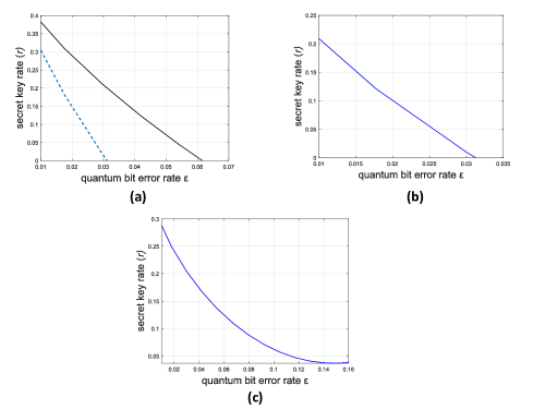
Figure 1: (Color online) Plot of the secret key rate as a function of quantum bit error rate $\mathcal{E}$: $(a)$ plot to evaluate a maximum tolerable error limit (security threshold) for sequence $S_{B1}$, solid (black) line and dashed (blue) line illustrate it for the situation with and without the introduction of the new variable $\mathcal{Y}$, respectively, $(b)$ plot to evaluate maximum tolerable error limit (security threshold) for sequence $S_{B2}$ without introducing new variable $\mathcal{X}$, and $(c)$ plot to evaluate maximum tolerable error limit (security threshold) for sequence $S_{B2}$ with the introduction of new variable $\mathcal{X}$.

We can now analyze the secret-key rate under the assumption that the protocol remains secure against collective attacks by Eve. Firstly, we will describe the initial state $\rho_{AB}^{n}$, and this description depends on the threshold QBER at which the protocol does not terminate prematurely. Thus, $\rho_{AB}^{n}$ represents a quantum state that should ideally be exclusively shared between Alice and Bob but is partially accessible to Eve, who can potentially perform collective attacks on it. Let’s define $\Gamma$ as the collection of all two-qubit states $\sigma_{AB}$ that can result from Eve’s collective attack on the initial state $\rho_{AB}^{n}$. The success of the attack is contingent on it leaving no discernible traces. In such a scenario, we must have $\sigma_{AB}^{\otimes n}=\rho_{AB}^{n}$. However, the attack may not always succeed; in cases where it fails, it leaves detectable traces, leading to the termination of the protocol. Our interest lies in situations where the protocol is not terminated. To account for the possibility of such a situation, we assume the existence of a protocol (operation) that Eve can utilize to produce a state $\sigma_{AB}^{\otimes n}=\rho_{AB}^{n}$ using ancillary qubits and a portion of the initial state shared by Alice and Bob, which is accessible to Eve through the channel. Following the approach in Ref. [31], we can define a set $\Gamma_{QBER}$ as a subset of $\Gamma$, containing all states $\sigma_{AB}$ for which the protocol does not terminate prematurely. In other words, if $\sigma_{AB}\in\Gamma_{QBER}$, then the protocol is expected to generate a secret key. Renner et al. in [31] have demonstrated that, based on the conditions outlined above, it is possible to establish both a lower bound and an upper bound on the secret-key rate for any protocol involving one-way post-processing.

$$r\geq\underset{c\leftarrow a}{sup}\underset{\sigma_{AB}\in\Gamma_{QBER}}{inf}\left(S(c|E)-H(c|b)\right).$$ (8)

here $r_{c\leftarrow a}$ is the rate that can be achieved if the channel $c\leftarrow a$ is used for the pre-processing, $S(c|E)$ denotes the von Neumann entropy of $c$ conditioned on Eve’s initial state i.e., $S(c|E)=S(\sigma_{cE})-S(\sigma_{E})$. This state $\sigma_{cE}$ is obtained from the two-qubit state $\sigma_{AB}$ by taking a purification $\sigma_{ABE}$ of the Bell diagonal state $\sigma_{AB}^{diag}:=\mathcal{O}_{2}(\sigma_{AB})$, state $\sigma_{AB}^{diag}$ has the same diagonal elements as in $\sigma_{AB}$ with respect to Bell basis. Here, $a$, $b$ and $e$ are the outcomes of Alice, Bob, and Eve’s after the measurement is applied to the first, second and third subsystem of $\sigma_{ABE}$.

To establish the upper limit for the rate, it suffices to focus exclusively on collective attacks. The composite system involving Alice, Bob, and Eve exhibits a product structure denoted as $\rho_{ABE}^{n}:=\sigma_{ABE}^{\otimes n}$, where $\sigma_{ABE}$ represents a tripartite state. The $n-$fold product state $\sigma_{abE}^{n}$ fully characterizes the scenario in which the single state $\sigma_{abE}$ is obtained when Alice and Bob perform measurements on the $\sigma_{ABE}$ state (for a detailed proof, please refer to Section IV of Ref.[31]). Consequently, the upper limit on the secret key rate is as follows:

$$r(a,b,e)=\underset{c\leftarrow a}{sup}\left(H(c|e)-H(c|b)\right).$$ (9)

This equation implies that if the supremum is taken over all the channels (including both quantum and classical channels) $c\leftarrow a$ will be the upper bound on the secret key rate.

Now, we analyze our protocol in the context of lower bound and upper bound of the secret key-rate. As before we take $n=1$, $\sigma_{AB}=\rho^{1}[\mu]$. It is required to consider a purification $|\Psi\rangle_{ABE}$ of the Bell diagonal state $\mathcal{O}_{2}(\sigma_{AB})$ originated from $\sigma_{AB}$ that can be written as,

$$|\Psi\rangle_{ABE}:=\stackrel{{\scriptstyle[}}{{i}}=1]{4}{\sum}\sqrt{\mu_{i}}|\varphi_{i}\rangle_{AB}\otimes|\varepsilon_{i}\rangle_{E},$$ (10)

where $|\varphi_{i}\rangle_{AB}$ denotes the Bell states which correspond to the joint system of Alice and Bob and $|\varepsilon_{i}\rangle_{E}$ denotes some mutually orthogonal states in Eve’s system which forms the basis $\varepsilon_{E}\in\left\{|\varepsilon_{1}\rangle_{E},\ldots,|\varepsilon_{4}\rangle_{E}\right\}$. It can be easily verified that Alice measures her qubit with $Z(X)$ basis and Bob measures his qubit with $Z$ or $X$ basis with equal probability, resulting in the outcomes of both parties $|\mathcal{A\rangle}$ and $|\mathcal{B\rangle},$ respectively. As an example, here we consider $|\mathcal{A\rangle}\in\left\{|0\rangle,|1\rangle\right\}$ and $|\mathcal{B\rangle}\in\left\{|0\rangle,|1\rangle,|+\rangle,|-\rangle\right\}$. Under this consideration, Eve’s state will be $|\phi^{\mathcal{A},\mathcal{B}}\rangle$, where

$$\begin{array}[]{lcl}|\phi^{0,0}\rangle&=&\frac{1}{\sqrt{2}}\left(\sqrt{\mu_{1}}|\varepsilon_{1}\rangle_{E}+\sqrt{\mu_{2}}|\varepsilon_{2}\rangle_{E}\right),\\ |\phi^{1,1}\rangle&=&\frac{1}{\sqrt{2}}\left(\sqrt{\mu_{1}}|\varepsilon_{1}\rangle_{E}-\sqrt{\mu_{2}}|\varepsilon_{2}\rangle_{E}\right),\\ |\phi^{0,1}\rangle&=&\frac{1}{\sqrt{2}}\left(\sqrt{\mu_{3}}|\varepsilon_{3}\rangle_{E}+\sqrt{\mu_{4}}|\varepsilon_{4}\rangle_{E}\right),\\ |\phi^{1,0}\rangle&=&\frac{1}{\sqrt{2}}\left(\sqrt{\mu_{3}}|\varepsilon_{3}\rangle_{E}-\sqrt{\mu_{4}}|\varepsilon_{4}\rangle_{E}\right),\\ |\phi^{0,+}\rangle&=&\frac{1}{2}\left(\sqrt{\mu_{1}}|\varepsilon_{1}\rangle_{E}+\sqrt{\mu_{2}}|\varepsilon_{2}\rangle_{E}+\sqrt{\mu_{3}}|\varepsilon_{3}\rangle_{E}+\sqrt{\mu_{4}}|\varepsilon_{4}\rangle_{E}\right),\\ |\phi^{0,-}\rangle&=&\frac{1}{2}\left(\sqrt{\mu_{1}}|\varepsilon_{1}\rangle_{E}+\sqrt{\mu_{2}}|\varepsilon_{2}\rangle_{E}-\sqrt{\mu_{3}}|\varepsilon_{3}\rangle_{E}-\sqrt{\mu_{4}}|\varepsilon_{4}\rangle_{E}\right),\\ |\phi^{1,+}\rangle&=&\frac{1}{2}\left(\sqrt{\mu_{1}}|\varepsilon_{1}\rangle_{E}-\sqrt{\mu_{2}}|\varepsilon_{2}\rangle_{E}+\sqrt{\mu_{3}}|\varepsilon_{3}\rangle_{E}-\sqrt{\mu_{4}}|\varepsilon_{4}\rangle_{E}\right),\\ |\phi^{1,-}\rangle&=&\frac{1}{2}\left(-\sqrt{\mu_{1}}|\varepsilon_{1}\rangle_{E}+\sqrt{\mu_{2}}|\varepsilon_{2}\rangle_{E}+\sqrt{\mu_{3}}|\varepsilon_{3}\rangle_{E}-\sqrt{\mu_{4}}|\varepsilon_{4}\rangle_{E}\right).\end{array}$$ (11)

We are now equipped to compute the density operators of Eve’s system for which Alice gets the outcome as $0$ and $1$, and denote them as $\sigma_{E}^{0}$ and $\sigma_{E}^{1},$ respectively. Here, we will consider the system that will be accepted by Alice and Bob after classical pre-processing of the protocol, which is given by $\sigma_{E}^{0}=\frac{1}{3}\left(P_{|\phi^{0,0}\rangle}+P_{|\phi^{0,1}\rangle}\right)+\frac{1}{6}\left(P_{|\phi^{0,+}\rangle}+P_{|\phi^{0,-}\rangle}\right)$ and $\sigma_{E}^{1}=\frac{1}{3}\left(P_{|\phi^{1,0}\rangle}+P_{|\phi^{1,1}\rangle}\right)+\frac{1}{6}\left(P_{|\phi^{1,+}\rangle}+P_{|\phi^{1,-}\rangle}\right)$ (for a more comprehensive calculation, refer to Appendix E). We can now obtain the state of Eve with respect to the basis $|\varepsilon_{i}\rangle_{E}$, where $i\in\{1,\cdots,4\}$ as

$$\sigma_{E}^{k}=\left(\begin{array}[]{cccc}\mu_{1}&(-1)^{k}\sqrt{\mu_{1}\mu_{2}}&0&0\\ (-1)^{k}\sqrt{\mu_{1}\mu_{2}}&\mu_{2}&0&0\\ 0&0&\mu_{3}&(-1)^{k}\sqrt{\mu_{1}\mu_{2}}\\ 0&0&(-1)^{k}\sqrt{\mu_{1}\mu_{2}}&\mu_{4}\end{array}\right),$$ (12)

where $k\in\left\{0,1\}\right\}.$

We have already mentioned channel $c\leftarrow a$ which provides a noisy version of $a$. We may consider that Alice uses bit-flip with probability $q$ to make $c$, i.e., $p_{c|a=0}(1)=p_{c|a=1}(0)=q$. We may now use the following standard relations to simplify the right hand side of Eq. (8)

$$\begin{array}[]{lcl}S(c|E)&=&S(cE)-S(E)\\ &=&\left[H(c)+S(E|c)-S(E)\right],\end{array}$$ (13)

and

$$\begin{array}[]{lcl}H(c|b)&=&H(cb)-H(b)\\ &=&\left[H(c)+H(b|c)-H(b)\right].\end{array}$$ (14)

Substituting Eq. (13) and Eq. (14) into the right hand side of Eq. (8), we can express the entropy difference as follows

$$S(c|E)-H(c|b)=S(E|c)-S(E)-\left(H(b|c)-H(b)\right).$$ (15)

The above substitution will modify Eq. (8) in a manner that will allow us to compute the lower bound of the secret key rate of our protocol.

If only Eve’s system is used for the calculation of the entropy, there would be only two possibilities, where Alice can have $0$ and $1$ bit value. At the same time, getting the entropy of $E$ conditioned on the value $c$, announced by Alice is dependent on bit flip probability. So we have,

$$S(E|c)=\frac{1}{2}S\left((1-q)\sigma_{E}^{0}+q\sigma_{E}^{1}\right)+\frac{1}{2}S\left(q\sigma_{E}^{0}+(1-q)\sigma_{E}^{1}\right),$$

and

$$S(E)=S\left(\frac{1}{2}\sigma_{E}^{0}+\frac{1}{2}\sigma_{E}^{1}\right).$$

Now, we consider Bob’s bit string, which he gets from the measurement result of his particle (system) $B$ in the state $|\Psi_{ABE}\rangle$. Intuitively, there must be two equal possibilities for getting the bit value $0$ and $1$ only when Bob’s bit string is considered. In addition, if the conditional entropy of Bob’s bit string is calculated provided by the noisy version of Alice’s bit ($c$ value) string, then error and no-error probability will also be considered. So we would have

$$H(b)=1$$

and

$$H(b|c)=h[q(1-\mathscr{\mathcal{E}})+(1-q)\mathcal{E}].$$

Using these expressions, for an optimal choice of the parameter $q$, we get the positive secret key if $\mathcal{E}\leq 0.124$ (see Fig. 2 (a)). We get this tolerable limit for error rate under the classical pre-processing i.e., noise introduced by Alice.

Let us now calculate the upper bound of the secret key rate using the Eq. (9). Here again, $|\phi^{0,0}\rangle$, $|\phi^{0,+}\rangle$, $|\phi^{1,1}\rangle$, and $|\phi^{1,-}\rangle$ are the states of Eve based on the event that Alice and Bob get the results $(0,0),(0,0),(1,1)$ and $(1,1),$ respectively. Inherently, we take the best situation for the adversary, Eve when she performs a von Neumann measurement with respect to the projectors along $\frac{1}{\sqrt{2}}(|\phi^{0,0}\rangle+|\phi^{1,1}\rangle),\frac{1}{\sqrt{2}}(|\phi^{0,0}\rangle-|\phi^{1,1}\rangle),\frac{1}{\sqrt{2}}(|\phi^{0,+}\rangle+|\phi^{0,+}\rangle),$ and $\frac{1}{\sqrt{2}}(|\phi^{0,+}\rangle-|\phi^{0,+}\rangle)$, to obtain an outcome $e$. Now, we can modify Eq. (9) by appropriately applying the above condition as follows,

$$\begin{array}[]{lcl}r(a,b,e)&=&H(c|e)-H(c|b)\\ &=&H(e|c)-H(e)-[H(b|c)-H(b)]\\ &\leq&\chi(E)-[H(b|c)-H(b)],\end{array}$$ (16)

here

$$\begin{array}[]{lcl}\chi(E)&=&S\left[\frac{1}{3}\left(P_{|\phi^{0,0}\rangle}+P_{|\phi^{1,1}\rangle}\right)+\frac{1}{6}\left(P_{|\phi^{0,+}\rangle}+P_{|\phi^{1,-}\rangle}\right)\right]\\ &-&\frac{1}{2}S\left[\left(1-q\right)\left(\frac{2}{3}P_{|\phi^{0,0}\rangle}+\frac{1}{3}P_{|\phi^{0,+}\rangle}\right)+q\left(\frac{2}{3}P_{|\phi^{1,1}\rangle}+\frac{1}{3}P_{|\phi^{1,-}\rangle}\right)\right]\\ &-&\frac{1}{2}S\left[q\left(\frac{2}{3}P_{|\phi^{0,0}\rangle}+\frac{1}{3}P_{|\phi^{0,+}\rangle}\right)+\left(1-q\right)\left(\frac{2}{3}P_{|\phi^{1,1}\rangle}+\frac{1}{3}P_{|\phi^{1,-}\rangle}\right)\right]\end{array}$$

is the Holevo quantity [33] that defines the maximum value of mutual information between $e$ and $c$ over all possible measurement scenarios that Eve can perform. This allows to compute the upper bound for the key rate by solving $r(a,b,e)=0$. The solution yields an upper bound as $\mathcal{E}\geq 0.114$ provided that optimal value of $q$ is used (cf. Fig. 2 (c)).

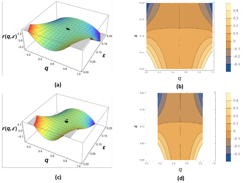
Figure 2: (Color online) Variation of secret key rate with bit-flip probability ($q$) and QBER ($\mathcal{E}$): $(a)$ lower bound on the secret-key rate of our protocol as function of bit-flip probability and QBER, $(b)$ contour plot for lower bound error limit; QBER vs bit-flip probability, $(c)$ upper bound on the secret-key rate of our protocol as function of bit-flip probability and QBER, and $(d)$ contour plot for upper bound error limit; QBER vs bit-flip probability.

IV Analysis of PNS attack

We have already mentioned that our schemes can be realized using WCP sources (see Eq. (1)). However, a cryptographic scheme based on WCP may face challenges due to the possibility of implementation of PNS and similar attacks by an eavesdropper. Thus, we need to establish the security of our schemes against different types of PNS attacks that can be implemented by an Eavesdropper (Eve) in a situation where $QBER=0$. The sub-protocols in our scheme require Bob to announce basis information or a set of non-orthogonal state information. Now, we may note the following.

1. In Protocol 1, Eve performs PNS attack with unlimited technological power within the regime of laws of physics. As the PNS attack in its original form requires quantum memory, it is also called quantum storage attack. Here, we consider the best scenario for Eve to attack. We want to mention that the probability of getting an $n$ photon state is $p(n,\mu)=\frac{e^{-\mu}\mu^{n}}{n!}$, here $\mu$ is the mean photon number. Alice and Bob know the channel transmittance ($\eta$) and $\mu$. Both parties would expect the probability of a non-zero photon without eavesdropping scenario to be $\underset{n\geq 1}{\sum}p(n,\mu\eta)$. Specifically, we consider a situation where Eve first counts the photon number with photon number quantum non-demolition measurement (QND), then she blocks the single-photon pulses and stores one photon from multi-photon pulses (from the sequence $S_{B1}$ and $S_{B2}$). It is further assumed that Eve subsequently sends the pulses to Alice with the remaining photons with lossless channel, $\eta=1$. As Eve performs PNS attack on the sequences $S_{B1}$ and $S_{B2}$, we have to consider the probability that Eve obtains multi-photon pulses in the same position of the two sequences. Here, we may consider the probability of attaining the above situation for Eve is $\left[\underset{n\geq 2}{\sum}p(n,\mu)\right]^{2}$. So, the information gained by Eve will be $I_{{\rm Eve1}}=\frac{0.625\times\left[\underset{n\geq 2}{\sum}p(n,\mu)\right]^{2}}{\underset{n\geq 1}{\sum}p(n,\mu\eta)}$, here we consider that the detectors are perfect. The factor $0.625$ arises due to the classical information revealed by Bob. We now draw a plot (see Fig. 3 (a)) to show the variation of $I_{{\rm Eve}1}$ with distance ($l$) for $\alpha=0.25$ dB/km and $\mu=0.1$. The estimated critical attenuation is $\delta_{c}=38.625$ dB and the corresponding critical distance in which the attacker knows all the bit information under the PNS attack is $l_{c}=154.5$ km. The critical length for the BB84 protocol under similar situation is 52 km [34] which is less than the critical length obtained for our protocol. Further, the graph shows that almost no information is revealed to Eve up to $70$ km. Beyond this point, the protocol becomes susceptible to a PNS attack up to a range of $150$ km. This advantage is achieved by employing more quantum signal or a greater number of quantum pieces.

2. In Protocol 2, the non-orthogonal state information is revealed by Bob. Here, Eve can implement a PNS-type attack which is usually referred to as the intercept resend with unambiguous discrimination (IRUD) attack. In this specific attack scenario, Eve initiates the process by conducting a photon number QND measurement and subsequently eliminates all the pulses containing less than three photons. Following this, she proceeds with the measurement $\mathcal{\mathscr{\mathcal{M}}}$. Eve prepares a new photon state after getting a conclusive result of the measurement $\mathcal{\mathscr{\mathcal{M}}}$ and sends that to Bob. Here we consider that Eve employs lossless channel and does not require quantum memory. Executing the protocol involves three rounds of transmitting qubit sequences between Alice and Bob. In order to carry out an IRUD attack, Eve would need to obtain conclusive results for the same positions in all three sequences, which isextremely improbable. To visualize it properly, the information gained by Eve through IRUD attack can be computed as $I_{{\rm Eve2}}=\frac{\left[I(3,\chi)p(3,\mu)\right]^{3}}{\underset{n\geq 1}{\sum}p(n,\mu\eta)},$ here $I(n,\chi)$ is the largest information that Eve can gain using $n$ photons present in one pulse, and $\chi$ is the overlap of two states within each set of non-orthogonal states which is announced by Bob. The power of the numerator of the expression $I_{{\rm Eve2}}$ is three as Eve need to get conclusive result consecutively for three rounds of transmission of the quantum sequences; and the probability $p(3,\mu)$ is used for Eve needs three proton state using lossless channel ($\eta=1$). Further, the denominator of the expression $I_{{\rm Eve2}}$ indicates the expected probability by Alice and Bob of non-zero photon state with known $\eta$. Here, we assume the value of $\alpha$ is $0.25$ dB/km and $\mu=0.2$; and illustrate the variation Eve’s information $(I_{Eve2})$ with distance to obtain the critical attenuation (see Fig. 3 (b)). From Fig. 3 (b), one can easily obtain critical attenuation $\delta_{c}=75.7$ dB and the corresponding distance $l_{c}=302.8$ km. Critical distance for SARG04 protocol under similar condition is 50 km [28] which is less than the critical length obtained for our Protocol. For this attack, almost no information is revealed to Eve up to $200$ km. It may be noted that this advantage over SARG04 protocol is obtained due to the increase in use of quantum pieces of information.

Figure 3: (Color online) Variation of Eve’s information with distance to obtain critical distance ($l_{c}$): $(a)$ Eve’s information as the function of distance to estimate the critical distance for which attacker get maximum key information by PNS attack on Protocol 1, $(b)$ Eve’s information as the function of distance to estimate the critical distance for which attacker gets maximum key information by IRUD attack on Protocol 2.

V Discussion

In this paper, we have proposed a new protocol for QKD and a variant of the same. The protocols consume more quantum resources compared to SARG04 or similar protocols, but transmit less classical information in public channel and thus reduces probability of some side channel attacks. Further, rigorous security analysis of the proposed protocols is performed. We have also calculated the tolerable error limit for the upper and lower bound of the secret key rate under a set of collective attacks. It is shown that by applying a certain type of classical pre-processing, the tolerable error limit can be increased and the same is illustrated through the graphs. Now, before we conclude, we may emphasize some of our important observations of our analysis. In the seminal paper [31], authors computed density operators of Eve’s final state for six-state QKD protocol. Interestingly, for our protocols, we have obtained the same expressions for the density operators describing the final system of Eve in spite of the fact that in our Protocol 2 (1) neither Alice nor Bob (Alice never) discloses the results of the measurements performed by them (her) in the cases where they have (she has) used different bases for preparation and measurement. The reason behind obtaining the same density operators for the system of Eve is that the terms that appear in the density matrix in the cases where basis mismatch happens cancel each other. Further, it is explicitly established that for the proposed protocols, the tolerable error limit of QBER $\mathcal{E}\leq 0.124$ for lower bound of key rate and $\mathcal{E}\geq 0.114$ for upper bound of key rate if classical pre-processing is used. In our case, the tolerable error limits are expected to decrease in absence of classical pre-processing.

In the practical implementation of cryptography, different kind of errors may happen during the transmission of qubits. Now if we consider $QBER>0$, then Eve can try to attack using partial cloning machines [36, 37, 38]. Acin et al., have shown that honest users of SARG04 can tolerate an error of up to 15% when Eve uses a best-known partial cloning machine. They further found that this value of tolerable error limit is greater than the corresponding tolerable error rate for the BB84 protocol. In our case for $QBER>0$ , the tolerable error limit is also computed to be 15% (cf. Section III) which is better than the BB84 protocol and its variants.

Security-efficiency trade-off for our protocol: In 2000, Cabello [29] introduced a measure of the efficiency of quantum communication protocols as $\eta=\frac{b_{s}}{q_{t}+b_{t}}$, where $b_{s}$ is the number of secret bits which can be exchanged by the protocol, $q_{t}$ is the number of qubits interchanged (by quantum channel) in each step of the protocol and $b_{t}$ is the classical bit information exchanged between Alice and Bob via classical channel. When we consider the sifting subprotocol of the second QKD protocol (Protocol 2), the values of the essential parameters are: $b_{s}=0.9375$, $q_{t}=3$, $b_{t}=0.75$ which gives the efficiency as $\eta=0.25$. When we consider the sifting subprotocol of our Protocol 1 for which, the values of the essential parameter are: $b_{s}=0.75$, $q_{t}=3$, $b_{t}=0.625$, and which gives the efficiency as $\eta=0.2069$ with no inherent error. For this specific sifting condition, the basis information will be revealed at end of the protocol which may increase the chance of PNS attack by the powerful Eve. To apply the Protocol 2 which is more efficient QKD protocol, one has to consider the inherent error probability value of $0.0625$, and the exchange of classical information is also more than the Protocol 1. We want to stress one point for the Protocol 2 that it is more robust against PNS attack as Alice and Bob have not revealed the basis information rather than two non-orthogonal state information is announced for the sifting process ($M$ value). Our two protocols are more efficient than the SARG04 protocol($\eta=0.125$.) and one can use one of our two protocols as per the requirement for the necessary task.

Acknowledgment:

Authors acknowledge support from the QUEST scheme of the Interdisciplinary Cyber-Physical Systems (ICPS) program of the Department of Science and Technology (DST), India, Grant No.: DST/ICPS/QuST/Theme-1/2019/14 (Q80). They also thank Kishore Thapliyal and Sandeep Mishra for their interest and useful technical feedback on this work.

Availability of data and materials

No additional data is needed for this work.

Competing interests

The authors declare that they have no competing interests.

Appendix A

It is already discussed in the main text that the Bell states are, $|\Phi^{\pm}\rangle\text{=$\frac{1}{\sqrt{2}}(|00\rangle\pm|11\rangle$)}$ and $|\Psi^{\pm}\rangle$$=\frac{1}{\sqrt{2}}(|01\rangle\pm|10\rangle)$. We can also express the Bell states in the diagonal basis as $|\Phi^{+}\rangle=\frac{1}{\sqrt{2}}\left(|++\rangle+|--\rangle\right)$, $|\Phi^{-}\rangle=\frac{1}{\sqrt{2}}\left(|+-\rangle+|-+\rangle\right)$, $|\Psi^{+}\rangle=\frac{1}{\sqrt{2}}\left(|++\rangle-|--\rangle\right)$, and $|\Psi^{-}\rangle=\frac{1}{\sqrt{2}}\left(|-+\rangle-|+-\rangle\right)$. We may now write from Eq. (3),

$$\begin{array}[]{lcl}\mu_{2}&=&\langle\Phi^{-}|\rho|\Phi^{-}\rangle\\ &=&\frac{1}{2}\left(\langle+-|\rho|+-\rangle+\langle+-|\rho|-+\rangle+\langle-+|\rho|+-\rangle+\langle-+|\rho|-+\rangle\right),\end{array}$$ (17)

$$\begin{array}[]{lcl}\mu_{4}&=&\langle\Psi^{-}|\rho|\Psi^{-}\rangle\\ &=&\frac{1}{2}\left(\langle+-|\rho|+-\rangle-\langle+-|\rho|-+\rangle-\langle-+|\rho|+-\rangle+\langle-+|\rho|-+\rangle\right),\end{array}$$ (18)

$$\begin{array}[]{lcl}\mu_{3}&=&\langle\Psi^{+}|\rho|\Psi^{+}\rangle\\ &=&\frac{1}{2}\left(\langle 01|\rho|01\rangle+\langle 01|\rho|10\rangle+\langle 10|\rho|01\rangle+\langle 10|\rho|10\rangle\right),\end{array}$$ (19)

and

$$\begin{array}[]{lcl}\mu_{4}&=&\langle\Psi^{+}|\rho|\Psi^{+}\rangle\\ &=&\frac{1}{2}\left(\langle 01|\rho|01\rangle-\langle 01|\rho|10\rangle-\langle 10|\rho|01\rangle+\langle 10|\rho|10\rangle\right).\end{array}$$ (20)

We consider $\mathcal{E}$ to be a symmetric error, and therefore, the following relationships are to be valid,

$$\begin{array}[]{lcl}\langle 00|\rho|00\rangle+\langle 11|\rho|11\rangle&=&1-\mathcal{E},\\ \langle++|\rho|++\rangle+\langle--|\rho|--\rangle&=&1-\mathcal{E},\\ \langle 01|\rho|01\rangle+\langle 10|\rho|10\rangle&=&\mathcal{E},\\ \langle+-|\rho|+-\rangle+\langle-+|\rho|-+\rangle&=&\mathcal{E}.\end{array}$$ (21)

Inserting these Eqs. (17), (18), (19), and (20) in the relation (21), we obtain

$$\begin{array}[]{lcl}\mu_{2}+\mu_{4}&=&\left(\langle+-|\rho|+-\rangle+\langle-+|\rho|-+\rangle\right)=\mathcal{E}\\ \mu_{2}&=&\mathcal{E}-\mu_{4}\end{array},$$

and

$$\begin{array}[]{lcl}\mu_{3}+\mu_{4}&=&\left(\langle 01|\rho|01\rangle+\langle 10|\rho|10\rangle\right)=\mathcal{E}\\ \mu_{3}&=&\mathcal{E}-\mu_{4}.\end{array}.$$

Now, total probability must satisfy $\mu_{1}+\mu_{2}+\mu_{3}+\mu_{4}=1$. By employing the aforementioned connection with the preceding outcomes, we obtain, $\mu_{1}=1-2\mathcal{E}+\mu_{4}$ and $\mu_{2}=\mu_{3}=\mathcal{E}-\mu_{4}$.

Appendix B

We use these relations to compute the key rate. The conditional probability, $Pr\left(B=|i\rangle\left|A=|j\rangle\right.\right)=\frac{Pr(B=|i\rangle,A=|j\rangle)}{Pr(A=|j\rangle)}$ and conditional entropy,

$$H(B|A)=-\sum_{j}Pr(A=|j\rangle)\sum_{i}Pr(B=|i\rangle|A=|j\rangle)\log_{2}Pr(B=|i\rangle|A=|j\rangle),$$ (22)

$$\begin{array}[]{lcl}Pr\left(B=|0\rangle|A=|0\rangle\right)=Pr\left(B=|1\rangle|A=|1\rangle\right)&=&\frac{\mu_{1}+\mu_{2}}{2},\\ Pr\left(B=|1\rangle|A=|0\rangle\right)=Pr\left(B=|0\rangle|A=|1\rangle\right)&=&\frac{\mu_{3}+\mu_{4}}{2},\\ Pr\left(B=|+\rangle|A=|+\rangle\right)=Pr\left(B=|-\rangle|A=|-\rangle\right)&=&\frac{\mu_{1}+\mu_{3}}{2},\\ Pr\left(B=|-\rangle|A=|+\rangle\right)=Pr\left(B=|+\rangle|A=|-\rangle\right)&=&\frac{\mu_{2}+\mu_{4}}{2},\end{array}$$

$$Pr\left(B=|i\rangle|A=|j\rangle\right)=\frac{1}{4},$$

$$Pr\left(B=|i\rangle\right)=\frac{1}{4},$$

here $i\neq j$ and $i,j\in\{|0\rangle,|1\rangle,|+\rangle,|-\rangle,\}$. Now, using Eq. (22) we can obtain

$$\begin{array}[]{lcl}H(B|A)&=&-\frac{\mu_{1}+\mu_{2}}{4}\log_{2}\frac{\mu_{1}+\mu_{2}}{2}-\frac{\mu_{3}+\mu_{4}}{4}\log_{2}\frac{\mu_{3}+\mu_{4}}{2}\\ &-&\frac{\mu_{1}+\mu_{3}}{4}\log_{2}\frac{\mu_{1}+\mu_{3}}{2}-\frac{\mu_{2}+\mu_{4}}{4}\log_{2}\frac{\mu_{2}+\mu_{4}}{2}-\frac{1}{2}\log_{2}\frac{1}{4}\\ &=&-\frac{1-\mathcal{E}}{2}\log_{2}\frac{1-\mathcal{E}}{2}-\frac{\mathcal{E}}{2}\log_{2}\frac{\mathcal{E}}{2}+1,\end{array}$$

and

$$\begin{array}[]{lcl}H(B)&=&-4\times\frac{1}{4}\log_{2}\frac{1}{4}\\ &=&2\end{array}.$$

Therefore,

$$\begin{array}[]{lcl}I(A:B)&=&H(B)-H(B|A)\\ &=&1+\frac{1-\mathcal{E}}{2}\log_{2}\frac{1-\mathcal{E}}{2}+\frac{\mathcal{E}}{2}\log_{2}\frac{\mathcal{E}}{2},\end{array}$$

using the secret key rate we have,

$$\begin{array}[]{lcl}r&=&I(A:B)-H(V)\\ &=&1+\frac{1-\mathcal{E}}{2}\log_{2}\frac{1-\mathcal{E}}{2}+\frac{\mathcal{E}}{2}\log_{2}\frac{\mathcal{E}}{2}-2h(\mathcal{E}).\end{array}$$

Appendix C

Here, we calculate the key rate equation after the key-sifting subprotocol by the both parties which means that the probability in acceptable condition will be considered.

$$\begin{array}[]{lcl}Pr\left(b=0|a=0\right)=Pr\left(b=1|a=1\right)&=&\frac{1}{6}+\frac{2\mu_{1}+\mu_{2}+\mu_{3}}{3},\\ Pr\left(b=0|a=1\right)=Pr\left(b=1|a=0\right)&=&\frac{1}{6}+\frac{\mu_{2}+\mu_{3}+2\mu_{4}}{3},\end{array}$$

$$\begin{array}[]{lcl}Pr\left(b=0\right)=Pr\left(b=1\right)&=&\frac{1}{2},\end{array}$$

in the similar approach for Eq. (22) we have,

$$\begin{array}[]{lcl}H(b|a)&=&-\frac{1+4\mu_{1}+2\mu_{2}+2\mu_{3}}{6}\log_{2}\frac{1+4\mu_{1}+2\mu_{2}+2\mu_{3}}{6}-\frac{1+2\mu_{2}+2\mu_{3}+4\mu_{4}}{6}\log_{2}\frac{1+2\mu_{2}+2\mu_{3}+4\mu_{4}}{6}\\ &=&-\frac{5-4\mathcal{E}}{6}\log_{2}\frac{5-4\mathcal{E}}{6}-\frac{1+4\mathcal{E}}{6}\log_{2}\frac{1+4\mathcal{E}}{6}\\ &=&h\left(\frac{1}{6}+\frac{2\mathcal{E}}{3}\right),\end{array}$$

$$\begin{array}[]{lcl}I(a|b)&=&H(b)-H(b|a)\\ &=&-\frac{1}{2}\log_{2}\frac{1}{2}-h(b|a)\\ &=&1-h\left(\frac{1}{6}+\frac{2\mathcal{E}}{3}\right),\end{array}$$

so the final expression for secret key rate,

$$\begin{array}[]{lcl}r&=&I(a|b)-H(V)\\ &=&1-h\left(\frac{1}{6}+\frac{2\mathcal{E}}{3}\right)-2h(\mathcal{E}).\end{array}$$

Appendix D

Alice and Bob are evaluating the security threshold of the particle sequences, denoted as $S_{A}$ and $S_{B1}$, when they employ the same basis for preparing or measuring the states. We can define the absence of errors (or the presence of errors) when they measure the states $|\Phi^{\pm}\rangle(|\Psi^{\pm}\rangle)$ using the computational basis. Similarly, there will be an absence of errors (or the presence of errors) when both Alice and Bob measure the states $|\Phi^{+}\rangle$ and $|\Psi^{+}\rangle$ (or $|\Phi^{-}\rangle$ and $|\Psi^{-}\rangle$) with the diagonal basis. These scenarios lead to a total of four cases that we need to consider. Furthermore, we can conclude that the state $\rho$ can be measured with equal probability by both Alice and Bob using both the computational and diagonal bases. We will begin with an illustrative example to enhance comprehension. Let us consider the scenario where two parties measure the Bell states $|\Phi^{+}\rangle$ and $|\Psi^{+}\rangle$ in the computational basis. The resulting probabilities of encountering no error and error are $\frac{\mu_{1}}{2}$ and $\frac{\mu_{3}}{2}$, respectively. Consequently, the probabilities of experiencing no error and error when measuring the states $|\Phi^{+}\rangle$ and $|\Psi^{+}\rangle$ are $\frac{1-\mathcal{E}}{2}$ and $\frac{\mathcal{E}}{2}$, respectively. It is evident that the probability of encountering no error and error when measuring the states $|\Phi^{+}\rangle$ and $|\Psi^{+}\rangle$ in the computational basis, considering the total number of qubits, can be expressed as $\frac{\frac{\mu_{1}}{2}}{\frac{1-\mathcal{E}}{2}}$ and $\frac{\frac{\mu_{3}}{2}}{\frac{\mathcal{E}}{2}}$, which simplifies to$\frac{\mu_{1}}{1-\mathcal{E}}$ and $\frac{\mu_{3}}{\mathcal{E}}$, respectively. Similarly, when measuring the states $|\Phi^{-}\rangle$ and $|\Psi^{-}\rangle$ in the computational basis, the probabilities of encountering no error and error can be expressed as $\frac{\mu_{2}}{1-\mathcal{E}}$ and $\frac{\mu_{4}}{\mathcal{E}}$. Moving on to the diagonal basis, the probabilities of encountering no error and error when measuring the states $|\Phi^{+}\rangle$ and $|\Psi^{+}\rangle$ are $\frac{\mu_{1}}{1-\mathcal{E}}$ and $\frac{\mu_{3}}{1-\mathcal{E}}$, respectively. Similarly, for the states $|\Phi^{-}\rangle$ and |$\Psi^{-}\rangle$, the probabilities are $\frac{\mu_{2}}{\mathcal{E}}$ and $\frac{\mu_{4}}{\mathcal{E}}$. In a scenario where no errors occur, one can calculate the entropy as follows:

$$\begin{array}[]{lcl}{\rm H}_{{\rm no-error}}&=&-\frac{1}{2}\left[\frac{\mu_{1}}{1-\mathcal{E}}\log_{2}\frac{\mu_{1}}{1-\mathcal{E}}+\frac{\mu_{2}}{1-\mathcal{E}}\log_{2}\frac{\mu_{2}}{1-\mathcal{E}}+\frac{\mu_{1}}{1-\mathcal{E}}\log_{2}\frac{\mu_{1}}{1-\mathcal{E}}+\frac{\mu_{3}}{1-\mathcal{E}}\log_{2}\frac{\mu_{3}}{1-\mathcal{E}}\right]\\ &=&-\frac{1}{2}\left[\frac{2\mu_{1}}{1-\mathcal{E}}\log_{2}\frac{\mu_{1}}{1-\mathcal{E}}+\frac{2\mu_{2}}{1-\mathcal{E}}\log_{2}\frac{\mu_{2}}{1-\mathcal{E}}\right]\,\,\,\,{\rm as}\,\,\mu_{2}=\mu_{3}\\ &=&-\left[\frac{\left(1-2\mathcal{E}+\mu_{4}\right)}{1-\mathcal{E}}\log_{2}\frac{\left(1-2\mathcal{E}+\mu_{4}\right)}{1-\mathcal{E}}+\frac{\left(\mathcal{E}-\mu_{4}\right)}{1-\mathcal{E}}\log_{2}\frac{\left(\mathcal{E}-\mu_{4}\right)}{1-\mathcal{E}}\right]\,\,\,\,({\rm using\,the\,results\,of\,Appendix\,A})\\ &=&h\left(\frac{1-2\mathcal{E}+\mu_{4}}{1-\mathcal{E}}\right),\end{array}$$

and in presence of error the entropy can be computed as,

$$\begin{array}[]{lcl}{\rm H_{error}}&=&-\frac{1}{2}\left[\frac{\mu_{3}}{\mathcal{E}}\log_{2}\frac{\mu_{3}}{\mathcal{E}}+\frac{\mu_{4}}{\mathcal{E}}\log_{2}\frac{\mu_{4}}{\mathcal{E}}+\frac{\mu_{2}}{\mathcal{E}}\log_{2}\frac{\mu_{2}}{\mathcal{E}}+\frac{\mu_{4}}{\mathcal{E}}\log_{2}\frac{\mu_{4}}{\mathcal{E}}\right]\\ &=&-\frac{1}{2}\left[\frac{2\mu_{2}}{\mathcal{E}}\log_{2}\frac{2\mu_{2}}{\mathcal{E}}+\frac{2\mu_{4}}{\mathcal{E}}\log_{2}\frac{2\mu_{4}}{\mathcal{E}}\right]\,\,{\rm as}\,\mu_{2}=\mu_{3}\\ &=&-\left[\frac{\left(\mathcal{E}-\mu_{4}\right)}{\mathcal{E}}\log_{2}\frac{\left(\mathcal{E}-\mu_{4}\right)}{\mathcal{E}}+\frac{\mu_{4}}{\mathcal{E}}\log_{2}\frac{\mu_{4}}{\mathcal{E}}\right]\,\,({\rm using\,the\,results\,of\,Appendix\,A})\\ &=&h\left(\frac{\mathcal{E}-\mu_{4}}{\mathcal{E}}\right).\end{array}$$

After conducting statistical averaging for both no error and error scenarios, we acquire,

$$\begin{array}[]{l}\left(1-\mathcal{E}\right){\rm H}_{{\rm no-error}}+\mathcal{E}H_{error}\\ =\left(1-\mathcal{E}\right)h\left(\frac{1-2\mathcal{E}+\mu_{4}}{1-\mathcal{E}}\right)+\mathcal{E}h\left(\frac{\mathcal{E}-\mu_{4}}{\mathcal{E}}\right)\\ =-\left(1-\mathcal{E}\right)\left[\frac{\left(1-2\mathcal{E}+\mu_{4}\right)}{1-\mathcal{E}}\log_{2}\frac{\left(1-2\mathcal{E}+\mu_{4}\right)}{1-\mathcal{E}}+\frac{\left(\mathcal{E}-\mu_{4}\right)}{1-\mathcal{E}}\log_{2}\frac{\left(\mathcal{E}-\mu_{4}\right)}{1-\mathcal{E}}\right]\\ -\mathcal{E}\left[\frac{\left(\mathcal{E}-\mu_{4}\right)}{\mathcal{E}}\log_{2}\frac{\left(\mathcal{E}-\mu_{4}\right)}{\mathcal{E}}+\frac{\mu_{4}}{\mathcal{E}}\log_{2}\frac{\mu_{4}}{\mathcal{E}}\right]\\ =-\left[\left(1-2\mathcal{E}+\mu_{4}\right)\log_{2}\left(1-2\mathcal{E}+\mu_{4}\right)+\left(\mathcal{E}-\mu_{4}\right)\log_{2}\left(\mathcal{E}-\mu_{4}\right)-\left(1-2\mathcal{E}+\mu_{4}\right)\log_{2}\left(1-\mathcal{E}\right)-\left(\mathcal{E}-\mu_{4}\right)\log_{2}\left(1-\mathcal{E}\right)\right]\\ -\left[\left(\mathcal{E}-\mu_{4}\right)\log_{2}\left(\mathcal{E}-\mu_{4}\right)+\mu_{4}\log_{2}\mu_{4}-\left(\mathcal{E}-\mu_{4}\right)\log_{2}\mathcal{E}-\mu_{4}\log_{2}\mathcal{E}\right]\\ =-\left[\left(1-2\mathcal{E}+\mu_{4}\right)\log_{2}\left(1-2\mathcal{E}+\mu_{4}\right)+2\left(\mathcal{E}-\mu_{4}\right)\log_{2}\left(\mathcal{E}-\mu_{4}\right)+\mu_{4}\log_{2}\mu_{4}\right]\\ +\left(1-2\mathcal{E}+\mu_{4}+\mathcal{E}-\mu_{4}\right)\log_{2}\left(1-\mathcal{E}\right)+\left(\mathcal{E}-\mu_{4}+\mu_{4}\right)\log_{2}\mathcal{E}\\ =H(V)+\left(1-\mathcal{E}\right)\log_{2}\left(1-\mathcal{E}\right)+\mathcal{E}\log_{2}\mathcal{E}\\ =H(V)-h(\mathcal{E}).\end{array}$$

Appendix E

In this appendix, we provide a detailed of the mathematical processes involved in obtaining Eq. (12) from Eq. (10) in Section III. To begin with, let us focus on a scenario in which both Alice and Bob perform measurements on their qubits using the $Z$ basis (similar outcomes are observed for the $X$ basis as well).

$$\begin{array}[]{lcl}|\Psi\rangle_{ABE}&:=&\stackrel{{\scriptstyle[}}{{i}}=1]{4}{\sum}\sqrt{\mu_{i}}|\varphi_{i}\rangle_{AB}\otimes|\varepsilon_{i}\rangle_{E}\\ &=&\frac{1}{2\sqrt{2}}\left[\sqrt{\mu_{1}}\left(|00\rangle+|11\rangle\right)\otimes|\varepsilon_{1}\rangle+\sqrt{\mu_{2}}\left(|00\rangle-|11\rangle\right)\otimes|\varepsilon_{2}\rangle\right.\\ &+&\left.\sqrt{\mu_{3}}\left(|01\rangle+|10\rangle\right)\otimes|\varepsilon_{3}\rangle+\sqrt{\mu_{4}}\left(|01\rangle-|10\rangle\right)\otimes|\varepsilon_{4}\rangle\right]_{ABE}\\ &=&\frac{1}{2\sqrt{2}}\left[|00\rangle\left(\sqrt{\mu_{1}}|\varepsilon_{1}\rangle+\sqrt{\mu_{2}}|\varepsilon_{2}\rangle\right)+|11\rangle\left(\sqrt{\mu_{1}}|\varepsilon_{1}\rangle-\sqrt{\mu_{2}}|\varepsilon_{2}\rangle\right)\right.\\ &+&\left.|01\rangle\left(\sqrt{\mu_{3}}|\varepsilon_{3}\rangle+\sqrt{\mu_{4}}|\varepsilon_{4}\rangle\right)+|10\rangle\left(\sqrt{\mu_{3}}|\varepsilon_{3}\rangle-\sqrt{\mu_{4}}|\varepsilon_{4}\rangle\right)\right]_{ABE}\\ &=&\frac{1}{2}\left[|00\rangle\otimes|\phi^{0,0}\rangle+|11\rangle\otimes|\phi^{1,1}\rangle+|01\rangle\otimes|\phi^{0,1}\rangle+|10\rangle\otimes\rangle\right]_{ABE}\end{array}.$$

Now, let’s consider the scenario in which Alice and Bob measure their qubits using the $Z$ and $X$ bases, respectively,

$$\begin{array}[]{lcl}|\Psi\rangle_{ABE}&:=&\stackrel{{\scriptstyle[}}{{i}}=1]{4}{\sum}\sqrt{\mu_{i}}|\varphi_{i}\rangle_{AB}\otimes|\varepsilon_{i}\rangle_{E}\\ &=&\frac{1}{2\sqrt{2}}\left[\sqrt{\mu_{1}}\left(|00\rangle+|11\rangle\right)\otimes|\varepsilon_{1}\rangle+\sqrt{\mu_{2}}\left(|00\rangle-|11\rangle\right)\otimes|\varepsilon_{2}\rangle\right.\\ &+&\left.\sqrt{\mu_{3}}\left(|01\rangle+|10\rangle\right)\otimes|\varepsilon_{3}\rangle+\sqrt{\mu_{4}}\left(|01\rangle-|10\rangle\right)\otimes|\varepsilon_{4}\rangle\right]_{ABE}\\ &=&\frac{1}{4}\left[\sqrt{\mu_{1}}\left\{|0\rangle\left(|+\rangle+|-\rangle\right)+|1\rangle\left(|+\rangle-|-\rangle\right)\right\}|\varepsilon_{1}\rangle\right.\\ &+&\sqrt{\mu_{2}}\left\{|0\rangle\left(|+\rangle+|-\rangle\right)-|1\rangle\left(|+\rangle-|-\rangle\right)\right\}|\varepsilon_{2}\rangle\\ &+&\sqrt{\mu_{3}}\left\{|0\rangle\left(|+\rangle-|-\rangle\right)+|1\rangle\left(|+\rangle+|-\rangle\right)\right\}|\varepsilon_{3}\rangle\\ &+&\left.\sqrt{\mu_{4}}\left\{|0\rangle\left(|+\rangle-|-\rangle\right)-|1\rangle\left(|+\rangle+|-\rangle\right)\right\}|\varepsilon_{4}\rangle\right]_{ABE}\\ &=&\frac{1}{4}\left[|0+\rangle\left\{\sqrt{\mu_{1}}|\varepsilon_{1}\rangle+\sqrt{\mu_{2}}|\varepsilon_{2}\rangle+\sqrt{\mu_{3}}|\varepsilon_{3}\rangle+\sqrt{\mu_{4}}|\varepsilon_{4}\rangle\right\}\right.\\ &+&|0-\rangle\left\{\sqrt{\mu_{1}}|\varepsilon_{1}\rangle+\sqrt{\mu_{2}}|\varepsilon_{2}\rangle-\sqrt{\mu_{3}}|\varepsilon_{3}\rangle-\sqrt{\mu_{4}}|\varepsilon_{4}\rangle\right\}\\ &+&|1+\rangle\left\{\sqrt{\mu_{1}}|\varepsilon_{1}\rangle-\sqrt{\mu_{2}}|\varepsilon_{2}\rangle+\sqrt{\mu_{3}}|\varepsilon_{3}\rangle-\sqrt{\mu_{4}}|\varepsilon_{4}\rangle\right\}\\ &+&\left.|1-\rangle\left\{-\sqrt{\mu_{1}}|\varepsilon_{1}\rangle+\sqrt{\mu_{2}}|\varepsilon_{2}\rangle+\sqrt{\mu_{3}}|\varepsilon_{3}\rangle-\sqrt{\mu_{4}}|\varepsilon_{4}\rangle\right\}\right]_{ABE}\\ &=&\frac{1}{2}\left[|0+\rangle|\phi^{0,+}\rangle+|0-\rangle|\phi^{0,-}\rangle+|1+\rangle|\phi^{1,+}\rangle+|1-\rangle|\phi^{1,-}\rangle\right]_{ABE}\end{array},$$

In the main text, we have provided the details of Eve’s initial state denoted as $\varepsilon_{E}$, as well as Eve’s state $|\phi^{\mathcal{A},\mathcal{B}}\rangle$ after Alice and Bob’s measurement. Our focus is solely on the instances that Alice and Bob accept after the classical pre-processing stage. Following normalization, we examine the density operator of Eve’s system specifically when Alice obtains the outcome $0$,

$$\begin{array}[]{lcl}\sigma_{E}^{0}&=&\frac{1}{3}\left[|\phi^{0,0}\rangle\langle\phi^{0,0}|+|\phi^{0,1}\rangle\langle\phi^{0,1}|\right]+\frac{1}{6}\left[|\phi^{0,+}\rangle\langle\phi^{0,+}|+|\phi^{0,-}\rangle\langle\phi^{0,-}|\right]\\ &=&\frac{1}{3}\left(P_{|\phi^{0,0}\rangle}+P_{|\phi^{0,1}\rangle}\right)+\frac{1}{6}\left(P_{|\phi^{0,+}\rangle}+P_{|\phi^{0,-}\rangle}\right)\end{array},$$

and when Alice obtains the outcome $1$ is,

$$\begin{array}[]{lcl}\sigma_{E}^{1}&=&\frac{1}{3}\left[|\phi^{1,0}\rangle\langle\phi^{1,0}|+|\phi^{1,1}\rangle\langle\phi^{1,1}|\right]+\frac{1}{6}\left[|\phi^{1,+}\rangle\langle\phi^{1,+}|+|\phi^{1,-}\rangle\langle\phi^{1,-}|\right]\\ &=&\frac{1}{3}\left(P_{|\phi^{1,0}\rangle}+P_{|\phi^{1,1}\rangle}\right)+\frac{1}{6}\left(P_{|\phi^{1,+}\rangle}+P_{|\phi^{1,-}\rangle}\right)\end{array}.$$

References

- [1] Ronald L Rivest, Adi Shamir, and Leonard Adleman. A method for obtaining digital signatures and public-key cryptosystems. Communications of the ACM, 21(2):120–126, 1978.
- [2] Whitfield Diffie and Martin Hellman. New directions in cryptography. IEEE Transactions on Information Theory, 22(6):644–654, 1976.
- [3] Anirban Pathak. Elements of quantum computation and quantum communication. CRC Press Boca Raton, 2013.
- [4] Peter W Shor. Algorithms for quantum computation: discrete logarithms and factoring. In Proceedings 35th Annual Symposium on Foundations of Computer Science, pages 124–134. IEEE, 1994.
- [5] Charles H. Bennett and Gilles Brassard. Quantum cryptography: Public-key distribution and coin tossing, in Proc. IEEE Int. Conf. on Computers, Systems, and Signal Processing (Bangalore, India, 1984), pp. 175-179., 1984.
- [6] William K Wootters and Wojciech H Zurek. A single quantum cannot be cloned. Nature, 299(5886):802–803, 1982.
- [7] Charles H Bennett. Quantum cryptography using any two nonorthogonal states. Physical Review Letters, 68(21):3121, 1992.
- [8] Artur K Ekert. Quantum cryptography based on Bell’s theorem. Physical Review Letters, 67(6):661, 1991.
- [9] Lior Goldenberg and Lev Vaidman. Quantum cryptography based on orthogonal states. Physical Review Letters, 75(7):1239, 1995.
- [10] S Srikara, Kishore Thapliyal, and Anirban Pathak. Continuous variable direct secure quantum communication using gaussian states. Quantum Information Processing, 19(4):132, 2020.
- [11] Preeti Yadav, R Srikanth, and Anirban Pathak. Two-step orthogonal-state-based protocol of quantum secure direct communication with the help of order-rearrangement technique. Quantum Information Processing, 13(12):2731–2743, 2014.
- [12] Chitra Shukla, Vivek Kothari, Anindita Banerjee, and Anirban Pathak. On the group-theoretic structure of a class of quantum dialogue protocols. Physics Letters A, 377(7):518–527, 2013.
- [13] Lin Liu, Min Xiao, and Xiuli Song. Authenticated semiquantum dialogue with secure delegated quantum computation over a collective noise channel. Quantum Information Processing, 17(12):342, 2018.
- [14] Anindita Banerjee, Chitra Shukla, Kishore Thapliyal, Anirban Pathak, and Prasanta K Panigrahi. Asymmetric quantum dialogue in noisy environment. Quantum Information Processing, 16(2):49, 2017.
- [15] Chitra Shukla, Kishore Thapliyal, and Anirban Pathak. Semi-quantum communication: protocols for key agreement, controlled secure direct communication and dialogue. Quantum Information Processing, 16(12):295, 2017.
- [16] Kishore Thapliyal, Rishi Dutt Sharma, and Anirban Pathak. Orthogonal-state-based and semi-quantum protocols for quantum private comparison in noisy environment. International Journal of Quantum Information, 16(05):1850047, 2018.
- [17] Kishore Thapliyal and Anirban Pathak. Applications of quantum cryptographic switch: various tasks related to controlled quantum communication can be performed using Bell states and permutation of particles. Quantum Information Processing, 14(7):2599–2616, 2015.
- [18] Arindam Dutta and Anirban Pathak. Collective attack free controlled quantum key agreement without quantum memory. arXiv preprint arXiv:2308.05470, 2023.
- [19] Akshata Shenoy-Hejamadi, Anirban Pathak, and Srikanth Radhakrishna. Quantum cryptography: key distribution and beyond. Quanta, 6(1):1–47, 2017.
- [20] Nicolas Gisin, Grégoire Ribordy, Wolfgang Tittel, and Hugo Zbinden. Quantum cryptography. Reviews of Modern Physics, 74(1):145, 2002.
- [21] Marcos Curty and David J Santos. Quantum authentication of classical messages. Physical Review A, 64(6):062309, 2001.
- [22] Arindam Dutta and Anirban Pathak. A short review on quantum identity authentication protocols: How would Bob know that he is talking with Alice? Quantum Information Processing, 21:369, 2022.
- [23] Arindam Dutta and Anirban Pathak. Controlled secure direct quantum communication inspired scheme for quantum identity authentication. Quantum Information Processing, 22:13, 2022.
- [24] Chao-Yang Lu and Jian-Wei Pan. Quantum-dot single-photon sources for the quantum internet. Nature Nanotechnology, 16(12):1294–1296, 2021.
- [25] Sarah Thomas and Pascale Senellart. The race for the ideal single-photon source is on. Nature Nanotechnology, 16(4):367–368, 2021.
- [26] Bruno Huttner, Nobuyuki Imoto, Nicolas Gisin, and Tsafrir Mor. Quantum cryptography with coherent states. Physical Review A, 51(3):1863, 1995.
- [27] Gilles Brassard, Norbert Lütkenhaus, Tal Mor, and Barry C Sanders. Limitations on practical quantum cryptography. Physical Review Letters, 85(6):1330, 2000.
- [28] Valerio Scarani, Antonio Acin, Grégoire Ribordy, and Nicolas Gisin. Quantum cryptography protocols robust against photon number splitting attacks for weak laser pulse implementations. Physical Review Letters, 92(5):057901, 2004.
- [29] Adán Cabello. Quantum key distribution in the holevo limit. Physical Review Letters, 85(26):5635, 2000.
- [30] Barbara Kraus, Nicolas Gisin, and Renato Renner. Lower and upper bounds on the secret-key rate for quantum key distribution protocols using one-way classical communication. Physical Review Letters, 95(8):080501, 2005.
- [31] Renato Renner, Nicolas Gisin, and Barbara Kraus. Information-theoretic security proof for quantum-key-distribution protocols. Physical Review A, 72(1):012332, 2005.
- [32] Matthias Christandl, Renato Renner, and Artur Ekert. A generic security proof for quantum key distribution. arXiv preprint quant-ph/0402131, 2004.
- [33] Alexander Semenovich Holevo. Bounds for the quantity of information transmitted by a quantum communication channel. Problemy Peredachi Informatsii, 9(3):3–11, 1973.
- [34] Antonio Acin, Nicolas Gisin, and Valerio Scarani. Coherent-pulse implementations of quantum cryptography protocols resistant to photon-number-splitting attacks. Physical Review A, 69(1):012309, 2004.
- [35] Asher Peres. Quantum theory: concepts and methods. Springer, 1997.
- [36] Nicolas J Cerf and Sofyan Iblisdir. Optimal n-to-m cloning of conjugate quantum variables. Physical Review A, 62(4):040301, 2000.
- [37] Chi-Sheng Niu and Robert B Griffiths. Optimal copying of one quantum bit. Physical Review A, 58(6):4377, 1998.
- [38] Nicolas J Cerf. Pauli cloning of a quantum bit. Physical Review Letters, 84(19):4497, 2000.