Measurement of the absolute branching fraction of the inclusive decay $D^{+}_{s}\rightarrow\pi^{+}\pi^{+}\pi^{-}X$

Abstract

Using an $e^{+}e^{-}$ collision data sample with a total integrated luminosity of $3.19$ fb^-1 collected with the BESIII detector at a center-of-mass energy of 4.178 GeV, the branching fraction of the inclusive decay of the $D^{+}_{s}$ meson to final states including at least three charged pions is measured for the first time to be ${\cal B}(D^{+}_{s}\rightarrow\pi^{+}\pi^{+}\pi^{-}X)=(32.81\pm 0.35_{\rm stat}\pm{0.63_{\rm syst}})\%$. In this measurement the charged pions from $K^{0}_{\scriptscriptstyle S}$ meson decays are excluded. The partial branching fractions of $D^{+}_{s}\rightarrow\pi^{+}\pi^{+}\pi^{-}X$ are also measured as a function of the $\pi^{+}\pi^{+}\pi^{-}$ invariant mass.

I Introduction

Lepton flavor universality (LFU) is a very hot topic in the field of particle physics. Recent reports from several high energy experiments studying $B$ meson semileptonic decays of the form $B\rightarrow D^{(*)}{\ell}^{+}\nu_{\ell}$ ($\ell=e$, $\mu$, or $\tau$) suggest tensions with Standard Model based predictions hflav , and have drawn attention from both experimentalists and theorists. Among these results, the LHCb measurement of the ratio of the branching fractions (BFs) of the $B^{0}$ meson semileptonic decays, ${\cal R}(D^{*-})\equiv{\cal B}(B^{0}\rightarrow D^{*-}\tau^{+}\nu_{\tau})/{\cal B}(B^{0}\rightarrow D^{*-}\mu^{+}\nu_{\mu})$, has attracted a lot of attention. The ${\cal R}(D^{*-})$ measurement with the $\tau$ lepton reconstructed from three prongs, i.e. charged pions ($\tau^{+}\rightarrow\pi^{+}\pi^{+}\pi^{-}X$, where $X$ stands for all possible particle combinations) rdstlhcbprl , based on a 3 $\mbox{\,fb}^{-1}$ data sample of $pp$ collisions, has one of the smallest statistical uncertainties. However, it is systematically limited and one of the limiting systematic uncertainty is associated with the background from $B^{0}\rightarrow D^{*-}D_{s}^{+}(X)$, followed by $D^{+}_{s}\rightarrow\pi^{+}\pi^{+}\pi^{-}X$ decays. In the LHCb measurement, the total systematic uncertainty is 9.1%, out of which 2.5% is attributed to the “$D^{+}_{s}\rightarrow 3\pi X$ decay model” for these background events  rdstlhcbprl . Here, $3\pi\equiv\pi^{+}\pi^{+}\pi^{-}$. A better understanding of the $D^{+}_{s}\rightarrow\pi^{+}\pi^{+}\pi^{-}X$ decay dynamics and of the related $\pi^{+}\pi^{+}\pi^{-}$-system kinematics would directly enhance the sensitivity of the ${\cal R}(D^{*-})$ measurement at LHCb, thus becoming more and more important in view of the steady increase of the integrated luminosity collected by the experiment. Similarly, the measurement of ${\cal R}(\mathchar 28931\relax_{c}^{+})\equiv{\cal B}(\mathchar 28931\relax_{b}^{0}\rightarrow\mathchar 28931\relax_{c}^{+}\tau^{-}\bar{\nu}_{\tau})/{\cal B}(\mathchar 28931\relax_{b}^{0}\rightarrow\mathchar 28931\relax_{c}^{+}\mu^{-}\bar{\nu}_{\mu})$ at LHCb would strongly benefit from the knowledge on the $D^{+}_{s}\rightarrow\pi^{+}\pi^{+}\pi^{-}X$ decay as input LHCb:2022piu .

Table 1: Major exclusive decay modes that contribute to the inclusive decay of $D^{+}_{s}\rightarrow\pi^{+}\pi^{+}\pi^{-}X$, along with the known BFs. The modes with BFs of large uncertainties ($K^{+}\eta^{\prime}$, $\pi^{+}\pi^{+}\pi^{+}\pi^{-}\pi^{-}\pi^{0}$ (without contributions from $\eta^{\prime}/\omega\rightarrow\pi^{+}\pi^{-}\pi^{0}$), etc.) are not shown. None of the charged pions in the $3\pi$ system comes from $K^{0}_{\scriptscriptstyle S}$ meson decays. The values of ${\cal B}({\cal M}\rightarrow\pi^{+}\pi^{-}X),\,{\cal M}=\eta,\omega,\eta^{\prime},\phi$ and ${\cal B}(\tau^{+}\rightarrow\pi^{+}\pi^{+}\pi^{-}X)$ are estimated by combining all known exclusive decays that contribute pdg .

Decay mode	${\cal B}$ (%)	Note	Ref.
$D^{+}_{s}\rightarrow\eta^{\prime}\rho^{+}$	$4.6\pm 1.2$	Scaled by ${\cal B}(\eta^{\prime}\rightarrow\pi^{+}\pi^{-}X)\sim 80$%	pdg ; besiii_etaprrhop
$D^{+}_{s}\rightarrow\pi^{+}\pi^{+}\pi^{-}\eta$	$3.1\pm 0.2$	—	ds2eta3pi
$D^{+}_{s}\rightarrow\eta^{\prime}\pi^{+}$	$3.2\pm 0.2$	Scaled by ${\cal B}(\eta^{\prime}\rightarrow\pi^{+}\pi^{-}X)\sim 80$%	pdg
$D^{+}_{s}\rightarrow\eta\pi^{+}\pi^{0}$	$2.6\pm 0.1$	Scaled by ${\cal B}(\eta\rightarrow\pi^{+}\pi^{-}X)\sim 27$%	pdg
$D^{+}_{s}\rightarrow\omega\pi^{+}\pi^{0}$	$2.5\pm 0.6$	Scaled by ${\cal B}(\omega\rightarrow\pi^{+}\pi^{-}X)\sim 91$%	pdg
$D^{+}_{s}\rightarrow\phi a_{1}(1260)^{+}(\rightarrow\pi^{+}\pi^{+}\pi^{-})$	$1.2\pm 0.1$		BESIIIkkpipipi
$D^{+}_{s}\rightarrow K^{+}K^{-}\pi^{+}\pi^{+}\pi^{-}$ nonresonant	$0.14\pm 0.02$		BESIIIkkpipipi
$D^{+}_{s}\rightarrow\eta\pi^{+}$	$0.46\pm 0.03$	Scaled by ${\cal B}(\eta\rightarrow\pi^{+}\pi^{-}X)\sim 27$%	pdg
$D^{+}_{s}\rightarrow\omega\pi^{+}$	$0.17\pm 0.03$	Scaled by ${\cal B}(\omega\rightarrow\pi^{+}\pi^{-}X)\sim 91$%	pdg
$D^{+}_{s}\rightarrow\omega\pi^{+}\pi^{+}\pi^{-}$	$1.6\pm 0.5$	—	pdg
$D^{+}_{s}\rightarrow\pi^{+}\pi^{+}\pi^{-}$	$1.08\pm 0.04$	—	pdg
$D^{+}_{s}\rightarrow\phi\pi^{+}$	$0.72\pm 0.03$	Scaled by ${\cal B}(\phi\rightarrow\pi^{+}\pi^{-}X)\sim 15.6$%	BESIIIkkpi
$D^{+}_{s}\rightarrow\phi\rho^{+}$	$0.97\pm 0.05$	Scaled by ${\cal B}(\phi\rightarrow\pi^{+}\pi^{-}X)\sim 15.6$%	BESIIIkkpipi0
$D^{+}_{s}\rightarrow\pi^{+}\pi^{+}\pi^{+}\pi^{-}\pi^{-}$	$0.79\pm 0.08$	—	pdg
$D^{+}_{s}\rightarrow\tau^{+}\nu_{\tau}$	$0.72\pm 0.01$	Scaled by ${\cal B}(\tau^{+}\rightarrow\pi^{+}\pi^{+}\pi^{-}X)\sim 13.5$%	pdg ; BESIIItaunu
$D^{+}_{s}\rightarrow K^{0}\pi^{+}\pi^{+}\pi^{-}$	$0.6\pm 0.2$	$2\times{\cal B}(D^{+}_{s}\rightarrow K^{0}_{\scriptscriptstyle S}\pi^{+}\pi^{+}\pi^{-})$	pdg
$D^{+}_{s}\rightarrow\eta^{\prime}e^{+}\nu_{e}$	$0.10\pm 0.01$	Scaled by ${\cal B}(\eta^{\prime}\rightarrow\pi^{+}\pi^{-}\eta(\rightarrow\pi^{+}\pi^{-}X))\sim 12$%	pdg
$D^{+}_{s}\rightarrow\eta^{\prime}\mu^{+}\nu_{\mu}$	$0.10\pm 0.01$	Same as above by assuming LFU	pdg
Sum	$24.7\pm 1.5\phantom{0}$

The inclusive decay $D^{+}_{s}\rightarrow\pi^{+}\pi^{+}\pi^{-}X$ has never been studied directly in experiments. Table 1 lists the BFs of major exclusive $D^{+}_{s}$ channels with at least three charged pions of $\pi^{+}\pi^{+}\pi^{-}$ in the final states that have been measured with relatively good precision to date pdg ; ds2eta3pi ; BESIIIkkpipipi ; BESIIIkkpi ; BESIIIkkpipi0 ; BESIIItaunu . The decays $D^{+}_{s}\rightarrow\eta^{(\prime)}\pi^{+}(X)$ make up about half of the contributions. Measurements on the inclusive decay rate of $D^{+}_{s}$ into into final states with at least one combination of $\pi^{+}\pi^{+}\pi^{-}$, $\cal B$$(D^{+}_{s}\rightarrow\pi^{+}\pi^{+}\pi^{-}X)$, will shed light on yet unobserved decay modes with rich hadronic contents, such as $D^{+}_{s}\rightarrow\eta^{\prime}\pi^{+}\pi^{+}\pi^{-}$. Charge-conjugate states are implied throughout this paper.

In this paper, the first measurement of the BF of the inclusive decay of $D^{+}_{s}\rightarrow\pi^{+}\pi^{+}\pi^{-}X$ based on 3.19 $\mbox{\,fb}^{-1}$ of $e^{+}e^{-}$ collision data collected at a center-of-mass energy ($E_{\rm cm}$) of 4.178 GeV with the BESIII detector in 2016 is presented. The paper is organized as follows. Section II introduces the BESIII detector as well as the data and Monte Carlo (MC) simulated samples used in this analysis. Section III gives an overview of the analysis technique. Event selection requirements to fully reconstruct $D_{s}^{-}$ decays are described in Sec. IV, while the selection requirements for the 3$\pi$ system at the signal $D^{+}_{s}$ side and the further analysis based on the selected signal candidates are presented in Sec. V. The systematic uncertainties on our measurements are evaluated in Sec. VI, and the final results are summarized in Sec. VII.

II Detector and Data Sets

The BESIII detector ABLIKIM2010345 records the final state particles of symmetric $e^{+}e^{-}$ collisions provided by the BEPCII storage ring bepcii in the $E_{\rm cm}$ range from 2.00 to 4.95 GeV. BESIII has collected large data samples in this energy region dataset , while this analysis uses the entirety of the 3.19 $\mbox{\,fb}^{-1}$ data sample collected at $E_{\rm cm}=4.178$ GeV in 2016. The cylindrical core of the BESIII detector covers 93% of the full solid angle and consists of a helium-based multilayer drift chamber (MDC), a plastic scintillator time-of-flight system (TOF), and a CsI(Tl) electromagnetic calorimeter (EMC), which are all enclosed in a superconducting solenoidal magnet providing a 1.0 T magnetic field besiii_mag . The solenoid is supported by an octagonal flux-return yoke instrumented with resistive-plate-counter muon identification modules interleaved with steel. The MDC reconstructs charged-particle momenta with a resolution of 0.5% at $1~{}{\rm GeV}/c$, measuring the characteristic energy loss ($\mathrm{d}E/\mathrm{d}x$) with 6% precision. The EMC measures photon energies with a resolution of $2.5\%$ ($5\%$) at $1$ GeV in the barrel (end-cap) region. The time resolution in the TOF barrel region is 68 ps. The end-cap TOF system was upgraded in 2015 using multi-gap resistive plate chambers, providing a time resolution of 60 ps detector2015 .

Simulated data samples are produced with a geant4 sim based MC simulation toolkit, which includes the geometric description of the BESIII detector and the detector response. The simulation also exploits the kkmc KKMC generator to take into account the beam energy spread and the initial-state radiation in the $e^{+}e^{-}$ annihilations. The MC simulation samples, referred to as “inclusive MC simulation”, include the production of $D^{+}_{s}$ particles via the process $e^{+}e^{-}\rightarrow D_{s}^{(*)\pm}D_{s}^{\mp}$ (“$D_{s}$ inclusive MC simulation”), and other open charm processes, as well as the production of vector charmonium(-like) states, and the continuum processes incorporated in kkmc. The known decay modes are modeled with evtgen EvtGen using the BFs taken from the Particle Data Group pdg , and the remaining unknown decays from the charmonium states with lundcharm LundCharm . Final state radiation from charged final state particles is incorporated using photos FSR . The effective luminosities of the inclusive MC simulation samples correspond to 40 times the data luminosity. The inclusive MC simulation samples are used to estimate background contributions. A subset of the $D_{s}$ inclusive MC simulation sample, with one $D^{+}_{s}$ meson decaying into final state modes including at least three charged pions, is also used as the signal MC simulation sample of $D^{+}_{s}\rightarrow\pi^{+}\pi^{+}\pi^{-}X$ to determine detection efficiencies.

III Analysis Technique

At $E_{\rm cm}=4.178$ GeV, $D_{s}^{\pm}$ mesons are produced in pairs predominantly through the process of $e^{+}e^{-}\rightarrow D_{s}^{*\pm}D_{s}^{\mp}$. The $D_{s}^{*\pm}$ mesons then primarily decay into $D_{s}^{\pm}\gamma$ (93.5%) and $D_{s}^{\pm}\pi^{0}$ (5.8%) pdg . The double-tag (DT) technique, first employed by the Mark III collaboration dtref , is used to determine the BF for the inclusive decay mode of the $D^{+}_{s}$ meson. We first fully reconstruct a $D^{-}_{s}$ meson, named “single tag (ST)”, in one of the hadron tag modes listed in Sec. IV ds2pn . Then in the ST $D^{-}_{s}$ sample, we reconstruct the $D^{+}_{s}\rightarrow\pi^{+}\pi^{+}\pi^{-}X$ signal in the side recoiling against the $D^{-}_{s}$ candidate, referred to as the DT. The number of ST candidates for a specific tag mode $\alpha$ ($N^{\alpha}_{\rm ST}$) determined from the fit shown in Fig. 1 is used to obtain the total number of $e^{+}e^{-}\rightarrow D_{s}^{(*)\pm}D_{s}^{\mp}$ events in the data ($N_{\rm tot}$) by

$$N^{\alpha}_{\rm ST}=2N_{\rm tot}\cdot{\cal B}_{\alpha}\cdot\epsilon^{\alpha}_{\rm ST}\,,$$ (1)

where ${\cal B}_{\alpha}$ is the BF for the $D^{-}_{s}$ tag mode $\alpha$, and $\epsilon^{\alpha}_{\rm ST}$ is the ST detection efficiency.

Then the signal decay which contains at least three charged pions is selected at the recoil (signal) side. The tag side and signal side selection criteria are described in detail in Sec. IV and Sec. V, respectively. To ensure one 3$\pi$ system per signal decay, in the case of more than one $\pi^{-}$ (two $\pi^{+}$s) at the signal side, we select the $\pi^{-}$ (two $\pi^{+}$s) with the largest momentum (largest and second largest momenta), in the laboratory frame. The true (reconstructed) $3\pi$ invariant mass $M(\pi^{+}\pi^{+}\pi^{-})$ is calculated based on true (reconstructed) pion momenta.

Since the reconstruction efficiency is dependent on the kinematics of the $3\pi$ system at the signal side, which is not well known, the partial BFs of the inclusive $D^{+}_{s}\rightarrow\pi^{+}\pi^{+}\pi^{-}X$ decay are measured in intervals of $M(\pi^{+}\pi^{+}\pi^{-})$. The efficiency is parametrized as a function of $M(\pi^{+}\pi^{+}\pi^{-})$, and its dependence on other kinematic variables is later examined in Sec. VI.7. For tag mode $\alpha$, the number of produced DT events and the numbers of observed DT events are related in $M(\pi^{+}\pi^{+}\pi^{-})$ intervals through a detector response matrix that accounts for detector efficiency and detector resolution for $M(\pi^{+}\pi^{+}\pi^{-})$,

$$N^{\alpha}_{{\rm obs},i}=\sum_{j}\epsilon^{\alpha}_{ij}N^{\alpha}_{{\rm prod},j}\,,$$ (2)

where $N^{\alpha}_{{\rm prod},j}$ ($N^{\alpha}_{{\rm obs},i}$) is the number of signal events produced (observed) in the $j^{{th}}$ ($i^{th}$) $M(\pi^{+}\pi^{+}\pi^{-})$ interval. The $ij^{th}$ element of the efficiency matrix, $\epsilon^{\alpha}_{ij}$, describes the efficiency and migration across the $M(\pi^{+}\pi^{+}\pi^{-})$ intervals. It is calculated as $\epsilon^{\alpha}_{ij}\equiv N^{\alpha}_{{\rm obs},ij}/N^{\alpha}_{{\rm prod},j}$ using simulated signal $D^{+}_{s}\rightarrow\pi^{+}\pi^{+}\pi^{-}X$ decays with $D_{s}^{-}$ decaying into the tag mode $\alpha$. Here, $N^{\alpha}_{{\rm obs},ij}$ is the number of signal MC simulated events produced in the $j^{th}$ interval and reconstructed in the $i^{th}$ interval of the $M(\pi^{+}\pi^{+}\pi^{-})$ distribution.

The number of observed $D^{+}_{s}\rightarrow\pi^{+}\pi^{+}\pi^{-}X$ signal candidates in each $M(\pi^{+}\pi^{+}\pi^{-})$ interval is determined by fitting the invariant mass distribution of ST $D_{s}^{-}$ candidates to extract the raw signal yield $N^{\alpha}_{{\rm raw},i}$. The yields of expected $K^{0}_{\scriptscriptstyle S}$ background contributions, $N^{\alpha}_{{K^{0}_{\scriptscriptstyle S}},i}$, and contributions from particle misidentification (misID), $N^{\alpha}_{{\rm misID},i}$, estimated from MC simulation, are subtracted from the raw yield $N^{\alpha}_{{\rm raw},i}$

$$N^{\alpha}_{{\rm obs},i}=N^{\alpha}_{{\rm raw},i}-N^{\alpha}_{{K^{0}_{\scriptscriptstyle S}},i}-N^{\alpha}_{{\rm misID},i}.$$ (3)

Here, $N^{\alpha}_{{\rm misID},i}=N^{\alpha}_{e\rightarrow\pi,i}+N^{\alpha}_{\mu\rightarrow\pi,i}+N^{\alpha}_{K\rightarrow\pi,i}$ includes contributions from the three misID scenarios described in Sec. V.2.

For tag mode $\alpha$, the number of $D^{+}_{s}\rightarrow\pi^{+}\pi^{+}\pi^{-}X$ signal candidates produced in the $i^{th}$ interval of the $M(\pi^{+}\pi^{+}\pi^{-})$ distribution is then obtained by solving Eq. (2), which gives

$$N^{\alpha}_{{\rm prod},i}=\sum_{j}(\epsilon^{-1})^{\alpha}_{ij}N^{\alpha}_{{\rm obs},j}\,,$$ (4)

and its statistical uncertainty is given by

$$\left(\sigma_{\rm stat}\left(N^{\alpha}_{{\rm prod},i}\right)\right)^{2}=\sum_{j}\left(\left(\epsilon^{-1}\right)^{\alpha}_{ij}\right)^{2}\left(\sigma_{\rm stat}\left(N^{\alpha}_{{\rm obs},j}\right)\right)^{2}\,,$$ (5)

where $\sigma_{\rm stat}\left(N^{\alpha}_{{\rm obs},j}\right)$ is the statistical uncertainty of $N^{\alpha}_{{\rm obs},j}$. The statistical uncertainties of $\epsilon^{\alpha}_{ij}$ due to the limited size of the signal MC simulation sample are later considered as a source of systematic uncertainties, as discussed in Sec. VI.8.

Taking $N_{\rm tot}$ from Eq. (1), the corresponding partial BF of $D^{+}_{s}\rightarrow\pi^{+}\pi^{+}\pi^{-}X$ is given by

$${\Delta{\cal B}}^{\alpha}_{3\pi X,i}=\frac{N^{\alpha}_{{\rm prod},i}}{2N_{\rm tot}\cdot{\cal B}_{\alpha}}=\frac{N^{\alpha}_{{\rm prod},i}}{N^{\alpha}_{\rm ST}}\cdot\epsilon^{\alpha}_{\rm ST}\,.$$ (6)

In each tag mode $\alpha$, the partial BFs of the $D^{+}_{s}\rightarrow\pi^{+}\pi^{+}\pi^{-}X$ decays are summed to obtain the total BF ${\cal B}^{\alpha}(D^{+}_{s}\rightarrow\pi^{+}\pi^{+}\pi^{-}X)=\sum_{i}\Delta{\cal B}^{\alpha}_{3\pi X,i}$. The total BF and its associated statistical uncertainty are

$${\cal B}\left(D^{+}_{s}\rightarrow\pi^{+}\pi^{+}\pi^{-}X\right) =\sum_{\alpha}\frac{{\cal B}^{\alpha}}{\sigma^{2}_{{\cal B}^{\alpha}}}/\sum_{\alpha}\frac{1}{\sigma^{2}_{{\cal B}^{\alpha}}},$$ (7)

and

$$\sigma^{2}_{\rm stat}\left({\cal B}\left(D^{+}_{s}\rightarrow\pi^{+}\pi^{+}\pi^{-}X\right)\right) =1/\sum_{\alpha}\frac{1}{\sigma^{2}_{{\cal B}^{\alpha}}},$$ (8)

respectively, where $\sigma_{{\cal B}^{\alpha}}$ is the statistical uncertainty of ${\cal B}^{\alpha}(D^{+}_{s}\rightarrow\pi^{+}\pi^{+}\pi^{-}X)$.

IV Single Tag Analysis

ST $D^{-}_{s}$ candidates are selected in two hadronic tag modes, $D^{-}_{s}\rightarrow K^{0}_{\scriptscriptstyle S}K^{-}$ and $D^{-}_{s}\rightarrow K^{-}K^{+}\pi^{-}$. Other tag modes are not considered due to their relatively high background level.

All charged track candidates detected in the MDC must be within a polar angle ($\theta$) range of $|\!\cos\theta|<0.93$, where $\theta$ is defined with respect to the $z$ axis, which is the symmetry axis of the MDC. For charged tracks not originating from $K^{0}_{\scriptscriptstyle S}$ decays, the distance of closest approach to the interaction point (IP) is required to be less than 10 cm along the $z$ axis, and less than 1 cm in the transverse plane.

Charged tracks are identified as pions or kaons with the particle identification algorithm (PID), which combines measurements of $\mathrm{d}E/\mathrm{d}x$ in the MDC and the time of flight in the TOF to form likelihoods ${\cal L}(h)(h=K,\pi)$ for different hadron $h$ hypotheses. Charged kaons and pions are identified by comparing the likelihoods for the kaon and pion hypotheses, ${\cal L}(K)>{\cal L}(\pi)$ and ${\cal L}(\pi)>{\cal L}(K)$, respectively. Furthermore, charged pion candidates with momenta below 100 ${\mathrm{\,Me\kern-1.00006ptV\!/}c}$ are rejected to suppress soft pions from $D^{*+}\rightarrow D^{0}\pi^{+}$.

The $K^{0}_{\scriptscriptstyle S}$ candidates are reconstructed from two oppositely charged tracks each with the distance of closest approach to the IP less than 20 cm along the $z$ axis. The two charged tracks are assigned as $\pi^{+}\pi^{-}$ without imposing further PID criteria. They are constrained to originate from a common vertex and are required to have an invariant mass satisfying $|M(\pi^{+}\pi^{-})-m_{K^{0}_{\scriptscriptstyle S}}|<12$ ${\mathrm{\,Me\kern-1.00006ptV\!/}c^{2}}$, where $M(\pi^{+}\pi^{-})$ and $m_{K^{0}_{\scriptscriptstyle S}}$ are the invariant mass of the pion pair and the known $K^{0}_{\scriptscriptstyle S}$ mass pdg , respectively.

For each $D_{s}^{-}$ candidate, the reconstructed invariant mass $M(D_{s}^{-})$ is required to be in the range 1.90 and 2.05 ${\mathrm{\,Ge\kern-1.00006ptV\!/}c^{2}}$. The recoil mass of the $D^{-}_{s}$ candidate is defined as

$$M_{\rm rec}c^{2}\equiv\sqrt{\left(E_{\rm cm}-\sqrt{\left|\vec{p}_{D_{s}}c\right|^{2}+\left(m_{D_{s}}c^{2}\right)^{2}}\right)^{2}-\left|\vec{p}_{D_{s}}c\right|^{2}}\,,$$ (9)

where $\vec{p}_{D_{s}}$ is the reconstructed momentum of the $D^{-}_{s}$ candidate in the $e^{+}e^{-}$ center-of-mass frame, and $m_{D_{s}}$ is the known $D^{-}_{s}$ mass pdg .

Furthermore, for the tag mode $D^{-}_{s}\rightarrow K^{0}_{\scriptscriptstyle S}K^{-}$, background contributions from $D^{0}\rightarrow K^{-}\pi^{+}$ decays are suppressed by rejecting $D^{-}_{s}\rightarrow K^{0}_{\scriptscriptstyle S}K^{-}$ candidates with $|M(K^{-}\pi^{+}_{K_{S}})-m_{D^{-}}|<10$ ${\mathrm{\,Me\kern-1.00006ptV\!/}c^{2}}$, where $\pi^{+}_{K_{S}}$ is from $K^{0}_{\scriptscriptstyle S}\rightarrow\pi^{+}\pi^{-}$, and $m_{D^{-}}$ is the known $D^{-}$ mass pdg .

Finally, for either tag mode, in about 6% of the cases, more than one $D_{s}^{-}$ candidate per event passes the tag side event selection requirements. In these cases, only the $D_{s}^{-}$ candidate with $M_{\rm rec}$ closest to the known $D^{*+}_{s}$ mass per event per tag mode is retained for further study. The systematic uncertainties related to this single-candidate requirement are discussed in Sec. VI.11.

For each tag mode, the number of correctly reconstructed ST $D^{-}_{s}$ candidates is determined by performing an unbinned maximum likelihood fit to the distribution of $M(D^{-}_{s})$, as shown in Fig. 1. The combinatorial background is modeled using a linear probability density function (PDF). The shapes of the $D^{-}$ background contributions from $D^{-}\rightarrow K^{0}_{\scriptscriptstyle S}\pi^{-}$ ($D^{-}\rightarrow K^{+}\pi^{-}\pi^{-}$) decays in the tag mode $D^{-}_{s}\rightarrow K^{0}_{\scriptscriptstyle S}K^{-}$ ($D^{-}_{s}\rightarrow K^{-}K^{+}\pi^{-}$) when $K^{-}$ is misidentified as $\pi^{-}$ are modeled with MC simulation. The yields of the $D^{-}$ meson background contributions are estimated with the simulation and fixed in the fits. The signal lineshapes are modeled by the sum of a Gaussian PDF and a double-sided Crystal-ball (DSCB) PDF dscb with a common mean value $m_{0}$. The Gaussian PDF has a width of $\sigma_{0}$ that is allowed to float along with $m_{0}$. The DSCB PDF tail parameters and the width ratio between the DSCB and Gaussian PDFs are determined from signal MC simulated events and fixed in the fits to data, as in Ref. ds23pi . The fitted yields are summarized in Table 2, along with the ST efficiencies.

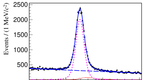
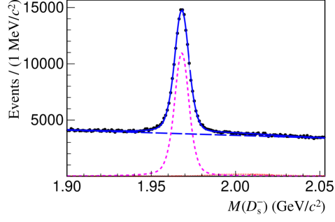
Figure 1: The invariant mass $M(D^{-}_{s})$ distributions for the ST modes $D^{-}_{s}\rightarrow K^{0}_{\scriptscriptstyle S}K^{-}$ (top) and $D^{-}_{s}\rightarrow K^{-}K^{+}\pi^{-}$ (bottom). Data (black points) are shown overlaid with the fit results including the total (solid blue), signal PDF (dashed magenta), $D^{-}$ background PDF (dotted red), and combinatorial background PDF (long-dashed blue) components.

Table 2: The ST yields and efficiencies for the two tag modes.

Tag mode	$N_{\rm ST}^{\alpha}$	$\epsilon_{\rm ST}^{\alpha}$
$D^{-}_{s}\rightarrow K^{0}_{\scriptscriptstyle S}K^{-}$	$\phantom{0}30673\pm 230$	46.3%
$D^{-}_{s}\rightarrow K^{-}K^{+}\pi^{-}$	$134370\pm 565$	38.8%

V Double Tag Analysis

In each event, once an ST $D^{-}_{s}$ candidate is found, three charged pions with the sum of charges opposite to the charge of the $D^{-}_{s}$ tag in the rest of the event (recoil side) are searched for. The tracking and PID requirements of charged pions are the same as those in the tag side as described in Sec. IV.

There are two major background sources that contribute to the $3\pi$ inclusive final states. The first source of background contribution is due to events with three correctly identified charged pions where at least one of them comes from $K^{0}_{\scriptscriptstyle S}\rightarrow\pi^{+}\pi^{-}$ decays. The other type of background comes from events for which at least one charged pion is misidentified. These two types of background sources are studied separately using dedicated MC simulations of inclusive $D^{+}_{s}$ decays to determine additional selection criteria, and to estimate the remaining contribution after imposing all the requirements. The background subtracted pion momentum spectra and mass spectra from the $3\pi$ system for the tag mode $D^{-}_{s}\rightarrow K^{-}K^{+}\pi^{-}$ are shown in Figs. 2 and 3, while the spectra for the tag mode $D^{-}_{s}\rightarrow K^{0}_{\scriptscriptstyle S}K^{-}$ follow very similar patterns with lower yields. There is reasonable agreement between data and the simulated sample, and any differences in the pion momentum spectra are later considered as a source of systematic uncertainties.

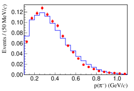
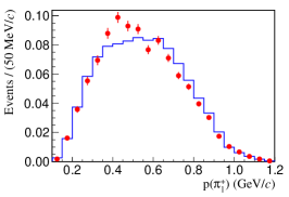
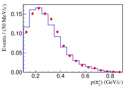
Figure 2: Normalized momentum spectra after background subtraction from the $3\pi$ system of the inclusive decay $D^{+}_{s}\rightarrow\pi^{+}\pi^{+}\pi^{-}X$ for the tag mode $D^{-}_{s}\rightarrow K^{-}K^{+}\pi^{-}$. The points are obtained from data and the solid line histograms are from inclusive MC simulation samples. The subscripts for $\pi^{+}$s indicate the order $p(\pi_{1}^{+})>p(\pi_{2}^{+})$.

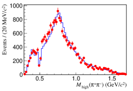
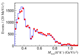
Figure 3: Normalized invariant mass spectra after background subtraction from the $3\pi$ system of the inclusive decay $D^{+}_{s}\rightarrow\pi^{+}\pi^{+}\pi^{-}X$ for the tag mode $D^{-}_{s}\rightarrow K^{-}K^{+}\pi^{-}$. The points are obtained from data and the solid line histograms are from inclusive MC simulation samples. The subscripts for the two $\pi^{+}\pi^{-}$ combinations indicate the order $M_{\rm high}(\pi^{+}\pi^{-})>M_{\rm low}(\pi^{+}\pi^{-})$. The dips in the $M(\pi^{+}\pi^{-})$ spectra are due to the 10 ${\mathrm{\,Me\kern-1.00006ptV\!/}c^{2}}$ $K^{0}_{\scriptscriptstyle S}$ mass veto defined in Sec. V.1.

V.1 Background from $K^{0}_{\scriptscriptstyle S}$ decays

To suppress the background contribution due to $K^{0}_{\scriptscriptstyle S}$ decays, each of the three charged pions of the $3\pi$ system is checked against a list of $K^{0}_{\scriptscriptstyle S}$ candidates in an event. Each of the $K^{0}_{\scriptscriptstyle S}$ candidates is reconstructed with the criteria defined in Sec. IV . If at least one pion is part of one reconstructed $K^{0}_{\scriptscriptstyle S}$ candidate that has $L/\sigma_{L}>2$ ($L$ is defined as the distance between the $K^{0}_{\scriptscriptstyle S}$ vertex and the IP, and $\sigma_{L}$ is the uncertainty of $L$), or within the mass window $|M(\pi^{+}\pi^{-})-m_{K^{0}_{\scriptscriptstyle S}}|<10$${\mathrm{\,Me\kern-1.00006ptV\!/}c^{2}}$, this signal candidate is rejected. With this requirement, about 88% of the $K^{0}_{\scriptscriptstyle S}$ meson related background contributions are rejected, while losing about 11% of the signal events.

V.2 Particle misidentification background

For one charged pion, there are three possible misID scenarios:

• $\mu^{\pm}\rightarrow\pi^{\pm}$,

• $e^{\pm}\rightarrow\pi^{\pm}$,

• $K^{\pm}\rightarrow\pi^{\pm}$.

As the charged pions are identified against kaons, the main misID background contributions are from the semileptonic $D^{+}_{s}$ decays, and the misidentified pion in the $3\pi$ system has the same charge as the signal $D^{+}_{s}$ side. Electron background can be largely removed by rejecting signal candidates for which at least one $e^{+}$ has been identified at the signal $D^{+}_{s}$ side. The electron PID is based on the likelihoods for the electron, pion, and kaon hypotheses ${\cal L}(h)(h=e,\pi,K)$ using information from the MDC, TOF, and EMC, as in Ref. BESIIIDs2eX . With this, about 90% of the $e^{+}\rightarrow\pi^{+}$ misID background contributions are removed at the cost of mere $\sim$5% of the signal events. The residual misID backgrounds are then dominated by the semimuonic decays $D^{+}_{s}\rightarrow X\mu^{+}\nu_{\mu}$, and are estimated from the $D_{s}$ inclusive MC simulation sample ($\sim$70%), , and the related systematic uncertainties are discussed in Sec. V.2.

V.3 Partial branching fractions

The $D^{+}_{s}\rightarrow\pi^{+}\pi^{+}\pi^{-}X$ partial BFs are measured in eleven $M(\pi^{+}\pi^{+}\pi^{-})$ intervals. The intervals are populated with approximately equal numbers of DT candidates, except for the last interval, where the signal candidates are predominantly from the exclusive decay of $D^{+}_{s}\rightarrow\pi^{+}\pi^{+}\pi^{-}$. The interval boundaries in the $M(\pi^{+}\pi^{+}\pi^{-})$ distribution are chosen as [0.40, 0.74, 0.90, 0.99, 1.08, 1.15, 1.23, 1.30, 1.41, 1.57, 1.90, 2.05] ${\mathrm{\,Ge\kern-1.00006ptV\!/}c^{2}}$.

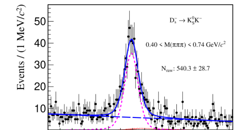
Figure 4: The $M(D^{-}_{s})$ distributions in the first $M(\pi^{+}\pi^{+}\pi^{-})$ interval for the tag modes of $D^{-}_{s}\rightarrow K^{0}_{\scriptscriptstyle S}K^{-}$ (top) and $D^{-}_{s}\rightarrow K^{-}K^{+}\pi^{-}$ (bottom). Data (black points) are shown overlaid with the fit results including the total (solid blue), signal PDF (dashed magenta), $D^{-}$ background PDF (dotted red), and combinatorial background PDF (long-dashed blue) components.

The number of $D^{+}_{s}\rightarrow\pi^{+}\pi^{+}\pi^{-}X$ signal candidates in each $M(\pi^{+}\pi^{+}\pi^{-})$ interval is determined by fitting the corresponding $M(D^{-}_{s})$ distribution of the tag side. From this fit, the raw signal yield $N^{\alpha}_{{\rm raw},i}$ is measured for each interval $i$ of the $M(\pi^{+}\pi^{+}\pi^{-})$ distribution, for tag mode $\alpha$. The signal shape for each tag mode is determined in the corresponding ST fit (results shown in Fig. 1). The same shape is used in all $M(\pi^{+}\pi^{+}\pi^{-})$ intervals, and the linear background shape parameter is left unconstrained in the fit. The fitted raw signal yields ($N^{\alpha}_{{\rm raw},i}$) are presented in Tables 3 and 4 for the tag modes of $D^{-}_{s}\rightarrow K^{0}_{\scriptscriptstyle S}K^{-}$ and $D^{-}_{s}\rightarrow K^{-}K^{+}\pi^{-}$, respectively. Two examples of the 22 fits are shown in Fig. 4, and the full set of fit results is made available as Supplemental Material supp . Tables 3 and 4 summarize the observed signal yields, after subtracting the $K^{0}_{\scriptscriptstyle S}$-decay related and misID background contributions from the raw signal yields as described earlier in this section.

Table 3: Raw signal yields and estimated background contributions for $D_{s}^{-}\rightarrow K^{0}_{\scriptscriptstyle S}K^{-}$ versus $D^{+}_{s}\rightarrow\pi^{+}\pi^{+}\pi^{-}X$ events. The associated uncertainties are statistical only. The uncertainties from different background contributions are due to the limited size of our inclusive MC simulation samples, whose integrated luminosity is 40 times of data.

$M(\pi^{+}\pi^{+}\pi^{-})$ interval	1	2	3	4	5	6
Raw yield	540.3 $\pm$ 28.7	625.9 $\pm$ 31.8	514.4 $\pm$ 28.4	627.7 $\pm$ 31.3	418.8 $\pm$ 26.1	486.8 $\pm$ 27.2
$K^{0}_{\scriptscriptstyle S}$ contribution	16.6 $\pm$ 0.7	37.9 $\pm$ 1.0	28.3 $\pm$ 0.9	22.4 $\pm$ 0.8	12.3 $\pm$ 0.6	11.3 $\pm$ 0.6
MisID contribution	40.7 $\pm$ 1.1	64.1 $\pm$ 1.4	44.8 $\pm$ 1.1	46.8 $\pm$ 1.2	35.5 $\pm$ 1.0	36.3 $\pm$ 1.0
Total background	57.4 $\pm$ 1.3	102.0 $\pm$ 1.70	73.1 $\pm$ 1.5	69.2 $\pm$ 1.4	47.7 $\pm$ 1.2	47.6 $\pm$ 1.2
Background subtracted yield	482.9 $\pm$ 28.8	523.9 $\pm$ 31.8	441.3 $\pm$ 28.4	558.5 $\pm$ 31.3	371.0 $\pm$ 26.1	439.2 $\pm$ 27.2
$M(\pi^{+}\pi^{+}\pi^{-})$ interval	7	8	9	10	11
Raw yield	403.3 $\pm$ 24.4	515.3 $\pm$ 27.8	400.5 $\pm$ 25.4	494.8 $\pm$ 27.4	153.3 $\pm$ 14.4
$K^{0}_{\scriptscriptstyle S}$ contribution	06.8 $\pm$ 0.4	09.7 $\pm$ 0.5	08.1 $\pm$ 0.5	02.7 $\pm$ 0.3	00.4 $\pm$ 0.1
MisID contribution	28.5 $\pm$ 0.9	35.9 $\pm$ 1.0	36.5 $\pm$ 1.0	27.6 $\pm$ 0.9	00.8 $\pm$ 0.2
Total background	35.3 $\pm$ 1.0	45.6 $\pm$ 1.1	44.6 $\pm$ 1.1	30.3 $\pm$ 0.9	01.3 $\pm$ 0.2
Background subtracted yield	368.1 $\pm$ 24.4	469.6 $\pm$ 27.8	356.0 $\pm$ 25.4	464.5 $\pm$ 27.4	152.0 $\pm$ 14.4

Table 4: Raw signal yields and estimated background contributions for $D_{s}^{-}\rightarrow K^{-}K^{+}\pi^{-}$ versus $D^{+}_{s}\rightarrow\pi^{+}\pi^{+}\pi^{-}X$ events. The associated uncertainties are statistical only. The uncertainties from different background contributions are due to the limited size of our inclusive MC simulation samples, whose integrated luminosity is 40 times of data.

$M(\pi^{+}\pi^{+}\pi^{-})$ interval	1	2	3	4	5	6
Raw yield	2300.8 $\pm$ 71.1	2883.4 $\pm$ 85.8	2405.7 $\pm$ 77.6	2630.0 $\pm$ 81.3	1944.3 $\pm$ 70.6	2276.2 $\pm$ 74.3
$K^{0}_{\scriptscriptstyle S}$ contribution	059.1 $\pm$ 1.3	148.2 $\pm$ 2.1	115.0 $\pm$ 1.8	093.6 $\pm$ 1.7	047.7 $\pm$ 1.2	048.4 $\pm$ 1.2
MisID contribution	190.1 $\pm$ 2.4	297.3 $\pm$ 3.0	214.6 $\pm$ 2.5	226.6 $\pm$ 2.6	164.3 $\pm$ 2.2	171.8 $\pm$ 2.2
Total background	249.2 $\pm$ 2.7	445.5 $\pm$ 3.6	329.6 $\pm$ 3.1	320.2 $\pm$ 3.1	212.0 $\pm$ 2.5	220.2 $\pm$ 2.5
Background subtracted yield	2051.6 $\pm$ 71.1	2437.9 $\pm$ 85.9	2076.1 $\pm$ 77.7	2309.8 $\pm$ 81.4	1732.2 $\pm$ 70.7	2056.0 $\pm$ 74.4
$M(\pi^{+}\pi^{+}\pi^{-})$ interval	7	8	9	10	11
Raw yield	1924.3 $\pm$ 65.2	2182.5 $\pm$ 68.8	1926.0 $\pm$ 65.5	1993.0 $\pm$ 63.7	767.7 $\pm$ 34.0
$K^{0}_{\scriptscriptstyle S}$ contribution	031.1 $\pm$ 1.0	036.9 $\pm$ 1.0	031.1 $\pm$ 1.0	010.7 $\pm$ 0.6	01.4 $\pm$ 0.2
MisID contribution	127.5 $\pm$ 1.9	169.0 $\pm$ 2.2	168.3 $\pm$ 2.2	126.3 $\pm$ 1.9	03.9 $\pm$ 0.3
Total background	158.7 $\pm$ 2.2	205.9 $\pm$ 2.5	199.4 $\pm$ 2.4	137.0 $\pm$ 2.0	05.3 $\pm$ 0.4
Background subtracted yield	1765.6 $\pm$ 65.2	1976.6 $\pm$ 68.8	1726.6 $\pm$ 65.5	1856.0 $\pm$ 63.7	762.4 $\pm$ 34.0

Using the observed signal yields and the efficiency matrix elements $\epsilon^{\alpha}_{ij}$ presented in Tables 5 and 6, the partial BFs in various $M(\pi^{+}\pi^{+}\pi^{-})$ intervals are calculated using Eqs. 4 and 6 and shown in Table 7 after combining the measurements from both tag modes.

Table 5: Efficiency matrix $\epsilon_{ij}$ in percentage for $D_{s}^{-}\rightarrow K^{0}_{\scriptscriptstyle S}K^{-}$ versus $D^{+}_{s}\rightarrow\pi^{+}\pi^{+}\pi^{-}X$ determined from signal MC simulated events. Each column gives the true $M(\pi^{+}\pi^{+}\pi^{-})$ interval $j$, while each row gives the reconstructed $M(\pi^{+}\pi^{+}\pi^{-})$ interval $i$.

$\epsilon_{ij}$	1	2	3	4	5	6	7	8	9	10	11
1	15.11	00.25	00.00	00.00	00.00	00.00	00.00	00.00	00.00	00.00	00.00
2	00.19	15.86	00.67	00.08	00.01	00.00	00.00	00.00	00.00	00.00	00.00
3	00.01	00.41	16.76	00.85	00.12	00.03	00.01	00.00	00.00	00.01	00.00
4	00.01	00.02	00.62	20.99	01.00	00.19	00.05	00.01	00.00	00.00	00.00
5	00.01	00.01	00.02	00.73	21.76	00.98	00.13	00.05	00.01	00.00	00.00
6	00.00	00.00	00.01	00.03	00.88	21.93	01.18	00.21	00.05	00.00	00.00
7	00.00	00.00	00.00	00.01	00.04	00.90	22.46	00.91	00.11	00.00	00.00
8	00.00	00.00	00.00	00.00	00.01	00.06	01.11	23.46	00.88	00.05	00.00
9	00.00	00.00	00.00	00.00	00.00	00.01	00.03	00.66	24.84	00.77	00.02
10	00.00	00.00	00.00	00.00	00.00	00.00	00.00	00.01	00.48	27.10	00.75
11	00.00	00.00	00.00	00.00	00.00	00.00	00.00	00.00	00.00	00.10	24.53

Table 6: Efficiency matrix $\epsilon_{ij}$ in percentage for $D_{s}^{-}\rightarrow K^{-}K^{+}\pi^{-}$ versus $D^{+}_{s}\rightarrow\pi^{+}\pi^{+}\pi^{-}X$ determined from signal MC simulated events. Each column gives the true $M(\pi^{+}\pi^{+}\pi^{-})$ interval $j$, while each row gives the reconstructed $M(\pi^{+}\pi^{+}\pi^{-})$ interval $i$.

$\epsilon_{ij}$	1	2	3	4	5	6	7	8	9	10	11
1	12.80	00.20	00.00	00.00	00.00	00.00	00.00	00.00	00.00	00.00	00.00
2	00.17	13.65	00.54	00.06	00.01	00.00	00.00	00.00	00.00	00.00	00.00
3	00.01	00.33	14.64	00.67	00.09	00.02	00.00	00.00	00.00	00.00	00.00
4	00.00	00.01	00.47	17.96	00.96	00.14	00.04	00.01	00.00	00.00	00.00
5	00.00	00.00	00.01	00.62	18.36	00.83	00.13	00.05	00.00	00.00	00.00
6	00.00	00.00	00.01	00.03	00.83	18.89	01.01	00.16	00.04	00.00	00.00
7	00.00	00.00	00.00	00.01	00.03	00.75	19.19	00.77	00.09	00.01	00.00
8	00.00	00.00	00.00	00.00	00.01	00.06	00.88	20.16	00.76	00.06	00.00
9	00.00	00.00	00.00	00.00	00.00	00.01	00.02	00.56	21.15	00.55	00.01
10	00.00	00.00	00.00	00.00	00.00	00.00	00.00	00.01	00.40	23.13	00.67
11	00.00	00.00	00.00	00.00	00.00	00.00	00.00	00.00	00.00	00.07	21.29

Table 7: Partial BFs (in percentage) of the decay $D^{+}_{s}\rightarrow\pi^{+}\pi^{+}\pi^{-}X$ combined from the two tag modes. The first and second uncertainties are statistical and systematic, respectively.

$M(\pi^{+}\pi^{+}\pi^{-})$ interval	${\Delta{\cal B}}_{3\pi X,i}$ (%)
1	$4.63\pm 0.14\pm 0.14$
2	$4.92\pm 0.16\pm 0.19$
3	$3.79\pm 0.13\pm 0.10$
4	$3.55\pm 0.12\pm 0.09$
5	$2.42\pm 0.10\pm 0.07$
6	$2.87\pm 0.10\pm 0.09$
7	$2.39\pm 0.09\pm 0.07$
8	$2.69\pm 0.09\pm 0.07$
9	$2.19\pm 0.08\pm 0.05$
10	$2.32\pm 0.07\pm 0.05$
11	$1.01\pm 0.04\pm 0.04$

VI Systematic uncertainties

The methods to determine the systematic uncertainties in the measured total and partial BFs of inclusive $D^{+}_{s}\rightarrow\pi^{+}\pi^{+}\pi^{-}X$ decays are described below.

VI.1 Signal shape in $M(D^{-}_{s})$

The signal $M(D^{-}_{s})$ PDF is changed from the DSCB shape to a shape modeled with signal MC simulated events convolved with a Gaussian function. The width and mean parameters of the Gaussian function are floating in the fits to account for the resolution difference between data and simulation. Alternatively, the fits are performed by allowing the two signal shape parameters $m_{0}$ and $\sigma_{0}$ in different $M(\pi^{+}\pi^{+}\pi^{-})$ intervals to differ. The largest variations are taken as the relative systematic uncertainties.

VI.2 Background shape in $M(D^{-}_{s})$

The background shape is changed from the linear PDF to an exponential or a histogram PDF based on MC simulation. Also the fits are performed with the yields of $D^{-}\rightarrow K^{0}_{\scriptscriptstyle S}\pi^{-}$ ($D^{-}\rightarrow K^{+}\pi^{-}\pi^{-}$) in the tag mode $D^{-}_{s}\rightarrow K^{0}_{\scriptscriptstyle S}K^{-}$ ($D^{-}_{s}\rightarrow K^{-}K^{+}\pi^{-}$) floating, rather than fixed to the numbers from simulation. The largest variations are taken as the relative systematic uncertainties.

VI.3 Pion tracking and PID efficiency

The $\pi^{\pm}$ tracking efficiency is studied with the control sample of $e^{+}e^{-}\rightarrow K^{+}K^{-}\pi^{+}\pi^{-}$ decay. The data-MC tracking efficiency ratios of $\pi^{+}$ and $\pi^{-}$ are measured in bins of pion transverse momentum. The signal MC samples are then weighted by these ratios to recalculate signal efficiency matrices. This leads to 0.98% variation in total BF, which is taken as the systematic uncertainty associated with tracking efficiency.

The $\pi^{\pm}$ PID efficiency is studied with the control samples of $e^{+}e^{-}\rightarrow K^{+}K^{-}\pi^{+}\pi^{-}(\pi^{0})$ and $\pi^{+}\pi^{-}\pi^{+}\pi^{-}(\pi^{0})$ decays. The data-MC tracking efficiency ratios of $\pi^{\pm}$ are measured in bins of pion momentum. The signal MC samples are then weighted by these ratios to recalculate signal efficiency matrices. This leads to 0.99% variation in the total BF, which is taken as the systematic uncertainty associated with PID efficiency.

VI.4 Background from $K^{0}_{\scriptscriptstyle S}$ decays

As $N^{\alpha}_{{K^{0}_{\scriptscriptstyle S}},i}$ defined in Eq. (3) is determined by the $D_{s}$ inclusive MC simulation sample, the data and simulation differences on the $D^{+}_{s}\rightarrow K^{0}_{\scriptscriptstyle S}\pi^{+}X$ contributions are studied by using control samples with dedicated stringent requirements on the $3\pi$ system: one $\pi^{+}\pi^{-}$ pair forms the reconstructed $K^{0}_{\scriptscriptstyle S}$ that has $L/\sigma_{L}>2$ and $|M(\pi^{+}\pi^{-})-m_{K^{0}_{\scriptscriptstyle S}}|<10$${\mathrm{\,Me\kern-1.00006ptV\!/}c^{2}}$. These requirements lead to a data sample with more than 99% of the $D^{+}_{s}$ candidates having a $\pi^{+}\pi^{-}$ pair from $K^{0}_{\scriptscriptstyle S}$. The agreement on the observed number of $D^{+}_{s}$ candidates in data and the number from simulation is at $\sim$10% level across different $M(\pi^{+}\pi^{+}\pi^{-})$ intervals. Therefore, the $N^{\alpha}_{{K^{0}_{\scriptscriptstyle S}},i}$ values are all scaled by $\pm 10$% in turn, and the BFs are recalculated according to altered $N^{\alpha}_{{\rm obs},i}$ values based on Eq. (3). The larger variations from the two measurements are taken as the relative systematic uncertainties on the $K^{0}_{\scriptscriptstyle S}$ background.

Furthermore, the systematic uncertainty related to the $K^{0}_{\scriptscriptstyle S}$ veto of $|M(\pi^{+}\pi^{-})-m_{K^{0}_{\scriptscriptstyle S}}|<10$ ${\mathrm{\,Me\kern-1.00006ptV\!/}c^{2}}$  is examined by varying the mass window by $\pm 5$ ${\mathrm{\,Me\kern-1.00006ptV\!/}c^{2}}$. The resulting changes in the BFs are smaller than the statistical uncertainties on the differences, so no uncertainty is assigned for this source according to Ref. barlow .

VI.5 Particle misidentification background

The $D_{s}$ inclusive MC simulation sample is also used to estimate $N^{\alpha}_{{\rm misID},i}$ defined in Eq. (3). The uncertainties on $N^{\alpha}_{{\rm misID},i}$ come from limited knowledge on the BFs of different decays that contribute to the misID backgrounds, and differences in misID rates between data and simulation, that are considered separately in the three misID scenarios as listed in Sec. V.2.

The $D^{+}_{s}\rightarrow\pi^{+}\pi^{-}\ell^{+}X$ decays form the background where the leptons $\ell=e,\mu$ are misidentified as pions, and the decays $D^{+}_{s}\rightarrow K^{-}\pi^{+}\pi^{+}X$ and $D^{+}_{s}\rightarrow K^{+}\pi^{+}\pi^{-}X$ are relevant for the background when a kaon is misidentified instead. The $D^{+}_{s}\rightarrow\pi^{+}\pi^{-}\ell^{+}X$ decays are dominated by the semileptonic decays of $D^{+}_{s}\rightarrow\phi\ell^{+}\nu_{\ell}$ and $D^{+}_{s}\rightarrow\eta^{(\prime)}\ell^{+}\nu_{\ell}$. By assuming LFU in semileptonic charm decays, the data and simulation differences on modeling the $D^{+}_{s}\rightarrow\pi^{+}\pi^{-}\ell^{+}X$ decays are studied using samples of $D^{+}_{s}\rightarrow\pi^{+}\pi^{-}e^{+}X$. This LFU assumption has been found to hold experimentally, e.g. within a precision of 1.4% in $D^{0}\rightarrow K^{-}\ell^{+}\nu_{\ell}$ decays bes3d2klnu . The electron PID requirement used on one of the positively charged track in the 3$\pi$ system is the same as that in Ref. BESIIIDs2eX . As the relative difference between data and MC simulation is below 5%, the sums of $N^{\alpha}_{e\rightarrow\pi,\ i}+N^{\alpha}_{\mu\rightarrow\pi,\ i}$ are all scaled by $\pm$5% in turn. The larger variations from the two measurements are taken as the systematic uncertainties related to the lepton misID background. Similarly, the dedicated simulation samples of $D^{+}_{s}\rightarrow K^{-}\pi^{+}\pi^{+}X$ and $D^{+}_{s}\rightarrow K^{+}\pi^{+}\pi^{-}X$ decays can be compared to data by imposing kaon identification requirements on one track from the 3$\pi$ system. This study indicates a disagreement between data and simulation at a level of about 15%. This is significantly larger than in the lepton case due to the poor knowledge of hadronic $D^{+}_{s}$ decays with at least one charged kaon. The $N^{\alpha}_{K\rightarrow\pi,\ i}$ values are all scaled by $\pm$15% in turn, and the larger variations from the two measurements are taken as the systematic uncertainties related to the kaon misID. Separate studies on the probabilities of tracks being misidentified as pions show the effects due to data and simulation differences are negligible. Therefore, this is not included as part of the systematic uncertainties.

VI.6 Pion multiplicity

The number of charged pions in $D^{+}_{s}\rightarrow\pi^{+}\pi^{+}\pi^{-}X$ decays may be inaccurately modeled in the simulation mainly due to the limited knowledge of hadronic $D^{+}_{s}$ decays with five or more charged pions in the final states such as $D^{+}_{s}\rightarrow\pi^{+}\pi^{+}\pi^{-}\pi^{+}\pi^{-}\pi^{0}(\pi^{0})$ pdg . The signal MC simulated events are weighted so that the simulated distribution of the number of charged pion candidates at the signal side matches with that in the data. This causes changes in signal efficiencies, and the resulting BF variations using the weighted MC simulated events are taken as the relative systematic uncertainties.

VI.7 Pion momenta

The signal MC simulated events are weighted to improve the agreement of the pion momentum distributions between data and simulation. The multivariate algorithm gbrw to determine the weights is trained on the distributions from unweighted signal MC simulation and background subtracted data samples as shown in Fig. 2. Using the weighted MC candidates based on the three-dimensional weighting scheme to recalculate signal efficiency matrices for both tag modes, the variations in the BF central values are taken as the relative systematic uncertainties.

As the data-MC differences in the angular distributions of pion momenta may result in differences in the mass spectra of the 3$\pi$ system, we also adopt a five-dimensional weighting scheme with the addition of $M_{\rm high}(\pi^{+}\pi^{-})$ and $M_{\rm low}(\pi^{+}\pi^{-})$ to account for the data-MC differences shown in Fig. 3. The resulting variations in BFs are smaller than those from the three-dimensional weighting scheme, and thus no additional uncertainty is assigned.

VI.8 Monte Carlo simulation sample size

The BFs are recalculated 1000 times by randomly perturbing the efficiency matrix elements shown in Tables 5 and 6 according to their uncertainties. The distributions of the recalculated BF central values are fitted with a Gaussian function and the fitted Gaussian widths are taken as the relative systematic uncertainties.

VI.9 Measurement bias

The uncertainties due to the entire analysis procedure to extract the BFs are estimated by using 40 inclusive MC simulation samples, each with a total candidate number statistically matched to that in the data. While good agreement between the input and measured BF values is found, the mean biases are taken as the relative systematic uncertainties.

VI.10 Signal MC simulation model

The purpose of measuring ${\cal B}(D^{+}_{s}\rightarrow\pi^{+}\pi^{+}\pi^{-}X)$ in intervals of $M(\pi^{+}\pi^{+}\pi^{-})$ is to be independent of the $D^{+}_{s}$ decay model used in the signal simulation. A number of exclusive $D^{+}_{s}$ decay modes such as $D^{+}_{s}\rightarrow\eta^{\prime}\rho^{+}$, $D^{+}_{s}\rightarrow\phi\pi^{+}\pi^{+}\pi^{-}$, and $D^{+}_{s}\rightarrow\phi\rho^{+}$ are used to perform the tests. The yield of the respective signal MC simulation events is weighted by about 40%. This in effect changes the related input BF by about 40% (up or down). The signal efficiency matrices are then updated based on the weighted MC simulation samples. The obtained BF results show good agreement with the baseline results well within one standard deviation. Therefore, a systematic uncertainty related to the signal MC simulation model is not assigned.

VI.11 Single-candidate requirement

The single-candidate requirement described in Sec. IV may bias the measurement due to potentially different candidate multiplicities and $M_{\rm rec}$ distributions in data and MC simulation. The systematic uncertainties from the single-candidate requirement are examined by rerunning the measurement with this requirement removed. The resulting BF variations are smaller than the statistical uncertainties on the differences, so no uncertainty is assigned for this source.

VI.12 Summary of systematic uncertainties

Table 8 summarizes contributions from the different systematic sources in the measurement of ${\cal B}(D^{+}_{s}\rightarrow\pi^{+}\pi^{+}\pi^{-}X)$. The largest sources of systematic uncertainties come from tracking and PID of the $3\pi$ system. These contributions are combined in quadrature to determine the total systematic uncertainty in the BF measurement. The summary table for the systematic uncertainties of the partial BFs of $D^{+}_{s}\rightarrow\pi^{+}\pi^{+}\pi^{-}X$ is given in the Supplemental Material supp .

Table 8: Sources of systematic uncertainties in the measurement of ${\cal B}(D^{+}_{s}\rightarrow\pi^{+}\pi^{+}\pi^{-}X)$.

Source	Relative uncertainty (%)
Signal shape	0.49
Background shape	0.40
$\pi^{+}\pi^{+}\pi^{-}$ tracking efficiency	0.98
$\pi^{+}\pi^{+}\pi^{-}$ PID efficiency	0.99
$K^{0}_{\scriptscriptstyle S}$ background	0.34
Kaon misID background	0.32
Lepton misID background	0.35
Pion multiplicity	0.51
Pion momenta	0.86
MC simulation sample size	0.01
Fit bias	0.03
Total	1.92

VII Summary

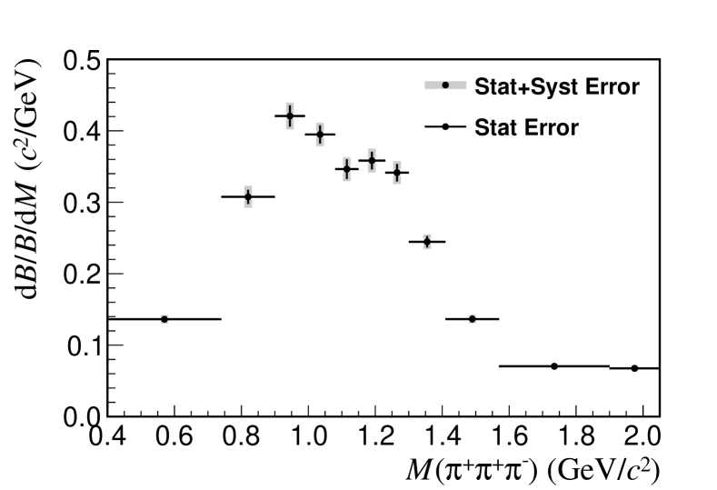
Figure 5: Partial BFs normalized by the total BF and interval widths as a function of $M(\pi^{+}\pi^{+}\pi^{-})$ for the $D^{+}_{s}\rightarrow\pi^{+}\pi^{+}\pi^{-}X$ decay. The vertical gray lines represent the uncertainties as the quadratic sums of the statistical and systematic uncertainties.

Based on 3.19 $\mbox{\,fb}^{-1}$ of $e^{+}e^{-}$ collision data recorded with the BESIII detector at $E_{\rm cm}=4.178$ $\mathrm{\,Ge\kern-1.00006ptV}$, the BF of the inclusive $D^{+}_{s}\rightarrow\pi^{+}\pi^{+}\pi^{-}X$ decay is measured for the first time. It is found to be

$${\cal B}(D^{+}_{s}\rightarrow\pi^{+}\pi^{+}\pi^{-}X)=\left(32.81\pm 0.35_{\rm stat}\pm{0.63}_{\rm syst}\right)\%.$$

This is larger than the sum of all observed exclusive BFs of $\sim$25% based on the PDG and recent measurements as summarized in Table 1, hinting at potentially unobserved decay modes with at least three charged pions in the final states.

Furthermore, the partial BFs of the $D^{+}_{s}\rightarrow\pi^{+}\pi^{+}\pi^{-}X$ decay as a function of $M(\pi^{+}\pi^{+}\pi^{-})$ are also measured, as presented in Table 7 and Fig. 5. As the feed-up contribution from lower intervals is expected to be negligible ($\sim$1% of exclusive signals), the partial BF in the last $M(\pi^{+}\pi^{+}\pi^{-})$ interval is consistent with the exclusive BF of ${\cal B}(D^{+}_{s}\rightarrow\pi^{+}\pi^{+}\pi^{-})=(1.08\pm 0.04)$% from the PDG pdg , with somewhat lower precision. The measured total and partial BFs of $D^{+}_{s}\rightarrow\pi^{+}\pi^{+}\pi^{-}X$ offer important inputs to constrain the systematic uncertainties in future LHCb measurements on $R(D^{*-})$ and $R(\mathchar 28931\relax_{c}^{+})$ with much larger data samples lhcb-white-paper .