Multi-Dimensional Quantum Walks:
a Playground of Dirac and Schrödinger Particles

Abstract

We propose a new multi-dimensional discrete-time quantum walk (DTQW), whose continuum limit is an extended multi-dimensional Dirac equation, which can be further mapped to the Schrödinger equation. We show in two ways that our DTQW is an excellent measure to investigate the two-dimensional (2D) extended Dirac Hamiltonian and higher-order topological materials. First, we show that the dynamics of our DTQW resembles that of a 2D Schrödinger harmonic oscillator. Second, we find in our DTQW topological features of the extended Dirac system. By manipulating the coin operators, we can generate not only standard edge states but also corner states.

I Introduction

The quantum walk is a quantum analogue of random walk. Instead of stochastic fluctuations of a classical random walker, a quantum walker moves under interference of quantum fluctuations at each site, which deterministically governs the walker’s dynamics. Quantum walk was originally introduced by Aharonov et al. Aharonov et al. (1993), who first referred to it as “quantum random walk.” Meyer Meyer (1996) built a systematic model and found a correspondence to Feynman’s path integral Feynman and Hibbs (1965) of the Dirac equation. Started by Farhi and Gutmann Farhi and Gutmann (1998), quantum walks have been well studied in the context of quantum information Ambainis et al. (2001); Asaka et al. (2021). To this day, studies of quantum walks have become even more interdisciplinary and extended over a variety of research fields, such as biophysics Engel et al. (2007); Dudhe et al. (2022) and condensed-matter physics Oka et al. (2005), particularly topological materials Kitagawa et al. (2010); Kitagawa (2012); Asbóth and Obuse (2013).

There are two types of time evolution: continuum-time quantum walks and discrete-time quantum walks (DTQW). We focus on the latter, in which the space and time are both discrete. Strauch Strauch (2006) showed that the continuum limit of the unitary time evolution of one-dimensional (1D) DTQW gives that of a Dirac particle. This correspondence of DTQW has enabled us to understand physical meaning of quantum walks better. Since squaring the Dirac Hamiltonian with a linear potential produces the Schrödinger Hamiltonian with a harmonic potential, we can make further correspondence between a quantum walker and a Schrödinger particle in 1D. However, such investigation has been limited to 1D systems. In two-dimensional (2D) systems, some quantum walks give a Dirac Hamiltonian in its continuum limit Di Franco et al. (2011); Bru et al. (2016); Arrighi et al. (2018), but there are usually only two internal states and hence one cannot obtain the 2D Schrödinger Hamiltonian by squaring it.

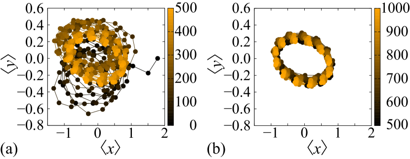
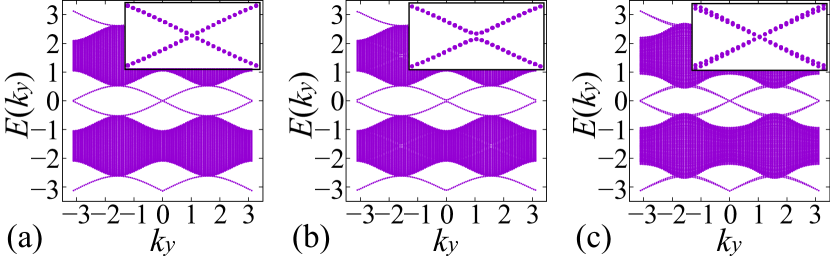
Figure 1: (Color online). The expectation values $\expectationvalue{x}$ and $\expectationvalue{y}$ of the position of 2D DTQW for (a) $0\leq T\leq 500$ and for (b) $500\leq T\leq 1000$. Black circles indicate the values at the beginning of time evolution; they turn into orange as time goes on. We set $\hbar=a=\Delta t=1$.

Figure 2: Dispersion relation of the quasi-energy spectra $E(k_{y})$ with $\theta_{1}=-\theta_{2}=\pi/3$. (a) $\theta_{y}=0$ and (b) $\theta_{y}=\pi/50$ without randomness, and (c) $\theta_{y}=0$ with randomness $\Delta{\theta_{x}}_{0}(x)\in[-0.25,0.25]$. The central part of the dispersion is enlarged in the upper right corner in each panel. We set $\hbar=a=\Delta t=1$.

In this paper, we show in two ways that our DTQW is an excellent measure to investigate an extended 2D Dirac Hamiltonian with additional internal degrees of freedom. We analyze its dynamics and topological properties, especially higher-order topological insulators Murani et al. (2017); Imhof et al. (2018); Peterson et al. (2018). We start with proposing a 2D extended Dirac Hamiltonian

$$H_{\mathrm{D}}^{(2)}:=H_{\mathrm{D}_{x}}\otimes\tau^{0}+\sigma^{x}\otimes H_{\mathrm{D}_{y}}$$

$$:=\quantity(\epsilon\sigma^{z}p_{x}+m_{x}(x)\sigma^{y})\otimes\tau^{0}+\sigma^{x}\otimes\quantity(\epsilon\tau^{z}p_{y}+m_{y}(y)\tau^{y}).$$ (1)

that can be mapped to a 2D DTQW as well as to a Schrödinger Hamiltonian as we will show below. Our key trick is to introduce $\sigma^{x}$ in the second term so that upon squaring the Hamiltonian (I) all crossing terms may vanish and the result can be the standard 2D Schrödinger Hamiltonian. With the additional internal degrees of freedom due to the introduction of $\sigma^{x}$, we refer to the Dirac Hamiltonian (I) as the extended Dirac Hamiltonian. The same applies to higher-dimensional cases; see Eq. (15) below for the three-dimensional (3D) case with the eight-dimensional internal degree of freedom.

Remember that the original 3D Dirac equation is written with a four-dimensional spinor degree of freedom, which Dirac assigned to a particle and an anti-particle each with a spin 1/2 degree of freedom. This is partly because the four-dimensional degree of freedom is the minimal representation of gamma matrices that satisfies the anticommutation relation necessary in deriving the Dirac equation from the Klein-Gordon equation; see e.g. Ref. Ryder (1996). However, it does not mean that we cannot go beyond Dirac’s minimal representation. As far as the dimensionality of the spinor degree of freedom is a multiple of four in the spatial three-dimensional case as in Eq. (15) below, it is possible to construct Dirac-type equations with additional internal degrees of freedom, which is what we have done here. Thus we refer to our model as the extended Dirac Hamiltonian.

As another point, we might have had to refer to the square of the Dirac Hamiltonian as the Klein-Gordon equation, but we will below refer to it as the Schrödinger Hamiltonian because we will demonstrate the behavior of a harmonic oscillator under the linear spacial dependence of the mass terms $m_{x}(x)$ and $m_{y}(y)$. Indeed, the existence of the two mass terms in Eq. (I) is also a new feature of our extended Dirac Hamiltonian.

The introduction of $\sigma^{x}$ in Eq. (I) also enables corner states, the second-order topological states, to emerge. The higher-order topological states has come under an intensive investigation in these days (see e.g. Refs. Murani et al. (2017); Imhof et al. (2018); Peterson et al. (2018); Benalcazar et al. (2017a); Hayashi (2018); Schindler et al. (2017); Langbehn et al. (2017); Song et al. (2017); Benalcazar et al. (2017b)). A systematic construction of Hamiltonians that harbors higher-order topological states has been developed recently by Hayashi Hayashi (2018). The extended Dirac Hamiltonian proposed in the present paper turns out to follow the construction of higher-order topological states, and hence the present two-dimensional DTQW explicitly exhibits corner states. In other words, the present DTQW models simulate quantum dynamics of higher-order topological insulators.

We numerically find that our 2D quantum walker behaves like a 2D harmonic oscillator as shown in Fig. 2, to which we will get back below. We also reveal nontrivial topological properties of our DTQW using the implication of the Dirac Hamiltonian Jackiw and Rebbi (1976). We also numerically find two different types of topological bound states, namely edge states of the topology of type $2\mathbb{Z}$ (which are robust against randomness in Fig. 2) and corner states, by manipulating the coin operators of our DTQW. (See below for the definitions of the notations in Figs. 2 and 2.)

I.1 Review of One-Dimensional Case

Let us first review the continuum limit of the 1D DTQW. We define the time evolution of the standard 1D quantum walk $\ket{\psi(T)}={U^{(1)}}^{T}\ket{\psi(0)}$ for $T\in\mathbbm{Z}$ in terms of the following coin and shift operators:

$$C :=\sum_{x\in a\mathbbm{Z}}\outerproduct{x}{x}\otimes\mathrm{e}^{-\mathrm{i}\theta_{x}(x)\sigma^{y}},$$ (2)

$$S :=\sum_{x\in a\mathbbm{Z}}(\outerproduct{x-a}{x}\otimes\outerproduct{\mathrm{L}}{\mathrm{L}}+\outerproduct{x+a}{x}\otimes\outerproduct{\mathrm{R}}{\mathrm{R}})$$ (3)

with $U^{(1)}:=SC$. Here, $\theta_{x}(x)$ is a coefficient set to a linear function of $x$ below, $a$ is the lattice constant and $\{\sigma^{x},\sigma^{y},\sigma^{z}\}$ are the Pauli matrices in the space spanned by the leftward state, $\ket{\mathrm{L}}=(1,0)^{\top}$, and the rightward state, $\ket{\mathrm{R}}=(0,1)^{\top}$. We set $\hbar$ to unity throughout the paper.

Let us express the shift operator (3) in the form

$$S=\exp\quantity(-a\sigma^{z}\derivative{x})=\exp(-\mathrm{i}a\sigma^{z}p_{x})$$ (4)

with $p_{x}=-i\derivative*{x}$. Scaling the parameters $a$ and $\theta_{x}(x)$ as in $\epsilon:=a/\Delta t$ and $m_{x}(x):=\theta_{x}(x)/\Delta t$ with $t:=T\Delta t$ and taking the limit $\Delta t\to 0$ with $T\to\infty$ under a fixed value of $t$, we find the continuum limit of the time-evolution operator in the form of the Trotter formula Strauch (2006)

$$\lim_{\Delta t\to 0}{U^{(1)}}^{T}=\lim_{\Delta t\rightarrow 0}\quantity[\mathrm{e}^{-\mathrm{i}\epsilon\Delta t\sigma^{z}p_{x}}\mathrm{e}^{-\mathrm{i}m_{x}(x)\Delta t\sigma^{y}}]^{T}=\mathrm{e}^{-\mathrm{i}H_{\mathrm{D}}^{(1)}t},$$ (5)

where

$$H_{\mathrm{D}}^{(1)}=\epsilon\sigma^{z}p_{x}+m_{x}(x)\sigma^{y}$$ (6)

represents the Hamiltonian of a Dirac particle with mass $m_{x}(x)$ in 1D. We can analyze its dynamics approximately by squaring it:

$${\matrixquantity(H_{\mathrm{D}}^{(1)})}^{2}=(\epsilon^{2}{p_{x}}^{2}+m_{x}(x)^{2})\sigma^{0}-\mathrm{i}\epsilon\sigma^{x}[p_{x},m_{x}(x)]=:H_{\mathrm{S}}^{(1)},$$ (7)

where $\sigma^{0}$ denotes the $2\times 2$ identity matrix for the space spanned by $\ket{\mathrm{L}}$ and $\ket{\mathrm{R}}$. Let us assume that $m_{x}(x)=\theta_{x}(x)/\Delta t$ is linear in $x$ as in $\theta_{x}(x)=bx$ and $m_{x}(x)=\beta x$ with $\beta=b/\Delta t$. This reduces the last term of $H_{\mathrm{S}}^{(1)}$ to $-\epsilon\beta\sigma^{x}$. A unitary transformation $V=\exp(\mathrm{i}\sigma^{y}\pi/4)$ turns the last term further to $\epsilon\beta\sigma^{z}$, diagonalizing the Hamiltonian $H_{\mathrm{S}}^{(1)}$ to the two blocks of

$$\tilde{H}_{\mathrm{S}_{\pm}}^{(1)}:=\epsilon^{2}{p_{x}}^{2}+\beta^{2}x^{2}\pm\epsilon\beta,$$ (8)

each of which is the Schrödinger Hamiltonian in a 1D harmonic potential with a constant term under the following identification:

$$\epsilon^{2}\leftrightarrow\frac{1}{2m_{\mathrm{S}}},\quad\beta^{2}\leftrightarrow\frac{m_{\mathrm{S}}\omega^{2}}{2},\quad\epsilon\beta\leftrightarrow\frac{\omega}{2}.$$ (9)

The preceding argument shows that the Dirac and Schrödinger Hamiltonians share the same eigenvectors. Indeed, the time evolution of $H_{\mathrm{D}}^{(1)}$ is approximately given by $\tilde{H}_{\mathrm{S}}^{(1)}$. We can numerically confirm that the Dirac Hamiltonian makes a wave packet oscillate around $x=0$ approximately like a harmonic oscillator.

II Two-Dimensional Model

Our first point of the paper is to extend the argument to higher dimensions. There have been two major kinds of 2D DTQW: the Grover walk Shenvi et al. (2003) and an alternative quantum walkDi Franco et al. (2011). However, we cannot map either of them to the Schrödinger equation. Instead of these two DTQWs, we here introduce a new DTQW whose continuum limit yields the extended Dirac Hamiltonian (I). Let $\ket{\mathrm{L}}$, $\ket{\mathrm{R}}$, $\ket{\mathrm{D}}$ and $\ket{\mathrm{U}}$ denote the basis vectors for the leftward, rightward, downward, and upward states, respectively. In Eq. (I), $\{\sigma^{x},\sigma^{y},\sigma^{z}\}$ are the the Pauli matrices for the space spanned by $\ket{\mathrm{L}}$ and $\ket{\mathrm{R}}$, while $\{\tau^{x},\tau^{y},\tau^{z}\}$ and $\tau^{0}$ are the Pauli matrices and the identity matrix for the space spanned by $\ket{\mathrm{D}}$ and $\ket{\mathrm{U}}$. We let $m_{x}(x)$ and $m_{y}(y)$ denote the mass terms. The momenta $p_{x}$ and $p_{y}$ can be rewritten in the forms of $-\mathrm{i}\partial/\partial x$ and $-\mathrm{i}\partial/\partial y$, respectively.

We can easily confirm that the extended Dirac Hamiltonian (I) is by squaring it mapped to the Schrödinger Hamiltonian

$$H_{\mathrm{S}}^{(2)}:=H_{\mathrm{S}_{x}}\otimes\tau^{0}+\sigma^{0}\otimes H_{\mathrm{S}_{y}},$$ (10)

where

$$H_{\mathrm{S}_{x}} :=(\epsilon^{2}{p_{x}}^{2}+m_{x}(x)^{2})\sigma_{0}-\mathrm{i}\epsilon\sigma^{x}\commutator{p_{x}}{m_{x}(x)},$$ (11)

$$H_{\mathrm{S}_{y}} :=(\epsilon^{2}{p_{y}}^{2}+m_{y}(y)^{2})\tau^{0}-\mathrm{i}\epsilon\tau^{x}\commutator{p_{y}}{m_{y}(y)}.$$ (12)

Assumptions

$$m_{x}(x)=\beta x\quad\mbox{and}\quad m_{y}(y)=\beta y$$ (13)

reduce Eq. (10) to

$$H_{\mathrm{S}}^{(2)} :=(\epsilon^{2}{p_{x}}^{2}+\beta^{2}x^{2}-\epsilon\beta\sigma^{x})\otimes\tau^{0}$$

$$+\sigma^{0}\otimes(\epsilon^{2}{p_{y}}^{2}+\beta^{2}y^{2}-\epsilon\beta\tau^{x}),$$ (14)

which represents a 2D harmonic oscillator under the identification (9).

We can further extend the argument into the 3D model with the extended Dirac Hamiltonian

$$H_{\mathrm{D}}^{(3)} :=H_{\mathrm{D}_{x}}\otimes\tau^{0}\otimes v^{0}+\sigma^{x}\otimes H_{\mathrm{D}_{y}}\otimes v^{0}+\sigma^{x}\otimes\tau^{x}\otimes H_{\mathrm{D}_{z}}$$ (15)

although it may not be a standard 3D Dirac Hamiltonian because we have now $2\times 2\times 2$ degrees of freedom at each site. In Eq. (15), $v^{0}$ is the identity matrix for the space spanned by the backward state $\ket{\mathrm{B}}$ and the forward state $\ket{\mathrm{F}}$ of the additional inner degree of freedom, while $\{v^{x},v^{y},v^{z}\}$ are the Pauli matrices for the same space. Extension to even higher dimensions should be obvious.

II.1 Two-Dimensional Oscillator

We next construct our DTQW model from the extended Dirac Hamiltonian (I). The Hilbert space for the inner degrees of freedom at each site is now spanned by

$$(\ket{\mathrm{L}}+\ket{\mathrm{R}})\oplus(\ket{\mathrm{D}}+\ket{\mathrm{U}})=\ket{\mathrm{LD}}+\ket{\mathrm{RD}}+\ket{\mathrm{LU}}+\ket{\mathrm{RU}}.$$ (16)

We hereafter fix the ordering of the basis vectors in this way. After conducting the Trotter decomposition on $\exp(-\mathrm{i}H_{\mathrm{D}}^{(2)}t)$, we obtain the time-evolution operator $U^{(2)}$ in the form of $U^{(2)}=S_{y}C_{y}S_{x}C_{x}$ with

$$\matrixquantity{C_{x}:=\mathrm{e}^{-\mathrm{i}\theta_{x}(x)(\sigma^{y}\otimes\tau^{0})},\quad S_{x}:=\mathrm{e}^{-a(\sigma^{z}\otimes\tau^{0})\partial_{x}},\\ C_{y}:=\mathrm{e}^{-\mathrm{i}\theta_{y}(y)(\sigma^{x}\otimes\tau^{y})},\quad S_{y}:=\mathrm{e}^{-a(\sigma^{x}\otimes\tau^{z})\partial_{y}}.}$$ (17)

Let us here assume that $\theta_{x}(x)$ and $\theta_{y}(y)$ are linear in $x$ and $y$, respectively, as in

$$\theta_{x}(x)=bx\quad\mbox{and}\quad\theta_{y}(y)=by,$$ (18)

which are related to Eq. (13) as in $\theta_{x}(x)=m_{x}(x)\Delta t$ and $\theta_{y}(y)=m_{y}(y)\Delta t$. We can regard this as effective linear potentials for the corresponding Dirac particle. The operators $C_{x}$ and $S_{x}$ in the $x$ direction are given by straightforwardly extending the corresponding operators (2) and (3) for the 1D DTQW, respectively. On the other hand, the operators $C_{y}$ and $S_{y}$ read

where

$$\matrixquantity{&c:=\cos{(by)},\quad s:=\sin{(by)},\\[2.0pt] &P:=\frac{1}{2}(\outerproduct{y-a}{y}+\outerproduct{y+a}{y}),\\[2.0pt] &Q:=\frac{1}{2}(\outerproduct{y-a}{y}-\outerproduct{y+a}{y}).}$$ (19)

These coin and shift operators in Eq. (II.1) look differently from the Grover walk Shenvi et al. (2003) and the alternative quantum walk Di Franco et al. (2011) because of the $\sigma^{x}$ term in the extended Dirac Hamiltonian (I). We believe our DTQW to be better in representing 2D physics in the sense that it exhibits dynamics of a 2D harmonic oscillator as we demonstrated in Fig. 2.

In the numerical calculation for Fig. 2, we set the system size to $L_{x}=L_{y}=101$ with $-50\leq x\leq 50$ and $-50\leq y\leq 50$ under periodic boundary conditions in both directions. We used the effective potential of the form

$$\theta_{x_{\mu}}(x_{\mu})=\begin{cases}\pi/4\quad&\mbox{for $5<x_{\mu}\leq 50$},\\ bx_{\mu}\quad&\mbox{for $\absolutevalue{x_{\mu}}\leq 5$},\\ -\pi/4\quad&\mbox{for $-50\leq x_{\mu}<-5$},\end{cases}$$ (20)

where $x_{1}=x$, $x_{2}=y$ and $b=\pi/20$. We repeated numerical multiplication of $U^{(2)}$ to the initial state. For the initial state, we used an eigenstate of the eigenvalue unity of the time-evolution operator $U^{(2)}$ shifted in the $x$ direction by two sites and imposed the initial velocity in the form of $\mathrm{e}^{\mathrm{i}(k_{x}x+k_{y}y)}$ with $(k_{x},k_{y})=(0,\pi)$. The eigenstate of the eigenvalue unity of $U^{(2)}$ is in the Trotter limit given by the Gaussian form of the zero-energy eigenvalue of our extended 2D Dirac Hamiltonian (I), which we explicitly obtain in App. LABEL:appendeigstate-linearpot-2D.

Figure 2 shows the expectation values,

$$\matrixquantity{\expectationvalue{x(T)}:=\sum_{x,y}xP(x,y,T),\\ \expectationvalue{y(T)}:=\sum_{x,y}yP(x,y,T),}$$ (21)

at each time step, where $P(x,y,T)$ is the quantum probability at site $(x,y)$ at time step $T$ and satisfies $\sum_{x,y}P(x,y,T)=1$. We observe the circular trajectory in Fig. 2; after some time it converges to an orbit of a limit cycle (Fig. 2(b)), which closely resembles the one of a Schrödinger dynamics under a 2D harmonic potential. In Fig. 3, we can see that the standard deviations almost converge to a constant after $T\sim 500$, which implies that the walker reaches a steady state of a circling wave packet around the time. With these facts, we believe that we successfully observe dynamics that resembles the 2D harmonic oscillator. We confirm in App. LABEL:appendeigstate-linearpot-2D that all the eigenstates of the corresponding 2D extended Dirac Hamiltonian (I) are composed of the eigenstates of a 2D harmonic oscillator.

The fact that the present 2D DTQW behaves like a 2D harmonic oscillator is particularly important to some of the present authors for studies of quantum active matter. They defined in Ref. Yamagishi et al. (2023) a quantum version of the active Brownian particle Schweitzer et al. (1998), in which Schweitzer et al. numerically demonstrated that a classical active particle climbs up the 2D harmonic potential and makes a circular orbit. Some of the present authors Yamagishi et al. (2023) are reproducing similar movement of the quantum version, using the present oscillator behavior of the 2D DTQW. This is why the present quantum walker’s making the circular orbit is critically important.

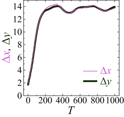
Figure 3: (Color online). The time-step dependence of the standard deviations $\Delta x$ (thin purple line) and $\Delta y$ (thick dark green line) of the quantum walker in 2D. We set $\hbar=a=\Delta t=1$.

II.2 Topological Edge States of Two-Dimensional DTQW

Let us turn to topological properties of DTQW. Jackiw and Rebbi Jackiw and Rebbi (1976) suggested that when a Dirac system e.g. Eq. (6) (presumed to be extended to infinity) has two domains in each of which the mass term takes a different value e.g.,

$$m_{x}(x)=\begin{cases}m_{1}\quad&\mbox{for $x>0$},\\ m_{2}\quad&\mbox{for $x<0$},\end{cases}$$ (22)

then a robust zero-energy state spatially localized in the vicinity of the domain wall emerges in the mass gap iff the sign of $m_{1}$ and $m_{2}$ differ Shen (2013). In other words, the zero-energy domain-wall state is protected by an index $\nu_{1}$ defined as $(-1)^{\nu_{1}}={\rm sgn}(m_{1}){\rm sgn}(m_{2})$, which takes two integral values $\nu_{1}=0,1$ in this particular case. Now that the concept of topological insulator is well established, Jackiw and Rebbi’s example is recognized as its earliest realization, and the index $\nu_{1}$ is interpreted as a topological number. Indeed, the model (6) belongs to the symmetry class DIII with the topology of type $\mathbb{Z}_{2}$ in 1D Kitaev (2009); Ryu et al. (2010).

We checked it numerically using the 1D DTQW prescribed by Eqs. (2) and (3) with $\theta_{x}(x)$ having two domains,

$$\theta_{x}(x)=\begin{cases}\theta_{1}\quad&\mbox{for $|x|<L_{1}$},\\ \theta_{2}\quad&\mbox{for $L_{1}<|x|<[L_{x}/2]$}.\end{cases}$$ (23)

Note that each of the domain walls at $x=\pm L_{1}$ corresponds to the one in Eq. (22) as in $\theta_{x}(x)=m_{x}(x)\Delta t$. Since our DTQW is under the periodic boundary condition, there are two domain walls with discontinuities in $m_{x}(x)$ at $x=\pm L_{1}$, and therefore we observed two topologically protected zero-energy states, each of which is localized at a different domain wall. (Incidentally, squaring the Dirac Hamiltonian as in Eq. (7), we find that the last term of $H_{\mathrm{S}}^{(1)}$ yields delta functions at the discontinuities of $m_{x}(x)$, and thus the edge states of the Dirac Hamiltonian can also be interpreted as bound states of the corresponding Schrödinger particle to the delta potentials.)

In the 2D realization of our DTQW prescribed by Eqs. (17) and (II.1), using again the domain-wall configuration of $\theta_{x}(x)$ introduced in the 1D case with $\theta_{y}(y)\equiv 0$ in Eq. (17), the protected zero-energy states acquire a dispersion; see App. LABEL:appendedge2D for the solution in the case of the 2D extended Dirac Hamiltonian (I). Figure 2(a) shows quasi-energy spectrum $E_{n}=-\mathrm{i}\log{U^{(2)}_{n}}$ for each ${k_{y}}_{n}=2n\pi/L_{y}$ with $\theta_{y}=0$. We observe that two linear dispersions with positive and negative slopes completely traverses the bulk energy gap, manifesting the feature of protected gapless edge states. Their gaplessness is protected by a topological number $\nu_{1}=1$ introduced above; when $\nu_{1}$ changes upon changing $\theta_{x}(x)$, the bulk energy gap must close once and reopen in the space of control parameters, where different topological phases are defined.

The extended Dirac Hamiltonian (I) with $m_{y}=0$ has a time-reversal symmetry under $\Theta=\sigma^{x}\otimes\tau^{y}K$ with $K$ being complex conjugation, a particle-hole symmetry under $\Xi=\mathbbm{I}_{4\times 4}K$, and a chiral symmetry under $\Pi=\sigma^{x}\otimes\tau^{y}$, and hence belongs to the symmetry class DIII with a topology of type $\mathbbm{Z}_{2}$ in 2D Kitaev (2009); Ryu et al. (2010). However, the time-evolution operator $U^{(2)}=S_{y}S_{x}C_{x}$ (with $\theta_{y}=0$) only has the particle-hole symmetry under $\Xi=\mathbbm{I}_{4\times 4}K$ because of the specific ordering of $S_{y}S_{x}$ ($\neq S_{x}S_{y}$), and hence our DTQW belongs to the symmetry class D with a topology of type $\mathbbm{Z}$ in 2D Kitaev (2009); Ryu et al. (2010). (Incidentally, we have an additional sublattice symmetry in $S_{y}$. Adding the phase $\mathrm{e}^{\mathrm{i}\pi}$ to the every other $y$ and shifting $k_{y}$ with $\pi$ do not change $S_{y}$. This results in a $\pi$-periodicity in $k_{y}$ in the spectra in Fig. 2.)

We can understand the structure of the dispersion of edge states in Fig. 2(a) as in Fig. 4.

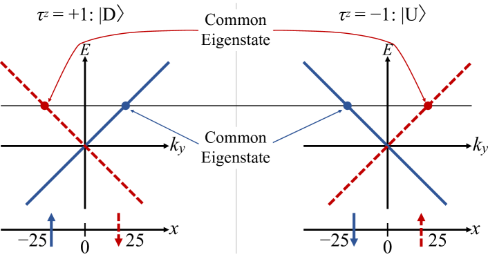
Figure 4: Schematic representation of the dispersion around $k_{y}=0$ in Fig. 2(a). We set $\hbar=a=\Delta t=1$.

Let us first note that our time-evolution operator $U^{(2)}=S_{y}S_{x}C_{x}$ for $\theta_{y}=0$ is block-diagonalized for the blocks $\tau^{z}=\pm 1$ with the same absolute value of $k_{y}$ but with a different sign. Since each block belongs to the class D, we have a topology of type $2\mathbbm{Z}$. In the block of $\tau^{z}=1$, namely $\ket{\mathrm{D}}$, an edge state localized at $x=-L_{1}=-25$ in Fig. 5 has the dispersion of a positive slope and one at $x=L_{1}=25$ has one with a negative slope as shown in Fig. 4.

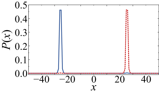
Figure 5: Probability density of an edge state localized around $x=-25$ (solid blue line) and one localized around $x=25$ (red broken line) with $k_{y}=0$ and the zero quasi-energy in the spectrum of Fig. 2(a). We set $\hbar=a=\Delta t=1$.

In the block of $\tau^{z}=-1$, namely $\ket{\mathrm{U}}$, on the other hand, an edge state at $x=-L_{1}=-25$ has the dispersion with a negative slope and the other at $x=L_{1}$ has one with a positive slope. Since the two blocks have opposite signs of $k_{y}$, the dispersion has a mirror symmetry, and hence the eigenstates on the two solid lines in Fig. 4 are common to each other; the same applies to the eigenstates on the broken lines. This is why we observe the lines with both positive and negative slope crossing at $k_{y}=0$. Two eigenvalues are degenerate on each line.

Upon introducing a nonzero value of $\theta_{y}$, which is incompatible with the dictated symmetry of class D, a gap emerges around $k_{y}=0$ as shown in Fig. 2(b). Meanwhile, the topological edge states are robust against other types of small perturbation, which we numerically confirm by introducing randomness. We added to $\theta_{x}(x)$ a random perturbation $\Delta{\theta_{x}}_{0}(x)$, randomly choosing independently for each site uniformly from the range $[-0.25,0.25]$. As we see in Fig. 2(c), the degeneracy for $\tau^{z}=\pm 1$ is lifted but the crossing at $k_{y}=0$ remains.

II.3 Chiral Symmetry and Higher-Order Topology

In Fig. 2(b) and in its description, we saw that the presence of a finite value of $\theta_{y}$ is incompatible with the symmetry dictated in the periodic table for the symmetry class D, and hence the edge states protected by the standard first-order topology have been gapped out. However, we now see that the chiral symmetry inherent to the 1D Dirac Hamiltonian (6) leads to the emergence of the so-called higher-order topology  Benalcazar et al. (2017a); Hayashi (2018); Schindler et al. (2017); Langbehn et al. (2017); Song et al. (2017); Benalcazar et al. (2017b), which is beyond the standard classification of topological insulators dictated by the periodic table given in Refs. Kitaev (2009); Ryu et al. (2010).

The standard topological insulator is characterized by the existence of protected gapless or zero-energy surface states. In $d$ space dimensions, such surface states appear on $(d-1)$-dimensional surfaces of the system. In the case of the recently proposed higher-order topological insulator Benalcazar et al. (2017a); Hayashi (2018); Schindler et al. (2017); Langbehn et al. (2017); Song et al. (2017); Benalcazar et al. (2017b), not only the $d$-dimensional bulk but also the $(d-1)$-dimensional surfaces are both gapped, and yet, some higher-order, e.g. $(d-n)$-dimensional “surfaces” (an extremity of the system with co-dimension $n$) remain gapless with $n\geq 2$. To represent such a higher-order surface, the word “corner” is most commonly employed, which in the case of $d=2$ and $n=2$ as in the present case is consistent with the common usage of the word, as we will see below.

Let us note that the Pauli matrix $\sigma^{x}$ introduced along with $H_{\mathrm{D}_{y}}$ in Eq. (I) is nothing but the chiral operator, i.e. $\Gamma_{1}=\sigma^{x}$, associated with the 1D Dirac Hamiltonian $H_{\mathrm{D}_{x}}$:

$$\{\Gamma_{1},H_{\mathrm{D}_{x}}\}=0\quad\mbox{with}\quad{\Gamma_{1}}^{2}=1.$$ (24)

This being said, we notice that the construction of the 2D extended Dirac Hamiltonian in Eq. (I) is done precisely in the same manner as in the recipe in Ref. Hayashi (2018) for constructing the second- and higher-order ($n$th-order) topological insulators, starting with the standard first-order topological insulators $H_{1}$ and $H_{2}$ as its building blocks, where $H_{1}$ must have the chiral symmetry $\Gamma_{1}$ as in $\{\Gamma_{1},H_{1}\}=0$ with ${\Gamma_{1}}^{2}=1$. One can indeed show that the Hamiltonian $H^{(2)}$ constructed as

$$H^{(2)}=H_{1}\otimes 1+\Gamma_{1}\otimes H_{2}$$ (25)

has the designed property of the second-order topological insulator Hayashi (2018). Higher-order ($n$th-order) topological insulators $H^{(n)}$ are constructed with $n-1$ chiral operators and $n$ Hamiltonian of which at least $n-1$ anticommute with the corresponding chiral operators:

$$H^{(n)}= \underbrace{H_{1}\otimes 1\otimes 1\otimes\cdots\otimes 1\otimes 1}_{n}+\underbrace{\Gamma_{1}\otimes H_{2}\otimes 1\cdots\otimes 1\otimes 1}_{n}$$

$$+\cdots+\underbrace{\Gamma_{1}\otimes\Gamma_{2}\otimes\Gamma_{3}\otimes\cdots\otimes\Gamma_{n-1}\otimes H_{n}}_{n}$$ (26)

with

$$\left\{\Gamma_{i},H_{i}\right\}=0,\quad{\Gamma_{i}}^{2}=1,\quad i=1,\cdots,n-1.$$ (27)

In the present case of our 2D extended Dirac Hamiltonian (I), we can naturally identify the constituents as $H_{1}=H_{\mathrm{D}_{x}}$ and $H_{2}=H_{\mathrm{D}_{y}}$. Appendix LABEL:appendchiral shows that the zero-energy eigenstate of our 2D extended Dirac Hamiltonian is the product of the zero-energy edge state running in the $y$ direction and that running in the $x$ direction, which results in the corner states demonstrated below in Fig. 6 for our 2D DTQW model. Surprisingly, our 3D extended Dirac Hamiltonian (15) naturally satisfies the conditions (II.3) and (27) under the identification of $H_{1}=H_{\mathrm{D}_{x}}$, $H_{2}=H_{\mathrm{D}_{y}}$ and $H_{3}=H_{\mathrm{D}_{z}}$. We can naturally apply the same argument to the 3D case as in the 2D case.

The appearance or non-appearance of a higher-order topological state (specifically a zero-energy corner state in the case of $n=2$) is encoded in a topological index $\nu^{(n)}$ expressed (at least for a corner with a right angle Yoshimura et al. (2023); Langbehn et al. (2017)) as a product of conventional topological indices

$$\nu^{(n)}=\prod_{m=1}^{n}\nu_{m},$$ (28)

where each $\nu_{m}$ provides information on the existence and the absence of a gapless $(d-1)$-dimensional surface state of the constituent first-order topological insulators $H_{m}$ in $d$ dimensions.

Specifically for $n=2$ and $d=2$ in the present case, as each of the two indices $\nu_{1}$ and $\nu_{2}$ encodes information on the existence and the absence of a gapless one-dimensional surface state, the situation $\nu_{1},\nu_{2}=0$ corresponds to the absence, indicating that the system is trivial, while the situation $\nu_{1},\nu_{2}\neq 0$ signifies that the system is topologically non-trivial, so that $\nu^{(2)}$ encodes information on the existence and absence of a gapless zero-dimensional corner state.

In order to let corner states emerge in our 2D DTQW model, we introduce the domain structure in the $x$ direction also in the $y$ direction; we set $\theta_{y}(y)$ such that

$$\theta_{y}(y)=\begin{cases}\theta_{1}\quad&\mbox{for $|y|<L_{2}$},\\ \theta_{2}\quad&\mbox{for $L_{2}<|y|<[L_{y}/2]$}\end{cases}$$ (29)

in addition to the one in Eq. (23). We chose the parameter values specifically as $\theta_{1}=-\theta_{2}=\pi/3$, $L_{x}=L_{y}=101$ and $L_{1}=L_{2}=25$ for numerical calculation for Fig. 6. We can observe four zero-energy corner states localized at the four corners of the domain $|x|<L_{1}$ with $|y|<L_{2}$.

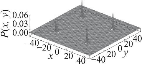
Figure 6: Probability distribution of zero-energy corner states with the potential $\theta_{x}(x)$ and $\theta_{y}(y)$ specified in the main text. We here plot one out of the totally eight corner states that are degenerate to a nearly zero eigenvalue. We set $\hbar=a=\Delta t=1$.

Note that each corner state is defined as localized at one of the four corners of the domain; the state represented in Fig. 6 is a superposition of the four corner states.

III Summary

To summarize, we proposed a new DTQW in multi-dimensional systems, whose continuum limit is the extended Dirac equation which can be further mapped to the Schrödinger equation. We successfully reproduced with our DTQW the dynamics similar to that of a Schrödinger particle under a harmonic potential. We also observed topological edge and corner states with discontinuous effective potentials in one- and two-dimensional systems simply by manipulating the coin operators of our DTQW. We thereby claim that the present DTQW is a powerful platform of numerical simulation and experimental implementation of the Dirac and Schrödinger particles.

As a final remark, increasing $\theta_{y}$ further from the case in Fig. 2(b), we find the spectrum in Fig. 7. We have numerically confirmed that the states enclosed in the openings of the bulk bands are edge states; see Appendix LABEL:appendmomotaro of the bulk band structure. This implies that our DTQW accommodates a further symmetry that protects these enclosed edge states, but we have not resolved yet what symmetry it is.

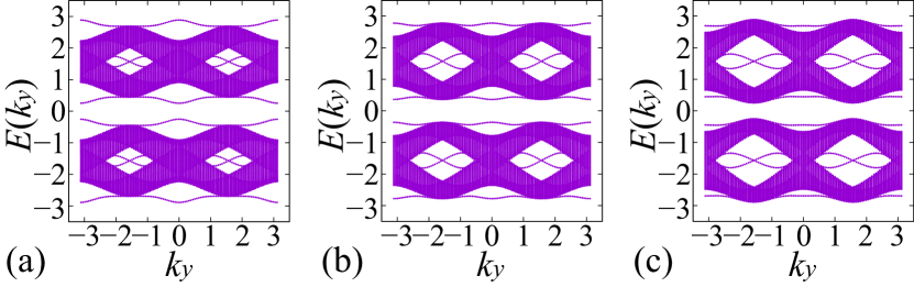
Figure 7: Dispersion relation of the quasi-energy spectra $E(k_{y})$ for the domain-wall structure in $\theta_{x}(x)$ as specified in the main text with (a) $\theta_{y}=\pi/6$, (b) $\theta_{y}=\pi/4$ and (c) $\theta_{y}=\pi/3$. We set $\hbar=a=\Delta t=1$.

Appendix A Eigenvalues of the 2D extended Dirac Hamiltonian

In the present Appendix, we describe how to obtain the eigenvalues and eigenvectors of our 2D extended Dirac Hamiltonian (I) out of those of the 1D Dirac Hamiltonian (6). The former should give the quasi-energy eigenvalues and eigenvectors of our 2D DTQW within the Trotter approximation, particularly near zero energy, that is, near the eigenvalue unity of the time-evolution operator.

We first introduce the general formalism in App. A.1. We then present the explicit solutions in the case of linear mass terms in App. A.2 and in the case of stepwise mass terms in App. LABEL:appendtopo.

A.1 General formalism

We first set the eigenstates of $H_{\mathrm{D}_{x}}$ $H_{\mathrm{D}_{y}}$ as in

$$H_{\mathrm{D}_{x}}\ket*{\psi^{\mathrm{D},(1)}_{E_{x}}} =E_{x}\ket*{\psi^{\mathrm{D},(1)}_{E_{x}}},$$ (30)

$$H_{\mathrm{D}_{y}}\ket*{\psi^{\mathrm{D},(1)}_{E_{y}}} =E_{y}\ket*{\psi^{\mathrm{D},(1)}_{E_{y}}}$$ (31)

with the normalization

$$\innerproduct*{\psi^{\mathrm{D},(1)}_{E_{x}}}{\psi^{\mathrm{D},(1)}_{E_{x}}}=\innerproduct*{\psi^{\mathrm{D},(1)}_{E_{y}}}{\psi^{\mathrm{D},(1)}_{E_{y}}}=1.$$ (32)

For a shorthand, let their direct product denoted by

$$\ket{\psi^{\mathrm{D},(1)}_{Ex,E_{y}}}:=\ket*{\psi^{\mathrm{D},(1)}_{E_{x}}}\ket*{\psi^{\mathrm{D},(1)}_{E_{y}}}.$$ (33)

We now assume the Ansatz for the eigenstate of our 2D extended Dirac Hamiltonian

$$H_{\mathrm{D}}^{(2)}:=H_{\mathrm{D}_{x}}\otimes\tau^{0}+\sigma^{x}\otimes H_{\mathrm{D}_{y}}$$ (34)

of the form

$$\ket{\psi^{\mathrm{D},(2)}_{E}}=\quantity(\gamma+\delta\sigma^{x})\ket{\psi^{\mathrm{D},(1)}_{Ex,E_{y}}},$$ (35)

where $\gamma$ and $\delta$ are real coefficients to be determined hereafter. From the eigenvalue equation

$$H_{\mathrm{D}}^{(2)}\ket{\psi^{\mathrm{D},(2)}_{E}}=E\ket{\psi^{\mathrm{D},(2)}_{E}},$$ (36)

we obtain

$$\quantity[\gamma\quantity(E_{x}+E_{y}\sigma^{x})+\delta\quantity(-E_{x}\sigma^{x}+E_{y})]\ket{\psi^{\mathrm{D},(1)}_{Ex,E_{y}}}$$

$$\qquad=E\quantity(\gamma+\delta\sigma^{x})\ket{\psi^{\mathrm{D},(1)}_{Ex,E_{y}}},$$ (37)

where we used the anti-commutation relation

$$\anticommutator{H_{\mathrm{D}_{x}}}{\sigma^{x}}=\anticommutator{\quantity(\epsilon\sigma^{z}p_{x}+m_{x}(x)\sigma^{y})}{\sigma^{x}}=0.$$ (38)

We thereby find the equations for the coefficients as

$$\gamma E_{x}+\delta E_{y} =\gamma E,$$ (39)

$$\gamma E_{y}-\delta E_{x} =\delta E.$$ (40)

First, let us eliminate $E$ from the set of the equations. We then find

$$2\gamma\delta E_{x}=\quantity(\gamma^{2}-\delta^{2})E_{y},$$ (41)

which motivates us to define the transformation of the coefficients of the forms

$$\gamma=A\cos\phi,\quad\delta=A\sin\phi.$$ (42)

We then have from Eq. (41)

$$\tan 2\phi=\frac{E_{y}}{E_{x}},$$ (43)

which determines the phase coefficient $\phi$ for the specific solutions of Eqs. (30) and (31). The amplitude coefficient $A$, on the other hand, is found from the normalization

$$1 =\innerproduct{\psi^{\mathrm{D},(2)}_{E}}{\psi^{\mathrm{D},(2)}_{E}}=\gamma^{2}+\delta^{2}+2\gamma\delta s$$

$$=A^{2}(1+s\sin 2\phi),$$ (44)

where $s:=\expectationvalue{\sigma^{x}}{\psi^{\mathrm{D},(1)}_{E_{x}}}$. We let $A$ undetermined in the present Appendix since it depends on the specific form of the eigenstate $\ket{\psi^{\mathrm{D},(1)}_{E_{x}}}$.

The set of equations (39) and (40) further produces

$$E_{x}=E\cos 2\phi,\qquad E_{y}=E\sin 2\phi,$$ (45)

and hence

$$E=\pm\sqrt{{E_{x}}^{2}+{E_{y}}^{2}}.$$ (46)

This implies that our 2D extended Dirac Hamiltonian (I) is indeed a precise direct product of independent components of 1D Dirac Hamiltonians $H_{\mathrm{D}_{x}}$ and $H_{\mathrm{D}y}$, and further implies that the 2D DTQW presented in Sec. II is also a precise direct product of independent components of 1D DTQW in the $x$ and $y$ directions

From Eq. (46) we can conclude the following. First, the zero-energy eigenstate of $H_{\mathrm{D}}^{(2)}$, if any, can be constructed only from the zero-energy eigenstates of $H_{\mathrm{D}_{x}}$ and $H_{\mathrm{D}_{y}}$, which is indeed simply given by

$$\ket{\psi^{\mathrm{D},(2)}_{E=0}}=\ket{\psi^{\mathrm{D},(1)}_{E_{x}=0}}\ket{\psi^{\mathrm{D},(1)}_{E_{y}=0}}.$$ (47)

Second, if there is an energy gap in the spectrum of either of $H_{\mathrm{D}_{x}}$ or $H_{\mathrm{D}_{y}}$, then the spectrum of $H_{\mathrm{D}}^{(2)}$ has an energy gap.

A.2 Case of the linear potentials (13)

We here explicitly obtain the Gaussian form of the zero-energy eigenstate of the 2D extended Dirac Hamiltonian (I) under the linear potentials (13). The eigenstate of the eigenvalue unity of the time-evolution operator $U^{(2)}$, which state we used for the initial state of our simulation in Subsec. II.1, is given by the state given here within the Trotter approximation.

A.2.1 Eigenvalues of the 1D Dirac Hamiltonian (6)

Let us first derive eigenstates of the 1D Dirac Hamiltonian (6) with $m_{x}(x)=\beta x$. The Schrödinger Hamiltonian after the unitary transformation $V=\exp(\mathrm{i}\sigma^{y}\pi/4)$ reads (c) (d) (e) (f) Figure 9: Band structure for $\theta_{x}=\pi/3$ and $\theta_{y}=0$. (a) and (b) Energy bands from two different viewpoints. (c), (d) and (e) Cross sections of the bands at $k_{x}=0$, $k_{x}=\pi/2$ and $k_{x}=\pi$, respectively. (f) Projection of the bands over the $k_{x}$ axis onto the $k_{y}$ axis. We set $\hbar=a=\Delta t=1$. When projected on the $k_{y}$ axis, each of the upper and lower energy band appears to be filled.

For $\theta_{y}=\pi/3$, on the other hand, all bands are open on the lines $k_{x}=0,\pm\pi$ and $k_{y}=0,\pm\pi$ except for the Dirac points $(k_{x},k_{y})=(0,0),(\pm\pi/2,\pm\pi/2),(\pm\pi,\pm,\pi)$; see Fig. A.2.1.

(a)

(b)

(c)

(d)

(e)

(f)

Figure 10: Band structure for $\theta_{x}=\pi/3$ and $\theta_{y}=\pi/3$. (a) and (b) Energy bands from two different viewpoints. (c), (d) and (e) Cross sections of the bands at $k_{x}=0$, $k_{x}=\pi/2$ and $k_{x}=\pi$, respectively. (f) Projection of the bands over the $k_{x}$ axis onto the $k_{y}$ axis. We set $\hbar=a=\Delta t=1$.

When projected on the $k_{y}$ axis, we can now see large openings in each of the upper and lower bands. When we introduce the effective potential

$$\theta_{x}(x)=\begin{cases}-\pi/3&\quad\mbox{for $|x|>L_{x}/2$},\\ \pi/3&\quad\mbox{for $|x|\leq L_{x}/2$},\end{cases}$$ (86)

we see edge modes in the openings as in Fig. 7 of the main text.

Figure A.2.1 shows the variation of the cross sections on $k_{x}=0$, $k_{x}=\pi/2$ and $k_{x}=\pi$ for $\theta_{y}=0,\pi/12,\pi/6,\pi/4,\pi/3$.

(a)

(b)

(c)

(d)

(e)

(f)

(g)

(h)

(i)

(j)

(k)

(l)

(m)

(n)

(o)

Figure 11: Cross sections of the bands at $k_{x}=0$, $k_{x}=\pi/2$ and $k_{x}=\pi$ on the first, second and third columns, respectively. We vary $\theta_{y}$ to $0$, $\pi/12$, $\pi/6$, $\pi/4$ and $\pi/3$ on the five rows from top to bottom, respectively. We set $\hbar=a=\Delta t=1$.

We can see the openings at each cross section become wider as we increase $\theta_{y}$.

References

- Aharonov et al. (1993) Y. Aharonov, L. Davidovich, and N. Zagury, Phys. Rev. A 48, 1687 (1993).
- Meyer (1996) D. A. Meyer, Journal of Statistical Physics 85, 551 (1996).
- Feynman and Hibbs (1965) R. P. Feynman and A. R. Hibbs, Quantum mechanics and path integrals, International series in pure and applied physics (McGraw-Hill, New York, NY, 1965).
- Farhi and Gutmann (1998) E. Farhi and S. Gutmann, Phys. Rev. A 58, 915 (1998).
- Ambainis et al. (2001) A. Ambainis, E. Bach, A. Nayak, A. Vishwanath, and J. Watrous, in Proceedings of the Thirty-Third Annual ACM Symposium on Theory of Computing, STOC ’01 (Association for Computing Machinery, New York, NY, USA, 2001) pp. 37–49.
- Asaka et al. (2021) R. Asaka, K. Sakai, and R. Yahagi, Quantum Science and Technology 6, 035004 (2021).
- Engel et al. (2007) G. S. Engel, T. R. Calhoun, E. L. Read, T.-K. Ahn, T. Mančal, Y.-C. Cheng, R. E. Blankenship, and G. R. Fleming, Nature 446, 782 (2007).
- Dudhe et al. (2022) N. Dudhe, P. K. Sahoo, and C. Benjamin, Phys. Chem. Chem. Phys. 24, 2601 (2022).
- Oka et al. (2005) T. Oka, N. Konno, R. Arita, and H. Aoki, Phys. Rev. Lett. 94, 100602 (2005).
- Kitagawa et al. (2010) T. Kitagawa, M. S. Rudner, E. Berg, and E. Demler, Phys. Rev. A 82, 033429 (2010).
- Kitagawa (2012) T. Kitagawa, Quantum Information Processing 11, 1107 (2012).
- Asbóth and Obuse (2013) J. K. Asbóth and H. Obuse, Phys. Rev. B 88, 121406 (2013).
- Strauch (2006) F. W. Strauch, Phys. Rev. A 73, 054302 (2006).
- Di Franco et al. (2011) C. Di Franco, M. Mc Gettrick, and T. Busch, Phys. Rev. Lett. 106, 080502 (2011).
- Bru et al. (2016) L. A. Bru, G. J. de Valcárcel, G. Di Molfetta, A. Pérez, E. Roldán, and F. Silva, Phys. Rev. A 94, 032328 (2016).
- Arrighi et al. (2018) P. Arrighi, G. Di Molfetta, I. Márquez-Martín, and A. Pérez, Phys. Rev. A 97, 062111 (2018).
- Murani et al. (2017) A. Murani, A. Kasumov, S. Sengupta, Y. A. Kasumov, V. T. Volkov, I. I. Khodos, F. Brisset, R. Delagrange, A. Chepelianskii, R. Deblock, H. Bouchiat, and S. Guéron, Nature Communications 8, 15941 (2017).
- Imhof et al. (2018) S. Imhof, C. Berger, F. Bayer, J. Brehm, L. W. Molenkamp, T. Kiessling, F. Schindler, C. H. Lee, M. Greiter, T. Neupert, and R. Thomale, Nature Physics 14, 925 (2018).
- Peterson et al. (2018) C. W. Peterson, W. A. Benalcazar, T. L. Hughes, and G. Bahl, Nature 555, 346 (2018).
- Ryder (1996) L. H. Ryder, Quantum Field Theory, 2nd ed. (Cambridge University Press, 1996).
- Benalcazar et al. (2017a) W. A. Benalcazar, B. A. Bernevig, and T. L. Hughes, Science 357, 61 (2017a), http://science.sciencemag.org/content/357/6346/61.full.pdf .
- Hayashi (2018) S. Hayashi, Communications in Mathematical Physics 364, 343 (2018).
- Schindler et al. (2017) F. Schindler, A. M. Cook, M. G. Vergniory, Z. Wang, S. S. P. Parkin, B. A. Bernevig, and T. Neupert, ArXiv e-prints (2017), arXiv:1708.03636 [cond-mat.mes-hall] .
- Langbehn et al. (2017) J. Langbehn, Y. Peng, L. Trifunovic, F. von Oppen, and P. W. Brouwer, Phys. Rev. Lett. 119, 246401 (2017).
- Song et al. (2017) Z. Song, Z. Fang, and C. Fang, Phys. Rev. Lett. 119, 246402 (2017).
- Benalcazar et al. (2017b) W. A. Benalcazar, B. A. Bernevig, and T. L. Hughes, Phys. Rev. B 96, 245115 (2017b).
- Jackiw and Rebbi (1976) R. Jackiw and C. Rebbi, Phys. Rev. D 13, 3398 (1976).
- Shenvi et al. (2003) N. Shenvi, J. Kempe, and K. B. Whaley, Phys. Rev. A 67, 052307 (2003).
- Yamagishi et al. (2023) M. Yamagishi, N. Hatano, and O. Hideaki, “Defining a quantum active particle using non-Hermitian quantum walk (unpublished),” (2023).
- Schweitzer et al. (1998) F. Schweitzer, W. Ebeling, and B. Tilch, Phys. Rev. Lett. 80, 5044 (1998).
- Shen (2013) S.-Q. Shen, Topological insulators, 2013th ed., Springer Series in Solid-State Sciences (Springer, Berlin, Germany, 2013).
- Kitaev (2009) A. Kitaev, AIP Conference Proceedings 1134, 22 (2009), https://aip.scitation.org/doi/pdf/10.1063/1.3149495 .
- Ryu et al. (2010) S. Ryu, A. P. Schnyder, A. Furusaki, and A. W. W. Ludwig, New Journal of Physics 12, 065010 (2010).
- Yoshimura et al. (2023) Y. Yoshimura, S. Hayashi, K.-I. Imura, and T. Nakanishi, “Bulk-edge-corner correspondence at an arbitrary angle (unpublished),” (2023).