Quantum ensembles and the statistical operator: a tutorial

Abstract

The main purpose of this tutorial is to elucidate in details what should be meant by ensemble of states in quantum mechanics, and to properly address the problem of discriminating, exactly or approximately, two different ensembles. To this aim we review the notion and the definition of quantum ensemble as well as its relationships with the concept of statistical operator in quantum mechanics. We point out the implicit assumptions contained in introducing a correspondence between quantum ensembles and the corresponding single-particle statistical operator, and discuss some issues arising when these assumptions are not satisfied. We review some subtleties leading to apparent paradoxes, and illustrate the role of approximate quantum cloning. In particular, we review some examples of practical interest where different (but equivalent) preparations of a quantum system, i.e. different ensembles corresponding to the same single-particle statistical operator, may be successfully discriminated exploiting multiparticle correlations, or some a priori knowledge about the number of particles in the ensemble.

1 Introduction

As matter of fact, fundamental postulates of quantum mechanics do not allow to discriminate two ensembles corresponding the same statistical (density) operator. Approximate discrimination is also forbidden by fundamental laws of physics, since it would violate the no-signaling condition imposed by causality. Despite this facts, one may find some claims in the literature about the possible discrimination of ensembles corresponding to the same density operator. In particular, specific schemes have been put forward [1, 2, 3, 4], involving finite set of particles sampled from a given ensemble, or ensembles prepared with inner correlations.

The main goal of this tutorial is to remove the apparent paradoxes by addressing in details what should be meant by ensemble of states in quantum mechanics, and to address properly the problem of discriminating, exactly or approximately, two different ensembles. To this purpose, we review the notion and the definition of quantum ensemble as well as its relationships with the concept of statistical operator in quantum mechanics. We point out the implicit assumptions contained in introducing a correspondence between quantum ensembles and the corresponding single-particle statistical operator, and review the apparent paradoxes arising when these assumptions are not satisfied.

As we will see, the paradoxes arise from mixing up the two different concepts of single-particle and many-particles statistical operators or to assume a fixed number of particle in the ensembles [5, 6, 7]. A detailed analysis of the measurement schemes mentioned above shows that discrimination is indeed possible, but also that the involved ensembles correspond to the same single-particle density operator but different many-particles ones. In other words, there are no paradoxes unless the measurement schemes are analyzed in naive way.

The tutorial is structured as follows. In the next Section we review the definition of ensemble and statistical operator in quantum mechanics, also emphasizing the implicit assumptions needed to establish a correspondence between quantum ensembles and the corresponding single-particle statistical operator. In Section 3 we briefly discuss the connection between the no-cloning theorem and the impossibility of discriminating ensembles with the same density operator and show that also approximate approximate quantum cloning machines (AQCM) cannot be used for this task. In Section 4 we discuss some measurement schemes where discrimination of seemingly equivalent ensembles is realized and show that this situation arise when the implicit assumptions contained in introducing a correspondence between quantum ensembles and the corresponding single-particle statistical operator, are not satisfied. Section 5 closes the tutorial with some concluding remarks.

2 The statistical operator of a quantum system

According to the basic postulates of quantum mechanics, the states of a physical system are described by normalized vectors $|\psi\rangle$, $\langle\psi|\psi\rangle=1$, of a Hilbert space $H$. Composite systems, either made by more than one physical object or by the different degrees of freedom of the same entity, are described by tensor product $H_{1}\otimes H_{2}\otimes...$ of the corresponding Hilbert spaces and the overall state of the system is a vector in the global space. As far as the Hilbert space description of physical systems is adopted then we have the superposition principle, which says that if $|\psi_{1}\rangle$ and $|\psi_{2}\rangle$ are possible states of a system, then also any (normalized) linear combination $\alpha|\psi_{1}\rangle+\beta|\psi_{2}\rangle$, $\alpha,\beta\in{\mathbbm{C}}$, $|\alpha|^{2}+|\beta|^{2}=1$ of the two states is an admissible state of the system.

Observable quantities are described by Hermitian operators $X$. Any Hermitian operator $X=X^{\dagger}$, admits a spectral decomposition $X=\sum_{x}xP_{x}$, in terms of its real eigenvalues $x$, which are the possible value of the observable, and of the projectors $P_{x}=|x\rangle\langle x|$, $P_{x},P_{x^{\prime}}=\delta_{xx^{\prime}}P_{x}$ on its eigenvectors $X|x\rangle=x|x\rangle$, which form a basis for the Hilbert space, i.e. a complete set of orthonormal states with the properties $\langle x|x^{\prime}\rangle=\delta_{xx^{\prime}}$ (orthonormality), and $\sum_{x}|x\rangle\langle x|=\mathbbm{I}$ (completeness, we omitted to indicate the dimension of the Hilbert space). $L(H)$ is the linear space of (linear) operators from $H$ to $H$, which itself is a Hilbert s pace with scalar product provided by the trace operation, i.e. upon denoting by $|A\rangle\rangle$ operators seen as elements of $L(H)$, we have $\langle\langle A|B\rangle\rangle=\hbox{Tr}[A^{\dagger}B]$.

The probability $p_{x}$ of obtaining the outcome $x$ from the measurement of the observable $X$ and the overall expectation value $\langle X\rangle$ are given by

$$p_{x} =\left|\langle\psi|x\rangle\right|^{2}=\langle\psi|P_{x}|\psi\rangle=\sum_{n}\langle\psi|\varphi_{n}\rangle\langle\varphi_{n}|P_{x}|\psi\rangle$$

$$=\sum_{n}\langle\varphi_{n}|P_{x}|\psi\rangle\langle\psi|\varphi_{n}\rangle=\hbox{Tr}\left[|\psi\rangle\langle\psi|\,P_{x}\right]$$ (1)

and $\langle X\rangle=\langle\psi|X|\psi\rangle=\hbox{Tr}\left[|\psi\rangle\langle\psi|\,X\right]$. This is the Born rule and it is the fundamental recipe to connect the mathematical description of a quantum state to the prediction of quantum theory on the results of an experiment. The state of the system after the measurement is the projection of the state before the measurement on the eigenspace of the observed eigenvalue, i.e.

$$|\psi_{x}\rangle=\frac{1}{\sqrt{p_{x}}}\,P_{x}|\psi\rangle$$

Let us nos suppose to deal with a quantum system whose preparation is not completely under control. What we know is that the system is prepared in the state $|\psi_{k}\rangle$ with probability $p_{k}$, i.e. that the system is described by the statistical ensemble $\{p_{k},|\psi_{k}\rangle\}$, $\sum_{k}p_{k}=1$, where the states $\{|\psi_{k}\rangle\}$ are not, in general, orthogonal. The expected value of an observable $X$ may be evaluated as follows

$$\langle X\rangle =\sum_{k}p_{k}\langle X\rangle_{k}=\sum_{k}p_{k}\langle\psi_{k}|X|\psi_{k}\rangle=\sum_{n\,p\,k}p_{k}\langle\psi_{k}|\varphi_{n}\rangle\langle\varphi_{n}|X|\varphi_{p}\rangle\langle\varphi_{p}|\psi_{k}\rangle$$

$$=\sum_{n\,p\,k}p_{k}\langle\varphi_{p}|\psi_{k}\rangle\langle\psi_{k}|\varphi_{n}\rangle\langle\varphi_{n}|X|\varphi_{p}\rangle=\sum_{n\,p}\langle\varphi_{p}|\varrho|\varphi_{n}\rangle\langle\varphi_{n}|X|\varphi_{p}\rangle$$

$$=\sum_{p}\langle\varphi_{p}|\varrho\,X|\varphi_{p}\rangle=\hbox{Tr}\left[\varrho\,X\right]\,$$

where

$$\varrho=\sum_{k}p_{k}\,|\psi_{k}\rangle\langle\psi_{k}|$$

is the statistical (density) operator of the system under investigation. The $|\varphi_{n}\rangle$’s in the above formula are a basis for the Hilbert space and we used the trick of suitably inserting two resolutions of the identity $\mathbbm{I}=\sum_{n}|\varphi_{n}\rangle\langle\varphi_{n}|$. The formula is of course trivial if the $|\psi_{k}\rangle$’s are themselves a basis or a subset of a basis.

Theorem 2.1

An operator $\varrho$ is the density operator associated to an ensemble $\{p_{k},|\psi_{k}\rangle\}$ is and only if it is a positive (hence selfadjoint) operator with unit trace $\hbox{Tr}\left[\varrho\right]=1$.

Proof 2.2.

If $\varrho=\sum_{k}p_{k}|\psi_{k}\rangle\langle\psi_{k}|$ is a density operator then $\hbox{Tr}[\varrho]=\sum_{k}p_{k}=1$ and for any vector $|\varphi\rangle\in H$, $\langle\varphi|\varrho|\varphi\rangle=\sum_{k}p_{k}|\langle\varphi|\psi_{k}\rangle|^{2}\geq 0$. Viceversa, if $\varrho$ is a positive operator with unit trace than it can be diagonalized and the sum of eigenvalues is equal to one. Thus it can be naturally associated to an ensemble.

As it is true for any operator, the density operator may be expressed in terms of its matrix elements in a given basis, i.e. $\varrho=\sum_{np}\varrho_{np}|\varphi_{n}\rangle\langle\varphi_{p}|$ where $\varrho_{np}=\langle\varphi_{n}|\varrho|\varphi_{p}\rangle$ is usually referred to as the density matrix of the system. Of course, the density matrix of a state is diagonal if we use a basis which coincides or includes the set of eigenvectors of the density operator, whereas it contains off-diagonal elements otherwise.

Different ensembles may lead to the same density operator. In this case they have the same expectation values for any operator and thus are physically indistinguishable. In other words, different preparations of ensembles leading to the same density operator are actually the same state, i.e. the density operator appears to provide the natural and fundamental quantum description of physical systems [8, 9].

How this reconciles with the above postulate saying ”physical systems are described by vectors in a Hilbert space”?

In order to see how it works let us first notice that according to the postulates above the action of ”measuring nothing” should be described by the identity operator $\mathbbm{I}$. Indeed the identity is Hermitian and has the single eigenvalues $1$, corresponding to the persistent result of measuring nothing. Besides, the eigenprojector corresponding to the eigenvalue $1$ is the projector over the whole Hilbert space and thus we have the consistent prediction that the state after the ”measurement” is left unchanged. Let us consider a situation in which a bipartite system prepared in the state $|\psi_{\scriptscriptstyle AB}\rangle\rangle\in H_{{\scriptscriptstyle A}}\otimes H_{{\scriptscriptstyle B}}$ is subjected to the measurement of an observable $X=\sum_{x}P_{x}\in L(H_{\scriptscriptstyle A})$, $P_{x}=|x\rangle\langle x|$ i.e. a measurement involving only the degree of freedom described by the Hilbert space $H_{\scriptscriptstyle A}$. The overall observable measured on the system is thus $\boldsymbol{X}=X\otimes\mathbbm{I}_{\scriptscriptstyle B}$, with spectral decomposition $\boldsymbol{X}=\sum_{x}x\,\boldsymbol{Q}_{x}$, $\boldsymbol{Q}_{x}=P_{x}\otimes\mathbbm{I}_{\scriptscriptstyle B}$. The probability distribution of the outcomes is then obtained using the Born rule, i.e.

$$p_{x}=\hbox{Tr}_{\scriptscriptstyle AB}\Big{[}|\psi_{\scriptscriptstyle AB}\rangle\rangle\langle\langle\psi_{\scriptscriptstyle AB}|\,P_{x}\otimes\mathbbm{I}_{\scriptscriptstyle B}\Big{]}$$ (2)

On the other hand, since the measurement has been performed only on the system $A$ one expects the Born rule to be valid also at the level of single system and a question arises on the form of the object $\varrho_{\scriptscriptstyle A}$ which allows one to write $p_{x}=\hbox{Tr}_{\scriptscriptstyle A}\left[\varrho_{\scriptscriptstyle A}\,P_{x}\right]$ i.e. the Born rule as a trace only over the Hilbert space $H_{\scriptscriptstyle A}$. Upon inspecting Eq. (2), one sees that a suitable mapping $|\psi_{\scriptscriptstyle AB}\rangle\rangle\langle\langle\psi_{\scriptscriptstyle AB}|\rightarrow\varrho_{\scriptscriptstyle A}$ is provided by the partial trace $\varrho_{\scriptscriptstyle A}=\hbox{Tr}_{\scriptscriptstyle B}\left[|\psi_{\scriptscriptstyle AB}\rangle\rangle\langle\langle\psi_{\scriptscriptstyle AB}|\right]$. Indeed, for the operator $\varrho_{\scriptscriptstyle A}$ defined by the above partial trace we have $\hbox{Tr}_{\scriptscriptstyle A}[\varrho_{\scriptscriptstyle A}]=\hbox{Tr}_{\scriptscriptstyle AB}\left[|\psi_{\scriptscriptstyle AB}\rangle\rangle\langle\langle\psi_{\scriptscriptstyle AB}|\right]=1$ and, for any vector $|\varphi\rangle\in H_{\scriptscriptstyle A}$ , $\langle\varphi_{\scriptscriptstyle A}|\varrho_{\scriptscriptstyle A}|\varphi_{\scriptscriptstyle A}\rangle=\hbox{Tr}_{\scriptscriptstyle AB}\left[|\psi_{\scriptscriptstyle AB}\rangle\rangle\langle\langle\psi_{\scriptscriptstyle AB}|\,|\varphi_{\scriptscriptstyle A}\rangle\langle\varphi_{\scriptscriptstyle A}|\otimes\mathbbm{I}_{\scriptscriptstyle B}\right]\geq 0$. Being a positive, unit trace, operator $\varrho_{\scriptscriptstyle A}$ is itself a density operator according to the definition above. It should be also noticed that actually, the partial trace is the unique operation which allows to maintain the Born rule at both level i.e. the unique operation leading to the correct description of observable quantities for subsystems of a composite system. Let us state this as a theorem [10]:

Theorem 2.3.

The unique mapping $|\psi_{\scriptscriptstyle AB}\rangle\rangle\langle\langle\psi_{\scriptscriptstyle AB}|\rightarrow\varrho_{\scriptscriptstyle A}=f(\psi_{\scriptscriptstyle AB})$ from $H_{\scriptscriptstyle A}\otimes H_{\scriptscriptstyle B}$ to $H_{\scriptscriptstyle A}$ for which $\hbox{Tr}_{\scriptscriptstyle AB}\left[|\psi_{\scriptscriptstyle AB}\rangle\rangle\langle\langle\psi_{\scriptscriptstyle AB}|\,P_{x}\otimes\mathbbm{I}_{\scriptscriptstyle B}\right]=\hbox{Tr}_{\scriptscriptstyle A}\left[f(\psi_{\scriptscriptstyle AB})\,P_{x}\right]$ is the partial trace $f(\psi_{\scriptscriptstyle AB})\equiv\varrho_{\scriptscriptstyle A}=\hbox{Tr}_{\scriptscriptstyle B}\left[|\psi_{\scriptscriptstyle AB}\rangle\rangle\langle\langle\psi_{\scriptscriptstyle AB}|\right]$.

Proof 2.4.

Basically the proof reduces to the fact that the set of operators on $H_{\scriptscriptstyle A}$ is itself a Hilbert space $L(H_{\scriptscriptstyle A})$ with scalar product given by $\langle\langle A|B\rangle\rangle=\hbox{Tr}[A^{\dagger}B]$. Indeed, let us consider a basis of operators $\{M_{k}\}$ for $L(H_{\scriptscriptstyle A})$ and expand $f(\psi_{\scriptscriptstyle AB})=\sum_{k}M_{k}\hbox{Tr}_{\scriptscriptstyle A}[M_{k}^{\dagger}f(\psi_{\scriptscriptstyle AB})]$. Since $f$ is the map to preserve the Born rule we have

$$f(\psi_{\scriptscriptstyle AB})=\sum_{k}M_{k}\hbox{Tr}_{\scriptscriptstyle A}[M_{k}^{\dagger}\,f(\psi_{\scriptscriptstyle AB})]=\sum_{k}M_{k}\hbox{Tr}_{\scriptscriptstyle AB}\left[M_{k}^{\dagger}\otimes\mathbbm{I}_{\scriptscriptstyle B}\,|\psi_{\scriptscriptstyle AB}\rangle\rangle\langle\langle\psi_{\scriptscriptstyle AB}|\right]\,$$

and the thesis follows from the fact that in a Hilbert space the decomposition on a basis is unique.

The above result can be easily generalized to the case of a system which is initially described by a density operator $\varrho_{\scriptscriptstyle AB}$ and thus we conclude that when we focus attention to a subsystem of a composite larger system the unique mathematical description of ignoring part of the degrees of freedom is provided by the partial trace. It remains to be proved that the partial trace of a density operator is a density operator too. This is a very consequence of the definition that we put in form a little theorem.

Theorem 2.5.

The partial traces $\varrho_{\scriptscriptstyle A}=\hbox{Tr}_{\scriptscriptstyle B}[\varrho_{\scriptscriptstyle AB}]$, $\varrho_{\scriptscriptstyle B}=\hbox{Tr}_{\scriptscriptstyle A}[\varrho_{\scriptscriptstyle AB}]$ of the density operator of a bipartite system are themselves density operators for the reduced systems.

Proof 2.6.

We have $\hbox{Tr}_{\scriptscriptstyle A}[\varrho_{\scriptscriptstyle A}]=\hbox{Tr}_{\scriptscriptstyle B}[\varrho_{\scriptscriptstyle B}]=\hbox{Tr}_{\scriptscriptstyle AB}[\varrho_{\scriptscriptstyle AB}]=1$ and, for any state $|\varphi_{\scriptscriptstyle A}\rangle\in H_{\scriptscriptstyle A}$, $|\varphi_{\scriptscriptstyle B}\rangle\in H_{\scriptscriptstyle B}$,

$$\langle\varphi_{\scriptscriptstyle A}|\varrho_{\scriptscriptstyle A}|\varphi_{\scriptscriptstyle A}\rangle =\hbox{Tr}_{\scriptscriptstyle AB}\left[\varrho_{\scriptscriptstyle AB}\,|\varphi_{\scriptscriptstyle A}\rangle\langle\varphi_{\scriptscriptstyle A}|\otimes\mathbbm{I}_{\scriptscriptstyle B}\right]\geq 0$$

$$\langle\varphi_{\scriptscriptstyle B}|\varrho_{\scriptscriptstyle B}|\varphi_{\scriptscriptstyle B}\rangle =\hbox{Tr}_{\scriptscriptstyle AB}\left[\varrho_{\scriptscriptstyle AB}\,\mathbbm{I}_{\scriptscriptstyle A}\otimes|\varphi_{\scriptscriptstyle B}\rangle\langle\varphi_{\scriptscriptstyle B}|\right]\geq 0\,,$$

which prove positivity of both $\varrho_{\scriptscriptstyle A}$ and $\varrho_{\scriptscriptstyle B}$.

It also follows that the state of the ”unmeasured” subsystem after the observation of a specific outcome may be obtained as a partial trace of the projection of the state before the measurement on the eigenspace of the observed eigenvalue, i.e.

$$\varrho_{{\scriptscriptstyle B}x}=\frac{1}{p_{x}}\hbox{Tr}_{\scriptscriptstyle A}\left[P_{x}\otimes\mathbbm{I}_{\scriptscriptstyle B}\,\varrho_{\scriptscriptstyle AB}\,P_{x}\otimes\mathbbm{I}_{\scriptscriptstyle B}\right]=\frac{1}{p_{x}}\hbox{Tr}_{\scriptscriptstyle A}\left[\varrho_{\scriptscriptstyle AB}\,P_{x}\otimes\mathbbm{I}_{\scriptscriptstyle B}\right]\,$$

where, to write the second equality, we made use of the circularity of the trace and of the fact that we are in presence of a factorized projector. This is also referred to as the ”conditional state” of system $B$ after the observation of the outcome $x$ from a measurement of the observable $X$ performed on the system $A$.

2.1 Discussion

In several textbooks a distinction is made between ensembles coming from the ignorance about the preparation of a system and those emerging from measurements performed on bipartite systems. They are usually referred to as ensembles of the proper and improper kind respectively [11]. Actually, as it emerges clearly from the derivation reported above, there is no fundamental difference between the two kinds of ensembles and this classification is somehow artificial (though it has been useful in the development of the field).

The emerging definition is the following: a quantum ensemble is a collection of repeated identical preparations of the system, randomly generated according to a given probability distribution. When this definition is applicable then we have the fundamental result reported above: two ensembles corresponding to the same statistical operator cannot be discriminated by any kind of measurement, i.e. they are physically indistinguishable and do not correspond to different physical entities [12].

We want to emphasize, however, that the above definition contains two implicit assumptions that may not be verified in all the physical situation of interest. They are: i) the preparations are identical and random, i.e. no correlations are present within the ensemble, e.g. between subsequent preparations; ii) the number of preparations is not known or fixed: strictly speaking statistical operators describe ensembles made of infinite preparations, though this should be intended as large enough for the advent of the law of large numbers. Whenever the two conditions are not fulfilled the correspondence between ensembles and (single-particle) statistical operators is no longer ensured and (apparent) paradoxical situations may arises.

3 Quantum cloning and discrimination of ensembles

Before addressing the issues arising when the above assumptions are not satisfied, we briefly review and discuss the connections between i) the impossibility of discriminating ensembles with the same density operator and ii) the impossibility of perfectly replicating quantum information, i.e. the so-called no-cloning theorem. We also show that even approximate discrimination is not possible since this would violate the no-signaling condition imposed by causality. Quite obviously, feasible (approximate) quantum cloning machines, which have been designed to fulfill this condition, cannot be employed as well for discriminating ensembles [13, 14, 15].

Let us start by reviewing the no-cloning theorem in its general form

Theorem 3.1.

There is no unitary operation $U$ on $H_{\scriptscriptstyle A}\otimes H_{\scriptscriptstyle B}\otimes H_{\scriptscriptstyle C}$ that for given $|\omega\rangle_{\scriptscriptstyle B}$ and $|A\rangle_{\scriptscriptstyle C}$ is able to implement the transformation $U|\psi\rangle_{\scriptscriptstyle A}\otimes|\omega\rangle_{\scriptscriptstyle B}\otimes|A\rangle_{\scriptscriptstyle C}=|\psi\rangle_{\scriptscriptstyle A}\otimes|\psi\rangle_{\scriptscriptstyle B}\otimes|A_{\psi}\rangle_{\scriptscriptstyle C}$ for any $|\psi\rangle_{\scriptscriptstyle A}$.

From the operational point of view the theorem says that no physical device (initially prepared in the state $|A\rangle\in H_{\scriptscriptstyle C}$) may obtain two copies of a generic quantum state $|\psi\rangle_{\scriptscriptstyle A}$ starting from a single copy and by coupling the system under investigation to an ancillary system $B$ of the same dimension.

Proof 3.2.

The proof is based on the sole request of linearity of quantum mechanics. In fact if we require the device to work for a pair of states $|\varphi_{0}\rangle$ and $|\varphi_{1}\rangle$, i.e

$$U\,|\varphi_{0}\rangle_{\scriptscriptstyle A}\otimes|\omega\rangle_{\scriptscriptstyle B}\otimes|A\rangle_{\scriptscriptstyle C} =|\varphi_{0}\rangle_{\scriptscriptstyle A}\otimes|\varphi_{0}\rangle_{\scriptscriptstyle B}\otimes|A_{0}\rangle_{\scriptscriptstyle C}$$

$$U\,|\varphi_{1}\rangle_{\scriptscriptstyle A}\otimes|\omega\rangle_{\scriptscriptstyle B}\otimes|A\rangle_{\scriptscriptstyle C} =|\varphi_{1}\rangle_{\scriptscriptstyle A}\otimes|\varphi_{1}\rangle_{\scriptscriptstyle B}\otimes|A_{1}\rangle_{\scriptscriptstyle C}\,,$$

then, by linearity, one has

$$U\,\left(|\varphi_{0}\rangle_{\scriptscriptstyle A}+|\varphi_{1}\rangle_{\scriptscriptstyle A}\right)\otimes|\omega\rangle_{\scriptscriptstyle B}\otimes|A\rangle_{\scriptscriptstyle C}=|\varphi_{0}\rangle_{\scriptscriptstyle A}\otimes|\varphi_{0}\rangle_{\scriptscriptstyle B}\otimes|A_{0}\rangle_{\scriptscriptstyle C}+|\varphi_{1}\rangle_{\scriptscriptstyle A}\otimes|\varphi_{1}\rangle_{\scriptscriptstyle B}\otimes|A_{1}\rangle_{\scriptscriptstyle C}\,,$$

which is not what we are expecting from a cloning device, since the cloning of a superposition should correspond to

$$U\,\frac{1}{\sqrt{2}}\left(|\varphi_{0}\rangle_{\scriptscriptstyle A}+|\varphi_{1}\rangle_{\scriptscriptstyle A}\right)\otimes|\omega\rangle_{\scriptscriptstyle B}\otimes|A\rangle_{\scriptscriptstyle C}=\frac{1}{\sqrt{2}}\left(|\varphi_{0}\rangle_{\scriptscriptstyle A}+|\varphi_{1}\rangle_{\scriptscriptstyle A}\right)\otimes\frac{1}{\sqrt{2}}\left(|\varphi_{0}\rangle_{\scriptscriptstyle B}+|\varphi_{1}\rangle_{\scriptscriptstyle B}\right)\otimes|A_{01}\rangle_{\scriptscriptstyle C}\,.$$

In other words, linearity of quantum mechanics forbids the existence of a cloning machine for any unitary on $H_{\scriptscriptstyle A}\otimes H_{\scriptscriptstyle B}\otimes H_{\scriptscriptstyle C}$, i.e. any map on $H_{\scriptscriptstyle A}\otimes H_{\scriptscriptstyle B}$.

Figure 1: Schematic diagram of a hypothetical cloning device including the degrees of freedom of the apparatus. Linearity of quantum mechanics forbids the existence of this kind of device.

It is well known from the discussion about Bell’s inequalities that quantum nonlocality cannot be used to implement any kind of superluminal communication and, in turn, to violate causality (no-signaling condition), even in conjunction with the reduction postulate [15]. Let us now give some more details in order to connect this fact with the impossibility of quantum cloning and of discrimination of ensembles corresponding to the same statistical operator. Indeed, it is known as the no-cloning theorem was triggered as a response to a (wrong) proposal for superluminal communication named FLASH (first light amplification superluminal hookup) put forward by N. Herbert in 1982 [16].

The argument goes as follows: Let us assume that Alice and Bob share an entangled state of the form $|\psi\rangle\rangle=\frac{1}{\sqrt{2}}\left(|00\rangle\rangle+|11\rangle\rangle\right)$, where $|jj\rangle\rangle=|j\rangle\otimes|j\rangle$ and we employ the standard basis made of eigenstates of $\sigma_{3}$ in both Hilbert spaces. If Alice performs a measurement of the spin in a generic direction $\sigma_{\phi}$ she may obtain one of the two possible outcomes $\pm 1$ with equal probability $p=\frac{1}{2}$ and, correspondingly, Bob’s state is projected onto one of the two possible conditional states $|0\rangle_{\phi}=\cos\phi|0\rangle+\sin\phi|1\rangle$ and $|1\rangle_{\phi}=\cos\phi|0\rangle+\sin\phi|1\rangle$. Of course, if Bob does not know the result of Alice’ measurement his conditional state is given by $\varrho^{(1)}_{\scriptscriptstyle B}=\frac{1}{2}\left(|0\rangle_{\phi\phi}\langle 0|+|1\rangle_{\phi\phi}\langle 1|\right)=\frac{1}{2}\mathbbm{I}$. Analogously, if Alice performs the measurement of $\sigma_{3}$, then the reduction occurs on the states $|0\rangle$ and $|1\rangle$ but, without the knowledge of Alice’s results, the overall conditional state of Bob is $\varrho^{(3)}_{\scriptscriptstyle B}=\frac{1}{2}\left(|0\rangle\langle 0|+|1\rangle\langle 1|\right)=\frac{1}{2}\mathbbm{I}$. Being $\varrho^{(3)}_{\scriptscriptstyle B}=\varrho^{(1)}_{\scriptscriptstyle B}$ the impossibility of discriminating the two ensembles is equivalent to the impossibility for Bob to infer which measurement has been performed by Alice, i.e. it is not possible to exploit nonlocal correlations of entangled states to transmit information. The same argument may be easily repeated for any choice of the pair of measurements performed by Alice. In order to make the two ensembles distinguishable, at least partially, Alice should send to Bob some piece of information about the results of her measurement, using some traditional communication channel, thus ”saving causality”.

Let us now assume that Bob has at disposal a perfect quantum cloning machine and use it, in a scheme like the right part of Fig. 2, whenever Alice performs a measurement. If Alice measures $\sigma_{\phi}$ then the state that Bob is inserting into the cloning machine is either $|0\rangle_{\phi}$ or $|1\rangle_{\phi}$ with probability $p=\frac{1}{2}$. The overall state at disposal of Bob, at the output of the cloning machine and without knowing the result of Alice’s measurements, is thus given by

$$R_{\scriptscriptstyle B}^{(\phi)}=\frac{1}{2}\left[|0\rangle_{\phi\phi}\langle 0|\otimes|0\rangle_{\phi\phi}\langle 0|+|1\rangle_{\phi\phi}\langle 1|\otimes|1\rangle_{\phi\phi}\langle 1|\right]\,.$$

If Alice measures $\sigma_{3}$ the line of reasoning is the same and the state at disposal of Bob is described by the operator

$$R_{\scriptscriptstyle B}^{(3)}=\frac{1}{2}\left[|0\rangle\langle 0|\otimes|0\rangle\langle 0|+|1\rangle\langle 1|\otimes|1\rangle\langle 1|\right]\,.$$

Since $R_{\scriptscriptstyle B}^{(\phi)}\neq R_{\scriptscriptstyle B}^{(3)}$ it would be possible for Bob to discriminate the two states and, in turn, to infer which measurement has been performed by Alice just by looking at his local state. However, this is a clear violation of the no-signaling condition and, in fact, the no-cloning appeared soon after as a rebuttal of the FLASH proposal. Or, to say the same in other words, a perfect cloning machine would turn ensembles corresponding to the same statistical operators into ensembles with different statistical operators, making them distinguishable [17].

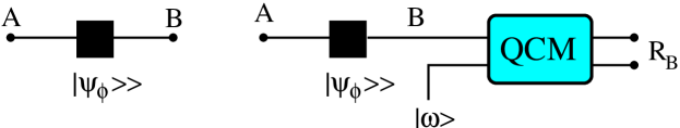
Figure 2: (Left): Alice and Bob share an entangled state. (Right): Schematic diagram of a hypothetical superluminal communication scheme exploiting a quantum cloning machine. The use of a cloning device would allow Bob to discriminate which measurement has been performed by Alice just by looking at his local state $R_{\scriptscriptstyle B}$.

3.1 Approximate cloning and discrimination of ensembles

As we have seen in the previous Section, the no-signaling condition forbids quantum cloning and, at the same time, both exact and approximate discrimination of ensembles with the same statistical operator. On the other hand, since approximate cloning machine fulfilling the no-signaling condition have been suggested, one may wonder whether this class of devices may permit approximate discrimination of ensembles corresponding to the same statistical operator. As we will see the answer is negative, thus showing the full equivalence of the no-signaling condition, the no-cloning theorem and the impossibility of discriminating ensembles with the same statistical operator.

Assuming the reader familiar with the impossibility of perfect quantum cloning from now on we will speak about ”quantum cloning machine”, (QCM) dropping the obvious specification ”approximate” (from time to time we will forget also the term ”quantum”). A generic $N\rightarrow M$ quantum cloning machine for pure states is a device involving a unitary operation, an ancillary system and an apparatus system, implementing a transformation of the form

$$|\psi\rangle^{\otimes N}\otimes|\omega\rangle^{\otimes(M-N)}\otimes|A\rangle_{\scriptscriptstyle C}\stackrel{{\scriptstyle U}}{{\longrightarrow}}|\Psi\rangle\,,$$

and for which the partial traces $\varrho_{j}={\rm Tr}\,_{\neq j}\big{[}|\Psi\rangle\langle\Psi|\big{]}$ possesses some similarity to the input state $|\psi\rangle$. In the above formulas $|\psi\rangle^{\otimes N}=|\psi\rangle\otimes...\otimes|\psi\rangle$ denotes the $N$-fold tensor product of the state $|\psi\rangle$ and ${\rm Tr}\,_{\neq j}[...]$ the partial trace over all the systems except the $j$-th one. In other words, one assumes to start with $N$ quantum system identically prepared in the state $|\psi\rangle$ and aims to end up with $M$ quantum systems prepared in some states $\varrho_{j}$, $j=1,...,M$, each being as close as possible to $|\psi\rangle$ according to some figure of merit quantifying the similarity between a pair of quantum states.

The standard figure of merit, employed to assess the performances of a cloning machine is the so-called single-clone fidelity, i.e. $F_{j}=\langle\psi|\varrho_{j}|\psi\rangle$. A quantum cloning machine is said universal: if the fidelities $F_{j}$ do not depend on the input state $|\psi\rangle$, and symmetric: if $F_{j}=F$, $\forall j$. A suitable figure of merit to globally assess a cloning machine is then the average of single-clone fidelities, i.e. $\overline{F}=\frac{1}{M}\sum_{j}\int_{S}d\psi\,F_{j}(\psi)$, where summing over $j$ implements the average over the clones and the integral (being $d\psi$ a formal notation to denote a suitable parametrization for the signals) over the set $S$ of possible input signals. For symmetric QCM we may avoid the averaging over the clones, and for universal the one over the signals. A quantum cloning machine is said optimal: if the average fidelity is maximal, consistently with the constraints imposed by quantum mechanics. The proof that a given QCM is optimal may be obtained in conjunction with fundamental constraints. As for example an optimal QCM could be a device giving a fidelity which is the maximum possible without violating the no-signaling condition.

The so-called Buzek-Hillery $1\rightarrow 2$ optimal cloning machine for qubit is realized by a three-qubit unitary transformation, which acts on the signal basis as follows (we omit to explicitly indicate the tensor product)

$$|0\rangle_{\scriptscriptstyle A}|\omega\rangle_{\scriptscriptstyle B}|A\rangle_{\scriptscriptstyle C} \stackrel{{\scriptstyle U}}{{\longrightarrow}}\sqrt{\frac{2}{3}}\,|0\rangle_{\scriptscriptstyle A}|0\rangle_{\scriptscriptstyle B}|1\rangle_{\scriptscriptstyle C}-\sqrt{\frac{1}{3}}\,|\tfrac{\sigma_{1}}{\sqrt{2}}\rangle\rangle_{{\scriptscriptstyle AB}}|0\rangle_{\scriptscriptstyle C}$$

$$|1\rangle_{\scriptscriptstyle A}|\omega\rangle_{\scriptscriptstyle B}|A\rangle_{\scriptscriptstyle C} \stackrel{{\scriptstyle U}}{{\longrightarrow}}-\sqrt{\frac{2}{3}}\,|1\rangle_{\scriptscriptstyle A}|1\rangle_{\scriptscriptstyle B}|0\rangle_{\scriptscriptstyle C}+\sqrt{\frac{1}{3}}\,|\tfrac{\sigma_{1}}{\sqrt{2}}\rangle\rangle_{{\scriptscriptstyle AB}}|1\rangle_{\scriptscriptstyle C}\,.$$ (3)

Explicit unitaries may be written for any choice of $\omega=0,1$ and $A=0,1$. Using the above transformations it is straightforward to see that the generic qubit state evolves as

$$|\psi\rangle_{\scriptscriptstyle A}|\omega\rangle_{\scriptscriptstyle B}|A\rangle_{\scriptscriptstyle C}\stackrel{{\scriptstyle U}}{{\longrightarrow}}\sqrt{\frac{2}{3}}\,|\psi\rangle_{\scriptscriptstyle A}|\psi\rangle_{\scriptscriptstyle B}|\psi^{\scriptscriptstyle\perp}\rangle_{\scriptscriptstyle C}-\sqrt{\frac{1}{6}}\,\Big{[}|\psi\rangle_{\scriptscriptstyle A}|\psi^{\scriptscriptstyle\perp}\rangle_{\scriptscriptstyle B}+|\psi^{\scriptscriptstyle\perp}\rangle_{\scriptscriptstyle A}|\psi\rangle_{\scriptscriptstyle B}\Big{]}|\psi\rangle_{\scriptscriptstyle C}\,,$$

where $\langle\psi|\psi^{\scriptscriptstyle\perp}\rangle=0$. Upon taking the partial traces over the systes BC and AC respectively one arrives at the following (identical) expression for the density operator of the two clones

$$\varrho_{\scriptscriptstyle A}=\varrho_{\scriptscriptstyle B}=\frac{5}{6}|\psi\rangle\langle\psi|+\frac{1}{6}|\psi^{\scriptscriptstyle\perp}\rangle\langle\psi^{\scriptscriptstyle\perp}|\>,$$

which says that the Buzek-Hillery cloning device is symmetric and universal and that the fidelity is given by $F=\tfrac{5}{6}$.

Optimality of this QCM may be proved in connection with the no-signaling condition, i.e. by proving that a larger fidelity would allow superluminal communication. To this aim let us consider the Bloch sphere representation of the generic input state $|\psi\rangle\langle\psi|=\frac{1}{2}\left(\mathbbm{I}+\boldsymbol{r}\cdot\boldsymbol{\sigma}\right)$ and of the corresponding clones from a universal and symmetric QCM, i.e. $\varrho_{\scriptscriptstyle A}=\varrho_{\scriptscriptstyle B}=\frac{1}{2}\left(\mathbbm{I}+\boldsymbol{r}^{\prime}\cdot\boldsymbol{\sigma}\right)$. Since for qubits $F={\rm Tr}\,[|\psi\rangle\langle\psi|\,\varrho_{\scriptscriptstyle A}]=\frac{1}{2}(1+\boldsymbol{r}\cdot\boldsymbol{r}^{\prime})$ we may write $\boldsymbol{r}^{\prime}=\eta\boldsymbol{r}$ where we have introduced the so-called ”shrinking factor” $0\leq\eta\leq 1$, which accounts for the degradation of the clones. The fidelity rewrites as $F=\frac{1}{2}(1+\eta)$ and for the Buzek-Hillery QCM we have $\eta=\frac{2}{3}$. Is this the maximum possible values? The answer is positive as it may be proved by imposing the no-signaling condition to any scheme as the one in the right panel of Fig. 2 which employs a universal and symmetric QCM. The proof proceeds as follows: if Alice measures either $\sigma_{1}$ or $\sigma_{3}$ and Bob use a cloning machine on his conditional state the output states will be of the form $R_{1}=\frac{1}{2}(R_{1}^{1}+R_{1}^{0})$ and $R_{3}=\frac{1}{2}(R_{3}^{1}+R_{3}^{0})$. If we impose that the $R$’s should be compatible with being the output of a symmetric and universal QCM i.e. such that ${\rm Tr}\,_{\scriptscriptstyle A}[R]={\rm Tr}\,_{\scriptscriptstyle B}[R]=\frac{1}{2}(\mathbbm{I}+\eta\,\boldsymbol{r}\cdot\boldsymbol{\sigma})$ and the no-signallign condition, then we end up with the condition $\eta\leq\frac{2}{3}$. The very same threshold ensures that $R_{1}=R_{3}$, i.e. approximate cloning do not turn single-qubit ensembles corresponding to the same statistical operators into two-qubit distinguishable ensembles.

4 Discrimination of seemingly equivalent ensembles

In this section we review some measurement schemes where discrimination of seemingly equivalent ensembles is realized, thus leading to an apparent contradiction. As mentioned above, these seemingly paradoxical situation arise when the implicit assumptions contained in introducing a correspondence between quantum ensembles and the corresponding single-particle statistical operator, are not satisfied.

4.1 Single- and many-particle density operator

Let us consider a spin system made of $N$ particles prepared randomly way. The state of the system is thus described the statistical operator:

$$\rho_{N}=\frac{1}{2^{N}}\sum_{j_{1},\ldots,j_{N}}P_{j_{1}}\otimes\cdots\otimes P_{j_{N}}\equiv\frac{1}{2^{N}}\mathbb{I}_{2^{N}}$$ (4)

where $\mathbb{I}_{2^{N}}$ is the identity operator in the space of dimension $2^{N}$, $j_{k}=\pm 1$ $\forall k$ and $P_{j_{k}}$ are projectors onto the subspace describing the spin of the particle $j_{k}$, e.g. eigenvectors of the Hamiltonian describing the spin of the single particle. Complete randomness is equivalent to the fact that all projectors contribute with the same weight in the density matrix. Let us now consider the two following ensembles of N particles: the ensemble $E_{1}$contains particles with spin directed as $z-axis$ while $E_{2}$ contains particles with spin along $x-axis$. In formula

$$E_{1}: |1\rangle|0\rangle|0\rangle|0\rangle\cdots\;\;random$$ (5)

$$E_{2}: |\uparrow\rangle|\downarrow\rangle|\uparrow\rangle|\uparrow\rangle\cdots\;\;random\,.$$ (6)

The two ensembles are equivalent and correspond to the same density operator $\rho=\frac{1}{2^{N}}\mathbb{I}_{2^{N}}$. If we look at the same systems as a collection of preparations of states of $m$-particle with $m<N$ then the density operator describing the two systems is given by the partial trace of $\rho_{N}$, i.e. $\rho_{m}=\frac{\mathbb{I}_{2^{m}}}{2^{m}}$. In particular, for ensembles of states of single-particle we have $\rho_{1}=\frac{\mathbb{I}_{1}}{2}$ and thus it is not possible to discriminate the two ensembles neither by single-particle measurements, nor by collective ones.

Suppose now to prepare the ensemble of $N$ particles as follows: we prepare the first particle with spin up, the second in the state with spin down and so on, and we separate two successive preparations by a time $\tau$ in order to label each particle. We then consider the following two ensembles: $E_{3}$ made of particles with spin along $z-axis$, and $E_{4}$, with spin along the $x-axis$. Explicitly

$$E_{3}: |1\rangle_{0}|0\rangle_{\tau}|1\rangle_{2\tau}|0\rangle_{3\tau}\cdots\;\;random$$ (7)

$$E_{4}: |\uparrow\rangle_{0}|\downarrow\rangle_{\tau}|\uparrow\rangle_{2\tau}|\downarrow\rangle_{3\tau}\cdots\;\;random\,.$$ (8)

If we see these two ensembles as preparations of single-particle states, they are equivalent, and correspond to statistical operator $\frac{\mathbb{I}}{2}$. However, if we look at the two ensembles as describing preparations of many-particle states, then they can be discriminated by measuring some collective observable, e.g. $\Sigma_{z}=\sigma_{z}\otimes\mathbb{I}\otimes\cdots+\cdots+\mathbb{I}\otimes\cdots\otimes\sigma_{z}$. In the following, we show this explicitly two- and three-particle observables. Eventually, we will generalize for case of N-particles.

If we look at the two ensembles $E_{3}$ and $E_{4}$ as describing a two-particle system, we immediately realize that they correspond to different pure states: $|1\rangle_{t}|0\rangle_{t+\tau}$ and $|\uparrow\rangle_{t}|\downarrow\rangle_{t+\tau}$. The observable $\Sigma_{z}$ for two particles, in the canonical basis (eigenvectors of $\sigma_{z}$ and $\mathbb{I}$) corresponds to the matrix $\Sigma_{z}=\hbox{Diag}(2,0,0,-2)$ and thus we have

$$\langle\Sigma_{z}\rangle_{E_{3}}=0 \quad\langle\Sigma_{z}^{2}\rangle_{E_{3}}=0$$ (9)

$$\langle\Sigma_{z}\rangle_{E_{4}}=0 \quad\langle\Sigma_{z}^{2}\rangle_{E_{4}}=2\,,$$ (10)

making the two ensemble easily distinguishable looking at the fluctuations of $\Sigma_{z}$.

If we see the two ensembles $E_{3}$ and $E_{4}$ as preparations of three-particles system, then they correspond to the statistical operators

$$\rho_{E_{3}} =\frac{1}{2}\Big{(}|1\rangle\langle 1|\otimes|0\rangle\langle 0|\otimes|1\rangle\langle 1|+|0\rangle\langle 0|\otimes|1\rangle\langle 1|\otimes|0\rangle\langle 0|\Big{)}$$ (11)

$$\rho_{E_{4}} =\frac{1}{2}\Big{(}|\downarrow\rangle\langle\downarrow|\otimes|\uparrow\rangle\langle\uparrow|\otimes|\downarrow\rangle\langle\downarrow|+|\uparrow\rangle\langle\uparrow|\otimes|\downarrow\rangle\langle\downarrow|\otimes|\uparrow\rangle\langle\uparrow|\Big{)}$$ (12)

leading to

$$\langle\Sigma_{z}\rangle_{E_{3}}=0 \quad\langle\Sigma_{z}^{2}\rangle_{E_{3}}=1$$ (13)

$$\langle\Sigma_{z}\rangle_{E_{4}}=0 \quad\langle\Sigma_{z}^{2}\rangle_{E_{4}}=3\,,$$ (14)

More generally, looking at the two ensembles as preparations of $m$-particle systems, then we have

$$\langle\Sigma_{z}\rangle_{E_{3}}=0 \quad\langle\Sigma_{z}^{2}\rangle_{E_{3}}=1$$ (15)

$$\langle\Sigma_{z}\rangle_{E_{4}}=0 \quad\langle\Sigma_{z}^{2}\rangle_{E_{4}}=m\,,$$ (16)

when $m$ is odd, and

$$\langle\Sigma_{z}\rangle_{E_{3}}=0 \quad\langle\Sigma_{z}^{2}\rangle_{E_{3}}=0$$ (17)

$$\langle\Sigma_{z}\rangle_{E_{4}}=0 \quad\langle\Sigma_{z}^{2}\rangle_{E_{4}}=m\,,$$ (18)

if $m$ is even.

Looking naively at the above measurement scheme, one may conclude that it may be used to discriminate two equivalent ensembles, even if $m\rightarrow\infty$. This is definitely not the case: no single-particle measurement may be used to reveal differences between the two ensemble, in agreement with the fact that they are described by the same single-particle density operator. On the other hand, the two ensembles are prepared with inner correlations, i.e. correlations between subsequent preparations and thus they are more properly described by many-particle density operators, which are no longer identical, thus leaving room for discrimination. Implications of these findings on the conclusion that there is no quantum entanglement in the current nuclear magnetic resonance quantum computing experiment [18] have been discussed [7].

4.2 Finite ensembles

Let us now address a situation involving polarization of photons and consider two ensembles describing photons prepared either with linear or circular polarization. In particular, we consider two equivalent ensembles made of $N$ randomly prepared photons such that we know that exactly $\frac{1}{2}N$ photons are prepared in one of the two states (say linear vertical or clockwise circular) and $\frac{1}{2}N$ in the complementary one (linear horizontal or anticlockwise circular). If we take a photon from these ensembles we have probability $\frac{1}{2}$ of finding a vertical/clockwise polarized photon and $\frac{1}{2}$ of finding a horizontal/anticlockwise polarized photon. Given a photon, we do not know the state in which the photon is, but we know only the probability to find a photon in a state. The state of the system is thus described by the two ensembles

$$E5: \Big{\{}\frac{1}{2},|0\rangle;\frac{1}{2},|1\rangle\Big{\}}$$ (19)

$$E6: \Big{\{}\frac{1}{2},|+\rangle;\frac{1}{2},|-\rangle\Big{\}}$$ (20)

where $|\pm\rangle=\frac{1}{\sqrt{2}}(|0\rangle\pm|1\rangle)$. The two ensembles are equivalent, i.e. correspond to the same statistical operator $\frac{1}{2}\mathbb{I}$, and thus they cannot be discriminated by single-particle measurements.

Assume to make the following experiment: take a filter that let only photons polarized in $|0\rangle$ to pass. For photons prepared according to the ensemble $E_{5}$ we have that $\frac{1}{2}N$ particles pass the filter while the rest will be blocked. For the ensemble $E_{6}$, each photon has probability $\frac{1}{2}$ to pass through filter, and thus the number of photons that will pass is governed by the following statistics:

$$P(N,m,p)=\binom{N}{m}p^{m}(1-p)^{N-m}$$ (21)

where $m$ is the number of photons after the filter and $p$ the survival probability for each photon, $p=\frac{1}{2}$ in this case. In order to make the two ensembles indistinguishable, the number of photons after the filter should be $\frac{1}{2}N$ also for $E_{6}$, i.e., according to (21)

$$P(N,\frac{1}{2}N,1/2)=\binom{N}{\frac{1}{2}N}\,\left(\frac{1}{2}\right)^{N}\stackrel{{\scriptstyle N\gg 1}}{{\simeq}}\sqrt{\frac{2}{\pi N}}\,.$$ (22)

Eq. (22) shows that the probability of having $\frac{1}{2}N$ particles after the filter decreases with $N$ and thus the probability of discriminating the two ensembles increases with the number of particles.

The mistake in this case is slightly harder to find. After all, one may say, in this case we have prepared the system randomly and we have not imposed any specific succession of states for the photons. However, what we have used to discriminate the two ensembles is the fact that we know that exactly half of photons are in a state and half in the other, and not just half in average as it would have been from the knowledge of the single-particle density matrix only. This is equivalent to assume the presence of correlations within the ensemble, such that the preparation of the system cannot be properly described by single-particle statistical operator.

5 Conclusions

We have reviewed in details the concepts of quantum ensemble and statistical operator, emphasizing the implicit assumptions contained in introducing a correspondence between quantum ensembles and the corresponding single-particle statistical operator. We have then discussed some issues arising when these assumptions are not satisfied, illustrating some examples of practical where different (but equivalent) preparations of a quantum system, i.e. different ensembles corresponding to the same single-particle statistical operator, may be successfully discriminated exploiting multiparticle correlations, or some a priori knowledge about the number of particles in the ensemble. Besides, we have briefly discussed the connection between the no-cloning theorem and the impossibility of discriminating equivalent ensembles and shown that also approximate approximate quantum cloning machines cannot be used for this task. Overall, it appears that discrimination of equivalent preparations is indeed possible, but also that the involved ensembles correspond to the same single-particle density operator but different many-particles ones. In other words, there are no paradoxes unless the measurement schemes are analyzed in naive way.

References

- [1] G. C. Ghirardi, A. Rimini, T. Weber, Nuovo Cim. B 29, 135 (1975).
- [2] G. C. Ghirardi, A. Rimini, T. Weber, Nuovo Cim. B 33, 457 (1975).
- [3] A. Peres, Quantum theory: Concepts and Methods, (Kluwer, Dordrecht, 1993).
- [4] B. d’Espagnat, On Physics and Philosophy, (Princeton Univ. Press, 2006).
- [5] R. G. Newton, Nuovo Cim. B 33, 454 (1973).
- [6] J. Tolar, P. Hàjìcek, Phys. Lett. A 353, 19 (2006).
- [7] G. L. Long, Y.-F. Zhou, J.-Q. Jin, Y. Sun, H.-W. Lee, Found. Phys. 36, 1217 (2006).
- [8] B. d’Espagnat, Veiled Reality: an Analysis of Present-Day Quantum Mechanical Concepts, (Addison-Wesley, Reading, MA, 1995).
- [9] U. Fano, Rev. Mod. Phys. 29, 74 (1957).
- [10] M. Nielsen, E. Chuang, Quantum Computation and Quantum Information, (Cambridge University Press, 2000).
- [11] O. Cohen, Phys. Rev. A 60, 80 (1999).
- [12] M. G. A. Paris, Eur. Phys. J. 203, 61, (2012).
- [13] W. K. Wootters, W. H. Zurek, A single quantum cannot be cloned, Nature 299, 802 (1982).
- [14] V. Buzek, M. Hillery, Quantum cloning, Physics World 14, 2529 (2001).
- [15] V. Scarani, S. Iblisdir, N. Gisin, A. Acin, Quantum cloning, Rev. Mod. Phys. 77, 1225 (2005).
- [16] N. Herbert, Found. Phys. 12 1171 (1982).
- [17] A. Ferraro, M. Galbiati, M. G. A. Paris, J. Phys. A 39, L219 (2006).
- [18] S.L. Braunstein, C.M. Caves, R. Jozsa, N. Linden, S. Popescu, and R. Schack, Phys. Rev. Lett. 83, 1054 (1999).