Optical control of collective states in 1D ordered atomic chains beyond the linear regime
Abstract
Driven by the need to develop efficient atom-photon interfaces, recent efforts have proposed replacing cavities by large arrays of cold atoms that can support subradiant or superradiant collective states. In practice, subradiant states are decoupled from radiation, which constitutes a hurdle to most applications. In this work, we study theoretically a protocol that bypasses this limit using a one dimensional (D) chain composed of three-level atoms in a V-shaped configuration. Throughout the protocol, the chain behaves as a time-varying metamaterial: enabling absorption, storage and on-demand emission in a spectrally and spatially controlled mode. Taking into account the quantum nature of atoms, we establish the boundary between the linear regime and the nonlinear regime. In the nonlinear regime, we demonstrate that doubly-excited states can be coherently transferred from superradiant to subradiant states, opening the way to the optical characterization of their entanglement.
I Introduction
The atoms’ ability to store and process quantum information combined with the minimal loss through light propagation make atom-photon platforms prime candidates for realizing scalable quantum networks [1, 2, 3]. In practice, it is necessary to enhance the light-matter interaction in order to enable the transfer of the information between the atoms and the photons [4]. To this aim, one possibility consists in interfacing atoms to cavities [5, 6, 7, 8, 9], nanofibers [10, 11, 12, 13] or photonic crystal waveguides [14, 15, 16, 17, 18, 19] which results in quasi one dimensional spontaneous emission [20] and increased light-matter interaction. Those features triggered a variety of theoretical proposals for applications in quantum optics and many-body physics [21, 22]. As of today, most of their experimental realizations have remained elusive in the many-body regime due the difficulty of interfacing efficiently a large number of atoms with nanostructures [23].
Recently, it has been shown that strong light-matter interaction can also emerge in large arrays of atoms assembled in free-space [24, 25, 26, 27]. Indeed, when the interatomic distance is reduced below the wavelength, the light-induced interaction between atoms becomes strong enough to alter the modes of the atomic array which behaves as a metasurface. As a result, some of the modes become superradiant [28, 29, 30, 31, 32, 33, 34] and are associated with an enhanced radiation rate while others become subradiant [35, 36, 37, 38, 39] and are decoupled from the radiation. From an experimental point of view, the ability to create large arrays of neutral atoms with interatomic distances has already been demonstrated in order to perform quantum simulations [40, 41, 42, 43]. However, the reduction of the atomic distance below the wavelength is extremely challenging [27, 44]. For this purpose, we consider a platform composed of -levels atoms in a V-shaped configuration. The role of the second transition is dual. First, it enables the optical trapping of the atoms with interatomic distances sufficiently small such that subradiance emerges. Second, it permits the local manipulation of the atomic transition frequencies using light shifts and address the subradiant modes of the array [27, 38] as proposed recently [45, 46]. So far, those theoretical studies have considered the interaction of atoms with single photons so that a classical scattering description is valid. Motivated by the possibility to implement this scheme in ongoing experiments using Sr, Yb and Dy [47, 48], we study theoretically a similar protocol for a D atomic chain and go beyond the linear regime. This enables the exploration of the onset of the many-body regime, where non-linear effects appear. It also permits the description of the illumination of the chain by an intense coherent pulse. Taking advantage of these possibilities, we present a method to: (i) excite the most superradiant singly-excited state of the chain from the far field with an intense coherent pulse, (ii) transfer the excitation to the most subradiant state using a position varying detuning (PVD), (iii) store the excitation, and (iv) emit the photon in the desired superradiant mode of the chain, thus controlling its frequency, its emission rate and pattern.
Our theoretical analysis is valid beyond the linear regime and reveals that the doubly-excited population follows a similar trajectory than the singly-excited one. In particular, we demonstrate that we can transfer the two-photon population at will into its most subradiant form where it can be stored and studied.
II Description of the system
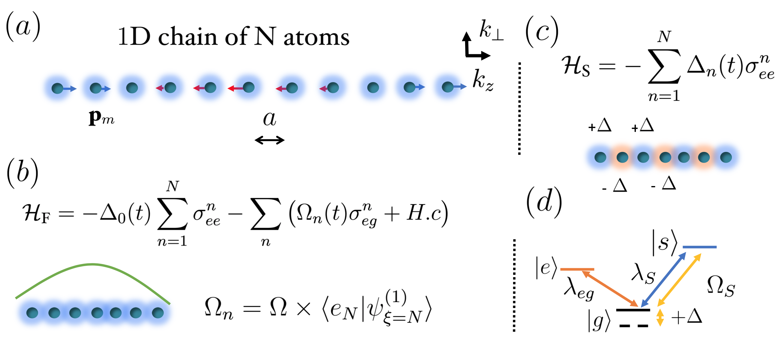
In this work, we explore a simple and robust physical system that could be built in a lab capable of absorbing, storing and emitting a photon with a temporal and spatial control. It consists in a linear chain of atoms with a total length larger than the wavelength to enable directivity and with a spacing smaller than half a wavelength to enhance interactions as represented in Fig. 1(a). It is composed of three-level atoms () located at positions . The frequency of the transition is given by and its polarization is considered linear and parallel to the chain. A second transition depicted in Fig. 1(d) exists between and with a transition frequency . The role of this transition is dual. First, it enables the optical trapping of the atoms with a nearest neighbor distance sufficiently small for subradiant modes to emerge. Second, it enables the realization of arbitrary detuning patterns [49] between the different atoms. It is a key point since the method we follow to manipulate collective states [45, 46] necessitate the realization of the so-called staggered pattern for which the local detuning of atom changes sign from site to site: . As a concrete example, we work with a conservative value of sufficiently small to create arbitrary PVD patterns and manipulate the subradiant modes that emerge in the atomic chain [46, 45]. This can be realized experimentally by loading an accordion lattice from an optical tweezer array [50].
III Theoretical model
We now introduce the model used to describe the light chain interaction. We use the Born and Markov approximation [51, 52] to integrate out the photonic degrees of freedom from the full atom-light system. This results in an interacting and open spin model, describing the dynamics of the atomic density matrix with the Master equation (M.E):
| (1) |
In this expression is the total Hamiltonian that includes : i) the effective Hamiltonian between the atoms from which collective subradiant and superradiant modes emerge, ii) the interacting Hamiltonian between the atoms and the excitation field and iii) the interacting Hamiltonian induced by a detuning pattern . Both the population recycling term and the effective Hamiltonian depend on the free space dyadic electromagnetic Green’s function , the vacuum permeability , the dipole of atom : , and with . We model the excitation of the atoms with an intense coherent pulse using: , with the detuning between the laser and atomic frequencies and the Rabi frequency of atom . We represent the application of the PVD using , with the local detuning of atom . When needed, we can turn off the excitation and/or the detuning pattern setting and/or to in Eq. (1).
III.1 Spectral properties of singly and doubly-excited states.
To simplify the analysis of Eq. (1), we sort the eigenstates of into different manifolds with a given number of excitations and use the superscript to label a given manifold. If for some specific reason, during the full dynamics, we truncate the Hilbert space to the populated manifolds only. Here, most of the results are presented with a numerical truncation of the Hilbert space to . This both reduces the computation time and simplifies the analysis to the first two manifolds that we briefly describe below.
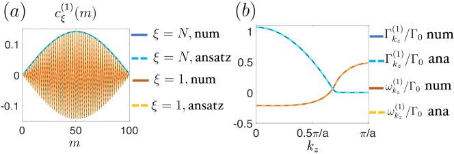
The diagonalization of in the first manifold results in eigenvectors such that where represents the shift in energy of with respect to and its decay rate. In order to differentiate easily the subradiant from the superradiant eigenmodes, we sort them from smallest to largest decay rate and label them with an integer denoted . For exemple, is the most subradiant mode of the chain while is the most superradiant. In Fig. 2(a), we plot the amplitude of on each atom for both the most superradiant () and subradiant singly-excited modes (). We see that the singly-excited eigenmodes of an ordered chain are spin waves, well represented by the ansatz: [26, 53]. Qualitatively, the most subradiant mode corresponds to a phase difference between nearest neighbors whereas the superradiant mode corresponds to a uniform phase across the chain. In Fig. 2(b), we compute the decay rate and the frequency shift of each eigenmode and plot them as a function of . We observe strong variations of the collective properties as a function of , in perfect agreement with the analytical expressions given in appendix A. In particular, Fig. 2(b) clarifies the physics of super and subradiance: spin waves with a wave vector along the chain larger than cannot couple to electromagnetic waves in vacuum and are strongly subradiant. On the opposite, superradiant modes are associated with small values of [54, 55, 56].
We now turn to the excited manifolds and consider states with two excitations. Due to the atomic nonlinearity, highly excited states are in general entangled, and very different from singly-excited ones [57, 58, 59, 60, 61, 62]. Yet, in the specific case of a D ordered atomic chain composed of atoms, the doubly-excited states can be built as an antisymmetric product of singly-excited spin waves [53, 56]. More precisely, we represent each doubly-excited state using the fermionic ansatz [53]: . In this expression, we used to label this state and note that it is identical to the state labeled with up to a minus sign. The consequence of the fermionic ansatz is that each doubly-excited state behaves like a doubly-excited spin wave, whose collective properties are well approximated by the sum of its single photon components: and . Let us conclude this section highlighting that the entanglement contained in the atomic degrees of freedom of a highly-excited state is an interesting resource whose extraction remains elusive for now [63, 59, 64, 65, 60, 66, 67]. A protocol, that permits the transfer of this entanglement to the emitted photons at a given time, and in a given direction would be key for quantum technologies.
IV Description of the protocol
We detail below the different steps of the protocol.
IV.1 Exciting the most superradiant mode.
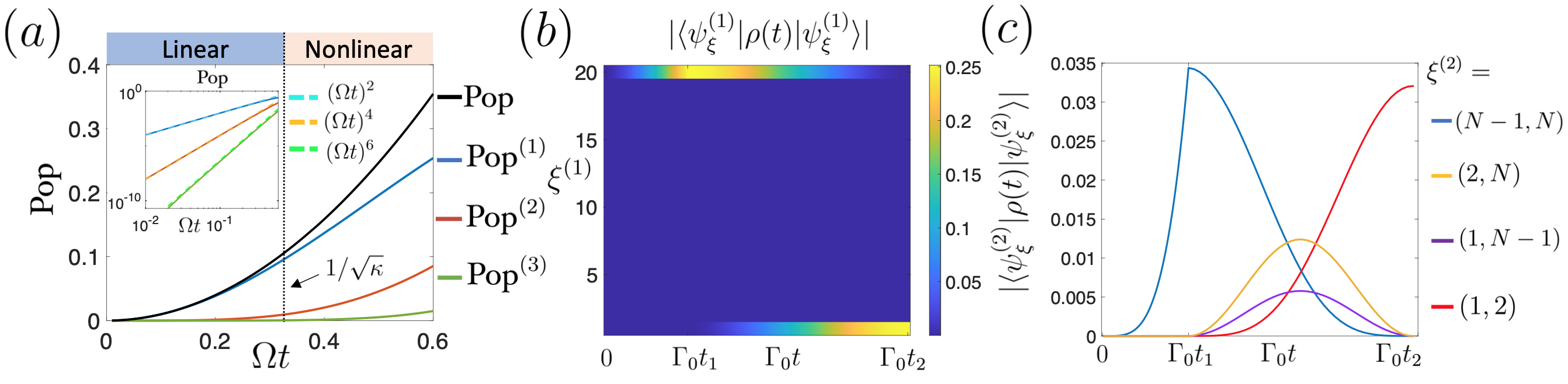
We start by illuminating transversally the atomic system from the far field with a strong () and monochromatic laser field resonant with the most superradiant singly-excited eigenmode: . The spatial profile of the incident field: is adjusted to couple preferentially the ground state to . This can be realized experimentally with state of the art SLM technologies. In Fig. 3(a) we study the populations in the first three manifolds when evolved with for . We see in the insert that the population with excitations denoted varies like . As a consequence, the single photon population dominates when . This is the so-called linear regime studied in [46, 45] that neglects the inherent nonlinearity of atoms. In this work, we illuminate the system for longer times and reach a regime where both and contribute to the dynamics (while keeping for the sake of computation time). In this nonlinear regime, our protocol benefits both from the increase of the total population in the chain, and from the possibility to harness the entanglement of doubly-excited states. Moreover, the wavefront shaping of the incident beam proposed in this work simplifies the dynamics lowering the number of populated eigenmodes. Indeed, we plot in Fig. 3(b) the projection of the density matrix onto each singly-excited eigenmode and observe that is fully carried by the superradiant state during the illumination: . In the second manifold, we observed numerically that the fermionic combination of the two most superradiant states largely dominates and contributes to of (see appendix C for an analytical justification).
IV.2 Transfer to the most subradiant modes.
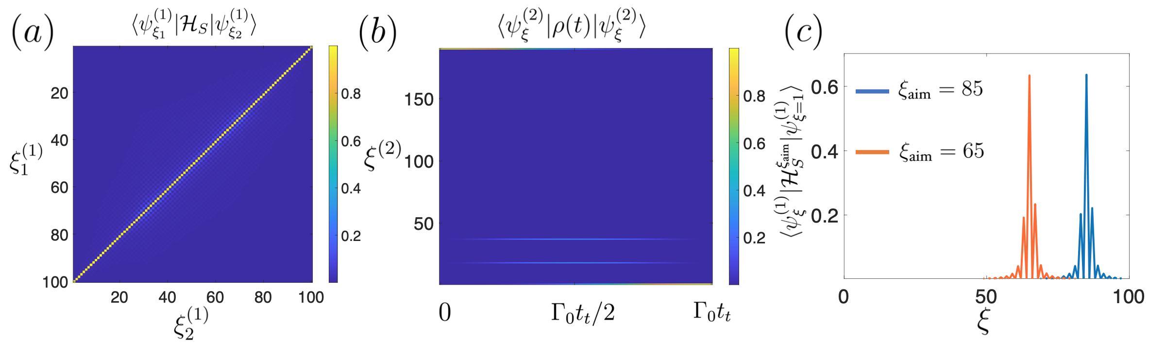
After an illumination time , we stop the driving field and turn on the PVD: . Since the eigenmodes of are different from the eigenmodes of the total hamilatonian , the application of the PVD induces a transfer of population between the different . In the specific case of the staggered pattern: , the matrix representation of in the singly-excited state basis of is perfectly anti-diagonal [see Fig. 7(a)]. This means that the application of this PVD induces a one-to-one coupling between and [46]. More precisely, in the reduced basis built with the coupling matrix writes:
| (2) |
In Fig. 3(b), we plot the projection of the density matrix onto each singly-excited eigenmode as a function of time during the first two steps of the protocol. At the beginning of the transfer (), is carried by . From to , we apply and observe a perfect transfer of the population to the most subradiant eigenmode . In the limit of a strong detuning: we can show that this transfer can be realized in a time small enough to neglect radiative loss.
Let us now push the analysis of the transfer to the two-photon population in the nonlinear regime. In this case, the coupling matrix in the complete doubly-excited state basis is harder to interpret visually. However, for a given initial state labeled with , the evolution happens in a space of dimension 4 expressed in terms of the labels for simplicity: . In this reduced basis, the transfer matrix has the form:
| (3) |
Since of the doubly-excited population is contained into the most superradiant doubly-excited state at the beginning of the transfer, we can restrict the discussion to the evolution of this specific eigenmode. The application of the staggered pattern first couples equally the most superradiant doubly-excited state to and . We note that these states are built with the anti-symmetric product of one super and one subradiant singly-excited eigenstates and could be used for the heralded creation of subradiant states. Those states are in turn coupled to which is the most subradiant doubly-excited state. In order to illustrate this discussion, we plot in Fig. 3(c) the projection of the density matrix onto those four doubly-excited states. Note that there is a factor of two between the projection of the density matrix onto a doubly-excited state and the atomic population that it induces as we deal with doubly-excited states. At the beginning of the transfer, we see in Fig. 3(c) that the projection of the density matrix is maximal onto the most superradiant doubly-excited state . It is then efficiently transferred to in the exact same time than derived for singly-excited states.
The application of the staggered pattern thus permits the coherent manipulation of doubly-excited states by switching their singly-excited components from superradiant to subradiant forms and vice-versa. We believe that the same phenomenon happens for larger excitation number () as soon as the generalization of the fermionic ansatz is valid. This work thus enlarges the coherent control of collective states using the staggerred pattern [46, 45] to higher manifolds.
IV.3 Storage.
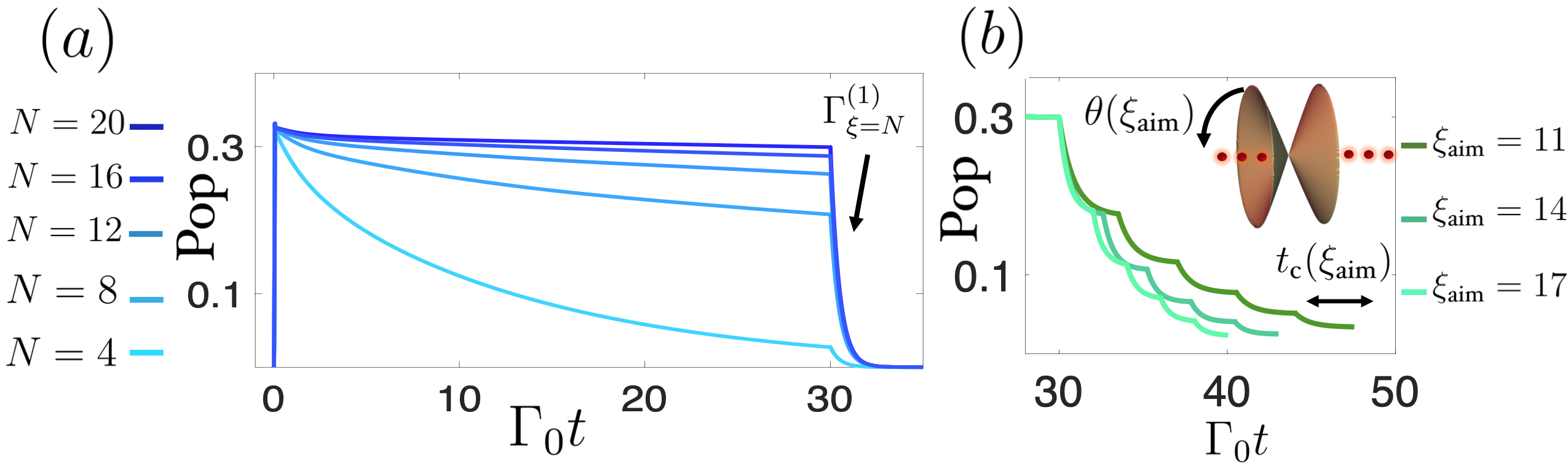
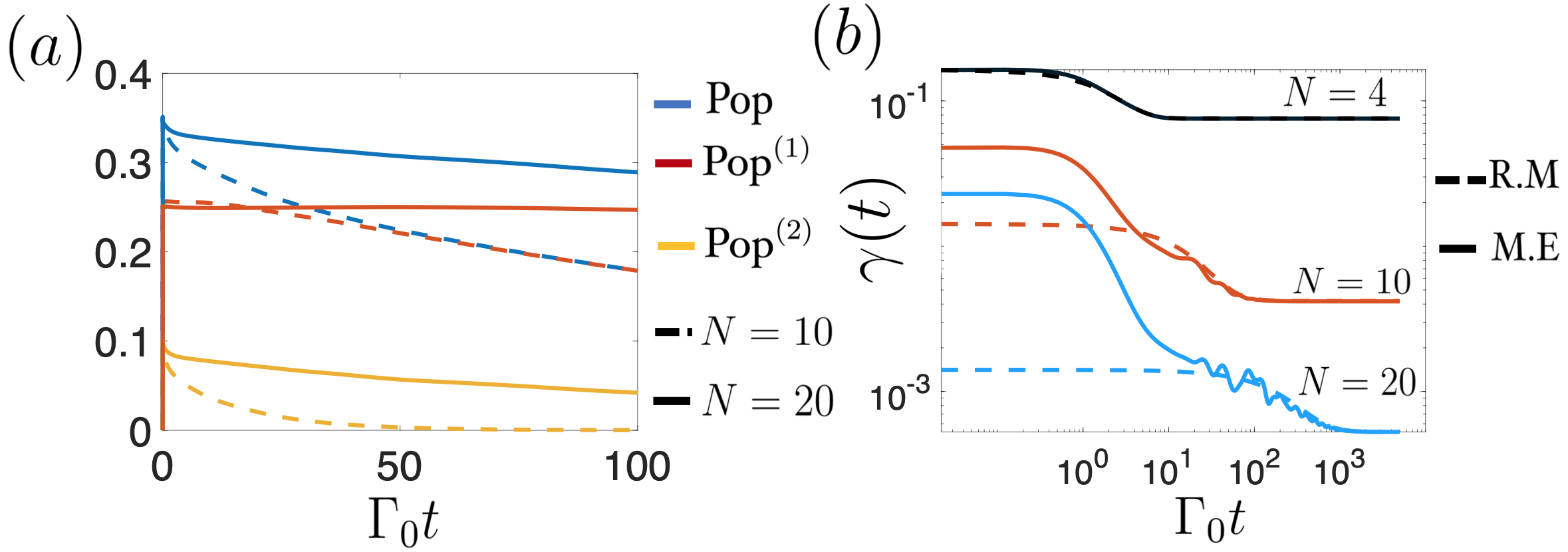
After a transfer time , we turn off and let the system evolve freely for sufficiently long times such that the loss term in Eq. (1) plays a role in the dynamics. In Fig. 4(a), we plot the total population in the chain during the complete protocol for various indicated by different colors. Due to the open character of the system, we observe a decrease of the atomic population during the storage (), which reveals that photons are emitted by the atomic chain. Importantly, we observe that the storage of the atomic population increases with the system size .
To discuss this first observation, we simplify the problem neglecting the of not contained into and approximate the state of the system at the end of the transfer by the pure state . Then, we follow [68] and use a rate model (R.M) described in appendices B and D that simplifies the analysis. Doing so, we restrict the the dynamics under free evolution in the presence of loss to a subspace built by the last two survivors and . This simplification leads to the following expression for the total atomic population:
| (4) |
where the first term of the right hand side represents and the second term . Since and are subradiant, both and decrease as . Injecting those scalings into Eq. (4) directly permits to recover the improvement of the storage of the total population when the system size increases observed numerically in Fig. 4(a).
Next, we push the analysis further comparing the rate of emission of photons coming from singly and doubly-excited states. To do so we study the instantaneous decay rate [69]:
| (5) |
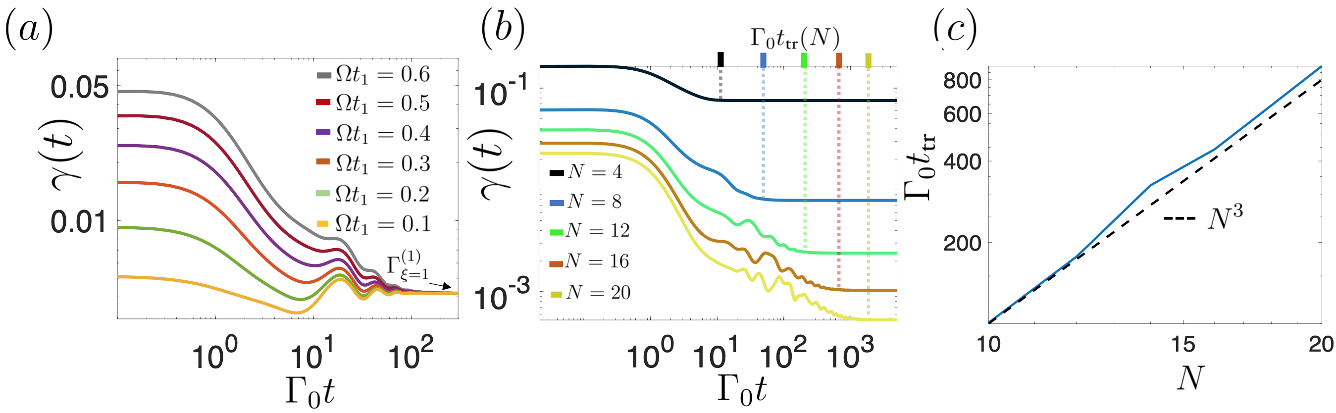
during the storage, for various and different values of . In Fig. 5(a) we plot the numerical value of for and varying from to . We see that whatever the value of , converges at ”long” times towards a plateau whose value is given by . This means that the emission of photons at ”long” times is dominated by single photons radiated by the most subradiant singly-excited state.
Next we turn to the study of the ”short” time regime of observed in Fig. 5(a) where varies with . To understand this point, we inject Eq. 4 into Eq. 5 and obtain a simplified expression of predicted by the R.M. It writes:
| (6) |
with the proportionality factor between and which comes from the fermionic ansatz [53]. In Fig. 8(b), we compare Eq. (6) with the exact calculation of using the M.E and observe that Eq. (6) slightly underestimates the instantaneous decay at short times. This comes from the neglect of the of not contained into . Nonetheless the R.M still captures the increase of when increases, and shows that this effect comes from the competition between the singly and doubly-excited decay. More importantly, we observe in Fig. 8(b) that Eq. (6) properly captures the dynamical transition between the short and long time regimes of . Hence the R.M permits to set the boundary between a short time regime where the emission is dominated by and a long time regime where it is dominated by . To do so, we introduce the transition time such as the time needed for to converge towards . We obtain its analytical expression using Eq. 6 using the condition that the weight of the single and two-photon decay should be equal at this specific time. We obtain:
| (7) |
with the ratio between the two decay rates almost constant to a value around for large systems (see Appendix D).
In Fig. 5(b), we fix , vary from to and extract the numerical value of that we project on top of the figure for the sake of clarity. In Fig. 5(c), we plot the extracted value of as a function of the system size and confirm numerically the variation of predicted by Eq. 7. This scaling shows that doubly-excited states dominate the emission for a time that strongly increases with the system size. Besides, Eq. 7 tells us that only exists if (due to the log). The condition depicted in Fig. 3(a) thus sets the boundary between the linear and the nonlinear regime (in terms of illumination strength) to . This order of magnitude is confirmed numerically in Fig. 5(a) in which we can estimate the minimum value of such that dominates the decay at short times to .
To conclude this section, we proposed a simplified model of the dynamics during the storage in order to compute the minimal value of the illumination strength needed to access the onset of the non-linear regime. In this regime, we showed that the two-photon population dominates the emission of photons for a duration that strongly increases with the system size.
IV.4 Emission.
After a sufficiently long storage time such that the two-photon population is completely negligible, the remaining population is fully carried by the most subradiant singly-excited state . On demand, one can turn on the PVD, transfer back the population to the most superradiant singly-excited mode in a time , and then let evolve the state with . Doing so, the atomic population decays at a rate , as observed in Fig. 4(a). In order to control the emission rate: , the frequency and the radiation pattern of the emitted single-photon, we introduce a new sinusoidal PVD:
| (8) |
that couples the most subradiant eigenmode to . As observed in Fig. 7(c) this coupling is not perfectly one-to-one, and rather looks like a sinc function. In order to avoid second order coupling to subradiant states which would prevent the efficient emission of the photon, we split the emission procedure in cycles. Each cycle contains one transfer step using the sinusoidal PVD of duration short enough for enabling first order coupling only, and one free evolution step of duration . This method enables the efficient emission of the photon mostly through the mode indexed as shown in Fig. 4(b). We compute the radiation pattern of the atomic ensemble using: with obtained from the resolution of eq. (1). The radiation pattern of one typical superradiant mode indexed with is given the inset of Fig. 4(b). For atoms linearly polarized along the chain, we see that the mode with label emits in a cone of angle that directly depends on : , with and . Perfect retrieval of the emitted single-photon can thus be realized with two lenses of proper NA.
V Conclusion
In summary, we studied theoretically a protocol that enables on-demand absorption, storage, and re-emission of an incident field using subradiant and superradiant states of an atomic chain. The three-level nature of the atoms allows both their trapping and manipulation using light shifts with a resolution smaller than . This permits the determistic coupling to subradiant states, which are important resources for metrology [70, 71] or quantum computing [72, 73]. Valid beyond the linear regime, our theoretical analysis provides an intuitive picture of the dynamics in terms of singly and doubly-excited states. For the first time to our knowledge, we discuss the manipulation of multiply excited states using tailored PVDs combined with shaped incident fields. We envision in the future to study the efficient excitation of highly excited states in order to control the quantum correlations of light emitted by the array [63, 67]. Quantum metamaterials [74, 75], such as D arrays have already been shown to act as a subradiant mirrors [24, 27, 44] or proposed to construct lossless D atomic waveguides [53, 76]. Adjusting their many-body functionalities on demand, in a time shorter than the emission time is a largely unexplored avenue that would enlarge their potential as versatile light-matter interfaces.
Acknowledgements
We acknowledge Ilan Shlesinger and Jean-Paul Hugonin for important discussions. A.B. and I.F-B acknowledge funding from the European Research Council (Grants. No. 101018511, ATARAXIA, 101039361, CORSAIR) and by the Agence National de la Recherche (ANR, project DEAR).
Appendix A
Collective properties of singly-excited states
In this appendix, we remind the analytical expressions of and derived in the literature [53, 26] in order to understand the collective properties of the eigenmodes of the effective Hamiltonian. can be expressed in terms of the reciprocal lattice vectors , and writes (for a linear atomic polarization along the chain):
| (9) |
The analytical expression of can be obtained using the mathematical function , and . It writes:
| (10) |
We stress here that those quantities depends on the atomic polarization. The numerical results presented in this work have been derived for a linear polarization along the chain. However, they can be easily extended to the same system with circular atomic polarization simply by adapting the exact value of the decay rates and the frequency shifts [53, 26]. For an atomic polarization linear and orthogonal to the chain (along for instance), the link between and is more involved, but the physics of super and subradiance remains the same. Namely, spin waves with a wave vector along the chain larger than cannot couple to electromagnetic waves in vacuum and are strongly subradiant. On the opposite, superradiant modes are associated with small values of .
Appendix B Decay of the doubly-excited eigenmodes
In this appendix, we remind some properties of the most super and subradiant doubly-excited states useful to understand the population dynamics during the protocol in the nonlinear regime. The most subradiant (respectively superradiant) doubly-excited eigenmode is built as a fermionic product of singly-excited states with indexes [respectively ]. As a direct consequence, the most superradiant doubly-excited eigenmode mostly decays into the singly-excited states of indexes and while the most subradiant decays into and [68]. The reduction of the number of states involved in the decay process enables the use of a simplified rate model involving only 3 different states: :
| (11) |
with the population of the doubly-excited mode, and the population of the singly-excited modes into which it decays. The decay rate from state to state can be computed using , with the recycling operator of the M.E given in Eq. (1) of the main text.
Appendix C Details of the steps of the protocol
C.1 Coupling with the field
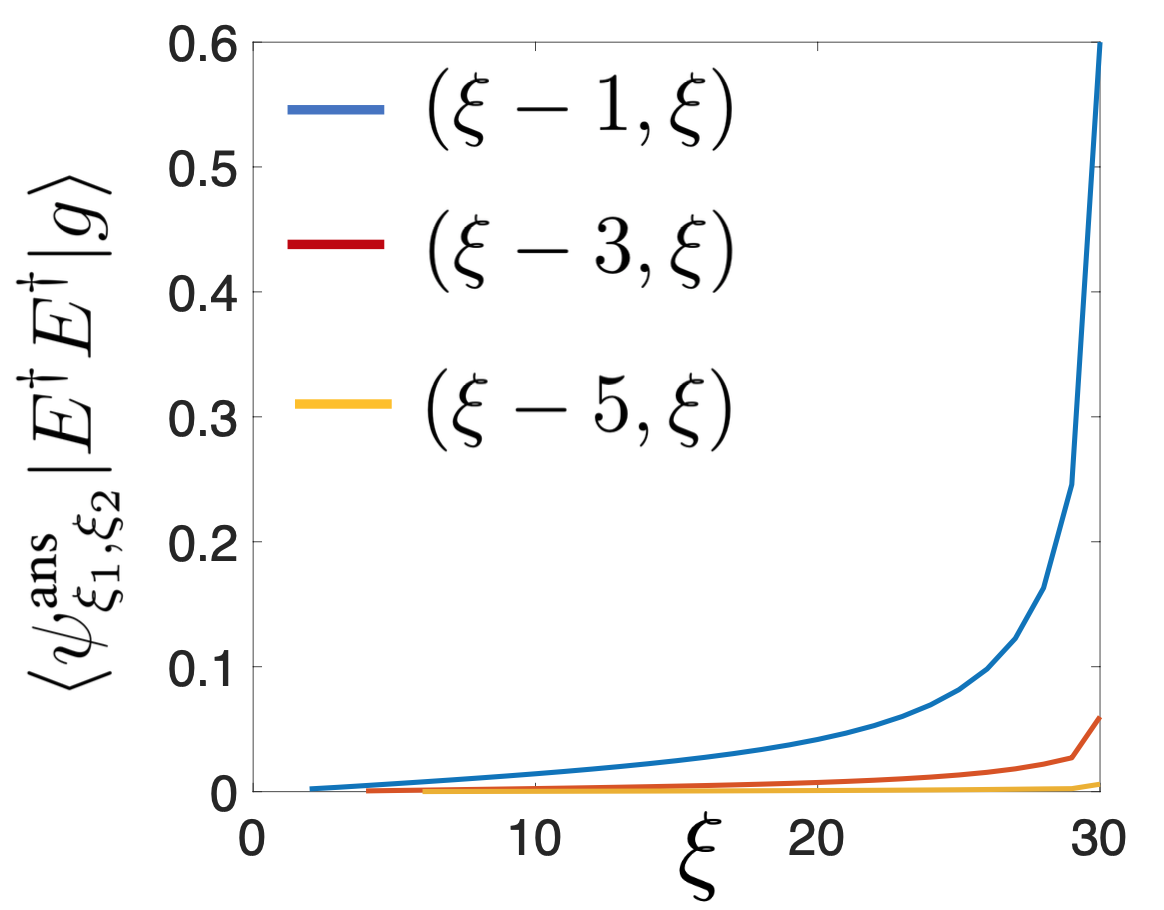
We chose the field operator in order to couple the ground state to efficiently. Indeed, one can check numerically or analytically that . However we do not know a priori which doubly-excited eigenstates are populated when the field operator is applied twice to the ground state and creates . To identify this state, we take its dot product with every two-photon ansatz states: using:
| (12) |
with a normalization factor and the singly-excited eigenmode ansatz. This leads to a rather long expression:
| (13) |
that we evaluate numerically in Fig. 6. We show that, when applied two times on the ground state, the field preferentially couples to : the most superradiant doubly-excited state. One should note that a part of the two-photon population is carried by other modes ( of the two-photon population observed numerically). This of is responsible for the discrepancy observed at short times in the evaluation of using the R.M and the M.E observed in Fig. 8(b).
C.2 Modes transfer using PVD
In this subsection, we provide additional details about mode transfer using PVD. In Fig. 7(a) we represent and observe an almost perfect anti-diagonal matrix. This means that, the evolution of an eigenmode with label of under the application of the staggered pattern happens in a space of dimension : .
In the second manifold, we choose not to represent the matrix elements as they are difficult to interpret visually. Instead, we plot in Fig. 7(b) the projection of the density matrix onto each doubly-excited eigenmode during the transfer. In this plot, is not a 2D vector but a number that sorts the doubly-excited eigenmodes with respect to their decay rate. The initial state is the most superradiant doubly-excited state associated with (for atoms). It is then equally transferred to the doubly-excited state of index (built with the product of and ) and the doubly-excited state of index (built with the product of and ). Eventually, those two modes are coupled to the most subradiant doubly-excited state associated with (built with the product of and ).
At the end of the storage, we want to transfer back the singly-excited subradiant state into the superradiant mode of our choice. Thus, we use the following sinusoidal PVD: with . This detuning pattern mostly couples the most subradiant mode () to the eigenstate with label as observed in Fig. 7(c). However, since the coupling is not one to one (it rather looks like a sinc function), the emission protocol should be split into cycles. Each cycle contains one transfer step using the sinusoidal PVD of duration and one free evolution step of duration . With this method, we can funnel most of the emission through the singly-excited eigenmode with label and avoid residual coupling to subradiant eigenmodes.
Appendix D Last two survivors approximation
In this section, we provide additional details about the analysis of the role of the two-photon population during the storage. As a first observation, we plot in Fig. 8(a) the total population (blue), the population of the single photon components (red) and two-photons components (yellow) for two different system sizes ( in dashed and in solid lines) for . We observe that both the single and the two-photon components are better stored as increases and clearly observe that the two-photon population can not be neglected for ”short” times.
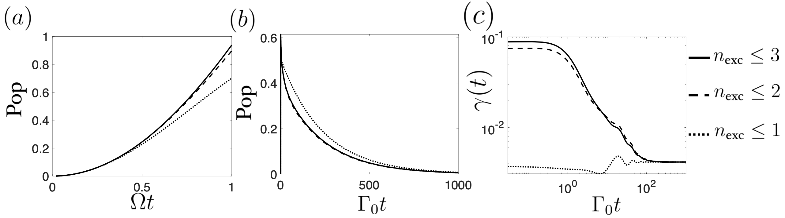
In Fig. 8(b) we compare the value of given by the R.M and by the M.E. We observe a good agreement for both the long time value of and as discussed in the main text. This shows that we can use the reduced set of states of the R.M: to compute the dynamics for . To do so, we express the total population during the storage in the reduced basis:
| (14) |
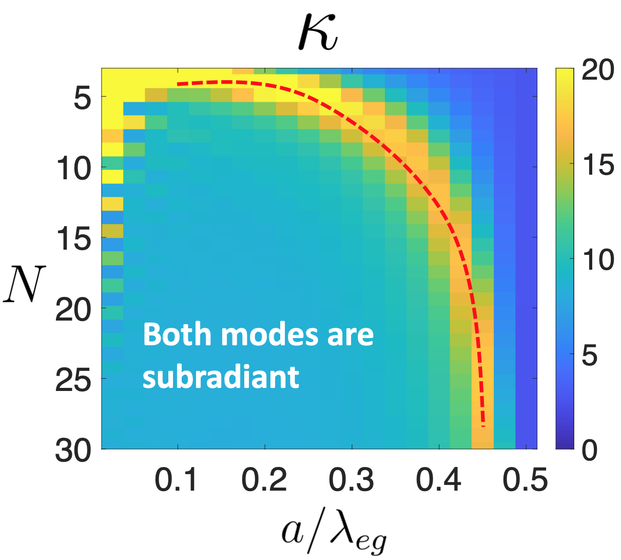
with , and the population of the three modes involved. Their initial values at (beginning of the storage) depend on : , and and their dynamics can be solved numerically using eq. 11. In this specific study of the transition time , plays a negligible role as both its population and decay rate are low. We thus reduce the analytical analysis to the last two survivors and , neglect the filling of due to the decay of in order to obtain the simplified expression of the total population provided in Eq. 4. Equation 4 is written in terms of and , which are the decay rates of the most subradiant singly and doubly-excited states. represents the ratio between the two decay rates: . In Fig. 9, we plot its numerical value as a function of and . In the regime where both modes are subradiant, is found to be almost constant to a value around .
Appendix E Justification of the truncation of the Hilbert space to in the nonlinear regime
In this appendix we justify the validity of the numerical truncation of the Hilbert space up to for the study of the total population and the instantaneous decay rate. In Fig. 10(a,b) we plot the total population in the chain computed with a numerical truncation of the Hilbert space going from to (in black solid, dashed and pointed lines). Let us denote the total population computed with a numerical truncation up to . We observe that and are very similar during the illumination (a) and the storage (b) steps of the protocol. This demonstrates that the numerical truncation to is enough to properly represent the total population in the system during the different steps of our protocol in the limit of low three-photon population defined as .
Let us now justify the validity of the numerical truncation to in the analysis of . To do so we plot in Fig. 10(c) the numerical value of during the storage computed with a numerical truncation of the Hilbert space from to . We see that all curves have the same long time limit (given by the decay rate of the most subradiant singly-excited state). However, it appears that the reduction of the analysis to creates a strong error in the short time behavior of the instantaneous decay rate. By contrast, comparing for and , we see that the presence of a three-photon population only slightly modifies the instantaneous decay rate for times shorter than . From this analysis, we conclude that we can neglect the tiny three-photon population (and higher manifolds), in the analysis of the made in the nonlinear regime.
References
- Hammerer et al. [2010] K. Hammerer, A. S. Sørensen, and E. S. Polzik, Quantum interface between light and atomic ensembles, Reviews of Modern Physics 82, 1041 (2010).
- Raimond et al. [2001] J.-M. Raimond, M. Brune, and S. Haroche, Manipulating quantum entanglement with atoms and photons in a cavity, Reviews of Modern Physics 73, 565 (2001).
- Saffman et al. [2010] M. Saffman, T. G. Walker, and K. Mølmer, Quantum information with rydberg atoms, Reviews of Modern Physics 82, 2313 (2010).
- Kimble [2008] H. J. Kimble, The quantum internet, Nature 453, 1023 (2008).
- Thompson et al. [2013] J. D. Thompson, T. Tiecke, N. P. de Leon, J. Feist, A. Akimov, M. Gullans, A. S. Zibrov, V. Vuletić, and M. D. Lukin, Coupling a single trapped atom to a nanoscale optical cavity, Science 340, 1202 (2013).
- Reiserer and Rempe [2015] A. Reiserer and G. Rempe, Cavity-based quantum networks with single atoms and optical photons, Reviews of Modern Physics 87, 1379 (2015).
- Plankensteiner et al. [2017] D. Plankensteiner, C. Sommer, H. Ritsch, and C. Genes, Cavity antiresonance spectroscopy of dipole coupled subradiant arrays, Physical Review Letters 119, 093601 (2017).
- Shlesinger et al. [2021] I. Shlesinger, P. Senellart, L. Lanco, and J.-J. Greffet, Time-frequency encoded single-photon generation and broadband single-photon storage with a tunable subradiant state, Optica 8, 95 (2021).
- Lei et al. [2023] M. Lei, R. Fukumori, J. Rochman, B. Zhu, M. Endres, J. Choi, and A. Faraon, Many-body cavity quantum electrodynamics with driven inhomogeneous emitters, Nature , 1 (2023).
- Nayak et al. [2007] K. Nayak, P. Melentiev, M. Morinaga, F. Le Kien, V. Balykin, and K. Hakuta, Optical nanofiber as an efficient tool for manipulating and probing atomic fluorescence, Optics Express 15, 5431 (2007).
- Solano et al. [2017] P. Solano, P. Barberis-Blostein, F. K. Fatemi, L. A. Orozco, and S. L. Rolston, Super-radiance reveals infinite-range dipole interactions through a nanofiber, Nature communications 8, 1 (2017).
- Corzo et al. [2019] N. V. Corzo, J. Raskop, A. Chandra, A. S. Sheremet, B. Gouraud, and J. Laurat, Waveguide-coupled single collective excitation of atomic arrays, Nature 566, 359 (2019).
- Pennetta et al. [2022] R. Pennetta, M. Blaha, A. Johnson, D. Lechner, P. Schneeweiss, J. Volz, and A. Rauschenbeutel, Collective radiative dynamics of an ensemble of cold atoms coupled to an optical waveguide, Physical Review Letters 128, 073601 (2022).
- Goban et al. [2014] A. Goban, C.-L. Hung, S.-P. Yu, J. Hood, J. Muniz, J. Lee, M. Martin, A. McClung, K. Choi, D. E. Chang, et al., Atom–light interactions in photonic crystals, Nature communications 5, 1 (2014).
- Goban et al. [2015] A. Goban, C.-L. Hung, J. Hood, S.-P. Yu, J. Muniz, O. Painter, and H. Kimble, Superradiance for atoms trapped along a photonic crystal waveguide, Physical Review Letters 115, 063601 (2015).
- Lodahl et al. [2015] P. Lodahl, S. Mahmoodian, and S. Stobbe, Interfacing single photons and single quantum dots with photonic nanostructures, Reviews of Modern Physics 87, 347 (2015).
- Yu et al. [2014] S.-P. Yu, J. Hood, J. Muniz, M. Martin, R. Norte, C.-L. Hung, S. M. Meenehan, J. D. Cohen, O. Painter, and H. Kimble, Nanowire photonic crystal waveguides for single-atom trapping and strong light-matter interactions, Applied Physics Letters 104, 111103 (2014).
- Fayard et al. [2022] N. Fayard, A. Bouscal, J. Berroir, A. Urvoy, T. Ray, S. Mahapatra, M. Kemiche, J. A. Levenson, J.-J. Greffet, K. Bencheikh, J. Laurat, and C. Sauvan, Asymmetric comb waveguide for strong interactions between atoms and light, Opt. Express 30, 45093 (2022).
- Bouscal et al. [2023] A. Bouscal, M. Kemiche, S. Mahapatra, N. Fayard, J. Berroir, T. Ray, J.-J. Greffet, F. Raineri, A. Levenson, K. Bencheikh, et al., Systematic design of a robust half-w1 photonic crystal waveguide for interfacing slow light and trapped cold atoms, arXiv preprint arXiv:2301.04675 (2023).
- Turchette et al. [1995] Q. A. Turchette, C. J. Hood, W. Lange, H. Mabuchi, and H. J. Kimble, Measurement of conditional phase shifts for quantum logic, Physical Review Letters 75, 4710 (1995).
- Chang et al. [2014] D. E. Chang, V. Vuletić, and M. D. Lukin, Quantum nonlinear optics—photon by photon, Nature Photonics 8, 685 (2014).
- Roy et al. [2017] D. Roy, C. M. Wilson, and O. Firstenberg, Colloquium: Strongly interacting photons in one-dimensional continuum, Reviews of Modern Physics 89, 021001 (2017).
- Sheremet et al. [2023] A. S. Sheremet, M. I. Petrov, I. V. Iorsh, A. V. Poshakinskiy, and A. N. Poddubny, Waveguide quantum electrodynamics: collective radiance and photon-photon correlations, Reviews of Modern Physics 95, 015002 (2023).
- Bettles et al. [2016] R. J. Bettles, S. A. Gardiner, and C. S. Adams, Enhanced optical cross section via collective coupling of atomic dipoles in a 2d array, Physical Review Letters 116, 103602 (2016).
- Facchinetti et al. [2016] G. Facchinetti, S. D. Jenkins, and J. Ruostekoski, Storing light with subradiant correlations in arrays of atoms, Physical Review Letters 117, 243601 (2016).
- Shahmoon et al. [2017] E. Shahmoon, D. S. Wild, M. D. Lukin, and S. F. Yelin, Cooperative resonances in light scattering from two-dimensional atomic arrays, Physical Review Letters 118, 113601 (2017).
- Rui et al. [2020] J. Rui, D. Wei, A. Rubio-Abadal, S. Hollerith, J. Zeiher, D. M. Stamper-Kurn, C. Gross, and I. Bloch, A subradiant optical mirror formed by a single structured atomic layer, Nature 583, 369 (2020).
- Dicke [1954] R. H. Dicke, Coherence in spontaneous radiation processes, Physical review 93, 99 (1954).
- Gross and Haroche [1982] M. Gross and S. Haroche, Superradiance: An essay on the theory of collective spontaneous emission, Physics reports 93, 301 (1982).
- Scully et al. [2006] M. O. Scully, E. S. Fry, C. R. Ooi, and K. Wódkiewicz, Directed spontaneous emission from an extended ensemble of n atoms: Timing is everything, Physical Review Letters 96, 010501 (2006).
- Araújo et al. [2016] M. O. Araújo, I. Krešić, R. Kaiser, and W. Guerin, Superradiance in a large and dilute cloud of cold atoms in the linear-optics regime, Physical Review Letters 117, 073002 (2016).
- He et al. [2020a] Y. He, L. Ji, Y. Wang, L. Qiu, J. Zhao, Y. Ma, X. Huang, S. Wu, and D. E. Chang, Atomic spin-wave control and spin-dependent kicks with shaped subnanosecond pulses, Physical Review Research 2, 043418 (2020a).
- He et al. [2020b] Y. He, L. Ji, Y. Wang, L. Qiu, J. Zhao, Y. Ma, X. Huang, S. Wu, and D. E. Chang, Geometric control of collective spontaneous emission, Physical Review Letters 125, 213602 (2020b).
- Rastogi et al. [2022] A. Rastogi, E. Saglamyurek, T. Hrushevskyi, and L. J. LeBlanc, Superradiance-mediated photon storage for broadband quantum memory, Physical Review Letters 129, 120502 (2022).
- Scully [2015] M. O. Scully, Single photon subradiance: quantum control of spontaneous emission and ultrafast readout, Physical Review Letters 115, 243602 (2015).
- Plankensteiner et al. [2015] D. Plankensteiner, L. Ostermann, H. Ritsch, and C. Genes, Selective protected state preparation of coupled dissipative quantum emitters, Scientific reports 5, 1 (2015).
- Guerin et al. [2016] W. Guerin, M. O. Araújo, and R. Kaiser, Subradiance in a large cloud of cold atoms, Physical Review Letters 116, 083601 (2016).
- Cipris et al. [2021] A. Cipris, N. A. Moreira, T. do Espirito Santo, P. Weiss, C. Villas-Boas, R. Kaiser, W. Guerin, and R. Bachelard, Subradiance with saturated atoms: population enhancement of the long-lived states, Physical Review Letters 126, 103604 (2021).
- Ferioli et al. [2021] G. Ferioli, A. Glicenstein, L. Henriet, I. Ferrier-Barbut, and A. Browaeys, Storage and release of subradiant excitations in a dense atomic cloud, Physical Review X 11, 021031 (2021).
- Bloch et al. [2012] I. Bloch, J. Dalibard, and S. Nascimbene, Quantum simulations with ultracold quantum gases, Nature Physics 8, 267 (2012).
- Nogrette et al. [2014] F. Nogrette, H. Labuhn, S. Ravets, D. Barredo, L. Béguin, A. Vernier, T. Lahaye, and A. Browaeys, Single-atom trapping in holographic 2d arrays of microtraps with arbitrary geometries, Physical Review X 4, 021034 (2014).
- Endres et al. [2016] M. Endres, H. Bernien, A. Keesling, H. Levine, E. R. Anschuetz, A. Krajenbrink, C. Senko, V. Vuletic, M. Greiner, and M. D. Lukin, Atom-by-atom assembly of defect-free one-dimensional cold atom arrays, Science 354, 1024 (2016).
- Barredo et al. [2016] D. Barredo, S. De Léséleuc, V. Lienhard, T. Lahaye, and A. Browaeys, An atom-by-atom assembler of defect-free arbitrary two-dimensional atomic arrays, Science 354, 1021 (2016).
- Srakaew et al. [2023] K. Srakaew, P. Weckesser, S. Hollerith, D. Wei, D. Adler, I. Bloch, and J. Zeiher, A subwavelength atomic array switched by a single rydberg atom, Nature Physics , 1 (2023).
- Ballantine and Ruostekoski [2021] K. Ballantine and J. Ruostekoski, Quantum single-photon control, storage, and entanglement generation with planar atomic arrays, PRX Quantum 2, 040362 (2021).
- Rubies-Bigorda et al. [2022] O. Rubies-Bigorda, V. Walther, T. L. Patti, and S. F. Yelin, Photon control and coherent interactions via lattice dark states in atomic arrays, Physical Review Research 4, 013110 (2022).
- Norcia et al. [2018] M. Norcia, A. Young, and A. Kaufman, Microscopic control and detection of ultracold strontium in optical-tweezer arrays, Physical Review X 8, 041054 (2018).
- Saskin et al. [2019] S. Saskin, J. Wilson, B. Grinkemeyer, and J. Thompson, Narrow-line cooling and imaging of ytterbium atoms in an optical tweezer array, Physical Review Letters 122, 143002 (2019).
- de Léséleuc et al. [2017] S. de Léséleuc, D. Barredo, V. Lienhard, A. Browaeys, and T. Lahaye, Optical control of the resonant dipole-dipole interaction between rydberg atoms, Physical Review Letters 119, 053202 (2017).
- Ville et al. [2017] J. Ville, T. Bienaimé, R. Saint-Jalm, L. Corman, M. Aidelsburger, L. Chomaz, K. Kleinlein, D. Perconte, S. Nascimbène, J. Dalibard, et al., Loading and compression of a single two-dimensional bose gas in an optical accordion, Physical Review A 95, 013632 (2017).
- Reitz et al. [2022] M. Reitz, C. Sommer, and C. Genes, Cooperative quantum phenomena in light-matter platforms, PRX Quantum 3, 010201 (2022).
- Agarwal [2012] G. S. Agarwal, Quantum optics (Cambridge University Press, 2012).
- Asenjo-Garcia et al. [2017] A. Asenjo-Garcia, M. Moreno-Cardoner, A. Albrecht, H. Kimble, and D. E. Chang, Exponential improvement in photon storage fidelities using subradiance and “selective radiance” in atomic arrays, Physical Review X 7, 031024 (2017).
- Manzoni et al. [2018] M. Manzoni, M. Moreno-Cardoner, A. Asenjo-Garcia, J. V. Porto, A. V. Gorshkov, and D. Chang, Optimization of photon storage fidelity in ordered atomic arrays, New journal of physics 20, 083048 (2018).
- Zhang and Mølmer [2019] Y.-X. Zhang and K. Mølmer, Theory of subradiant states of a one-dimensional two-level atom chain, Physical Review Letters 122, 203605 (2019).
- Zhang and Mølmer [2020] Y.-X. Zhang and K. Mølmer, Subradiant emission from regular atomic arrays: Universal scaling of decay rates from the generalized bloch theorem, Physical Review Letters 125, 253601 (2020).
- Chang et al. [2018] D. Chang, J. Douglas, A. González-Tudela, C.-L. Hung, and H. Kimble, Colloquium: Quantum matter built from nanoscopic lattices of atoms and photons, Reviews of Modern Physics 90, 031002 (2018).
- Zhang et al. [2020] Y.-X. Zhang, C. Yu, and K. Mølmer, Subradiant bound dimer excited states of emitter chains coupled to a one dimensional waveguide, Physical Review Research 2, 013173 (2020).
- Bettles et al. [2020] R. J. Bettles, M. D. Lee, S. A. Gardiner, and J. Ruostekoski, Quantum and nonlinear effects in light transmitted through planar atomic arrays, Communications Physics 3, 141 (2020).
- Moreno-Cardoner et al. [2021] M. Moreno-Cardoner, D. Goncalves, and D. E. Chang, Quantum nonlinear optics based on two-dimensional rydberg atom arrays, Physical Review Letters 127, 263602 (2021).
- Fayard et al. [2021] N. Fayard, L. Henriet, A. Asenjo-Garcia, and D. Chang, Many-body localization in waveguide quantum electrodynamics, Physical Review Research 3, 033233 (2021).
- Holzinger et al. [2022] R. Holzinger, R. Gutiérrez-Jáuregui, T. Hönigl-Decrinis, G. Kirchmair, A. Asenjo-Garcia, and H. Ritsch, Control of localized single-and many-body dark states in waveguide qed, Physical Review Letters 129, 253601 (2022).
- Masson et al. [2020] S. J. Masson, I. Ferrier-Barbut, L. A. Orozco, A. Browaeys, and A. Asenjo-Garcia, Many-body signatures of collective decay in atomic chains, Physical Review Letters 125, 263601 (2020).
- Cidrim et al. [2020] A. Cidrim, T. do Espirito Santo, J. Schachenmayer, R. Kaiser, and R. Bachelard, Photon blockade with ground-state neutral atoms, Physical Review Letters 125, 073601 (2020).
- Williamson et al. [2020] L. Williamson, M. O. Borgh, and J. Ruostekoski, Superatom picture of collective nonclassical light emission and dipole blockade in atom arrays, Physical review letters 125, 073602 (2020).
- Zhang et al. [2022] L. Zhang, V. Walther, K. Mølmer, and T. Pohl, Photon-photon interactions in rydberg-atom arrays, Quantum 6, 674 (2022).
- Richter et al. [2023] S. Richter, S. Wolf, J. von Zanthier, and F. Schmidt-Kaler, Collective photon emission of two correlated atoms in free space, Physical Review Research 5, 013163 (2023).
- Henriet et al. [2019] L. Henriet, J. S. Douglas, D. E. Chang, and A. Albrecht, Critical open-system dynamics in a one-dimensional optical-lattice clock, Physical Review A 99, 023802 (2019).
- Rubies-Bigorda et al. [2023] O. Rubies-Bigorda, S. Ostermann, and S. F. Yelin, Dynamic population of multiexcitation subradiant states in incoherently excited atomic arrays, Physical Review A 107, L051701 (2023).
- Ostermann et al. [2013] L. Ostermann, H. Ritsch, and C. Genes, Protected state enhanced quantum metrology with interacting two-level ensembles, Physical Review Letters 111, 123601 (2013).
- Facchinetti and Ruostekoski [2018] G. Facchinetti and J. Ruostekoski, Interaction of light with planar lattices of atoms: Reflection, transmission, and cooperative magnetometry, Physical Review A 97, 023833 (2018).
- Wild et al. [2018] D. S. Wild, E. Shahmoon, S. F. Yelin, and M. D. Lukin, Quantum nonlinear optics in atomically thin materials, Physical Review Letters 121, 123606 (2018).
- Guimond et al. [2019] P.-O. Guimond, A. Grankin, D. Vasilyev, B. Vermersch, and P. Zoller, Subradiant bell states in distant atomic arrays, Physical Review Letters 122, 093601 (2019).
- Bekenstein et al. [2020] R. Bekenstein, I. Pikovski, H. Pichler, E. Shahmoon, S. F. Yelin, and M. D. Lukin, Quantum metasurfaces with atom arrays, Nature Physics 16, 676 (2020).
- Solntsev et al. [2021] A. S. Solntsev, G. S. Agarwal, and Y. S. Kivshar, Metasurfaces for quantum photonics, Nature Photonics 15, 327 (2021).
- Masson and Asenjo-Garcia [2020] S. J. Masson and A. Asenjo-Garcia, Atomic-waveguide quantum electrodynamics, Physical Review Research 2, 043213 (2020).