RME-GAN: A Learning Framework for Radio Map Estimation based on Conditional Generative Adversarial Network

Abstract

Outdoor radio map estimation is an important tool for network planning and resource management in modern Internet of Things (IoT) and cellular systems. Radio map describes spatial signal strength distribution and provides network coverage information. A practical goal is to estimate fine-resolution radio maps from sparse radio strength measurements. However, non-uniformly positioned measurements and access obstacles can make it difficult for accurate radio map estimation (RME) and spectrum planning in many outdoor environments. In this work, we develop a two-phase learning framework for radio map estimation by integrating radio propagation model and designing a conditional generative adversarial network (cGAN). We first explore global information to extract the radio propagation patterns. We then focus on the local features to estimate the effect of shadowing on radio maps in order to train and optimize the cGAN. Our experimental results demonstrate the efficacy of the proposed framework for radio map estimation based on generative models from sparse observations in outdoor scenarios.

I Introduction

The rapid development of information technologies has spawned many novel concepts and applications, such as the Internet of Things (IoT), autonomous driving, and cellular networks. For these wireless services, efficient spectrum planning and network coverage analysis are critical to spectrum efficiency and user experience. Specifically, radio maps provide vital information on spatial distribution of radio frequency (RF) signal power, and facilitate resource allocation and network outage diagnosis [1]. In general, RF ‘radio map’ refers to a geographical signal power spectrum density (PSD), formed by cumulative received RF signal power, as a function of spatial locations and frequencies, and may also exhibit temporal variations [2]. Enriching useful information on propagation behavior and spectrum occupancy, radio map could provide more detailed information on PSD distribution [3] spatially, shown as Fig. 1(a). However, RF signal powers can only be sparsely measured in practice. Thus, a practical challenge is the estimation of fine-resolution radio map from spatially sparse signal power samples collected by sensors or user devices as shown in Fig. 1(b). Our goal here is to achieve more efficient and accurate estimation of radio maps from sparse observations.

(a) Radio Map over Different Locations

(b) Sparse Samples Collected by Sensors

Figure 1: Example of Radio Map: a) radio map generated from simulators with three transmitters; b) 1000 samples from the original radio map.

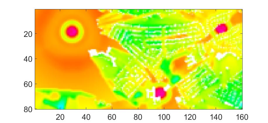
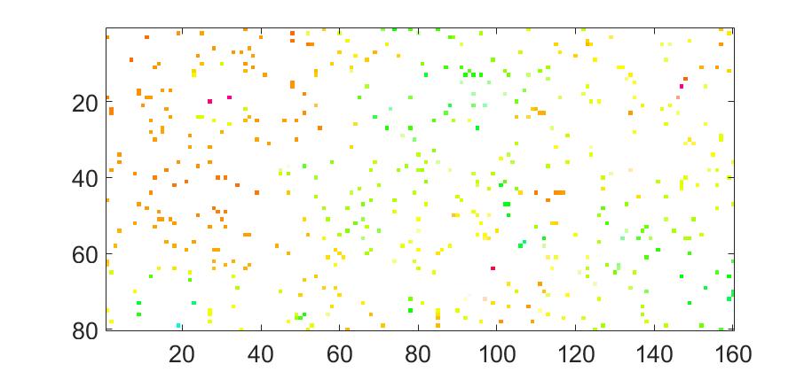
Most current approaches to radiomap estimation (reconstruction) can be categorized into either model-based or model-free. Model-based methods usually assume certain signal propagation models and express the received signal PSD as a combination from active transmitters [2]. For example, the authors of [4] introduced log-distance path loss model (LDPL) for Wi-Fi radio map reconstruction. In [5], another model-based method proposed interpolation based on thin-plate splines kernels. On the other hand, model-free methods do not assume a specific model but explore more neighborhood information. Typical examples include Radial Basis Function (RBF) [6] interpolation and inverse distance weighted (IDW) interpolation [7]. In addition to interpolation methods, there have also been a number of works that apply machine learning for radio map reconstruction. The authors of [8] presented a fast radio map estimation based on Unet [9]. Another team [10] proposed deep auto-encoders for estimating geographical PSD distribution. We will provide a more complete literature review later in Section II.

Despite many successes, existing solutions still exhibit certain limitations. First, unlike the problem of astronomical image analysis [11] and 3D city map reconstruction [12], ground truth radio map is more sensitive to the complex environment beyond mere radio propagation models. Failure to capture effects from shadowing or obstacles limits the efficacy of model-based approaches. On the other hand, the performance of model-free methods relies on the quality of observed samples. Generally, they assume a uniform distribution of measurements over the geometric space. However, in practical applications such as minimization of drive test (MDT) [13], measurements are collected from user devices, which are typically non-uniformly distributed within cell coverage. It is a challenge to process unevenly distributed observations efficiently. Moreover, samples in different training sets do not necessarily have the same radio propagation models and parameters. In view of their respective strengths and shortcomings, we should consider effective integration of model-based and model-free methods.

To address the aforementioned problems, we investigate radio propagation in the outdoor scenario, and propose a two-phase learning framework (RME-GAN) for radio map estimation based on conditional generative adversarial networks (cGAN) [14]. Since a radio map can be dynamically constructed from real-time measures and continuously updated [2], we mainly focus on the step of radio map estimation from sparse observations over geographical locations. In phase 1, we integrate learning-based and model-based principles to extract global information while leveraging radio propagation model. In phase 2, we utilize different sampling strategies to capture local radiomap features and to explore the shadowing effect. More specifically, we propose to capture the sharp features in the Fourier domain for detailed information, before resampling the measured signals geometrically to address the non-uniformity among distributed observations. We summarize our contributions as follows:

• We introduce a strategy to integrate well known radio propagation model into data-driven approaches to guide the learning machines for global radiomap information in the first phase of our proposed framework;

• We design different sampling strategies to capture local radio information and shadowing effects to overcome the non-uniformity of distributed observations in the second phase of the proposed framework;

• We provide a comprehensive experimental comparison with state-of-the-art methods in terms of both reconstruction accuracy and fault diagnosis;

The experimental results demonstrate the ability of the proposed strategies to capture global model information and local shadowing features, as well as the power of the two-phase learning frameworks in radio map reconstruction.

We organize the remainder of this work as follows. We first overview the related works of radio map reconstruction and generative adversarial network (GAN) models in Section II. We then introduce our problem formulation in Section III. In Section IV, we present the details of the proposed two-phase learning frameworks based on cGAN. Following the presentation of the experimental results in Section V, we conclude our works in Section VI.

II Related Work

Here we provide an overview of radio map estimation from sparse samples based on either model-based or model-free approaches. We also introduce GAN models.

II-A Radio Map Estimation

II-A1 Model-based Radio Map Estimation

Model-based approaches usually leverage a certain signal propagation model. Specifically, a radio map function is modeled as a function of frequency $f$ and a geographic location $\mathbf{c}$ by

$$\mathbf{\Phi}(\mathbf{c},f)=\sum_{i=1}^{N_{t}}g_{i}(\mathbf{c},f)\Psi_{i}(f)$$ (1)

where $N_{t}$ denotes the number of transmitters, $g_{i}$ denotes the channel power gain of the $i$th transmitter, and $\Psi_{i}(f)$ is the PSD of the the $i$th transmission [2]. Here, $g_{i}$ can either be assumed as an explicit function with prior knowledge depending on specific tasks, or be represented in terms of sensor parameters. For example, the authors of [4] modeled a single narrowband WiFi transmitter with $g_{i}$ according to the log-distance path loss model (LDPL). In [5], the authors modeled $g_{i}$ as a kernel expansion to estimate the power gain. Other model-based methods include parallel factor analysis (PARAFAC) [15] and fixed rank kriging [16].

II-A2 Model-free Radio Map Reconstruction

Different from model-based methods, model-free methods usually do not assume a specific propagation model but favor neighborhood information. In general, the model-free methods can be categorized as interpolation-based methods and learning-based methods as follows:

• Interpolation-based Methods: Interpolation-based approaches express the PSD at a particular location as a combination of neighborhood measurements, i.e.,

  $$\mathbf{\Phi}(\mathbf{c},f)=\sum_{i=1}^{N_{s}}w_{i}(\mathbf{c},f)q_{i}(f),$$ (2)

  where $q_{i}$ denotes the observation from the $i$th observation and $w_{i}$ is the combination weight [2]. One typical example is inverse distance weighted (IDW) interpolation [7], where the power gain is inversely proportional to the distance between transmitters and receivers. Besides linear interpolation, an effective alternative is radio basis function (RBF) interpolation [6], where different kernels, such as Gaussian, multiquadrics, or spline, can be applied. Another classic interpolation approach is ordinary Kriging methods [17], where the PSD is optimized by minimizing the variance of estimation error. Beyond these traditional methods, recent works of radio map interpolation studied integration with novel data analysis concepts, such as graph signal processing [18], crowdsourcing methods [19], image inpainting [20, 21] and tensor completion [22].

• Learning-based Methods: Recent applications and success of machine learning in wireless networks and IoT intelligence have stimulated more interests in learning-based radio map estimation as another promising direction. Different from explicit interpolation, learning-based methods focus on finding a direct mapping from an input geometric map to its output PSD measurement. The functional relationship between input and output is usually captured by a neural network. For example, Unet is introduced in [8] for predicting the pathloss. Similarly, a deep auto-encoder is another design for the deep neural network mapping [10]. Other learning frameworks for radio map estimation include transfer learning [23], generative adversarial network [24, 25, 26], deep Gaussian process [27], reinforcement learning [28], and deep neural networks [29, 30, 31].

Interested readers could refer to [32] for a more thorough overview of data-driven radio map reconstruction.

II-B Generative Adversarial Networks

The idea of Generative Adversarial Networks (GAN) is to study a collection of training examples to acquire sufficient information on sample distribution in order to generate data samples with similar distribution [33]. In GAN, two neural networks interact in the form of a zero-sum game, in which the generator $G$ aims to generate new data with the same statistics as the training dataset while the discriminator $D$ focuses on the identification of the true and fake data samples. Suppose the generator learns the distribution $p_{g}$ over data $\bf{x}$ by mapping a prior noise distribution $p_{z}(\bf{z})$ to data space. The GAN model can be trained via

$$\min_{G}\max_{D}\quad V(D,G)=\mathbb{E}_{x\sim p_{\rm data}(\bf{x})}[\log D(\bf{x})]+$$

$$\mathbb{E}_{z\sim p_{z}(\bf{z})}[\log(1-D(G(\bf{z})))],$$ (3)

where $\mathbb{E}[\cdot]$ refers to the expectation operation.

Figure 2: Example of a Customized cGAN.

With the development of machine learning, GAN can be extended to a conditional model (cGAN) if the generator and discriminator are conditioned on some extra information $\mathbf{I}$ [14]. Then, the objective function could be set as

$$\min_{G}\max_{D}\quad V(D,G)=\mathbb{E}_{x\sim p_{data}(\bf{x})}[\log D(\bf{x|I})]+$$

$$\mathbb{E}_{z\sim p_{z}(\bf{z})}[\log(1-D(G(\bf{z|I})))].$$ (4)

Note that, previous works have shown that cGAN can be customized to learn the desired properties by mixing the traditional loss function with cGAN objectives [34] and utilizing the corresponding feature vectors as input. See the illustration in Fig. 2. For example, to generate a painted image from sketch, one can input the sketch to the generator and formulate the training process as a one-to-one mapping. No random noise vector should be involved for such mapping problem. The customized cGAN frameworks have achieved successes in applications, including image painting [35], image-to-image translation [36], and image manipulation [37].

III Problem Formulation

Now, we present the problem formulation in this work. In general, we focus on the radio map reconstruction from sparse observations in the outdoor scenario.

Our model considers a set of regions with sparse observations of network coverage, similar to Fig. 1(b). Each region is conformed to a size of $256\times 256$ grid and contains $N_{t}$ transmitters with known positions. Let $\mathbf{P_{t}}_{i}\in\mathbb{R}^{Nt\times 2}$ denote the 2-dimensional (2D) coordinates of transmitters for the $i$th region. Region $i$ is also attributed with their corresponding urban maps $\mathbf{m}_{i}\in\mathbb{R}^{256\times 256}$ with building information. Instead of knowing the fine-resolution radio map of the whole space, each region only observes a set of $K_{i}$ sparse samples $(\mathbf{x}_{i},\mathbf{c}_{i})$ collected from sensors, where $K_{i}\leq 256\times 256$, $\mathbf{x}_{i}\in\mathbb{R}_{+}^{K_{i}}$ are the non-negative observed PSD, and $\mathbf{c}_{i}\in\mathbb{R}^{K_{i}\times 2}$ are the 2D coordinates of the corresponding observations. Thus, each region $i$ is characterized by

$$\mathcal{F}_{i}=\{(\mathbf{x}_{i},\mathbf{c}_{i}),\mathbf{m}_{i},\mathbf{P_{t}}_{i}\}.$$ (5)

Suppose that some regions have the ground truth of the fine-resolution radio map $\mathbf{y}$. Treating these regions as training regions, our goal is to train a learning machine $g(\cdot)$ to estimate the fine-resolution radio map for all regions, i.e.,

$$\tilde{\mathbf{y}}_{i}=g(\mathcal{F}_{i})\in\mathbb{R}_{+}^{256\times 256}.$$ (6)

Unlike existing learning-based radio map reconstruction, we do not apply strict constraints on the distribution of samples and propagation model parameters. The following conditions are relaxed:

• The sparse observations $\mathbf{x}_{i}$ can be either uniformly or unevenly distributed over the whole region;

• Different regions may have different number $K_{i}$ of observations;

• The transmitters in each region may have different radio propagation parameters.

To deal with such non-uniformly distributed observations and the unbalanced data samples over different training regions, we propose a two-phase learning framework for radiomap estimation (RME) based on GAN, known as RME-GAN. Our goal is to train an efficient generator $g(\cdot)$ to estimate the full radio map as described in Eq. (6).

IV Radio Map Reconstruction via RME-GAN

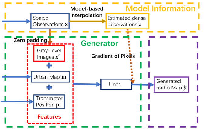
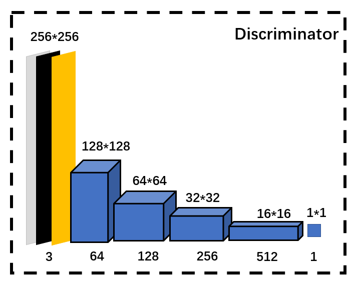
In this section, we present the design of the proposed RME-GAN, with the overall structure shown as Fig. 3. We first introduce the basic sketch of RME-GAN in Section IV-A, before describing the two-phase customization of features and loss functions in Section IV-B and Section IV-C, respectively.

(a) Structure of Generator

(b) Structure of Discriminator

Figure 3: Structure of RME-GAN: a) The generator takes input $\mathcal{F}_{i}$ and consider the model information during training, where two phases of loss functions are applied to train the generator; b) The discriminator consists of 4 layers and generates a one-dimensional probability output. The discriminator input consists of 3 channels: the generated/true radio map (marked as orange), and the prior information as two-channel one-hot encodings (marked as grey and black).

TABLE I: Structure of Unet

Layer	Input	1	2	3	4	5	6	7	8	9
Resolution	256	256	128	64	64	32	32	16	8	4
Channel	3	6	40	50	60	100	100	150	300	500
Filter	3	5	5	5	5	3	5	5	5	4
Layer	10	11	12	13	14	15	16	17	18	Output
Resolution	8	16	32	32	64	64	128	256	256	256
Channel	300+300	150+150	100+100	100+100	60+60	50+50	40+40	20+6+3	20+3	1
Filter	4	4	3	6	5	6	6	5	5	-

IV-A Sketch of RME-GAN

RME-GAN learns a mapping function $g(\cdot)$ from the region features $\mathcal{F}_{i}$ to its output estimated full radio map $\tilde{\mathbf{y}}_{i}$. Since it is also a one-to-one mapping problem, we could design RME-GAN based on the general cGAN structure similar to Fig. 2. More specifically, we utilize an 18-layer deep Unet [8] structure for the sketch of the generator, with parameters shown in Table. I.

To reformat the input features in $\mathcal{F}_{i}$, we first interpolate the sparse observations $(\mathbf{x}_{i},\mathbf{c}_{i})$ to the same size as region size via zero padding, i.e., $\mathbf{x}_{i}^{\prime}\in\mathbb{R}_{+}^{256\times 256}$. Since we consider a convolutional neural network (CNN) structure for Unet, the interpolated zero would not influence other features. We then encode the transmitter locations $\mathbf{P_{t}}_{i}$ also in a $256\times 256$ matrix $\mathbf{p}_{i}$, where the transmitter positions in $\mathbf{p}_{i}$ are marked as $1$ and other positions are $0$. Features $\mathcal{F}_{i}$ are encoded to three channels of features with size $256\times 256$, i.e., $\mathbf{f}_{i}=\{\mathbf{x}_{i}^{\prime},\mathbf{m}_{i},\mathbf{p}_{i}\}$.

With the encoded features, the basic objective function of RME-GAN can be designed by

$$\min_{G}\max_{D}\quad V(D,G)=\mathbb{E}_{y,I\sim p_{\rm data}(\bf{y},\bf{I})}[\log D(\bf{y,I})]+$$

$$\mathbb{E}_{f\sim p_{\rm data}(\bf{f})}[\log(1-D(G(\bf{f}),\mathbf{I}))],$$ (7)

where $p_{\rm data}(\bf{y,I})$ is the joint distribution with the prior knowledge $\mathbf{I}$. More specifically, $\mathbf{I}$ can be designed as a function of the region features, i.e., $\mathbf{I}=f(\mathcal{F}_{i})$ or some determined labels, such as fake or real [35]. Here, we set $\mathbf{I}\in\mathbb{R}^{256\times 256\times 2}$ to represent the one-hot encodings in two-channel to give prior information to the discriminator as the input is a generated or real radio map.

We can split the min-max optimization problem to sub-problems, and train the generator $G$ and discriminator $D$ iteratively. Specifically, the loss function to optimize $D$ is

$$L_{D}=-V(D,G),$$ (8)

and the general loss function to optimize $G$ is

$$L_{G}=\mathbb{E}_{x\sim p_{\rm data}(\bf{x})}[\log(1-D(G(\bf{x}),\mathbf{I}))].$$ (9)

The overall sketch of RME-GAN is illusrated in Fig. 3. Note that the cGAN can be customized by adding additional loss terms to capture desired properties. In this work, we consider a two-phase loss function design for Eq. (9) to capture the global and local information, respectively. More details will be discussed in Section IV-B and IV-C.

IV-B Two-phase Customization in RME-GAN

Earlier, we have identified two challenges in radio map estimation: 1) how to efficiently integrate radio propagation model with learning machines to capture global information; and 2) how to estimate the details from biased and non-uniformly distributed observations. The first challenge lies in the estimation of global model information while the second challenge deals with shadowing effect and obstacle impact. To handle these challenges, we utilize different sampling strategies to extract global patterns and local features, respectively, as follows.

IV-B1 Upsampling for global information

In general, radio propagation should follow certain pathloss models, such as LDPL [4]. Thus, to model global pathloss, we first upsample the sparse observations $(\mathbf{x}_{i},\mathbf{c}_{i})$ to a radio map template $\mathbf{z}\in\mathbb{R}_{+}^{256\times 256}$ via model-based interpolation (MBI). Suppose that a system has $N_{t}$ transmitter with positions $(a_{k},b_{k})$, $1\leq k\leq N_{t}$. In MBI, the signal strength (in dB) at position $(a,b)$ can be modeled as

$$P(a,b)=\sum_{k=1}^{N_{t}}(\alpha_{k}-10\theta_{k}\log_{10}(\sqrt{(a_{k}-a)^{2}+(b_{k}-b)^{2}})),$$ (10)

where $\alpha_{k}$ is the power from $k$th transmitter at the reference distance. Then, we optimize the paramters of the LDPL model from the observations by

$$\min_{\alpha_{k},\theta_{k}}\sum_{j=1}^{K_{i}}(\mathbf{x}(j)-P(\mathbf{c}(j)))^{2}$$ (11)

where $\mathbf{x}(j)$ is the $j$th observation with position $\mathbf{c}(j)$. By apply the LDPL model with estimated parameters, we can upsample the sparse observations $\mathbf{x}_{i}$ as $\mathbf{z}_{i}\in\mathbb{R}_{+}^{256\times 256}$.

Although MBI may be not able to capture full effect of obstacles and shadowing, upsampled template can still capture the global propagation pattern together with MBI model parameters. Consideration of upsampled features during the training process can provide a general guideline on radio map reconstruction. We introduce how to use $\mathbf{z}_{i}$ to design loss functions of Phase 1 in Section IV-C.

IV-B2 Downsampling for detailed features

After estimating a template of reconstructed radio maps, we downsample the sparse observations in the second phase to correct errors in the details. We consider two downsampling strategies:

• Geometry-wise downsampling: As discussed in Section III, sparse observations may be non-uniformly distributed over the whole space. To deal with unevenly distributed samples, we apply geometric information to downsample the observations. To balance the sample numbers in different locations, we first build superpixels [38] based on urban map or interpolated template to split the entire region into $N_{s}$ pieces. In each piece, we only pick one observation of peak energy. Then, we have a downsampled version of observations $\mathbf{x}\in\mathbb{R}_{+}^{K}$ as $\mathbf{x_{s}}\in\mathbb{R}_{+}^{N_{s}}$. In addition to superpixel-based space cut, other methods such as Voronoi diagram [4] or spectral clustering [39] can be also applied.

• Frequency-wise downsampling: In digital signal processing, details and outliers are related to high frequencies in Fourier space. Thus, we could also transform the estimated radio map $\tilde{\mathbf{y}}$ to Fourier space as $\hat{\mathbf{y}}$. Then, we can select the first $N_{f}$ Fourier coefficients in the high frequency part as additional information in loss functions of the second phase, i.e., $\hat{\mathbf{y}}_{f}\in\mathbb{R}^{N_{f}}$.

With the extracted features under different sampling strategies, we propose a two-phase design on the loss functions for the training of the generator, i.e.,

$$L_{G}^{\prime}=\left\{\begin{aligned} &L_{G}+L_{Global}\quad&\text{if}\quad\epsilon<\tau\\ &L_{G}+L_{Local}\quad&\text{if}\quad\epsilon\geq\tau\end{aligned}\right.,$$ (12)

where $L_{Global}$ consist of loss functions favoring global model information and $L_{Local}$ are the loss functions focusing on the local details. Here, a decision variable $\epsilon$ can be designed according to certain criteria, i.e., length of epochs or validation accuracy. For convenience, we keep a validation data set to evaluate the validation accuracy at each epoch to determine the phase change point. The specific design of loss functions will be introduced next in Section IV-C.

IV-C Loss Functions

After introducing the overall frameworks, we now present the design of loss functions.

IV-C1 Phase 1 - Global Model Prediction

We first introduce the design of loss function in the first phase.

• Baseline loss function: The first term is the mean squared error (MSE) between the generated radio map and the ground truth $\mathbf{y}$:

  $$L_{\rm MSE}=\frac{1}{256\times 256}\cdot||\mathbf{y}-\tilde{\mathbf{y}}||_{F}^{2},$$ (13)

  where $||\cdot||_{F}$ is the Frobenius norm and $\tilde{\mathbf{y}}=g(\mathbf{f})$. We also consider a second term to be the total variation which describes the smoothness of the generated radio map [35]. More specifically, we apply the total variation of images

  $$L_{\rm TV}=\sum_{i,j\in\mathcal{N}}||\tilde{\mathbf{y}}(i)-\tilde{\mathbf{y}}(j)||_{2}^{2},$$ (14)

  where $\mathcal{N}$ indicates pixel neighborhood and $\tilde{\mathbf{y}}(i)$ is the $i$th element of the estimated radio map $\tilde{\mathbf{y}}$.

• Loss function of global information: In addition to the baseline loss functions, we also utilize upsampled radio map $\mathbf{z}$ from MBI to help the learning of global radio propagation patterns. Instead of directly evaluating the difference between $\tilde{\mathbf{y}}$ and $\mathbf{z}$, we focus on gradient patterns. Such gradient patterns feature smoothness of radio propagation from transmitters to the surroundings. Since the first phase aims to learn the radio propagation model, MBI can help RME-GAN to learn the propagation model and speed up training. To obtain the gradient-based loss function, we first calculate the gradient of each pixel in the radio map for up, down, right and left, i.e.,

  $$\mathcal{G}(\tilde{\mathbf{y}}(i))=[\mathcal{G}_{\rm up},\mathcal{G}_{\rm down},\mathcal{G}_{\rm right},\mathcal{G}_{\rm left}]\in\mathbb{R}^{4}.$$ (15)

  Then, we calculate the cosine similar between $\mathcal{G}(\tilde{\mathbf{y}}(i))$ and $\mathcal{G}({\mathbf{z}}(i))$. Then, the loss function of global information is defined as

  $$L_{\rm Gradient}=\sum_{i=1}^{256\times 256}CS(\mathcal{G}(\tilde{\mathbf{y}}(i)),\mathcal{G}({\mathbf{z}}(i))),$$ (16)

  where $CS(\cdot)$ refers to the cosine similarity [40].

IV-C2 Phase 2 - Local Shadowing Estimation

Next, we introduce the loss functions for local features in the second phase.

• Baseline loss function: Similar to the first phase, the generated radio map should be smooth over the entire space. Thus, we also use total variation $L_{\rm TV}$ as one of the baseline loss functions. In addition, the $L_{\rm MSE}$ is also used here to control the overall accuracy. However, to emphasize more details depending on the downsampled observations, we assign a much smaller weight on $L_{\rm MSE}$ in the second phase compared to the first phase.

• Geometric loss function: To mitigate the effect of non-uniformly distributed observations, we favor downsampled observations among all observations. Since the sparse observations are also true power gain in the radio map, we define a geometric loss function as the MSE between downsampled $\mathbf{x}_{s}=\mathbf{y}_{s}$ and the generated PSD at the same positions, denoted by $\tilde{\mathbf{y}}_{s}$, i.e.,

  $$L_{\rm Geo}=MSE(\mathbf{x}_{s},\tilde{\mathbf{y}}_{s}).$$ (17)

• Frequency domain loss function: As discussed before in Section IV-B, high frequency coefficients in the Fourier space can capture the details or outliers in a radio map. To capture such information, we also calculate the MSE between $\hat{\mathbf{y}}_{f}$ and $\hat{\tilde{\mathbf{y}}}_{f}$ denoted by

  $$L_{\rm HPF}=MSE(\hat{\mathbf{y}}_{f},\hat{\tilde{\mathbf{y}}}_{f}),$$ (18)

  where $\hat{\mathbf{y}}_{f}$ includes the first top $N_{f}$ high frequency coefficients in the Fourier domain.

• Multi-scale structural similarity index: In image processing, multi-scale structural similarity index (MS-SSIM) is a useful term to evaluate the image quality based on human visual system [41]. Since details in radio map can be viewed as a fine-resolution image while the model-based template can be viewed as a coarse-resolution image, we could also consider the MS-SSIM index to improve the quality of generated radio map in the second phase. Let $\mathbf{u}={u_{i}|i=1,2,\cdots,N}$ and $\mathbf{v}={v_{i}|i=1,2,\cdots,N}$ be two discrete non-negative signals, e.g., two image patches from the same position or two radio map residing on the same region. The luminance, contrast and structure comparison measurements can be calculated as follows:

  $$l(\mathbf{u},\mathbf{v})=\frac{2\mu_{u}\mu_{v}+C_{1}}{\mu_{u}^{2}+\mu_{v}^{2}+C_{1}},$$ (19)

  $$c(\mathbf{u},\mathbf{v})=\frac{2\sigma_{u}\sigma_{v}+C_{2}}{\sigma_{u}^{2}+\sigma_{v}^{2}+C_{2}},$$ (20)

  $$s(\mathbf{u},\mathbf{v})=\frac{2\sigma_{uv}+C_{3}}{\sigma_{u}\sigma_{v}+C_{3}},$$ (21)

  where $\mu$ represents mean, $\sigma$ is the variance, $C_{i}$ are small constants introduced in [42]. To calculate MS-SSIM, the system iteratively applies a low-pass filter and downsamples the filtered image by a factor of 2 on reference and distorted image signals as inputs. Suppose that $M$ is the highest scale. The overall MS-SSIM is calculated by

  $${\rm SSIM}(\mathbf{u},\mathbf{v})=[l_{M}(\mathbf{u},\mathbf{v})]^{\alpha_{M}}\cdot\prod_{j=1}^{M}[c_{j}(\mathbf{u},\mathbf{v})]^{\beta_{j}}[s_{j}(\mathbf{u},\mathbf{v})]^{\gamma_{j}}.$$ (22)

  Here, ${\rm SSIM}(\mathbf{u},\mathbf{v})\leq 1$, and ${\rm SSIM}(\mathbf{u},\mathbf{v})=1$ iff $\mathbf{u}=\mathbf{v}$. The MS-SSIM loss function is defined by

  $$L_{\rm SSIM}=1-{\rm SSIM}(\mathbf{y},\tilde{\mathbf{y}}).$$ (23)

  More properties of MS-SSIM can be found in [41].

IV-D Summary of Two-Phase Training Strategy

Combining all the loss terms aforementioned, the final loss function to train the generator is represented as

$$L_{G}^{\prime}=\left\{\begin{aligned} &\lambda_{1}L_{G}+\lambda_{2}L_{\rm MSE}+\lambda_{3}L_{\rm TV}+\lambda_{4}L_{\rm Gradient},&\epsilon<\tau\\ &\lambda_{1}L_{G}+\lambda_{2}L_{\rm MSE}+\lambda_{3}L_{\rm TV}+\\ &\lambda_{5}L_{\rm SSIM}+\lambda_{6}L_{\rm Geo}+\lambda_{7}L_{\rm HPF}&\epsilon\geq\tau\end{aligned}\right.$$

where $\lambda_{i}$ are the weights to control each loss term. In the first phase, we aims to apply model-based interpolation to help RME-GAN learn a template to capture the radio propagation model. After enough epochs, we favor more on the local information to correct errors in the details on the template by learning the shadowing effect and obstacle impact. Although some baseline loss functions are shared in both phases, the weights can be different depending on the specific tasks.

V Experimental Results

In this section, we present the experimental results of the proposed methods.

V-A Experiment Setup

(a) Example of Urban Images.

(b) Example of Radio Map

Figure 4: Examples of RadioMapSeer Dataset: a) Urban maps with buildings as white and background as black; b) radio map with pathloss as yellow.

(a) Ground Truth

(b) Three Selected Regions

Figure 5: One Example of Radio Map

V-A1 Dataset

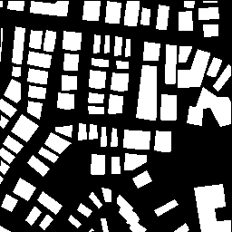
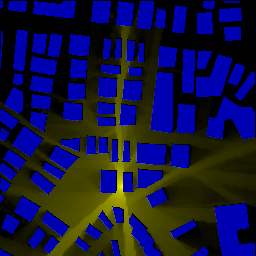
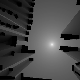
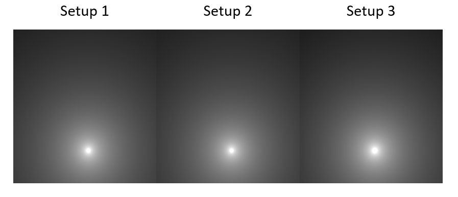
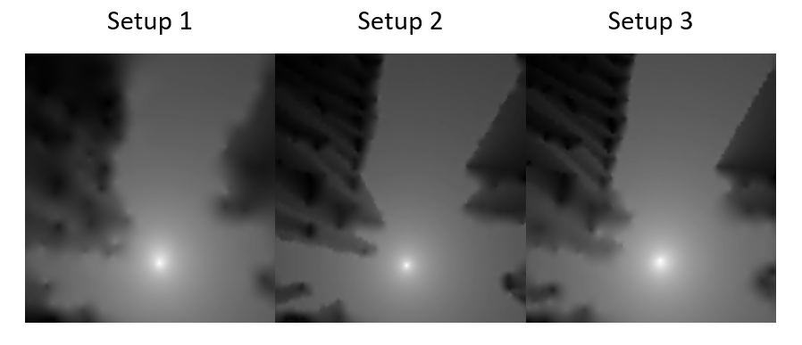
In this work, we test the performance of the proposed method in the RadioMapSeer dataset [8]. The RadioMapSeer dataset consists of 700 maps with 80 transmitter locations per map. The city maps are taken from OpenStreetMap [43] covering metropolitans such as Ankara, Berlin, Glasgow, Ljubljana, London and Tel Aviv. The heights of the transmitters, receivers and buildings are set to 1.5m, 1.5m, and 25m, respectively, in this dataset. The transmitter power equals 23dBM and the carrier frequency is 5.9GHz. The radio maps are generated using the software WinProp [44], and are saved in a 2D grid of $256\times 256m^{2}$. The radio map has a 1-meter resolution. More specifically, we test on the higher accuracy simulations in the RadioMapSeer datasets. An example of the RadioMapSeer dataset is shown in Fig. 4, where building segmentation are consider as the urban map in our framework. The sparse observations are sampled from each radio map for training and testing.

(a) NMSE

(b) RMSE

Figure 6: Performance of Different Methods over Different Ratio of Observations.

V-A2 Data Splitting

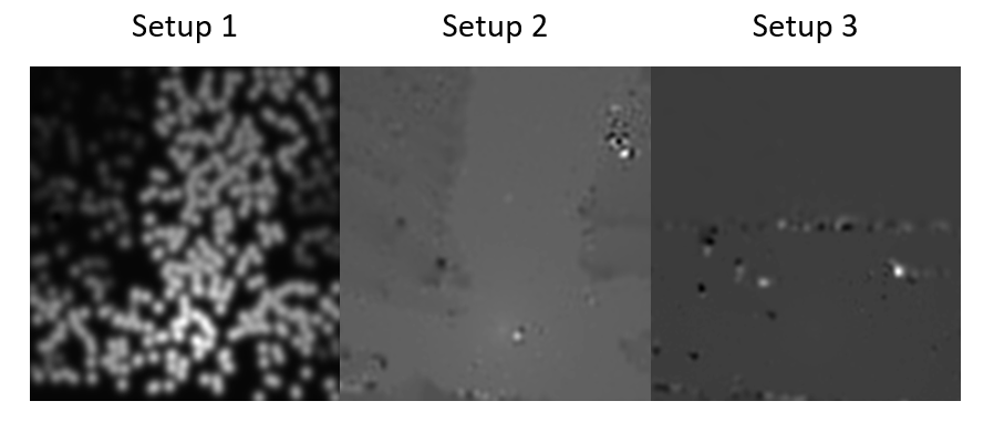
As mentioned in Section III, the sparse observations can be either uniformly or non-uniformly distributed over the whole space, and different regions may have different number of observations. Thus, we sample the sparse observations under three different scenarios:

• Setup 1 (Uniformly distributed): We uniformly sample $1\%$ of sparse observations from the whole radio map.

• Setup 2 (Unbalanced sample distribution among regions): In this setup, we sample the radio map at a random ratio from $1\%\sim 10\%$ in each region, and the sparse observations are uniformly distributed.

• Setup 3: (Non-uniformly distributed) We divide the radio map into two sides randomly. Then, we sample $1\%$ of observations from one side and $10\%$ from the other side.

We compare the proposed RME-GAN with other methods in all the three scenarios to demonstrate its efficacy. The whole dataset consists of 700 regions. For each experiment scenario, we split the dataset with 500 regions as training data, 100 regions for testing, and 100 regions for validation.

TABLE II: Performance in Different Setups

	Setup 1		Setup 2		Setup 3
Model	NMSE	RMSE	NMSE	RMSE	NMSE	RMSE
Kriging	0.8863	0.1947	0.8987	0.1962	0.9118	0.1971
RBF	0.3532	0.1343	0.1830	0.0884	0.3215	0.1295
MBI	0.8837	0.1973	0.5158	0.1499	0.5174	0.1500
cGAN	0.1559	0.0904	0.15077	0.0888	0.1506	0.0889
AE	0.1823	0.0978	0.2885	0.1238	0.2783	0.1217
Deep AE	0.1898	0.0998	0.3152	0.1295	0.3058	0.1274
Unet	0.0093	0.0220	0.0053	0.0166	0.0050	0.0161
RadioUnet	0.0052	0.0164	0.0042	0.0148	0.0046	0.0155
RME-GAN	0.0043	0.0151	0.0036	0.0130	0.0038	0.0140

(a) RME-GAN

(b) RadioUnet

(c) MBI

(d) Kriging

(e) RBF

(f) AE

Figure 7: Visualization Results of Different Methods

V-A3 Parameters of Learning Models

We utilize an 18-layer Unet for the generator with parameters shown in Table. I, and a 4-layer discriminator shown as Fig. 3(b). In the first phase, the weights of each loss term are set as $\lambda_{2}=10$, $\lambda_{3}=0.01$, $\lambda_{4}=1$. In the second phase, we set the weights as $\lambda_{1}=10$, $\lambda_{2}=1$, $\lambda_{3}=0.001$, $\lambda_{4}=0.0001$, $\lambda_{5}=0.0001$ and $\lambda_{6}=0.0001$. Note that, although both phases contains the $L_{\rm MSE}$, $\lambda_{2}$ is set to be smaller in the second phase since we favor the downsampled radio map for detail correction.

V-B Overall Accuracy

We first present the results in different setups. To evaluate the performance of the proposed RME-GAN, we compare with the MBI interpolation [4], RBF interpolation [6], radioUnet [8], auto-encoder (AE) [10], deep AE [10], traditional Unet, Kriging interpolation [17], and traditional cGAN [33]. The Normalized Mean Square Error (NMSE) and Root Mean Square Error (RMSE) of the reconstructed radio map are present in Table II.

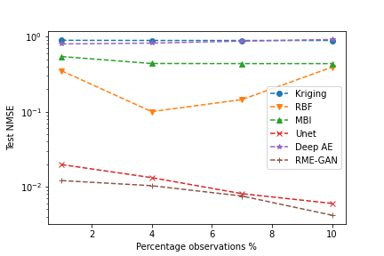
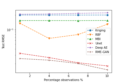
In Setup 1, samples are uniformly distributed. The learning-based approaches have better performance than the model-based and interpolation-based methods since the environment of these regions are more complex and the radio map is sensitive to shadowing effect. Our RME-GAN outperforms all the methods in Setup 1. Especially in comparison with traditional cGAN, our two-phase training process provides more information and display superior performance. We also compare different methods over different ratio of observations in Setup 1, shown in Fig. 6. Our proposed RME-GAN has the best performance results, as Table II further illustrates.

In Setup 2 and Setup 3, observations are biased among different regions and non-uniformly distributed, respectively. RME-GAN still shows the best results owing to the design of different sampling strategies. The experimental results demonstrate the power of the proposed resampling methods and RME-GAN in radio map reconstruction.

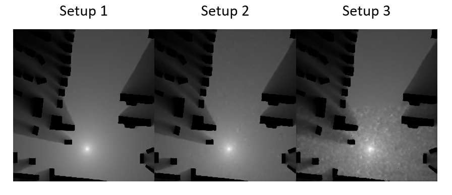
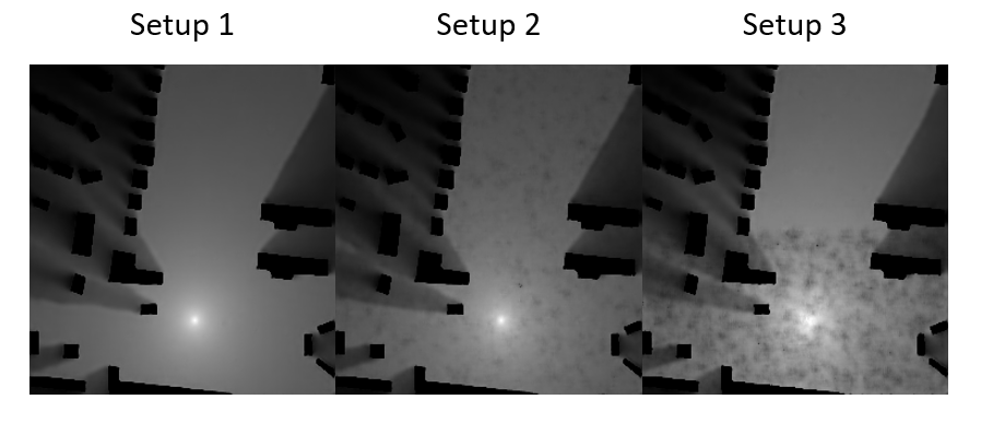
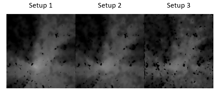
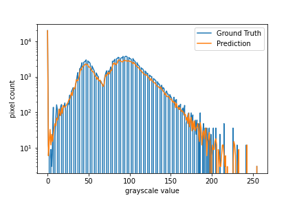
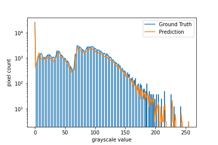
Beyond the numerical results obtained, we also present the visualization results of a radio map in Fig. 5(a). The reconstructed results from different methods are shown in Fig. 7. Since interpolation-based methods, such as MBI and RBF cannot capture the impact of environment efficiently, it fails to reconstruct the radio map in both three setups. Kriging-based methods provide a blurred construction of radio map as it estimates PSD from neighborhood data. Learning-based methods generally display better reconstruction. Compared to RadioUnet and AE, our RME-GAN constructs more accurate radio maps. Especially in view of Setup 3 where the sparse observations are non-uniformly distributed over the region, the proposed RME-GAN outperforms other existing learning methods. This happens because our resampling strategy is able to balance the samples over different locations. We also display the histogram of the reconstructed radio map in Setup 1 from RME-GAN as shown in Fig. 8, where RME-GAN is able to capture the distribution of PSD.

(a) Histogram in a training sample

(b) Histogram in a test sample

Figure 8: One Example of Histograms of PSD in Reconstructed Radio Maps

Figure 9: Validation Performance over Different Phase

V-C Robustness

V-C1 Two-Phase Training

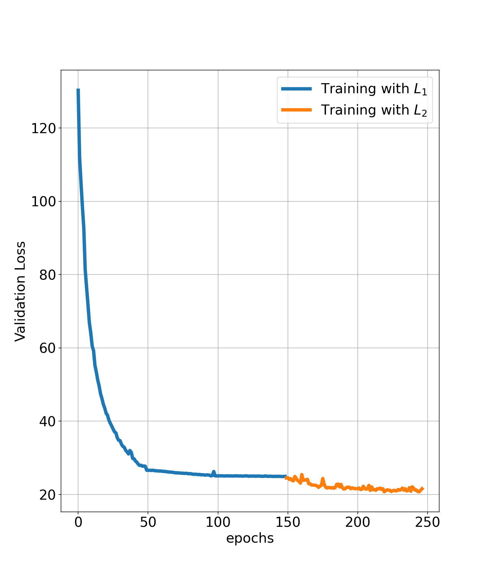
We first confirm the robustness of the two-phase training strategies. The validation error over time is shown in Fig. 9. From the results, the error drops when the training moves from phase 1 to phase 2, which indicates that the second phase could better correct detailed errors for the propagation template model from the first phase by leveraging the shadowing information.

V-C2 Zero-shot Learning

Zero-shot learning concerns the recognition of new concepts or new scenarios when a learning model is trained with generic datasets [45]. To evaluate the robustness and generalization of the proposed RME-GAN, we train the generator model by using data from Setup 1, but we test the performance in the data from Setup 2 and 3, respectively. The results are shown in Table III. From the results, we see that our RME-GAN can still obtain a superior performance in the test dataset with different distributions while other learning-based methods all observe a significant performance drop.

TABLE III: Performance of Zero-shot Learning

Model	Setup 2		Setup 3
	NMSE	RMSE	NMSE	RMSE
cGAN	0.1613	0.0918	0.1984	0.1018
AE	0.2051	0.1038	0.2259	0.1094
Deep AE	0.1870	0.0991	0.1981	0.1019
Unet	0.0082	0.0208	0.0254	0.0367
RadioUnet	0.0052	0.0165	0.0148	0.0280
RME-GAN	0.0042	0.0150	0.0067	0.0190

TABLE IV: Performance in Selected Areas

Model	Red Area		Green Area		Blue Area
	RMSE	NMSE	RMSE	NMSE	RMSE	NMSE
RBF	0.0574	0.2794	0.0929	0.3317	0.0868	0.2803
Kriging	0.0675	0.3867	0.0890	0.3041	0.0819	0.2491
AE	0.0545	0.2518	0.0831	0.2651	0.0711	0.1879
MBI	0.1087	0.9520	0.1368	0.7183	0.0952	0.3372
cGAN	0.0449	0.1714	0.0723	0.2009	0.0466	0.0807
RadioUnet	0.0164	0.0228	0.0250	0.0240	0.0210	0.0163
RME-GAN	0.0151	0.0190	0.0221	0.0189	0.0172	0.0110

TABLE V: Outage Evaluation (Prediction Error)

Model	Threshod = 5		Threshod = 25
	Samples = 1	Average	Samples = 1	Average
RBF	0.1165	0.1265	0.2303	0.2349
MBI	0.1169	0.1391	0.1599	0.2359
Kriging	0.1870	0.0991	0.1381	0.1520
AE	0.1168	0.1525	0.1498	0.1586
RadioUnet	0.0085	0.0122	0.0144	0.0158
RME-GAN	0.0074	0.0105	0.0120	0.0141

V-C3 Performance in Areas with Lower Energy

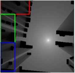
Compared to the areas with larger energy, the areas with lower power spectrum are more sensitive to the environment. To validate the performance of RME-GAN in areas with lower power, we select three areas shown as Fig. 5(b) and test different methods in these three regions. The performance is shown in Table IV, where RME-GAN outperforms other methods in all areas and display more robustness in the low-power areas.

V-D Outage Fault Diagnosis

We perform outage analysis as a fault diagnosis. In some realistic applications, e.g. outage detection, we usually only need a coarse resolution of radio map instead of the fine-resolution one. To evaluate the power of the proposed RME-GAN in reconstructing radio maps for such applications, we also compare the accuracy of the reconstructed outage maps. In our definition, a location experiences power outage if its PSD falls below a preset threshold. Then, we can segment the radio map into an outage map with normal and outage areas, i.e., a binary segmentation. We compare the outage maps for all methods against two exemplary thresholds, i.e., 5 and 25. We measure performance by using segmentation errors in Table V. Moreover, we present the results of one randomly selected regions, and the average of 10 randomly selected regions. Our proposed RME-GAN provides a more accurate outage map reconstruction compared to other approaches, which demonstrates the practicability of RME-GAN in network fault detection applications.

VI Conclusions

In this work, we propose a two-phase learning frameworks (RME-GAN) for radio map estimation from sparse RF measurements. Our RME-GAN first estimates a template to capture the global radio propagation patterns based model-based interpolation. In the second phase it learns the shadowing effects via geometric and frequency downsampling. The experimental results demonstrate the performance advantages and the robustness of the proposed RME-GAN, together with the two-phase training strategies in radio map estimation.

The rapid growth and expansion of IoT and 5G systems make efficient estimation and utilization of radio map become increasingly important. Radiomap estimation are important tools for resource allocation and network planning. One promising future direction may be fault diagnosis based on the sparse RF observations from deployed sensors or reports from a few users. Another fruitful direction would be the integration of model-based approaches with learning machines. Our future works plan to consider these and other related directions.

References

- [1] Y. Deng et al., “Radio environment map construction using super-resolution imaging for intelligent transportation systems,” in IEEE Access, vol. 8, pp. 47272-47281, Mar. 2020.
- [2] S. Bi, J. Lyu, Z. Ding and R. Zhang, “Engineering radio maps for wireless resource management,” in IEEE Wireless Communications, vol. 26, no. 2, pp. 133-141, Apr. 2019.
- [3] S. Debroy, S. Bhattacharjee and M. Chatterjee, “Spectrum map and its application in resource management in cognitive radio networks,” in IEEE Transactions on Cognitive Communications and Networking, vol. 1, no. 4, pp. 406-419, Dec. 2015.
- [4] M. Lee and D. Han, “Voronoi tessellation based interpolation method for wi-fi radio map construction,” in IEEE Communications Letters, vol. 16, no. 3, pp. 404-407, Mar. 2012.
- [5] J. A. Bazerque, G. Mateos and G. B. Giannakis, “Group-lasso on splines for spectrum cartography,” in IEEE Transactions on Signal Processing, vol. 59, no. 10, pp. 4648-4663, Oct. 2011.
- [6] J. Krumm and J. Platt, “Minimizing calibration effort for an indoor 802.11 device location measurement system,”, Microsoft Research, Nov. 2003.
- [7] S. Kuo and Y. Tseng, “Discriminant minimization search for largescale rf-based localization systems,” in IEEE Transactions on Mobile Computing, vol. 10, no. 2, pp. 291-304, Feb. 2011.
- [8] R. Levie, Ç. Yapar, G. Kutyniok and G. Caire, “Radiounet: fast radio map estimation with convolutional neural networks,” in IEEE Transactions on Wireless Communications, vol. 20, no. 6, pp. 4001-4015, Jun. 2021
- [9] O. Ronneberger, P. Fischer, and T. Brox, “U-net: convolutional networks for biomedical image segmentation,” in International Conference on Medical image computing and computer-assisted intervention, Munich, Germany, Nov. 2015, pp. 234-241.
- [10] Y. Teganya and D. Romero, “Deep completion autoencoders for radio map estimation,” in IEEE Transactions on Wireless Communications, vol. 21, no. 3, pp. 1710-1724, Mar. 2022.
- [11] S. C. Beck, J. L. Turner, and O. Kovo, “High-resolution radio maps of wolf-rayet galaxies: optically thick h ii regions?.” The Astronomical Journal, vol. 120, no. 1, pp. 244, 2000.
- [12] O. Esrafilian and D. Gesbert, “3d city map reconstruction from uav-based radio measurements,” GLOBECOM 2017, Singapore, Dec. 2017, pp. 1-6.
- [13] J. Johansson, W. A. Hapsari, S. Kelley and G. Bodog, “Minimization of drive tests in 3GPP release 11,” in IEEE Communications Magazine, vol. 50, no. 11, pp. 36-43, Nov. 2012.
- [14] M. Mirza, and S. Osindero,“Conditional generative adversarial nets,” arXiv preprint arXiv:1411.1784, 2014.
- [15] X. Fu, N. D. Sidiropoulos, J. H. Tranter and W. K. Ma, “A factor analysis framework for power spectra separation and multiple emitter localization,” in IEEE Transactions on Signal Processing, vol. 63, no. 24, pp. 6581-6594, Dec.15, 2015.
- [16] H. Braham, S. B. Jemaa, G. Fort, E. Moulines and B. Sayrac, “Fixed rank kriging for cellular coverage analysis,” in IEEE Transactions on Vehicular Technology, vol. 66, no. 5, pp. 4212-4222, May 2017.
- [17] G. Boccolini, G. Hernández-Peñaloza and B. Beferull-Lozano, “Wireless sensor network for Spectrum Cartography based on Kriging interpolation,” 2012 IEEE 23rd International Symposium on Personal, Indoor and Mobile Radio Communications - (PIMRC), Sydney, NSW, Australia, Sep. 2012, pp. 1565-1570.
- [18] A. E. C. Redondi, “Radio map interpolation using graph signal processing,” in IEEE Comm. Letters, vol. 22, no. 1, pp. 153-156, Jan. 2018.
- [19] X. Du, X. Liao, M. Liu and Z. Gao, “CRCLoc: a crowdsourcing-based radio map construction method for wifi fingerprinting localization,” in IEEE Internet of Things Journal, vol. 9, no. 14, pp. 12364-12377, Jul. 2022.
- [20] S. Zhang, T. Yu, J. Tivald, B. Choi, F. Ouyang, and Z. Ding, “Exemplar-based radio map reconstruction of missing areas using propagation priority,” arXiv preprint arXiv:2209.04566, 2022.
- [21] M. S. Riaz, H. N. Qureshi, U. Masood, A. Rizwan, A. Abu-Dayya and A. Imran, “Deep learning-based framework for multi-fault diagnosis in self-healing cellular networks,” 2022 IEEE Wireless Communications and Networking Conference (WCNC), Austin, TX, USA, Apr. 2022, pp. 746-751.
- [22] D. Schäufele, R. L. G. Cavalcante and S. Stanczak, “Tensor completion for radio map reconstruction using low rank and smoothness,” 2019 IEEE 20th International Workshop on Signal Processing Advances in Wireless Communications (SPAWC), Cannes, France, Jul. 2019, pp. 1-5.
- [23] C. Parera, Q. Liao, I. Malanchini, C. Tatino, A. E. C. Redondi and M. Cesana, “Transfer learning for tilt-dependent radio map prediction,” in IEEE Transactions on Cognitive Communications and Networking, vol. 6, no. 2, pp. 829-843, Jun. 2020.
- [24] S. K. Vankayala, S. Kumar, I. Roy, D. Thirumulanathan, S. Yoon and I. S. Kanakaraj, “Radio map estimation using a generative adversarial network and related business aspects,” 2021 24th International Symposium on Wireless Personal Multimedia Communications (WPMC), Okayama, Japan, Feb. 2021, pp. 1-6.
- [25] Chun-Hao Liu, Hun Chang, Taesuh Park; Proceedings of the IEEE/CVF Conference on Computer Vision and Pattern Recognition (CVPR) Workshops, 2020, pp. 498-499.
- [26] H. Zou et al., “Adversarial learning-enabled automatic wifi indoor radio map construction and adaptation with mobile robot,” in IEEE Internet of Things Journal, vol. 7, no. 8, pp. 6946-6954, Aug. 2020.
- [27] X. Wang, X. Wang, S. Mao, J. Zhang, S. C. G. Periaswamy and J. Patton, “Indoor radio map construction and localization with deep gaussian processes,” in IEEE Internet of Things Journal, vol. 7, no. 11, pp. 11238-11249, Nov. 2020.
- [28] Y. Zeng, X. Xu, S. Jin and R. Zhang, “Simultaneous navigation and radio mapping for cellular-connected uav with deep reinforcement learning,” in IEEE Transactions on Wireless Communications, vol. 20, no. 7, pp. 4205-4220, Jul. 2021.
- [29] K. Suto, S. Bannai, K. Sato, K. Inage, K. Adachi and T. Fujii, “Image-driven spatial interpolation With deep learning for radio map construction,” in IEEE Wireless Communications Letters, vol. 10, no. 6.
- [30] H. J. Bae and L. Choi, ”Large-scale indoor positioning using geomagnetic field with deep neural networks,” 2019 IEEE International Conference on Communications (ICC), Shanghai, China, May 2019, pp. 1-6.
- [31] T. Imai, K. Kitao and M. Inomata, “Radio propagation prediction model using Cconvolutional neural networks by deep learning,” 2019 13th European Conference on Antennas and Propagation (EuCAP), Krakow, Poland, Jun. 2019, pp. 1-5.
- [32] D. Romero and S. J. Kim, “Radio map estimation: a data-driven approach to spectrum cartography,” in IEEE Signal Processing Magazine, vol. 39, no. 6, pp. 53-72, Nov. 2022.
- [33] I. Goodfellow, J. Pouget-Abadie, M. Mirza, B. Xu, D. Warde-Farley, S. Ozair, A. Courville, and Y. Bengio. “Generative adversarial networks,” Communications of the ACM, vol. 63, pp. 139-144, Nov. 2020.
- [34] D. Pathak, P. Krahenbuhl, J. Donahue, T. Darrell, and A. A. Efros, “Context encoders: Feature learning by inpainting,” Proceedings of the IEEE Conference on Computer Vision and Pattern Recognition, Las Vegas, Nevada, USA, 2016, pp. 2536-2544.
- [35] Y. Liu, Z. Qin, T. Wan, and Z. Luo, “Auto-painter: cartoon image generation from sketch by using conditional Wasserstein generative adversarial networks,” Neurocomputing, vol. 311, pp. 78-87, Oct. 2018.
- [36] P. Isola, J. Y. Zhu, T. Zhou, and A. A. Efros, “Image-to-image translation with conditional adversarial networks, in Proceedings of the IEEE Conference on Computer Vision and Pattern Recognition Honolulu, Hawaii, USA, 2017, pp. 1125-1134.
- [37] T. C. Wang, M. Y. Liu, J. Y. Zhu, A. Tao, J. Kautz, and B. Catanzaro, “High-resolution image synthesis and semantic manipulation with conditional gans,” in Proceedings of the IEEE Conference on Computer Vision and Pattern Recognition, Salt Lake City, Utah, USA, 2018, pp. 8798-8807.
- [38] S. Zhang, Q. Deng, and Z. Ding,“Multilayer graph spectral analysis for hyperspectral images,” EURASIP Journal on Advances in Signal Processing, vol. 1, no. 92 pp. 1-25, 2022.
- [39] S. Zhang, Z. Ding and S. Cui, “Introducing hypergraph signal processing: theoretical foundation and practical applications,” in IEEE Internet of Things Journal, vol. 7, no. 1, pp. 639-660, Jan. 2020.
- [40] H. V. Nguyen, and L. Bai, “Cosine similarity metric learning for face verification,” in Asian Conference on Computer Vision, Berlin, Heidelberg, 2010, pp. 709-720.
- [41] Z. Wang, E. P. Simoncelli and A. C. Bovik, “Multiscale structural similarity for image quality assessment,” the Thrity-Seventh Asilomar Conference on Signals, Systems and Computers, Pacific Grove, CA, USA, 2003, pp. 1398-1402.
- [42] Z. Wang, A. C. Bovik, H. R. Sheikh, and E. P. Simoncelli, “Image quality assessment: from error measurement to structural similarity,” IEEE Trans. Image Processing, vol. 13, Jan. 2004.
- [43] OpenStreetMap contributors. (2017). Planet Dump. [Online]. Available:https://planet.osm.org and https://www.openstreetmap.org.
- [44] R. Hoppe, G. Wolfle, and U. Jakobus, “Wave propagation and radio network planning software WinProp added to the electromagnetic solver package FEKO,” in Proc. Int. Appl. Comput. Electromagn. Soc. Symp. Italy (ACES), Florence, Italy, Mar. 2017, pp. 1–2.
- [45] B. R. Paredes, and P. Torr, “An embarrassingly simple approach to zero-shot learning,” in International Conference on Machine Learning, Lille, France, Jun. 2015, pp. 2152-2161.