COLT: Cyclic Overlapping Lottery Tickets for Faster Pruning of Convolutional Neural Networks

Abstract

Pruning refers to the elimination of trivial weights from neural networks. The sub-networks within an overparameterized model produced after pruning are often called Lottery tickets. This research aims to generate winning lottery tickets from a set of lottery tickets that can achieve similar accuracy to the original unpruned network. We introduce a novel winning ticket called Cyclic Overlapping Lottery Ticket (COLT) by data splitting and cyclic retraining of the pruned network from scratch. We apply a cyclic pruning algorithm that keeps only the overlapping weights of different pruned models trained on different data segments. Our results demonstrate that COLT can achieve similar accuracies (obtained by the unpruned model) while maintaining high sparsities. We show that the accuracy of COLT is on par with the winning tickets of Lottery Ticket Hypothesis (LTH) and, at times, is better. Moreover, COLTs can be generated using fewer iterations than tickets generated by the popular Iterative Magnitude Pruning (IMP) method. In addition, we also notice COLTs generated on large datasets can be transferred to small ones without compromising performance, demonstrating its generalizing capability. We conduct all our experiments on Cifar-10, Cifar-100 & TinyImageNet datasets and report superior performance than the state-of-the-art methods. Codes are available at: https://github.com/ismail31416/COLT

The emergence of large-scale deep learning models outperforms traditional systems in solving many real-life problems. Its success sometimes even beats human-level performance in several tasks. However, the main bottleneck is still the rise in computational cost. To minimize this, the researcher started looking for small-scale alternatives for large-scale models. One important direction is model compression which aims to prune the existing deep model without compromising performance. Existing approaches in this line of investigation perform interactive pruning of the same model in several pruning rounds. In this paper, we propose a novel idea to minimize the number of pruning rounds while keeping the unpruned model’s accuracy. In this way, our method becomes environment- and resource-friendly. Moreover, aligning with the literature, we demonstrate that the pruned subnetwork computed using one dataset can be used for different datasets without any dataset-specific pruning. It will help to build a pruned sub-network for a new domain quickly. This study will open up a new research prospect in finding a new pruning strategy for convolutional neural networks.

Model Compression, Pruning, Sparse Networks

1 Introduction

Figure 1: We deal with the problem of pruning an overparameterized network without compromising performance. Here, we visualize the initial weights of learned networks while training with TinyImageNet. (a) shows weights of the unpruned overparameterized network (no pruning), achieving an accuracy of 72.7%. The popular pruning method, (b) LTH can prune the same network to a sparsity of 88.8% (green grid regions) in 10 pruning rounds, achieving an accuracy of 71.42%. (c) In this paper, we propose a novel pruning method named COLT that can prune the network in (a) to a sparsity of 89.1% in 7 pruning rounds and achieve an accuracy of 72.8%. In comparison to LTH in (b), COLT can generate highly sparse winning subnetworks (tickets) in fewer iterations (7 vs. 10), maintaining similar accuracy.

Neural network pruning refers to removing unnecessary weights from neural networks. This problem has been widely studied since the 1980s to make networks sparse and efficient without adversely affecting performance [1, 2, 3, 4, 5, 6]. Consequently, pruning can compress the size of the model [3, 7] and make it less power-hungry [8, 9, 10], possibly allowing inference to be more efficient. With the rise of deep neural networks (DNNs), pruning has witnessed a resurgence of interest. Many studies have been conducted towards making DNNs sparse in the image and vision computing field [11, 12, 3, 4, 13, 8, 14, 15, 16]. Pruning has consistently shown to be effective in reducing the high space and time demands of classification [17, 18] and object detection tasks [19, 20]. In this paper, we propose a novel neural network pruning strategy that can achieve higher compression, maintaining faster convergence and decent performance.

A pruning technique, namely the lottery ticket hypothesis (LTH) [21], has recently gained much attention from the research community. It is a weight-based pruning method, where the lowest magnitude weights are pruned iteratively after training. However, the aspect that differentiates LTH from other methods is resetting weights to their initial state (also called weight-rewinding) after pruning. Since multiple iterations of this train-prune-rewind cycle form the basis of this pruning algorithm, this process is called iterative magnitude pruning (IMP). According to [21], a subnetwork (also called a ticket) generated using IMP can reach a sparsity of 90% or more without compromising performance. So, once the sparse ticket is generated, it can be trained on the dataset from scratch and achieve accuracies equal to or greater than the original network. Later works like [22] demonstrate that these tickets generated from one dataset can even be transferred to another and achieve accuracies comparable to the original network. Specifically, they show that the subnetworks generated by IMP are independent of both datasets and optimizers. Considering such dataset transferability and optimizer independence of LTH tickets, we propose a new kind of lottery ticket that can achieve similar model compression (i.e., network pruning) but faster in computation (fewer pruning rounds) compared to LHT based method (see Fig. 1).

Similar to IMP of the LTH-based pruning method, our pruning algorithm also utilizes IMP. We first split the training dataset into two class-wise partitions (Partition 1 and 2). Each part contains non-overlapping classes and their instances. We train two models using Partition 1 and 2 independently but with the same initialization. Before the next iteration of the train-prune-rewind cycle of IMP, our pruning algorithm takes the intersection of the weights of the two models. In other words, only the overlapping weights survive, and non-overlapping ones become zero (i.e., pruned). This overlap is calculated by masks that find the subnetwork common in both models (trained on individual partitions). We notice that this intersection of the two lottery tickets is often a winning ticket. Since pruning takes place twice per iteration (from two separate models), our method can generate a sparse winning ticket in fewer iterations than LTH. Generally, IMP of LTH needs to run for several iterations before getting a sparse winning ticket. However, utilizing our iterative pruning algorithm, we can deduce a winning ticket of similar sparsity in fewer iterations than LTH. For our experiments, we have used ResNet-18 [23], MobileNetV2 [24], and a 4-layer plain Convolutional Neural Network (CNN) called Conv-3 trained on Cifar-10 [25], Cifar-100 [25], and Tiny ImageNet [21]. We have divided each of the three datasets into two parts, each having a different but equal number of classes. Our experimental results demonstrate that after finishing training-pruning-rewinding, if we only keep the overlapping weights between the two parts and prune the rest, it works as well as the original unpruned network for both datasets. This process is repeated multiple times until desired sparsity for the network is reached. We call the pruned network a Cyclic Overlapping Lottery Ticket (COLT). COLT can be generated in fewer iterations than lottery tickets, which are generated from a single dataset. Moreover, COLT can also be used to initialize weights for another dataset with successful training outcomes. We have compared COLT’s performance with LTH experimenting on Cifar-10, Cifar-100, and Tiny ImageNet datasets. We also have transferred COLT trained on Tiny ImageNet on Cifar-10 and Cifar-100. In experiments, we achieve performances similar to the original (unpruned network) network but take fewer pruning rounds than the LTH method. In summary, we make the following contributions:

• We propose an iterative pruning algorithm for model compression based on overlapping/intersecting weights trained from two non-overlapping partitions of the same dataset. The resulting subnetwork (after pruning) becomes high sparse and reaches the accuracy similar to that of the original unpruned network. We call this generated subnetwork/ticket Cyclic Overlapping Lottery Ticket (COLT).

• Without compromising performance, COLT can achieve the desired sparsity by pruning a given network costing fewer iterations than the popular LTH-based pruning method.

• We demonstrate the superiority of our method by experimenting on three datasets (Cifar-10, Cifar-100, and Tiny ImageNet) and three deep network architectures (Conv-3, ResNet-18, and MobileNetV2).

2 Related works

Traditional pruning: The overall goal of pruning is to reduce the network architecture by minimizing the number of network parameters without hampering the network performance. Han et al. [3] proposed the most popular pruning method, which suggests training the network to be pruned until convergence and then calculating a score for each parameter representing the importance of the given parameter. Later, parameters with low scores get pruned, resulting in network performance degradation. [3] suggested finetuning the network using only the unpruned parameters. This train-prune cycle gradually makes the network sparse and is the traditional pruning method. Later, other related works proposed slight variations to this approach where weights are pruned while training in a periodic manner [26] or during initialization [27]. Another paper [13] explicitly adds extra parameters to the network to promote sparsity and serve as a basis for scoring the network after training. In this paper, instead of finetuning after pruning, we have rewound the unpruned weights to their initial state and then retrained them to convergence.

(a)

(b)

Figure 2: Illustration of the advantage of our proposed COLT over the LTH-based pruning method while using architecture ResNet-18 on (Left) Cifar10 and (Right) Cifar-100 datasets. Compared to LTH, COLT can generate a highly sparse ticket in fewer rounds/iterations (meaning less latency). We notice the same trend to achieve sparsity of different ranges, e.g., 0-70%, 0-90%, and 0-98%. In all cases, COLT maintains a similar accuracy to LTH while requiring fewer pruning rounds. Specifically, for (Left) ResNet-18 on Cifar-10, the sparsity 61.5%, 88.8% and 97.6% achieved an accuracy of 60.28%, 59.01% and 51.81% respectively. For (Right) ResNet-18 on Cifar100, the sparsity 61.7%, 89.1% and 97.4% achieved an accuracy of about 73.59%, 72.88% and 68.53%, respectively.

Pruning with lottery ticket hypothesis: In general, pruning is performed as a post-training step, necessitating training the full model before attempting parameter pruning. However, with the advent of the lottery ticket hypothesis (LTH) [21], predetermined sparse networks can be trained from scratch. In contrary to previous works [28, 29, 30, 31, 32, 33], LTH [21] suggested that over-parameterization is only required to find a “good” initialization of a properly parameterized network. They demonstrated that substantially smaller sub-networks (lottery tickets) exist within large over-parameterized models. While trained in isolation, these sub-networks achieve similar or better performance than the original network even after pruning more than 90% of the parameters. It allows networks to train with fewer resources and run inference of models on smaller devices like cellphones [34]. Also, it encourages generalization by acting as a regularizer for overparameterized models. To find and evaluate winning tickets using LTH, an overparameterized network is first initialized and trained to converge. Then the lowest magnitude weights are pruned, and the remaining weights are reset to their initial state at the start of training. This resetting of weights is also called weight rewinding. Finally, this smaller subnetwork (winning ticket) is then trained again to compare its performance with another subnetwork with the same number of parameters and the same initialization but randomly pruned weights. A good winning ticket outperforms a randomly pruned ticket. In this paper, we propose an iterative pruning algorithm that uses fewer iterations to reach a specified sparsity.

Pruning in transfer learning Network pruning can take advantage of transfer learning concepts [35, 36, 37, 38]. Notable transfer learning-based methods [8, 15] train the model on one dataset, then apply pruning steps and later fine-tune the model on another dataset to achieve high performance. All of these papers analyze the transfer of learned representations of models. However, the transfer of weight initializations across datasets was first analyzed by [22]. It means transferring the initial weights after the train-prune-rewind cycle of IMP. [22] elaborately discussed the generalizing and transferring capability of lottery tickets. They demonstrate that winning ticket initializations can be generated independently of datasets and optimizers used in experiments. Furthermore, they also show that winning tickets generated by large datasets can successfully be transferred to small datasets. One could develop a robust ticket from a vast dataset and then reuse those initializations on other datasets without fully training a model. This paper demonstrates the transferring capability of tickets generated by COLT across various datasets.

3 Methodology

Deep learning networks tend to be overparameterized with lots of unnecessary weights. Model compression techniques like pruning can reduce parameters by retaining performance.

3.1 Problem formulation

Let us consider a feed-forward network $\mathcal{F}(x;\theta)$ with initial parameters $\theta=\theta_{0}\sim\mathcal{D}_{\theta}$ and input $x$. After training until convergence, this network reaches an accuracy of $a$ achieving a minimum validation loss. $\mathcal{F}$ can also be trained with a mask $m\in\{0,1\}^{|\theta|}$ operated on parameters by $m\odot\theta$ achieving a sparsity $s\%$. To generate this mask $m$, we need to perform $j$ rounds of train-prune-rewind cycle. Our goal is to design such a mask $m$ that when operated on parameters, $\theta$ (by $m\odot\theta$) generates a network, $\mathcal{F}(x;m\odot\theta)$ achieving a commensurate accuracy, $a^{\prime}\geq a$ using less training time and pruning rounds $j^{\prime}\leq j$ while maintaining the same sparsity $s\%$. Training with $m=1^{|\theta|}$ means we train an unpruned network $\mathcal{F}$. While using $m\in\{0,1\}^{|\theta|}$, we train a pruned subnetwork of $\mathcal{F}$. In this case, the corresponding weights/parameters inside $\theta$, where $0$s are assigned inside $m$ have been pruned. More zeros inside $m$ creates more sparsity inside network parameters when applying $m\odot\theta$. We aim to increase such sparsity in $\mathcal{F}$ without compromising performance and training time.

Lottery ticket hypothesis (LTH): Frankle and Carbin [21] proposed the most popular solution for this problem. Later [22, 39] improved the LTH idea. LTH used a magnitude-based pruning algorithm. By identifying a sparse mask, $m$, lower magnitude weights are removed in different pruning rounds. The remaining weights are then rewound to their initial state by $\theta=m\odot\theta$. This rewound set of weights is a lottery ticket. If one can find a lottery ticket that can train a model and achieve accuracy equal to or greater than the initial unpruned weights, that lottery ticket is called the winning ticket. The train-prune-rewind cycle is performed multiple times iteratively to generate highly sparse winning tickets.

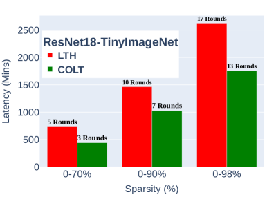
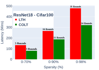
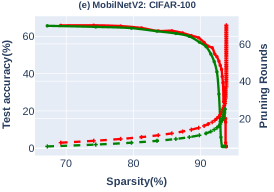
Issues with LTH: Repetitively training from scratch to the convergence of large networks while finding a winning ticket is a costly process, increasing computational time. In Fig. 2, we see that to reach a highly sparse ticket, LTH requires a high no. of pruning rounds (i.e., increasing latency). For example, it takes 62 pruning rounds to generate a 98% sparse ticket of MobileNetV2 on Cifar-100. In this paper, we aim to reduce the number of pruning rounds (training time) to reach such a high sparsity.

3.2 Solution strategy

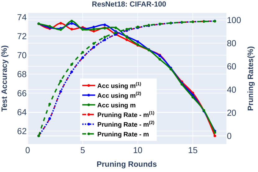
Morcos et al. [22] observed an intriguing fact about LTH regarding the transferability of lottery tickets. Pruned subnetworks, i.e., winning tickets computed using one dataset, can be transferred to other datasets, given the domain of data is similar (e.g., natural images). They argue that the same pruned subnetworks can generalize across different training conditions, optimizers, and datasets. The main implication of this finding is that we can compute a generic winning ticket once using one dataset and then reuse it across multiple datasets or optimizers. It can save the cost of repeatedly computing optimizers or dataset-specific tickets. The winning ticket can achieve similar accuracy and sparsity identical to the winning ticket of the entire model LTH training on the novel dataset. We this paper, we investigate the transferability property of LTH. We observe that intermediate tickets (before obtaining the winning tickets) also have the transferability property but with less sparsity. Each pruning round of our pruning method produces some intermediate subnetworks/tickets, perform the intersection of different subnetworks/tickets, and then transfer the new ticket to the next round. Our concept of transferring tickets across iteration/pruning rounds helps us achieve a similar performance of LTH, costing fewer rounds of computation.

Table 1: Transferring LTH tickets calculated from Partition 1 and 2 to the entire Cifar-100 dataset. The performance of overlapping tickets achieves better sparsity without compromising accuracy. It confirms that overlapping also has transferability property in addition to individual partitions’ tickets.

Using tickets from	Partition-1	Partition-2	Overlapping ticket
Accuracy (%)	72.4	72.3	69.1
Sparsity (%)	79.9	79.9	95.0

Our motivation begins with experiment results shown in Table 1. We divide Cifar-100 into two partitions. Among the 100 classes, images of the first 50 classes remain in one partition and the rest 50 in another. Then we generate LTH tickets (until around 80% sparsity) from each partition. According to [22], both tickets from two separate partitions are transferable to the entire Cifar-100 dataset. Because of this, we achieve 72.4/79.9% and 72.3/79.9% accuracy/sparsity based on training from partitions 1 and 2, respectively. We know there exists a strong correlation between tickets generated by both partitions. It motivates us to check the performance of overlapping tickets, meaning the intersecting sub-network, which remains common after pruning. We notice that even excluding non-overlapping weights (increasing sparsity to 95%), we can still achieve respectable performance (69.1%) on full Cifar-100. It tells that in addition to improving sparsity, overlapping tickets calculated from multiple partitions of the same dataset are also transferrable to the entire dataset. Since intermediate tickets obtained from the intermediate LTH pruning rounds are transferable, we calculate the overlapping ticket of two different partitions in each pruning round. It can provide us with further pruning, which leads us to fewer pruning rounds than LTH, maintaining transferability to individual partitions and the full dataset. In each pruning round, we train two models based on two partitions of the same dataset to calculate two tickets from each partition, then calculate the overlapping tickets between them, and finally, transfer the overlapping ticket to the next pruning round for initialization of those two models. We continue this until the overlapping ticket achieves similar accuracy to the unpruned model.

Figure 3: Transferability of tickets calculated from Partition 1, $m^{(1)}$, partition 2, $m^{(2)}$ and their overlap, $m=m^{(1)}\cap m^{(2)}$. Overlapping ticket, $m$ achieves a higher pruning rate (sparsity), maintaining similar accuracy to others. $m^{(1)}$ and $m^{(2)}$ get matching sparsity because we prune fixed $p\%$ low magnitude weight in every pruning round. In later pruning rounds, the behavior of all tickets is similar because every time the same $m$ calculated from the current round is transferred to both $\mathcal{F}_{1}$ and $\mathcal{F}_{2}$ for the next round making $\theta^{(1)}$ and $\theta^{(2)}$ similar.

tablec

Table 2: A toy example. Initial random weights are updated after training. Using updated weights, we calculate $m^{(1)}$ and $m^{(2)}$ by assigning zero to the locations where (bold values) $p\%$ lower magnitude weights exist. Then, we calculate a generic ticket, $m=m^{(1)}\cap m^{(2)}$, that refers to the pruned subnetwork. Pruned initial weights for the subsequent pruning round are calculated by $m\odot\theta^{(1)}$ and $m\odot\theta^{(2)}$.

Initial weights	After training	Mask	Overlapping mask	Pruned weights
$\theta^{(1)}=$	$\theta^{(1)}=$	$m^{(1)}=$	$m=m^{(1)}\cap m^{(2)}$	$m\odot\theta^{(1)}=$
$\begin{bmatrix}0.1&-0.2&0.9\\ -0.4&0.6&0.8\\ 0.3&0.5&-0.7\end{bmatrix}$	$\begin{bmatrix}0.8&-0.3&0.4 \\ \textbf{-0.1}&\textbf{0.2}&0.7\\ 0.9&0.5&-0.5\end{bmatrix}$	$\begin{bmatrix}1&1&1\\ 0&0&1\\ 1&1&1\end{bmatrix}$	$\begin{bmatrix}1&1&0\\ 0&0&1\\ 1&1&1\end{bmatrix}$	$\begin{bmatrix}0.1&-0.2&0\\ 0&0&0.8\\ 0.3&0.5&-0.7\end{bmatrix}$
$\theta^{(2)}=$	$\theta^{(2)}=$	$m^{(2)}=$		$m\odot\theta^{(2)}=$
$\begin{bmatrix}0.1&-0.2&0.9\\ -0.4&0.6&0.8\\ 0.3&0.5&-0.7\end{bmatrix}$	$\begin{bmatrix}0.9&-0.7&\textbf{0.2}\\ \textbf{-0.1}&0.4&0.5\\ 0.8&0.3&-0.6\end{bmatrix}$	$\begin{bmatrix}1&1&0\\ 0&1&1\\ 1&1&1\end{bmatrix}$		$\begin{bmatrix}0.1&-0.2&0\\ 0&0&0.8\\ 0.3&0.5&-0.7\end{bmatrix}$

3.3 Cyclic Overlapping Lottery Ticket (COLT)

Let $\mathcal{Y}$ be the set of classes in our training dataset $D=\left\{{x}_{i},{y}_{i}\right\}_{i=1}^{n}$, where, $x_{i}\in\mathbb{R}^{h\times w}$ and ${y}_{i}\in\mathcal{Y}$ represent the input image and class label, respectively, and $n$ denotes the number of instances in the dataset. $\mathcal{F}(x;\theta)$ is the unpruned model with all parameters $\theta$. We aim to calculate a winning ticket represented as a sparse mask, $m\in\{0,1\}^{|\theta|}$, such that $\mathcal{F}(x;m\odot\theta)$ can achieve similar accuracy of the unpruned model. We propose a novel approach for generating winning tickets that can be calculated using fewer pruning rounds than LTH. The method has four basic steps below:

(a) Data partitioning: We partition the training data into two non-overlapping halves based on class labels. For this, we randomly split the set of classes $\mathcal{Y}$ into two equal non-overlapping halves $\mathcal{Y}^{(1)}$ and $\mathcal{Y}^{(2)}$, where, $\mathcal{Y}^{(1)}\cap\mathcal{Y}^{(2)}=\emptyset$. Based on the class-specific partition, we create two separate datasets: $D^{(1)}=\left\{{x}^{(1)}_{i},{y}^{(1)}_{i}\right\}_{i=1}^{n^{(1)}}$ and $D^{(2)}=\left\{{x}^{(2)}_{i},{y}^{(2)}_{i}\right\}_{i=1}^{n^{(2)}}$ where, ${y}^{(1)}_{i}\in\mathcal{Y}^{(1)}$ and ${y}^{(2)}_{i}\in\mathcal{Y}^{(2)}$. We prefer the class-based split because it can provide us with more diversity inside intermediate tickets (compared to instance-based alternatives), which will help in faster pruning. Moreover, we split the dataset into only two halves because each half will contain enough instances for generalization. More than two partitions (three/fours) may end up with smaller subsets of the dataset.

(b) Model training: Using the partitioned data $D_{1}$ and $D_{2}$, we train two separate models $\mathcal{F}_{1}(x^{(1)};m\odot\theta^{(1)})$ and $\mathcal{F}_{2}(x^{(2)};m\odot\theta^{(2)})$, respectively. At the first pruning round, $m=1^{|\theta|}$ meaning training of the unpruned model. In later pruning rounds, $m$ will be determined by the mask generation process discussed in the next paragraph, where $m$ will become sparse, containing zeros in the pruned locations. After calculating mask, $m$, we apply the same mask on randomly initialized parameters by $m\odot\theta^{(1)}$ and $m\odot\theta^{(2)}$. The $\odot$ operation is actually performing the pruning because it brings sparsity in weight matrices. At the beginning of the training, parameters $\theta^{(1)}$ and $\theta^{(2)}$ will get exactly the same initial weights as $\theta_{0}\sim\mathcal{D}_{\theta}$ that will later be updated during the course of backpropagation. Therefore, after convergence of models, $\mathcal{F}_{1}$ and $\mathcal{F}_{2}$, both $\theta^{(1)}$ and $\theta^{(2)}$ are expected to contain different weights. A toy example of initial and after training weight of $\theta^{(1)}$ and $\theta^{(2)}$ are shown in Table 2. Note that training of $\mathcal{F}_{1}$ and $\mathcal{F}_{2}$ are independent, meaning a parallel implementation is possible. Moreover, associated datasets $D_{1}$ and $D_{2}$ are smaller than the original ones. It means that we can minimize the overall training time.

(c) Mask generation: Based on the trained weights $\theta^{(1)}$ and $\theta^{(2)}$ from two separate model, we calculate a mask, $m$. First, we generate two intermediate masks, $m^{(1)}$ and $m^{(2)}$ from $\theta^{(1)}$ and $\theta^{(2)}$, respectively. Analyzing the weights of $\theta^{(1)}$, we prune $p\%$ of lower magnitude weights. Thus, the binary mask $m^{(1)}$ will get zeros and ones where weights need to be pruned and not pruned, respectively. Similarly, we generate $m^{(2)}$ from $\theta^{(2)}$. In our experiment, we use $p=20$ as used in LTH [21]. Note we use a small $p$ because a large $p$ gains more sparsity but, at the same time, increases the chance of layer collapse. Now, we generate $m=m^{(1)}\cap m^{(2)}$ to identify overlapping weight locations. $m$ describes the common tickets where both models agree. Our method achieves faster pruning because of the pruning from $p\%$ low-magnitude weights and intersecting masks ($m$) calculated from two different partitions of the dataset. In Fig. 3, we show the performance of $m^{(1)}$, $m^{(2)}$ and $m$ on entire Cifar-100. It shows further evidence that the overlapping ticket, $m$, is transferable across different pruning rounds, ensuring higher sparsity.

(d) Rewinding: In this step, we are transferring the tickets calculated from both partitions to individual partitions of the dataset. Using the calculated $m$ from the previous step, we repeat the process for the subsequent pruning round by iterating to step (b). The same $m$ will modify $\theta^{(1)}$ and $\theta^{(2)}$. Models’ training rewinds the so far unpruned weights (after $\odot$ operation) to their initial values used during the initialization at the beginning of the training. Using the $m$ calculated from the previous round facilitates training such that our method tries to prune within so far unpruned weights only in the next iteration rather than considering all parameters.

Figure 4: Visual illustration of COLT generation. (a) Two models, $\mathcal{F}_{1}$ & $\mathcal{F}_{2}$, of identical architectures, are first initialized with the same initial weights (blue). (b) Next, the two models are trained using the same set of hyperparameters to deduce the final weights (red & green). (c) After training, p% lowest magnitude final weights are pruned from each model. (red weights are the p% lowest magnitude weights while the green ones are above the threshold) (d) Then the models are rewound to their initial state of weights (blue, with the pruned weights being zero. (e) After rewinding, the models’ overlapping weights (blue) are kept, and the rest are pruned. The result is a COLT ticket that can gain accuracies similar to or better than the original network.

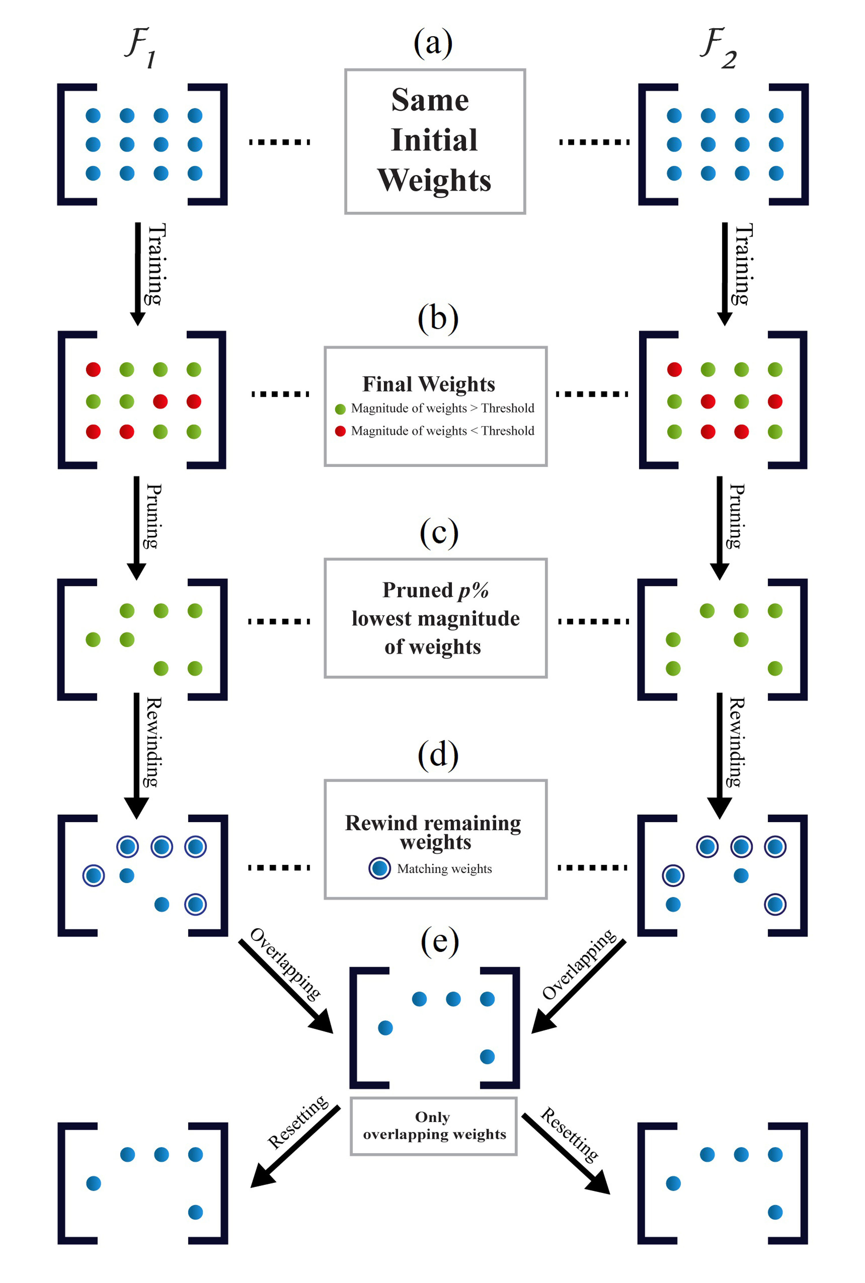
This iterative pruning process will continue until a validation accuracy of the entire dataset, $D$, becomes equal to or better than the accuracy original unpruned model. Because of the train-prune-rewind cycle on the overlapping masks/tickets, we name the ticket generated by our method as Cyclic Overlapping Lottery Ticket (COLT). Fig. 4 provides a visual illustration for generating COLT. Note that we generate COLT based on an architecture that can assign prediction scores for half of the total classes (either $\mathcal{Y}^{(1)}$ or $\mathcal{Y}^{(2)}$ classes). However, we want to evaluate COLT on the entire dataset ($\mathcal{Y}$ classes), which means the same architecture needs to predict scores for all categories. Therefore, to create our final model, $\mathcal{F}$, we removed the winning tickets’ output layer and replaced it with a randomly reinitialized fully connected layer to predict scores for all classes. We then train the tickets until convergence before reporting the final performance on the full dataset.

We outline some key features of our pruning approach. (a) Utilizing transfer property: We investigate the ‘transfer’ property of lottery tickets within different partitions of the same dataset. It helps to confidently identify prospective weights to be pruned in earlier pruning round. (b) Faster pruning: In a single pruning round, our approach performs pruning twice instead of once done by LTH. It enables faster pruning. (c) Avoiding layer collapse: Even after completing pruning two times in a single round, our method can avoid layer collapse [40]. Tickets from the first and second partitions are transferrable and strongly correlate with each other. Thus, intersecting $m^{(1)}$ and $m^{(2)}$ do not discard weights such that a complete layer gets collapsed.

3.4 Pruning heuristics

Pruning heuristics of our proposed method is motivated by previous work [21, 22]. We describe different aspects of our pruning heuristics below:

• Pruning can either be structured or unstructured. Structured pruning discards weights in clusters, i.e., by removing layers/neurons (weight columns), filters, or channels in CNNs. Unstructured pruning does not follow any specific rule, where weights are pruned in a scattered manner to bring sparsity. Since COLTs are generated by selecting the lower magnitude weights from the entire network, they can prune weights from multiple random layers in one pruning round. Therefore, our strategy follows unstructured pruning.

• Based on the strategy used, pruning can be local or global. Local pruning is about pruning a fixed fraction of weights from each layer. In contrast, at each pruning round, global pruning involves pruning a fixed fraction of weights from the entire network allowing each layer to have a different percentage of weights to be discarded. We identify our pruning strategy as global since we treat the whole network at once.

• Pruning can be performed either once (one-shot pruning) or iteratively (iterative pruning). Pruning a significant fraction of the weights in one round can be noisy and eliminate important weights. To overcome this problem, we follow an iterative approach, i.e., several iterations of alternating train-prune cycles with a fraction of the weights pruned at once. This generates significantly better-pruned models and winning tickets [21, 23].

• Our approach uses a novel heuristic to calculate winning tickets from overlapping weights between two models trained on different segments of a dataset. It makes the winning tickets more robust to class variation. Also, it increases the generalizing capability of the tickets while transferring to another dataset.

4 Experiments

4.1 Setup

Datasets: We perform experiments on three image datasets.

(a) Cifar-10 (A & B): Cifar-10 dataset contains 60000 color images (32$\times$32 resolution) belonging to ten classes having 6000 images per class [25]. We have divided it into Cifar-10A (first five classes) and Cifar-10B (remaining five), each consisting of five classes with 5000 and 1000 images per class for training and testing, respectively. Such division is different from previous work done by [22], because they performed experiments by dividing Cifar-10 into parts where each part consisted of all ten classes.

(b) Cifar-100: Cifar-100 [25] dataset is similar to Cifar-10 in terms of image resolution and the total number of images. However, it has 100 classes with 600 images per class. We have configured Cifar-100 similar to the Cifar-10 dataset, where Cifar-100A contains the first 50 classes, and the rest 50 classes are in Cifar-100B. Moreover, each of Cifar-100A and Cifar-100B has 500 images per class for the train set and 100 images per class for the test set.

(c) Tiny ImageNet: Tiny ImageNet dataset [41] is a scaled-down version of ImageNet introduced in the MicroImagenet classification challenge. It has 100000 color images (64$\times$64 resolution) with 200 classes and 500 images per class. Tiny ImageNet has also been divided into two parts called Tiny ImageNet-A and Tiny ImageNet-B. Tiny ImageNet-A contains the first 100 classes, while Tiny ImageNet-B contains the remaining 100 classes.

Table 3: Model architectures examined in this work. Brackets denote residual connections around layers.

Network	Conv-3	MobileNetV2	ResNet-18
Convolution	64,pool 128, pool 256, pool	6$\times$[34,34] 5$\times$[17,17] 8$\times$[9,9] 31$\times$[5,5]	16,3$\times$[16,16] 3$\times$[32,32] 3$\times$[64,64]
FC Layers	100	avg-pool,100	avg-pool,100
All/ Conv weights	397K/371K	2.3M/2.2M	11M
Iteration/Batch	78K / 64	39K / 128	39K / 128
Optimizer	Adam 1.2 e-3	Adam 1.2 e-3	Adam 1.2 e-3
Pruning rate	Conv 15%	Conv 15%	Conv 15%

(a)

(b)

(c)

(d)

(e)

(f)

(g)

(h)

Figure 5: Performance Comparison of LTH and our proposed COLT in terms of accuracy and pruning rounds. Both methods require more pruning rounds to achieve a higher sparsity. However, the accuracy decreases with the increment of sparsity (solid curves). We need a trade-off to balance sparsity and accuracy. For any sparsity level, COLT-based pruning costs fewer pruning rounds in comparison to LTH (dotted curves). Therefore, COLT can prune faster than LTH while maintaining decent accuracy.

Evaluation Process: To evaluate our models, we have used accuracy, Eq. 1 (in percent), which is a standard evaluation metric for image classification. Additionally, to quantitatively determine the sparsity of our models, we have used prune rate, Eq. 2 (in percent) that gives the percentage of parameters that are zero out of all the parameters of a model. Our iterative pruning algorithm runs until a desired $PruneRate$ is reached. Each iteration of the pruning algorithm runs for fifty epochs, and the best model (with the lowest validation loss) is selected.

$$Accuracy=\mathit{\frac{Number\>of\>correct\>predictions}{Total\>number\>of\>predictions}\times 100}$$ (1)

$$PruneRate=\mathit{\frac{Number\>of\>zero\>params}{Total\>number\>of\>params}\times 100}$$ (2)

Model Architecture: We have used three models for conducting experiments: Conv-3, ResNet-18, and MobileNetV2 (see Table 3). We have used the Conv and ResNet architectures since they were tested in LTH [21]. We have used the MobileNet architecture because it is a lightweight deep-learning model with few parameters and high classification performance. Conv-3 model architecture is a scaled-down version of VGG [42] consisting of about 0.37M parameters. It has three convolutional layers, followed by one linear output layer. Besides, we include a batch normalization layer followed by max-pooling after each convolution layer. The ResNet-18 architecture consists of 72 layers with 18 deep residual connection layers [23] and about 11.1M parameters. MobileNetV2 [24] architecture consists of 53 layers with 19 residual bottleneck layers and about 2.2M parameters. We use Xavier or Glorot weight initialization technique for all the models [43]. For all three models, the last layer is a fully-connected output layer from the global average pool of the final convolution layer to the number of output classes as done in [21, 23]. The last convolutional layer was globally average pooled to ensure that we could transfer the weights of a model trained on one dataset to another dataset of a different input shape without bringing any modifications to the model. We trained all three models on Cifar-10 and Cifar-100, whereas Conv-3 is excluded from Tiny ImageNet because it is too shallow to train on Tiny ImageNet.

Implementation details: After training and pruning, weights need to be reset to their initial values at the beginning of training (training iteration 0) to generate winning tickets [21]. However, Frankle et al. [21] have found that this only works for shallow models. For deeper models, a learning rate warmup is necessary, along with weight resetting to generate winning tickets. So, our experiments used a learning rate warmup for the first epoch. We globally pruned only the convolutional layers at a rate of 0.2 (20%) for LTH and 0.15 (15%) for COLT per iteration. Similarly, we did not prune the linear output layers as it comprises only a tiny fraction of the whole network. Each model was trained for 50 epochs with a batch size of 256 and a learning rate of 0.1. The learning rate was annealed by a factor of 5 at 20, 30, and 45 epochs. Conv-3 models were trained using Stochastic Gradient Descent (SGD) with a momentum of 0.9 and weight decay of 0.0005. All other models were trained using an Adam optimizer with betas of 0.9 and 0.999 and weight decay of 0.0001. We implement this work with PyTorch framework.

4.2 Compared methods

We compare our work with the three methods discussed as follows: (1) Unpruned network: The unpruned network is the original CNN (Conv-3/Mobilenetv2/Resnet-18) trained until convergence, where no pruning strategy is considered during the learning process. We initialize their weights using the Xavier/Glorot weight initialization technique [43]. We assume that an unpruned network is generally overparameterized and, therefore, a pruning method is needed to discard unnecessary weights. (2) Lottery Ticket Hypothesis (LTH) [21]: To compare with LTH, we also generated LTH tickets. We pruned 20% weights after each training iteration and then rewound them to their initial state. We then compare their performance with COLT tickets in Sec. 4.3. [21] and [22] have shown that random tickets with and without masking preserved results in lower performance than winning tickets with equal parameters. As a result, we have omitted using random tickets while evaluating COLT tickets and directly compared COLT tickets with LTH tickets.(3) Morcos et al. [22]: Winning tickets are computationally expensive to generate because of the repetitive train-prune-rewind cycle. Morcos et al. have shown that once generated from a dataset, winning tickets can be transferred to another dataset, bypassing the need to find separate winning tickets for each dataset. Concretely, they observed that transferring the winning tickets from one dataset to another can achieve almost similar performance to the winning tickets generated on the same dataset. They have shown that winning tickets generalize well in the natural image domain. Moreover, they have also demonstrated winning tickets generated from large datasets consistently transferred better than those generated using small datasets.

(a)

(b)

(c)

(d)

(e)

(f)

Figure 6: Performance comparison of COLT with Morocos et al. [22] when transferring tickets calculated from one dataset to another. Both methods’ performance declines slightly when the tickets reach high sparsities. However, when tickets are transferred from a large dataset (TinyImageNet) to small datasets (Cifar-10, Cifar-100), COLT (green curve) consistently outperforms Morcos et al. (red curve) at high sparsities.

4.3 Main Results

We generate COLT and LTH tickets for ResNet-18 and MobileNetV2 on Cifar-10, Cifar-100, and Tiny ImageNet. For Conv-3, we obtain tickets for Cifar-10 and Cifar-100 only following [21]. For the weight transferability experiment, we transfer the tickets calculated from Tiny ImageNet to Cifar-10 and Cifar-100. Again, we transfer the tickets from Cifar-100 to Cifar-10. All the experiments generating COLT and LTH tickets are repeated multiple times with a different random initialization, and we reported the best scores.

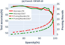
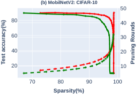
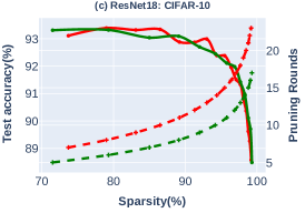
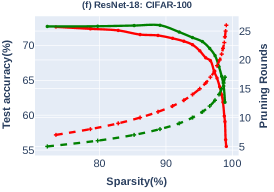
Results on Cifar-10: We observe that the accuracy of COLT and LTH are level pegging for ResNet-18. For Conv-3 tickets (Fig. 5(a)), we notice a similar picture with both COLT and LTH performing equally. For MobileNetV2 (Fig. 5(b)), we see that the performance of COLT and LTH are similar till the pruning rate of 70%, and then the performance of COLT tickets starts decreasing compared to LTH tickets. For both methods, the performance of the tickets drops steeply when the pruning rate is higher than 95% for Conv-3, 90% for MobileNetV2, and 96% for ResNet-18. For all tickets, COLT consistently requires fewer pruning rounds than LTH to generate a particular sparse ticket. For example, to reach 70% sparsity, COLT needs 3, 1, and 2 fewer rounds than LTH on Conv-3, MobileNetV2, and ResNet-18, respectively. Similarly, to achieve 90% sparsity, COLT requires 4, 2, and 3 fewer rounds than LTH on Conv-3, MobileNetV2, and ResNet-18, respectively. Lastly, to reach 98% sparsity, COLT needs 9, 2, and 5 fewer rounds than LTH on Conv-3, MobileNetV2, and ResNet-18, respectively. Because of the pruning of non-overlapping weights in COLT, it consistently requires fewer rounds than LTH to generate sparse winning tickets. COLT also retains a similar performance to LTH as these non-overlapping weights are unimportant, and excluding those weights does not affect the overall performance much.

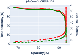
Results on Cifar-100: Observing Fig.. 5(f), the performance of COLT and LTH tickets is similar until a prune rate of 80% for ResNet-18. However, after 80% pruning, the COLT-based tickets perform better than LTH tickets. For MobileNetV2 (Fig.. 5(e)) and Conv-3 Fig.. 5(d), the performance of COLT and LTH tickets are almost similar, with LTH slightly outperforming COLT at some prune rates. In addition, the accuracy of the LTH and COLT tickets starts to drop drastically when the pruning rate is greater than 95% for Resnet-18, 85% for MobileNetV2, and 90% for Conv-3. Besides, COLT regularly generates winning tickets in fewer pruning rounds than LTH. To reach 70% sparsity, COLT requires 3, 2, and 2 fewer rounds than LTH on Conv-3, MobileNetV2, and ResNet-18, respectively. To achieve 90% sparsity, COLT requires 6, 6, and 3 fewer rounds than LTH on Conv-3, MobileNetV2, and ResNet-18, respectively. Lastly, to reach 98% sparsity, COLT needs 9, 8, and 6 fewer rounds than LTH on Conv-3, MobileNetV2, and ResNet-18, respectively. This becomes possible due to COLT’s aggressive non-matching weights pruning strategy at each round. Moreover, COLT preserves accuracy as the non-matching weights are insignificant and do not hamper the accuracy.

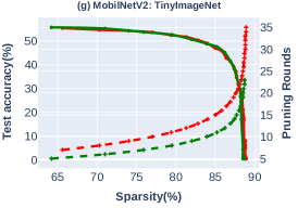
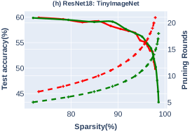
Results on Tiny ImageNet: Analyzing Fig. 5(g) and 5(h), we can observe that the performance of COLT and LTH tickets are similar for most of the tickets, with COLT tickets slightly performing better than LTH Tickets at some sparsities. Apart from that, both tickets’ accuracy drops significantly from 85% for ResNet-18 and from 75% for MobileNetV2. Looking at the pruning rounds, we can see that COLT always generates sparse tickets at fewer iterations than LTH. To reach 70% sparsity, COLT requires two fewer rounds than LTH on MobileNetV2 and ResNet-18. To reach 90% sparsity, COLT requires 9 and 3 fewer rounds than LTH on MobileNetV2 and ResNet-18, respectively. Finally, to reach 98% sparsity, COLT requires 4 and 6 fewer rounds than LTH on MobileNetV2 and ResNet-18, respectively. As COLT prunes a higher rate of redundant weights than LTH at each iteration, it can generate winning tickets in fewer rounds than LTH without compromising accuracy.

4.4 Transferring LTH & COLT Tickets Across Datasets

The iterative process of ticket generation can be costly. To mitigate this problem, Morcos et al. [22] showed that winning tickets (pruned subnetwork) generated on larger, more complex datasets could generalize substantially better than those generated on small datasets. In other words, we do not need to create tickets for each dataset. Tickets generated from one larger dataset can be transferred/employed again to train the same network for a smaller dataset. For this reason, we perform experiments to transfer the COLT and LTH tickets of Tiny ImageNet to Cifar-10 and Cifar-100. Since we are using datasets with different input shapes, there will be a weight mismatch when transferring weights of the linear layer. To overcome this problem, we have globally average pooled the output from the last convolutional layer before passing it through the dense output layer. [22] further showed that just increasing the number of classes while keeping the dataset size fixed can significantly improve the generalization capability of winning tickets. To verify this point, in our work, we have transferred the COLT and LTH tickets of Cifar-100 to Cifar-10, since they are with the same size, but Cifar-100 has more classes than Cifar-10.

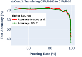
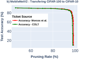
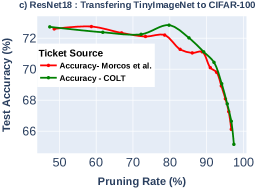
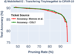
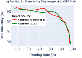
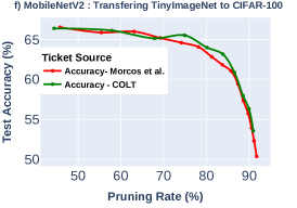
Observing Fig. 6, we can see that as COLT and Morcos et al. reach high sparsities, the accuracy slowly deteriorates. However, COLT consistently performs better than Morcos et al. at high sparsities when TinyImageNet tickets are transferred to Cifar-10 & Cifar-100. Additionally, both methods are on par and work well when Cifar-100 tickets are transferred to Cifar-10 for all sparsities. Therefore, we claim that COLT tickets have a high generalization capacity and transferability to other datasets of a similar domain.

One can compare the performance of regular tickets (COLT) with transferred tickets by analyzing Fig. 5 and 6. We observe that the performance trend for regular and transferred tickets is similar across architectures and datasets. If a regular ticket performs well on a dataset, the transferred ticket also performs well, and vice versa. The bottom line is that we can generate COLT tickets from one dataset and then use the same ticket to train another dataset of a similar domain without compromising network performance.

Table 4: State-of-the-art results describing the performance comparison of tickets generated by the original unpruned network, LTH, and COLT. The tickets were generated and evaluated on TinyImageNet and then transferred to Cifar-10 and Cifar-100. We compare sparse tickets from three methods on ResNet-18 and MobileNetV2 architectures. $\uparrow$ ($\downarrow$) means higher (lower) is better. “-” denotes results that are not applicable there.

Model: ResNet18 and Dataset: Tiny ImageNet
Method	Acc. $\uparrow$	Pruning $\uparrow$	Latency $\downarrow$	No of Pruning $\downarrow$
	(%)	Rate (%)	(minutes)	Rounds
Unpruned	59.9	0	-	-
LTH	53.2	97.3	2625	18
Ours (COLT)	53.9	97.2	1756	12
Tickets transformed from TinyImageNet to Cifar10
Unpruned	93.4	0	-	-
Morcos et al. [22]	89.9	97.1	-	-
Ours (COLT)	90.5	97.1	-	-
Tickets transformed from TinyImageNet to Cifar100
Unpruned	73.2	0	-	-
Morcos et al. [22]	64.8	97.3	-	-
Ours (COLT)	65.2	97.4	-	-

Model: MobileNetV2 and Dataset: Tiny ImageNet
Acc. $\uparrow$	Pruning $\uparrow$	Latency $\downarrow$	# of Pruning $\downarrow$
(%)	Rate (%)	(minutes)	Rounds
56.1	0	-	-
54.7	70.3	856	7
55.2	71.0	354	5
Tickets transformed from TinyImageNet to Cifar10
90.6	0	-	-
88.9	78.0	-	-
89.2	78.8	-	-
Tickets transformed from TinyImageNet to Cifar100
65.8	0	-	-
64.1	74.1	-	-
65.5	74.9	-	-

4.5 State-of-the-art comparison

Table 4 compares the results of unpruned network, COLT, and LTH methods in terms of no. of pruning rounds, accuracy, and latency. For the transferability experiment, tickets were generated using TinyImageNet and transferred to Cifar10 and Cifar100. In line with [22], we notice transferring tickets from a large (TinyImageNet) to a small dataset (Cifar10 ) results in better performance than vice versa. We report results on ResNet-18 and MobileNetV2 architectures. For ResNet18, we still get good accuracy, even after pruning 97.2% parameters. It indicates that even with just 2.8% of the weights left in ResNet18, we continue to achieve a decent level of accuracy. It implies that a model does not require all the parameters to get the desired accuracy. As shown in Table 4, COLT can achieve better accuracy than LTH maintaining high sparsity. Moreover, COLT needs fewer pruning rounds and noticeably less time than LTH. However, we differ from the unpruned network accuracy by 5–6%. The reason is that after 97% pruning, some important weights may have been pruned, resulting in a decrease in accuracy. There is a high risk of layer collapse for unstructured pruning when weights are pruned at high sparsity. According to Tanaka et al.[40], iterative magnitude pruning prevents such layer collapse by promoting the magnitude scores generated from gradient descent to follow a conservation law, which, when combined with iteration, causes the relative scores for the largest layers to rise during pruning. In this regard, COLT performs comparatively better than LTH, even if it receives fewer iterations to prune at high sparsity. Therefore, we claim that COLT can retain “good weights” even after pruning at high sparsities. On the other hand, MobileNet has nine million fewer weights than ResNet18. As a result, unlike an unpruned network, neither LTH nor COLT achieves par accuracy at high sparsity.

However, we can get about the same accuracy with a prune rate of 71% as compared to an unpruned network. Likewise, in ResNet18, we generate tickets much faster and with fewer pruning rounds than the LTH. In this case, LTH takes eight pruning rounds and 856 minutes to generate a 70.3% sparse ticket that obtains an accuracy of 54.7% on the TinyImageNet dataset. In contrast, COLT only needed five pruning rounds and 354 minutes to generate a ticket that was 71% sparse and had an accuracy of 55.2%. For MobileNetV2 and ResNet18, COLT takes significantly less time than LTH. There are fewer pruning rounds, and computing gradients take less time. COLT generates sparser tickets than LTH in every iteration. Hence we need to compute fewer gradients than LTH. As a result, we can generate a ticket with COLT much faster than we can with the LTH.

A similar trend is observed when the tickets are transferred to Cifar-10 and Cifar-100. For medium sparsity tickets (prune rate around 80%). Particularly for MobileNetV2, both COLT and Morcos et al. [22] have accuracies close to the original unpruned network. It implies that we can adopt a network that has already been pruned on one dataset and transfer it to another dataset with an accuracy comparable to an unpruned network. Moreover, we do not need additional resources to prune the network for each individual dataset. In contrast, for high-sparsity tickets, the accuracy decreases by about 3% when transferred to Cifar-10 and by about 8% when transferred to Cifar-100. However, COLT appears to become more generic than Morcos et al. [22]. This is because COLT retains the overlapping weights of two networks trained on two one-half splits of a dataset, making the COLT tickets more robust to image variations.

Figure 7: The similarity (blue bars) of pruned weights between sparse tickets calculated by COLT and LTH method. With the increase of sparsity, both kinds of methods prune similar weights. To achieve this, COLT requires fewer training rounds than LTH (red vs. green curve).

4.6 Discussion

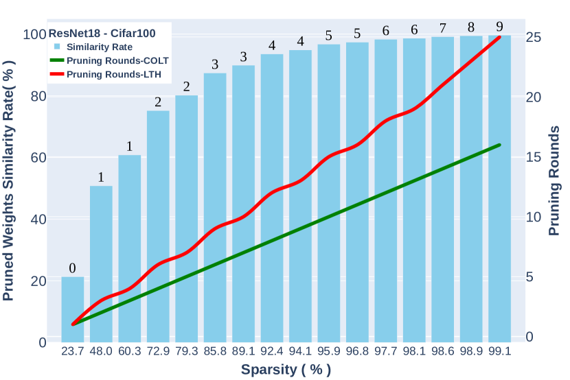
Weight Similarity Analysis: Fig. 7 depicts a comparison between LTH and COLT in terms of pruned weights similarity and pruning rounds for the ResNet-18 model on the Cifar-100 dataset. The X-axis represents the sparsities in percentage. The Y-axis on the left represents the pruning rate similarity of unpruned weights, and the Y-axis on the right represents the pruning rounds taken to generate a ticket of the same sparsity. The blue bars represent the similarity in the pruned weights between LTH and COLT tickets. The similarity is calculated at the beginning of each pruning round. COLT and LTH tickets are initialized with the same weights. The similarity rate is the number of common pruned parameters between COLT and LTH divided by the total no. of initial parameters. Here ‘common’ implies that LTH and COLT pruned the same weights. The red and green line joining the bars represents the pruning rounds required by COLT and LTH, respectively. The numbers on the top of the bars depict the additional pruning rounds required by LTH compared to COLT. We find substantially fewer identical remaining weights between COLT and LTH during the early stages. However, as the prune rate increases, the similarity between the remaining weights of LTH and COLT also increases. For example, at the 28% pruning rate, the similarity of remaining weights is 20%. Subsequently, the similarity of remaining weights jumps to 50% when the sparsity of tickets reaches around 48%. It implies that identical weights between COLT and LTH start getting pruned while the weight matrix becomes sparse. In other words, LTH and COLT essentially prune similar weights to generate a sparse winning ticket. However, COLT (solid red line) requires fewer pruning rounds than LTH (solid green line) to create a ticket of the same sparsity. For example, to reach a sparsity of about 89%, LTH requires three more pruning rounds than COLT, making the LTH process time-consuming.

Performance Analysis: Analyzing all the results, we can see that COLT tickets generated from large models like ResNet-18 perform on par or even at times better than LTH tickets, regardless of the dataset size. Even when these COLT tickets are transferred to other datasets, they still can generalize well and give accuracies close to the original network at high sparsities. Observing the performance of COLT tickets of MobileNetV2, those tickets slightly underperform on small datasets like Cifar-10 and Cifar-100 compared to LTH tickets. However, the accuracy of COLT tickets of MobileNetV2 is similar to the LTH tickets when generated on large datasets like Tiny ImageNet. Moreover, when these Tiny ImageNet tickets of MobileNetV2 are transferred to small datasets like Cifar-10 and Cifar-100, their performance is similar to or at times better than LTH tickets. Conv-3 is a very shallow model compared to MobileNetV2 and ResNet-18. Analyzing COLT tickets of Conv-3, we can observe that they perform on a similar level to LTH tickets, not only on the respective datasets but also while transferring Cifar-100 tickets to Cifar-10.

5 Conclusion

In this paper, we proposed a new set of lottery tickets termed COLT to prune deep neural networks. Like tickets from LTH, COLTs can achieve high sparsity and weights’ transferability across datasets without compromising accuracy. We compute COLTs by leveraging tickets obtained from two class-wise partitions of a dataset. We notice that the performance of these tickets is on par with the LTH-generated lottery tickets in terms of accuracy. Moreover, COLTs are generated at fewer iterations than LTH tickets. In experiments, we have also demonstrated that COLTs generated on a large dataset (Tiny ImageNet) can be transferred to a small dataset (Cifar-10, Cifar-100) without compromising performance, showing these tickets’ generalizing capability. Future works in this line of investigation may consider COLT’s sparsity and transferability on deeper architectures (VGG16/DenseNet/ShuffleNet) and vast datasets (ImageNet/MSCOCO). Moreover, one can explore different problem setups like object detection and segmentation in the context of network pruning.

References

- [1] M. C. Mozer and P. Smolensky, “Using Relevance to Reduce Network Size Automatically,” Connection Science, vol. 1, pp. 3–16, 1989.
- [2] E. Karnin, “A Simple Procedure for Pruning Back-propagation Trained Neural Networks,” IEEE Transactions on Neural Networks, vol. 1, no. 2, pp. 239–242, 1990.
- [3] S. Han, J. Pool, J. Tran, and W. J. Dally, “Learning both weights and connections for efficient neural networks,” in Proceedings of the 28th International Conference on Neural Information Processing Systems - Volume 1, ser. NIPS’15. Cambridge, MA, USA: MIT Press, 2015, p. 1135–1143.
- [4] H. Li, A. Kadav, I. Durdanovic, H. Samet, and H. P. Graf, “Pruning filters for efficient convnets,” in International Conference on Learning Representations, 2017.
- [5] Y. LeCun, J. Denker, and S. Solla, “Optimal brain damage,” in Advances in Neural Information Processing Systems, D. Touretzky, Ed., vol. 2. Morgan-Kaufmann, 1989, pp. 598–605.
- [6] B. Hassibi and D. G.Stork, “Second Order Derivatives for Network Pruning: Optimal Brain Surgeon,” Adv Neural Inform Proc Syst, vol. 5, 10 1992.
- [7] G. Hinton, O. Vinyals, J. Dean et al., “Distilling the knowledge in a neural network,” arXiv preprint arXiv:1503.02531, vol. 2, no. 7, 2015.
- [8] P. Molchanov, S. Tyree, T. Karras, T. Aila, and J. Kautz, “Pruning convolutional neural networks for resource efficient inference,” in 5th International Conference on Learning Representations, ICLR 2017, Toulon, France, April 24-26, 2017, Conference Track Proceedings. OpenReview.net, 2017.
- [9] T.-J. Yang, Y. hsin Chen, and V. Sze, “Designing energy-efficient convolutional neural networks using energy-aware pruning,” 2017 IEEE Conference on Computer Vision and Pattern Recognition (CVPR), pp. 6071–6079, 2017.
- [10] J.-H. Luo, J. Wu, and W. Lin, “Thinet: A filter level pruning method for deep neural network compression,” in 2017 IEEE International Conference on Computer Vision (ICCV), 2017, pp. 5068–5076.
- [11] B. O. Ayinde, T. Inanc, and J. M. Zurada, “Redundant feature pruning for accelerated inference in deep neural networks,” Neural Netw., vol. 118, no. C, p. 148–158, oct 2019.
- [12] Y. Guo, A. Yao, and Y. Chen, “Dynamic network surgery for efficient dnns,” Advances in neural information processing systems, vol. 29, 2016.
- [13] D. Molchanov, A. Ashukha, and D. P. Vetrov, “Variational dropout sparsifies deep neural networks,” in ICML, 2017.
- [14] Z. Qin, F. Yu, C. Liu, L. Zhao, and X. Chen, “Interpretable Convolutional Filter Pruning,” ArXiv, vol. abs/1810.07322, 2018.
- [15] M. Zhu and S. Gupta, “To prune, or not to prune: Exploring the efficacy of pruning for model compression,” in 6th International Conference on Learning Representations, ICLR 2018, Vancouver, BC, Canada, April 30 - May 3, 2018, Workshop Track Proceedings. OpenReview.net, 2018.
- [16] M. Mondal, B. Das, S. D. Roy, P. Singh, B. Lall, and S. D. Joshi, “Adaptive cnn filter pruning using global importance metric,” Computer Vision and Image Understanding, vol. 222, p. 103511, 2022.
- [17] Q. Tian, T. Arbel, and J. J. Clark, “Structured deep fisher pruning for efficient facial trait classification,” Image and Vision Computing, vol. 77, pp. 45–59, 2018.
- [18] X. Lin, S. Kim, and J. Joo, “Fairgrape: Fairness-aware gradient pruning method for face attribute classification,” in European Conference on Computer Vision. Springer, 2022, pp. 414–432.
- [19] F. Jia, X. Wang, J. Guan, H. Li, C. Qiu, and S. Qi, “Arank: Toward specific model pruning via advantage rank for multiple salient objects detection,” Image and Vision Computing, vol. 111, p. 104192, 2021.
- [20] M. Bonnaerens, M. Freiberger, and J. Dambre, “Anchor pruning for object detection,” Computer Vision and Image Understanding, p. 103445, 2022.
- [21] J. Frankle and M. Carbin, “The lottery ticket hypothesis: Finding sparse, trainable neural networks,” in 7th International Conference on Learning Representations, ICLR 2019, New Orleans, LA, USA, May 6-9, 2019. OpenReview.net, 2019.
- [22] A. S. Morcos, H. Yu, M. Paganini, and Y. Tian, One Ticket to Win Them All: Generalizing Lottery Ticket Initializations across Datasets and Optimizers. Red Hook, NY, USA: Curran Associates Inc., 2019.
- [23] K. He, X. Zhang, S. Ren, and J. Sun, “Deep residual learning for image recognition,” 2016 IEEE Conference on Computer Vision and Pattern Recognition (CVPR), pp. 770–778, 2016.
- [24] M. Sandler, A. Howard, M. Zhu, A. Zhmoginov, and L.-C. Chen, “Mobilenetv2: Inverted residuals and linear bottlenecks,” in 2018 IEEE/CVF Conference on Computer Vision and Pattern Recognition, 2018, pp. 4510–4520.
- [25] A. Krizhevsky and G. Hinton, “Learning Multiple Layers of Features from Tiny Images,” University of Toronto, Toronto, Ontario, Tech. Rep. 0, 2009.
- [26] T. Gale, E. Elsen, and S. Hooker, “The state of sparsity in deep neural networks,” ArXiv, vol. abs/1902.09574, 2019.
- [27] N. Lee, T. Ajanthan, and P. Torr, “SNIP: SINGLE-SHOT NETWORK PRUNING BASED ON CONNECTION SENSITIVITY,” in International Conference on Learning Representations, 2019.
- [28] Z. Allen-Zhu, Y. Li, and Y. Liang, Learning and Generalization in Overparameterized Neural Networks, Going beyond Two Layers. Red Hook, NY, USA: Curran Associates Inc., 2019.
- [29] Z. Allen-Zhu, Y. Li, and Z. Song, “A convergence theory for deep learning via over-parameterization,” in Proceedings of the 36th International Conference on Machine Learning, ser. Proceedings of Machine Learning Research, K. Chaudhuri and R. Salakhutdinov, Eds., vol. 97. PMLR, 09–15 Jun 2019, pp. 242–252.
- [30] S. Du and J. Lee, “On the power of over-parametrization in neural networks with quadratic activation,” in Proceedings of the 35th International Conference on Machine Learning, ser. Proceedings of Machine Learning Research, J. Dy and A. Krause, Eds., vol. 80. PMLR, 10–15 Jul 2018, pp. 1329–1338.
- [31] S. S. Du, X. Zhai, B. Póczos, and A. Singh, “Gradient descent provably optimizes over-parameterized neural networks,” in 7th International Conference on Learning Representations, ICLR 2019, New Orleans, LA, USA, May 6-9, 2019. OpenReview.net, 2019.
- [32] B. Neyshabur, R. Tomioka, and N. Srebro, “In search of the real inductive bias: On the role of implicit regularization in deep learning.” in ICLR (Workshop), 2015.
- [33] B. Neyshabur, Z. Li, S. Bhojanapalli, Y. LeCun, and N. Srebro, “The role of over-parametrization in generalization of neural networks,” in International Conference on Learning Representations, 2019.
- [34] R. Van Soelen and J. W. Sheppard, “Using Winning Lottery Tickets in Transfer Learning for Convolutional Neural Networks,” in 2019 International Joint Conference on Neural Networks (IJCNN). IEEE, 2019, pp. 1–8.
- [35] S. Kornblith, J. Shlens, and Q. V. Le, “Do better imagenet models transfer better?” in 2019 IEEE/CVF Conference on Computer Vision and Pattern Recognition (CVPR). Los Alamitos, CA, USA: IEEE Computer Society, jun 2019, pp. 2656–2666.
- [36] C. Tan, F. Sun, T. Kong, W. Zhang, C. Yang, and C. Liu, “A survey on deep transfer learning,” in Artificial Neural Networks and Machine Learning – ICANN 2018, V. Kůrková, Y. Manolopoulos, B. Hammer, L. Iliadis, and I. Maglogiannis, Eds. Cham: Springer International Publishing, 2018, pp. 270–279.
- [37] J. Yosinski, J. Clune, Y. Bengio, and H. Lipson, “How transferable are features in deep neural networks?” in Advances in Neural Information Processing Systems, Z. Ghahramani, M. Welling, C. Cortes, N. Lawrence, and K. Weinberger, Eds., vol. 27. Curran Associates, Inc., 2014.
- [38] B. Zoph, V. Vasudevan, J. Shlens, and Q. V. Le, “Learning transferable architectures for scalable image recognition,” 2018 IEEE/CVF Conference on Computer Vision and Pattern Recognition, pp. 8697–8710, 2018.
- [39] H. Zhou, J. Lan, R. Liu, and J. Yosinski, “Deconstructing lottery tickets: Zeros, signs, and the supermask,” Advances in neural information processing systems, vol. 32, 2019.
- [40] H. Tanaka, D. Kunin, D. L. K. Yamins, and S. Ganguli, “Pruning neural networks without any data by iteratively conserving synaptic flow,” in Proceedings of the 34th International Conference on Neural Information Processing Systems, ser. NIPS’20. Red Hook, NY, USA: Curran Associates Inc., 2020.
- [41] Y. Le and X. S. Yang, “Tiny ImageNet Visual Recognition Challenge,” 2015.
- [42] K. Simonyan and A. Zisserman, “Very deep convolutional networks for large-scale image recognition,” CoRR, vol. abs/1409.1556, 2015.
- [43] X. Glorot and Y. Bengio, “Understanding the difficulty of training deep feedforward neural networks,” in AISTATS, 2010.