Hypertracking and Hyperrejection: Control of Signals beyond the Nyquist Frequency

Abstract

This paper studies the problem of signal tracking and disturbance rejection for sampled-data control systems, where the pertinent signals can reside beyond the so-called Nyquist frequency. In light of the sampling theorem, it is generally understood that manipulating signals beyond the Nyquist frequency is either impossible or at least very difficult. On the other hand, such control objectives often arise in practice, and control of such signals is much desired. This paper examines the basic underlying assumptions in the sampling theorem and pertinent sampled-data control schemes, and shows that the limitation above can be removed by assuming a suitable analog signal generator model. Detailed analysis of multirate closed-loop systems, zeros and poles are given, which gives rise to tracking or rejection conditions. Robustness of the new scheme is fully characterized; it is shown that there is a close relationship between tracking/rejection frequencies and the delay length introduced for allowing better performance. Examples are discussed to illustrate the effectiveness of the proposed method here.

I Introduction

It is well recognized that sampled-data control systems are inherently limited in resolution in time, due to sampling. This is clearly seen from the classical sampling theorem, e.g., [16]; there Shannon showed that the original analog signal can be perfectly reconstructed if the signal is perfectly band limited below the so-called Nyquist frequency, i.e., half the sampling frequency.

In spite of such well-established developments, there are many practical needs to process signals that go beyond the Nyquist frequency. Superresolution in image processing is one such example. In control as well, we are often confronted with such requirements. For example,

• tracking a high-frequency sinusoid in regulating AC power current to a prespecified frequency (particularly in micro-grid systems),

• rejection of high-frequency disturbance generated by disk rotation in hard-disk drives [3, 30], or

• laser sintering manufacturing systems [9, 20], vision-guided high-speed controls [17], etc.

Due to the limited resolution in time, such objectives have been regarded as either impossible or at least ill posed [27]. However, if we examine the sampling theorem, it is clear that the band-limitation below the Nyquist frequency is only a sufficient condition for perfect signal reconstruction. A different type of band-limiting hypothesis can lead to a different signal reconstruction result; see, e.g., [22]. Indeed, by using modern sampled-data control theory, we have developed a new paradigm for digital signal processing, including superresolution [28].

The present work is motivated by the above observation, and intends to give a solution to the control problems as listed above. More specifically, we study high-frequency tracking and disturbance rejection of signals beyond the Nyquist frequency. The basic philosophy remains the same as that of [28], with the differences that the tracking or rejection signals must be precise, and we must also form a closed-loop system. Robustness becomes a crucial issue here.

In view of the new feature of tracking or rejecting signals beyond the Nyquist frequency, we call the present control scheme hypertracking or hyperrejection to highlight the difference with conventional tracking/rejection problems in sampled-data control.

The basic concept of the present study for hypertracking was first presented in [29]. This paper is a continuation with a complete characterization of robustness, which gives a new insight (see Section V) to us. A related study concerning multiple signals was also given in [21] in a different setting. We also note that the recent article [20] has proposed a multirate control scheme to reject the disturbance beyond the Nyquist frequency in a mechatronic system. However, the optimized intersample behavior and the robustness are not addressed there.

Notation

In denoting function values, we will adopt the following convention: for a function $f$ with a continuous-time variable $t$, we write $f(t),$ while we write $g[k]$ with square brackets when $k$ takes on integer values.

II Problem Formulation

Consider the sampled-data system depicted in Fig. 1.

Figure 1: Sampled-data feedback system with input disturbance

$P(s)$ is a linear, time-invariant, strictly proper, continuous-time plant, and $K(z)$ is a linear, time-invariant, discrete-time controller. The error $e$ is sampled with sampling period $h$, and after sampled, it is upsampled by factor $M$ to allow for a faster control processing. The role of the action (upsampler) of $\uparrow M$ is to increase the sampling rate by the factor $M$ by placing $M-1$ equally spaced zeros between each pair of samples as follows ([8, 18]):

$$(\mbox{$\mbox{$\uparrow M$}$})(e)[k]=\begin{cases}e[k/M]&\mbox{ if $k=mM$ for some integer $m$}\\ 0&\mbox{ otherwise}.\end{cases}$$

Note that in the present case, the sampled sequence $\{e[k]\}_{k=1}^{\infty}$ synchronizes with continuous-time signals every $h$ seconds, hence $e[k]$ enters into the system as $e(kh)$ for every $k$. With this convention, the action of the above upsampler takes the following form:

$$(\mbox{$\mbox{$\uparrow M$}$})(e)(kh+\ell)=\begin{cases}e(kh)&\text{if }\ell=0\\ 0&\text{if }\ell=\nicefrac{{h}}{{M}},\ldots,\nicefrac{{(M-1)h}}{{M}}.\end{cases}$$ (1)

${\cal H}_{h/M}$ is the zero-order hold that holds the output as constant for the period of $h/M$.

We now consider the following problem:

Problem 1: In the block diagram Fig. 1, consider the reference input $\sin\omega_{r}t$ and the disturbance input $\sin\omega_{d}t$ where $\omega_{r}$ and $\omega_{d}$ are either below or above the Nyquist frequency $\pi/h$. Find a discrete-time controller $K(z)$ such that the output $y$ that tracks the reference $r(t)=\sin\omega_{r}t$ or its delayed signal $r(t-L)$ for some $L>0$, and also rejects the disturbance $d(t)$. Here the tracking may be only approximate due to the sample-hold nature in Fig. 1. However, the error due to this approximation becomes small for a large $M$ or small $h$ ([26]).

When $\omega_{r}$ or $\omega_{d}$ is above the Nyquist frequency, this problem does not fall into the conventional sampled-data control paradigm. Such signals appear in measurement as aliased components below the Nyquist frequency, and are mixed with other system signals already existent in the base-band (i.e., lower than the Nyquist frequency) range. The prime objective of the present paper is to provide a scheme that enables us to achieve the above goal.

III Hypertracking and Tracking Conditions

We now proceed to give a solution to the hypertracking problem. We first give a state-space description of Fig. 1, assuming $d\equiv 0$, characterize its zeros for tracking, and then proceed to a design method and examples in the subsequent sections.

III-A State-space description of the lifted multirate system

We first describe the system in Fig. 1 as a time-invariant discrete-time system with a single sampling period $h$.

Let $P(s)$ and $K(z)$ be described by the following state-space equations:

$$P(s):\left\{\begin{array}[]{@{}l@{}>{{}}l@{}}\frac{d}{dt}x_{c}(t)&=A_{c}x_{c}(t)+B_{c}u(t)\\ y(t)&=C_{c}x_{c}(t)\end{array}\right.$$ (4)

$$K(z):\left\{\begin{array}[]{@{}l@{}>{{}}l@{}}x_{d}[k+1]&=A_{d}x_{d}[k]+B_{d}w_{d}[k]\\ y_{d}[k]&=C_{d}x_{d}[k]+D_{d}w_{d}[k].\end{array}\right.$$ (7)

Here $x_{c}$, $y$, $u$ denote, respectively, the state, output and input of the plant $P(s)$, and $x_{d}$, $y_{d}$, $w_{d}$ the state, output and input of the controller $K(z)$. Note that the discrete-time controller (7) operates in conformity with the sampling period $h/M$. That is, $x_{d}[k],y_{d}[k]$ and $w_{d}[k]$ occur at time $t=kh/M,$ $x_{d}[k+1],y_{d}[k+1],w_{d}[k+1]$ at $t=(k+1)h/M$, and so on.

Introduce the continuous-time lifting [7, 5, 4, 25]:

$$\begin{split}\mathcal{L}:\,&\mbox{$L^{2}_{loc}[0,\infty)$}\rightarrow\ell^{2}(L^{2}[0,h)):x(\cdot)\mapsto\{x[k](\cdot)\}_{k=0}^{\infty},\\ &x[k](\theta):=x(kh+\theta),\ \theta\in[0,h).\end{split}$$

We then have the following:

Proposition III.1

When lifted with period $h$, the closed-loop system Fig. 1, without disturbance $d$, is described by

$$\begin{bmatrix}\overline{x}_{d}[k+1]\\ x_{c}[k+1]\end{bmatrix}=\begin{bmatrix}\overline{A_{d}}&-\overline{B_{d}}C_{c}\\ B(h)\overline{C_{d}}&e^{A_{c}h}-B(h)\overline{D_{d}}C_{c}\end{bmatrix}\begin{bmatrix}\overline{x}_{d}[k]\\ x_{c}[k]\end{bmatrix}+\begin{bmatrix}\overline{B_{d}}\delta_{0}\\ B(h)\overline{D_{d}}\delta_{0}\end{bmatrix}r[k](\theta)$$ (8)

and

$$e[k](\theta) =r[k](\theta)-y[k](\theta)$$

$$=\begin{bmatrix}-C_{c}B(\theta)\overline{C_{d}}&-C_{c}e^{A_{c}\theta}+C_{c}B(\theta)\overline{D_{d}}C_{c}\end{bmatrix}\begin{bmatrix}\overline{x}_{d}[k]\\ x_{c}[k]\end{bmatrix}+(I-C_{c}B(\theta)\overline{D_{d}}\delta_{0})r[k](\theta),$$ (9)

where

$$\overline{x}_{d}[k]:=x_{d}[kM],\quad\overline{y}_{d}[k]:=\begin{bmatrix}y_{d}[kM]\\ y_{d}[kM+1]\\ \vdots\\ y_{d}[(k+1)M-1]\end{bmatrix},$$

$$\overline{A_{d}}:=A_{d}^{M},\quad\overline{B_{d}}:=A_{d}^{M-1}B_{d},\quad\overline{C_{d}}:=\begin{bmatrix}C_{d}\\ C_{d}A_{d}\\ \vdots\\ C_{d}A_{d}^{M-1}\end{bmatrix},\quad\overline{D_{d}}:=\begin{bmatrix}D_{d}\\ C_{d}B_{d}\\ \vdots\\ C_{d}A_{d}^{M-2}B_{d}\end{bmatrix},$$

$$H(\theta):=[\chi_{[0,\frac{h}{M})}(\theta),\chi_{[\frac{h}{M},\frac{2h}{M})}(\theta),\dots,\chi_{[\frac{(M-1)h}{M},h)}(\theta)],$$ (10)

with $\chi_{[\frac{ih}{M},\frac{(i+1)h}{M})}(\theta)$, $i=0,\dots,M-1$ being the characteristic function of the interval $[ih/M,(i+1)h/M)$,

$$B(\theta):=\int_{0}^{\theta}\!e^{A_{c}(\theta-\tau)}B_{c}H(\tau)~{}\mathrm{d}\tau,$$ (11)

and $\delta_{0}$ denotes Dirac’s delta, acting on $r[k](\theta)$ as $\delta_{0}r[k](\theta):=r[k](0)$.

Proof    Direct calculation. See [29] for details; see also [15, 19] for pertinent calculation. $\Box$

III-B Zeros and tracking

As discussed in [25], the tracking performance of the closed-loop system (8), (9) is determined by

1. the transmission zeros, and

2. the corresponding zero directions, each of which is the initial intersample function of the tracking signal.

We make the following assumption:

Assumption A: There is no pole-zero cancellation between the lifted discrete-time controller and the continuous-time plant.

The following theorem has been obtained in [29]:

Theorem III.2

Under Assumption A, and the assumption of the closed-loop stability, the unstable poles of $K$ and lifted $P$ induce a transmission zero of the closed-loop transfer operator $G_{er}(z)$ and vice versa.

As a corollary, consider the case $\lambda=e^{j\omega h}$ being an eigenvalue of $\overline{A_{d}}$. Let $\overline{x}_{d}$ be the corresponding eigenvector, and then $\overline{C_{d}}\overline{x}_{d}\neq 0$ (otherwise, the controller is not observable). It follows that by taking $H(\theta)$ to be $e^{j\omega\theta}$ ($0\leq\theta\leq h$), the output of the discrete-time controller becomes $e^{jk\omega h}e^{j\omega\theta}\overline{y}_{d}=e^{j\omega t}\overline{y}_{d}$, where $\overline{y}_{d}=\overline{C_{d}}\overline{x}_{d}$. That is, the discrete-time controller can work as an internal model for $1/(s-j\omega)$. Taking a combination with the complex conjugate, this can work as an internal model for $\sin\omega t$, with this suitable choice of $H(\theta)$. When $H(\theta)$ given by (10) is the zero-order hold, it cannot exactly produce this sinusoidal hold function, but it can still approximate such a hold function.

Remark III.3

In fact, if $e^{j\omega h}$ is an eigenvalue of $\overline{A_{d}}=A_{d}^{M}$, $e^{j\omega h/M}$ is an eigenvalue of $A_{d}$. Then, by taking ${\cal H}_{h/M}$ to be $e^{j\omega\theta}$ for $0\leq\theta\leq h/M$, it is seen that the output of the controller produces $e^{j\omega t}$, because at each step the output is kept multiplied by $e^{j\omega h/M}$. Since the difference between the zero-order hold and the sinusoidal hold $e^{j\omega\theta}$ is small for $0\leq\theta\leq h/M$, for a sufficiently large $M$, the controller output can produce an approximation of $e^{j\omega t}$. This indeed occurs in the subsequent Fig. 5 in Example IV.1.

IV Design Method

We now proceed to give a solution to Problem 1. However, Fig. 1 as it is cannot be used as a design block diagram for sampled-data $H^{\infty}$ control since sampling is not a bounded operator on $L^{2}$. We thus place a strictly proper anti-aliasing filter $F(s)$ in front of the adding point of the error. In other words, the reference signal is pre-filtered by $F(s)$. This is also advantageous in that we can control frequency weighting in the input reference signals, which plays a crucial role in our hypertracking problem. Unlike the usual case, we place more emphasis on the frequency that we wish to track, possibly beyond the Nyquist frequency. While we confine our discussions to tracking problems, it is straightforward to see that disturbance rejection can be treated in exactly the same way.

We also allow some delays in tracking. Instead of taking the error $e(t)=r(t)-y(t)$, we try to minimize the delayed error $\tilde{e}(t):=r(t-L)-y(t)$ for some $L>0$ as stated in Problem 1. This will give us extra freedom in designing our controller. On the other hand, we will also see that this delay places certain limitations in robustness; see Section V below.

Incorporating these changes into Fig. 1, we obtain the generalized plant in Fig. 2 for design. Here $L$ is a design parameter; we usually take $L$ to be an integer multiple of $h$, with some small number such as $4$–$10$. Problem 1 is now restated as the following sampled-data $H^{\infty}$-control design problem:

Problem 1a: Given $F(s),P(s),L$ and an attenuation level $\gamma>0,$ find a stabilizing digital controller $K(z)$ such that

$$\|G_{\tilde{e}r}(s)\|_{\infty}<\gamma$$

where $G_{\tilde{e}r}(s)$ denotes the transfer operator from $r$ to $\tilde{e}.$

Figure 2: Generalized plant

The solution to this sampled-data $H^{\infty}$-control problem can be obtained via standard solutions; see, e.g., [7], [11], [27] and references therein. The only nonstandard element is the delay $e^{-Ls}$, which is an infinite-dimensional operator. It is quite effective to rely on the fast-sample/fast-hold approximation introduced by [1]. See also [26] for pertinent discussions.

We start with the simplest case of hypertracking:

Example IV.1

Consider the plant

$$P(s):=\frac{1}{s^{2}+2s+1}$$ (12)

with (normalized) sampling period $h=1$ in Fig. 1. From here on, we always normalize the sampling period $h$ to 1. The Nyquist frequency is then $\pi$ [rad/sec] which is just equal to $0.5$ [Hz]. Suppose that we are given the tracking signal $r=\sin(3\pi/2)t$, i.e., the sinusoid at $0.75$ [Hz]. This is clearly above the Nyquist frequency, and a normal signal-processing intuition or a digital control thinking may claim that it is impossible to track.

The basic idea is that we place more weight on this high frequency signal rather than the low frequency range below the Nyquist frequency. In this example, we take the weighting function

$$F(s):=\frac{s}{s^{2}+0.1s+(3\pi/2)^{2}},$$

which has a sharp peak at $3\pi/2$ [rad/sec] and also deemphasizes low-frequency as can be seen in Fig. 3.

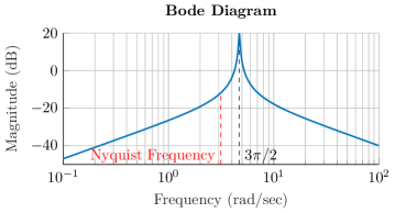
Figure 3: Weighting function $F(s)$ in Example IV.1

The response against the sinusoid $r(t)=\sin(3\pi/2)t$ is shown in Fig. 4 along with the delayed error, represented by the dashed line. Here we chose the upsampling factor $M=8$ and the delay $L=4h=4$.

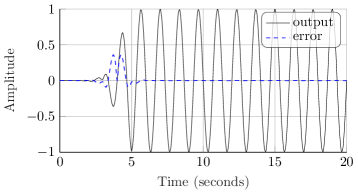
Figure 4: System output tracking $\sin(3\pi/2)t$ along with the delayed error

This figure clearly shows that the output tracks the reference input $\sin(3\pi/2)t$, which has the natural frequency greater than the Nyquist frequency $\pi$, and the output matches the given frequency $3\pi/2$. Note also that the output shows the delay of $4$ steps specified by the design specification. $\diamondsuit$

Figure 5: Discrete-time controller output

Figure 6: Poles of the controller

Fig. 6 shows the eigenvalues of the upsampled controller, i.e., those of $A_{d}$. There are poles at $\pm j$ corresponding to $e^{\pm 3\pi j/2}$—necessary to produce $\sin(3\pi/2)t$, along with $e^{\pm j\omega h/M}$ with $\omega=3\pi/2$, $M=8$, as discussed in Remark III.3.

Remark IV.2

For the choice of the design parameter $M$, there is a clear trade-off between the accuracy of the internal model (and the tracking output) and computational burden. For example, if we increase the upsampling factor $M$ in the example above, it is expected that the designed controller produces more accurate sinusoids compared with the one in Fig. 5, at the expense of computational cost. Generally speaking, our experience tells us that $M=8$ gives a suitable compromise.

One may also question if the above success of hypertracking is perhaps due to the relatively “low” tracking signal; but it has been shown that even a higher frequency signal of $\sin(5\pi/2)t$ can be well tracked [29].

Remark IV.3

As we noted, the delay length $L$ is a design parameter. By comparison with the case $L=0$, we easily see that a larger $L$ can generally provide more design freedom, but it is not necessarily true that a larger $L$ always leads to a better result. This is closely related to robustness, and will be discussed in detail in the subsequent Section V. See also [14] for the behavior as we increase $L$.

V Robustness

In this section we discuss the robustness condition for hypertracking/hyperrejection problems under the presence of plant fluctuations or reference/disturbance frequency variations.

The following theorem clarifies the crucial relationship between the tracking delay $L$ and robustness:

Theorem V.1

Consider the hypertracking problem in Fig. 1 with tracking/rejection signal $\sin\omega t$ and tracking delay $L=mh$. Under the condition of closed-loop stability, the closed-loop system Fig. 1 with tracking delay $L$ possesses an (approximate) internal model of this sinusoidal signal, (and hence robust (approximate) tracking) if and only if $L$ is an integer multiple of the period $2\pi/\omega$ of $\sin\omega t$.

Let us first give a brief argument on this fact. Recall Theorem III.2 on the transmission zeros of the closed-loop system, and the remark following it. The tracking signal here is $\sin\omega t$, and suppose also that $\pm j\omega$ is not an eigenvalue of the continuous-time plant $P$. Then, if tracking to $\sin\omega t$ is achieved, it means $\lambda=e^{j\omega h}$ should be an eigenvalue of $\overline{A_{d}}$, and, simultaneously, $e^{j\omega h/M}$ an eigenvalue of $A_{d}$ as noted there (Remark III.3). Hence with a proper choice of the hold device $H(\theta)=e^{j\omega\theta}$, the discrete-time controller $K(z)$ should work as an internal model for $\sin\omega t$. When the hold device is a fast zero-order hold on $[0,h/M]$ instead, the tracking becomes approximate.

Proof of Theorem V.1 We adopt the framework of [25] to place sampled-data systems into a continuous-time scheme with the identification of $z\leftrightarrow e^{hs}$. To be more specific, the finite Laplace transform over the period $[0,h)$

$${\bf L}[\phi](s):=\int_{0}^{h}\phi(t)e^{-st}dt$$

turns the discrete-time controller $K(z)$ into $K(e^{hs})$. With respect to this setting, the controller $K(e^{hs})$ is to receive a sampled signal

$$\sum_{k}e_{k}(0)e^{-khs}$$

which is the Laplace transform of the impulse train

$$\sum_{k}e_{k}(0)\delta_{kh},$$

where $\delta_{kh}$ is the delta distribution placed at point $kh$. The loop transfer operator then becomes $K(e^{hs}){\bf L}[H](s)P(s)$. Suppose for the moment that $H$ is the zero-order hold. Then ${\bf L}[H](s)=(e^{hs}-1)/se^{hs}$, and the loop transfer operator is expressible as a ratio of polynomials in $s$ and $e^{hs}$. (For a more detailed discussion, see [25, page 710].) Hence this falls into the category of pseudorational transfer functions [23, 24]. In fact, even when $H$ is not the zero-order hold, but is a compactly supported function on $[0,h)$, it is still pseudorational. They are generally expressible as ratios of entire functions of the complex variable $s$.

Consider the block diagram in Fig. 7. Suppose that the tracking signal is generated by $1/\alpha(s)$ where $\alpha(s)$ is a polynomial in $s$. In the present case, $\alpha(s)=s^{2}+\omega^{2}$. The forward-loop system is described by $D^{-1}(s)N(s)$, where $D$ and $N$ are entire functions of exponential type. If the tracking is achieved, then in the steady-state mode it is equivalent to Fig. 8. This is precisely in the scope of the situation considered in [25, Theorem 6.4]. Hence the asymptotic tracking implies that any signal generated by $\alpha^{-1}(s)$ must be contained in the response generated by $D^{-1}(s)$. This implies $\alpha(s)|D(s)$ [25, Theorem 6.4]. That is, the forward loop must contain $\alpha(s)$ as an internal model. If $\alpha(s)=s^{2}+\omega^{2}$ and if $P(s)$ does not contain $\alpha(s)$ in the denominator, then $\alpha(s)$ must be contained in the controller $K(z)$ in combination with the hold element $H(\theta)$.

Now let us return to the issue of the tracking delay $L$. As we noted, the current objective is to make $y(t)$ track the delayed signal $r(t-L)$, not $r(t)$. In other words, the argument above works ideally only for the case $L=0$. When $L$ is nonzero, our design seeks a controller that makes $r(t-L)-y(t)\rightarrow 0$ but $e(t)=r(t)-y(t)$ need not go to zero. However, if $r(t)=\sin\omega t$ and if $L$ is selected to be an integer multiple of the period $2\pi/\omega$ of $\sin\omega t$, then $\sin\omega(t-L)-y(t)\rightarrow 0$ also implies $e(t)\rightarrow 0$. Under this condition, we return to the situation discussed above, and $e(t)\rightarrow 0$ is guaranteed.

Hence the above argument works again, and $\alpha(s)|D(s)$, which means that $s^{2}+\omega^{2}$ must be included in the forward-loop as an internal model.

Conversely, if the above divisibility condition $(2\pi/\omega)|L$ does not hold, then the tracking $r(t-L)-y(t)\rightarrow 0$ does not guarantee $e(t)\rightarrow 0$. Indeed, $r(t-L)-y(t)\rightarrow 0$ and $e(t)=r(t)-y(t)\rightarrow 0$ hold simultaneously only when $(2\pi/\omega)|L$. Hence this is a necessary and sufficient condition for an internal model to be formed in the forward loop transfer operator. $\Box$

Figure 7: Generalized tracking configuration

Figure 8: Steady-state mode

Remark V.2

The above proof gives an argument for an ideal case where the internal model is given as a continuous-time system. While this is possible for some choice of a generalized hold $H(\theta)$ (see, for example [25], where $1/s$ can be generated in a combination of a suitable hold and a discrete-time controller), the internal model is not exact in the sampled-data context, in general. As we have seen in Remark III.3, the precise tracking is not achieved because of the finite resolution of the upsampling factor $M$, and the compensator cannot exactly generate the sinusoid $\sin\omega t$, but only approximately. However, as shown in [26], this error due to sample and hold approaches the continuous-time internal model as $M$ increases. Hence the proof above shows that the result should hold in the limiting case.

We give two suggestive examples. The nominal plant $P(s)$ is the same as (12):

$$P(s)=\frac{1}{s^{2}+2s+1}.$$

with the sampling time $h=1$, the upsampling factor $M=8$, and the delay length $L=4h=4$.

Example V.3

Consider the tracking problem to the signal $r(t)=\sin(4\pi/3)t$. We take the weighting function

$$F_{r}(s):=\frac{s}{s^{2}+0.01s+(4\pi/3)^{2}}.$$

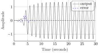
Figure 9: System output tracking $\sin(4\pi/3)t$ without disturbance

As Fig. 9 shows, this gives a fine tracking property. However, if we perturb the plant $P$ to $P+\Delta$, $\Delta(s)=0.05/(s+1)$, the resulting response exhibits a fairly large error as shown in Fig. 10, failing to show a robust tracking property. Note that the closed-loop system remains stable here.

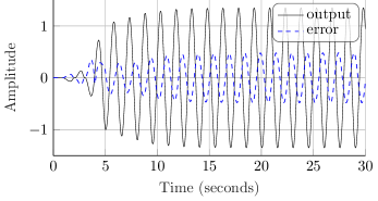
Figure 10: System output for the reference $\sin(4\pi/3)t$ under the additive perturbation $0.05/(s+1)$ to the plant

$\diamondsuit$

On the other hand, the following example exhibits quite a different behavior:

Example V.4

We take the same plant and simulation condition as in Example V.3, but with the tracking signal $r(t)=\sin(3\pi/2)t$. The result of robustness test for the plant perturbation $P\mapsto P+\Delta$, $\Delta(s)=0.1/(s+1)$ is given by Fig. 11.

In spite of the larger plant perturbation, the closed-loop system achieves a steady-state tracking.

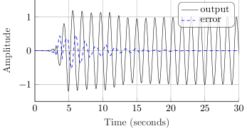
Figure 11: System output tracking $\sin(3\pi/2)t$ under the additive perturbation $0.1/(s+1)$ to the plant

$\diamondsuit$

In light of Theorem V.1, the difference of the above two is clear: In Example V.3, the period $2\pi/(4\pi/3)=3/2$ does not divide $L=4$ while in the latter Example V.4, $L=4$ is an integer multiple of $2\pi/(3\pi/2)=4/3$, thereby assuring robust tracking. We can also easily ensure that taking $L=6$ in Example V.3 will recover the robust tracking property as shown in Fig. 12.

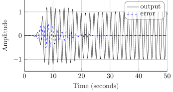
Figure 12: System output tracking $\sin(4\pi/3)t$ with $L=6$ under the additive perturbation $0.1/(s+1)$ to the plant

VI Miscellaneous Examples

We now give a few typical examples that can often arise in practical situations:

• hypertracking for multiple sinusoids above the Nyquist frequency;

• simultaneous tracking and disturbance rejection objectives;

• simple hypertracking for an unstable plant;

• hypertracking for a non-minimum phase plant.

In all the examples, the delay $L$ is chosen to be an integer multiple of the tracking/rejection frequency so that the robustness is guaranteed.

VI-A Hypertracking to multiple sinusoids

The following example shows a case where we have two tracking frequencies above the Nyquist frequency:

Example VI.1

(Hypertracking for multiple sinusoids) Let

$$P(s):=\frac{1}{s^{2}+2s+1}$$

with (normalized) sampling period $h=1$ (and hence the Nyquist frequency is $\pi$ [rad/sec].) We aim at tracking two sinusoids $\sin(5\pi/4)t+\sin(9\pi/4)t$, having natural frequencies above the Nyquist frequency. We set the upsampling factor $M=8$ and the delay $L=8$. The weighting function is chosen as

$$F(s):=\frac{s}{(s^{2}+0.01s+(5\pi/4)^{2})(s^{2}+0.01s+(9\pi/4)^{2})}$$

to have clear peaks at $5\pi/4$ and $9\pi/4.$ The result is shown in Fig. 13. We see that tracking is well achieved even for this multiple signal tracking.

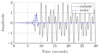
Figure 13: Hypertracking for multiple sinusoids $\sin(5\pi/4)t+\sin(9\pi/4)t$

$\diamondsuit$

VI-B Simultaneous tracking and disturbance rejection

We now consider the simultaneous tracking and disturbance rejection problem given in Fig. 1 where the disturbance $d$ is injected before the plant $P$. The generalized plant for the design is shown in Fig. 14 where $F_{r}$ and $F_{d}$ are the weights on the reference signal and the disturbance, respectively.

Figure 14: Generalized plant in the presence of input disturbance

Example VI.2

(Simultaneous tracking and rejection) Let $h=1,$ $M=8,$ $L=8$, and

$$P(s):=\frac{1}{s^{2}+2s+1}.$$

Our objective here is to track $r(t)=\sin\omega_{r}t$ while the system is subject to the disturbance $d(t)=\sin\omega_{d}t$.

We here set $\omega_{r}:=\pi/4$ and $\omega_{d}:=3\pi/2$; that is, the tracking frequency is low, and there is a high-frequency disturbance above the Nyquist frequency. We commonly encounter such a situation, e.g., in hard-disk drives, where the tracking frequency is below the Nyquist frequency but the disturbance is above it. We choose the weighting functions as

$$F_{r}(s):=\frac{s}{s^{2}+0.01s+\omega_{r}^{2}},\quad F_{d}(s):=\frac{s}{s^{2}+0.01s+\omega_{d}^{2}}.$$ (13)

The delayed output and the delayed error are shown in Fig. 15. This simultaneous tracking and disturbance rejection problem is reasonably well performed.

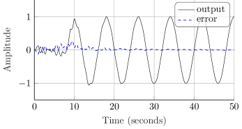
Figure 15: Delayed error against $\sin(\pi/4)t$ in the presence of the input disturbance $\sin(3\pi/2)t$

$\diamondsuit$

The following example treats a little more delicate case where the tracking and rejection signals are at the same frequency:

Example VI.3

(Simultaneous tracking and rejection of the same frequency) We now consider a more demanding case of tracking and rejecting the same sinusoid of $\sin(3\pi/2)t$ for the same plant as in Example VI.2. The weighting functions are set to be in the form (13) with $\omega_{r}=\omega_{d}=3\pi/2.$ The delayed output and the delayed error are shown in Fig. 16. While the response is somewhat slower, the result shows good tracking/rejection.

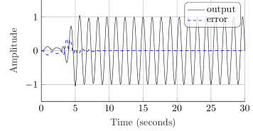
Figure 16: Delayed error against $\sin(3\pi/2)t$ in the presence of the input disturbance $\sin(3\pi/2)t$

$\diamondsuit$

Remark VI.4

It may be noted that the transfer operator from the disturbance to the output is not the complementary sensitivity function, but rather $P/(1+PC)$. Therefore, the classical trade-off between the sensitivity function and the complementary sensitivity function in a closed-loop system does not apply here. See also [21] for more details in multiple signal tracking and rejection, with a slightly different two-step design method.

VI-C Simple hypertracking for an unstable plant

We have so far considered only a stable and minimum-phase plant. We will now see that hypertracking (and hyperrejection) also works for unstable or non-minimum phase plants.

The following example shows a case for an unstable plant:

Example VI.5

(Hypertracking for an unstable plant) Take an unstable plant $P$:

$$P(s):=\frac{1}{(s-0.5)},$$

with $h=1,$ $M=8,$ $L=4,$ and the weighting

$$F(s)=\frac{s}{s^{2}+0.01s+(3\pi/2)^{2}}.$$

The delayed output and the delayed error against $\sin(3\pi/2t)$ are shown in Fig. 17. Again, hypertracking is well achieved for this case also.

Figure 17: Delayed tracking for $\sin(3\pi/2)t$ for an unstable plant

$\diamondsuit$

VI-D Simple hypertracking for a non-minimum phase plant

Finally, we give the following example dealing with a non-minimum phase plant.

Example VI.6

(Hypertracking for a non-minimum phase plant.) Take the following plant that has an unstable zero at $s=1$:

$$P(s):=\frac{s-1}{s^{2}+2s+1}.$$

The tracking frequency is $3\pi/2$ as before, and we take the weighting

$$F(s)=\frac{s}{s^{2}+0.01s+(3\pi/2)^{2}},$$

with the same $h=1,$ $M=8,$ and $L=4$ as above.

The delayed output and the delayed error are shown in Fig. 18. While there remain some errors, the overall tracking must be satisfactory.

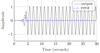
Figure 18: Delayed error against $\sin(3\pi/2)t$ for a non-minimum phase plant

$\diamondsuit$

VII Concluding remarks

We have proposed a new scheme (along with [29]) for tracking/rejection of signals that reside either beyond or below the Nyquist frequency. This has been made possible by introducing a suitable choice of signal weighting. When the tracking/rejection signal is above the Nyquist frequency, an appropriate choice allows us to control high-frequency intersample response.

We have also completely characterized robustness in this context. That is, the designed closed-loop system achieves robust tracking/rejection if and only if the tracking/rejection delay $L$ is an integer multiple of the periods of target signals (Theorem V.1). This leads to an interesting observation.

In general, when there is no feedback loop, i.e., in the case of a delayed signal reconstruction, a longer delay length is always advantageous; for example, in the signal reconstruction, the designed filter will approach an ideal filter as $L\rightarrow\infty$ [6]. In the present setting, however, a longer delay does not necessarily yield a desirable result in view of robustness. A delay incompatible with the target signal period can behave very poorly when there is a small amount of perturbations.

Multirate sampled-data control has been studied in the control literature: see, e.g., [2, 10, 12, 13]. However, the emphasis there is mainly on how one can obtain full information by multirate sampling of the output, thereby extending the capability of control. It is to be noted that we do not perform further sampling on the sampled output, and the basic sampling period remains intact for outputs. Upsampling is performed only on the side of the control signals, and we focus our attention on how it can enhance control capability. This is made possible by a proper choice of weighting on tracking/rejection signals.

References

- [1] B. D. O. Anderson and J. P. Keller, Discretization Techniques in Control Systems, Control and Dynamic Systems. Academic Press, New York, 1998.
- [2] M. Araki and K. Yamamoto, “Multivariable multirate sampled-data systems: state-space description, transfer characteristics, and Nyquist criterion,” IEEE Trans. Autom. Control, vol. AC-31, pp. 145–154, 1986.
- [3] T. Atsumi, “Disturbance suppression beyond Nyquist frequency in hard disk drives,” Mechatronics, vol. 20, no. 1, pp. 67–73, 2010.
- [4] B. Bamieh and J. B. Pearson, “A general framework for linear periodic systems with applications to sampled-data control,” IEEE Trans. Autom. Control, vol. 37, no. 4, pp. 418–435, 1992.
- [5] B. Bamieh, J. B. Pearson, B. A. Francis, and A. Tannenbaum, “A lifting technique for linear periodic systems with applications to sampled-data control,” Syst. Control Lett., vol. 17, no. 2, pp. 79–88, 1991.
- [6] T. Chen and B. A. Francis, “Design of multirate filter banks by opimization,” IEEE Trans. Signal Processing, vol. SP-43, pp. 2822–2830, 1995.
- [7] ——, Optimal Sampled-Data Control Systems. Springer, London, 1995.
- [8] N. J. Fliege, Multirate Digital Signal Processing. New York: John Wiley, 1994.
- [9] W. E. Frazier, “Metal additive manufacturing: A review,” J. Mater. Eng. Perform., vol. 23, no. 6, pp. 1917–1928, 2014.
- [10] T. Hagiwara and M. Araki, “Design of a stable state feedback controller based on the multirate sampling of the plant output,” IEEE Trans. Autom. Control, vol. 33, no. 9, pp. 812–819, 1988.
- [11] A. C. Kahane, L. Mirkin, and J. Z. Palmor, “Incorporating waveform constraints in optimal design of sampling and hold functions,” in Proc. 38th IEEE Conference on Decision and Control, 1999, pp. 3900–3905.
- [12] T. Mita and Y. Chida, “2-delay digital feedback control and its applications—avoiding the problem on unstable zeros,” SICE Transactions, vol. 24, no. 5, pp. 467–474, 1988.
- [13] T. Mita, Y. Chida, Y. Kaku, and H. Numasato, “Two-delay robust digital control and its applications-avoiding the problem on unstable limiting zeros,” IEEE Trans. Autom. Control, vol. 35, no. 8, pp. 962–970, 1990.
- [14] K. Y. Polyakov, E. N. Rosenwasser, and B. P. Lampe, “Design of optimal sampled-data tracking systems with preview,” in Proc. 4th IFAC Workshop on Time Delay Systems, 2003, pp. 327–332.
- [15] L. Qiu and T. Chen, “Multirate sampled-data systems: all suboptimal controllers and the minimum entropy controllers,” IEEE Trans. Autom. Control, vol. 44, pp. 537–550, 1999.
- [16] C. E. Shannon, “Communication in the presence of noise,” Proc. IRE, vol. 37, no. 1, pp. 10–21, 1949.
- [17] J. Tani, S. Mishra, and J. T. Wen, “Identification of fast-rate systems using slow-rate image sensor measurements,” IEEE/ASME Trans. Mechatronics, vol. 19, no. 4, pp. 1343–1351, 2014.
- [18] P. P. Vaidyanathan, Multirate Systems and Filter Banks. Prentice Hall, Englewood Cliffs, 1993.
- [19] P. G. Voulgaris, M. A. Dahleh, and L. Valavani, “ and optimal controllers for periodic and multirate systems,” Automatica, vol. 30, pp. 251–263, 1994.
- [20] H. Xiao, T. Jiang, and X. Chen, “Rejecting fast narrow-band disturbances with slow sensor feedback for quality beam steering in selective laser sintering,” Mechatronics, vol. 56, pp. 166–174, 2018.
- [21] K. Yamamoto, Y. Yamamoto, and M. Nagahara, “Simultaneous rejection of signals below and above the Nyquist frequency,” in Proc. 1st IEEE Conf. Control Tech. and Appl., 2017, pp. 1135–1139.
- [22] ——, “Hypertracking beyond the Nyquist frequency,” in Emerging Applications of Control and Systems Theory—A Festschrift in Honor of Mathukumalli Vidyasagar. Springer-Verlag, 2018, pp. 369–379.
- [23] Y. Yamamoto, “Pseudo-rational input/output maps and their realizations: a fractional representation approach to infinite-dimensional systems,” SIAM J. Contr. Optimiz., vol. 26, pp. 1415–1430, 1988.
- [24] ——, “Reachability of a class of infinite-dimensional linear systems: an external approach with applications to general neutral systems,” SIAM J. Contr. Optimiz., vol. 27, pp. 217–234, 1989.
- [25] ——, “A function space approach to sampled-data control systems and tracking problems,” IEEE Trans. Autom. Control, vol. AC-39, pp. 703–713, 1994.
- [26] Y. Yamamoto, A. G. Madievski, and B. D. O. Anderson, “Approximation of frequency response for sampled-data control systems,” Automatica, vol. 35, no. 4, pp. 729–734, 1999.
- [27] Y. Yamamoto and M. Nagahara, “Digital control,” Wiley Encyclopedia of Electrical and Electronics Engineering, 2018. [Online]. Available: https://onlinelibrary.wiley.com/doi/10.1002/047134608X.W1010.pub2
- [28] Y. Yamamoto, M. Nagahara, and P. P. Khargonekar, “Signal reconstruction via sampled-data control theory—beyond the Shannon paradigm,” IEEE Trans. Signal Processing, vol. SP-60, no. 2, pp. 613–625, 2012.
- [29] Y. Yamamoto, K. Yamamoto, and M. Nagahara, “Tracking to signals beyond the Nyquist frequency,” in Proc. 55th IEEE Conf. Decision and Control, 2016, pp. 4003–4008.
- [30] M. Zheng, L. Sun, and M. Tomizuka, “Multi-rate observer based sliding mode control with frequency shaping for vibration suppression beyond Nyquist frequency,” IFAC-PapersOnLine, vol. 49, pp. 13–18, 2016.