Balanced Subsampling for Big Data with Categorical Covariates

Abstract

The use and analysis of massive data are challenging due to the high storage and computational cost. Subsampling algorithms are popular to downsize the data volume and reduce the computational burden. Existing subsampling approaches focus on data with numerical covariates. Although big data with categorical covariates are frequently encountered in many disciplines, the subsampling plan has not been well established. In this paper, we propose a balanced subsampling approach for reducing data with categorical covariates. The selected subsample achieves a combinatorial balance among values of covariates and therefore enjoys three desired merits. First, a balanced subsample is nonsingular and thus allows the estimation of all parameters in ANOVA regression. Second, it provides the optimal parameter estimation in the sense of minimizing the generalized variance of the estimated parameters. Third, the model trained on a balanced subsample provides robust predictions in the sense of minimizing the worst-case prediction error. We demonstrate the usefulness of the balanced subsampling over existing data reduction methods in extensive simulation studies and a real-world application.

Keywords: ANOVA; $D$-optimality; Massive data; Orthogonal array; LASSO regression.

1 Introduction

In this “Big Data” era, massive volumes of data are collected from a variety of sources at an accelerating speed. Many of these data sets have the potential to contain important knowledge in various fields, yet the size of these data makes them difficult to manipulate. Although a number of scalable modeling techniques have emerged to accommodate big data, many tasks still suffer significant computational burden (Fan et al., 2014; Drovandi et al., 2017; Wang et al., 2016). Subsampling provides a feasible and principal way of converting big data into knowledge with available computational resources.

An intuitive subsampling idea is simple random sampling, that is, sampling the data points randomly at a uniform (equal) probability. This way provides a solution to the computational challenges of big data yet may miss important information contained in the data. In recent years, there has been a growing interest in the development of intelligent subsampling methods to preserve the information in big data. Most existing methods focus on data with numerical covariates and investigate the selection of a subsample that allows accurate establishment of statistical and machine learning models. For example, efficient subsampling algorithms have been developed for linear regression (Wang et al., 2019; Ma et al., 2015; Wang et al., 2021), generalized linear models (Wang et al., 2018; Ai et al., 2021; Cheng et al., 2020), quantile regression (Wang and Ma, 2021; Ai et al., 2021), nonparametric regression (Meng et al., 2020), Gaussian process modeling (He and Hung, 2022), and model free scenarios (Mak and Joseph, 2018; Shi and Tang, 2021; Song et al., 2022).

Big data with categorical covariates are frequently encountered in many scientific research areas (Huang et al., 2014; Zuccolotto et al., 2018; Johnson et al., 2018). Numerical covariates may also be binned to categorical ones for better modeling and interpretation (Kanda, 2013; Yu et al., 2022). ANOVA regression with the least squares estimator trained on the coded dummy variables might be the first choice for studying categorical covariates. For a full dataset with $N$ observations of $p$ categorical covariates, each with $q_{j}$ levels for $j=1,\ldots,p$, the required computing time for obtaining the least squares estimator is $O(N(\sum_{j=1}^{p}q_{j})^{2}+(\sum_{j=1}^{p}q_{j})^{3})$, which is $O(N(\sum_{j=1}^{p}q_{j})^{2})$ for a big $N$. The computation can be slow due to a large data volume and many levels of covariates. Moreover, when $p$ or some $q_{j}$’s are big, creating a high-dimensional problem, penalized least squares base-learner is necessary (Tibshirani, 1996; Zou and Hastie, 2005), and the computing time will multiply dramatically due to validation of hyperparameters. Analyzing a subsample instead of the full data is often inevitable. Despite the existing various studies on subsampling methods, they do not apply to data with categorical covariates, so that researchers have no choice but to use simple random subsamples, for example, see Maronna and Yohai (2000) and Yu et al. (2022).

In this paper, we propose a new subsampling approach, which we call balanced subsampling, for big data with categorical covariates. The selected subsample achieves a combinatorial balance between values (levels) of the covariates and therefore enjoys three desired merits. As pointed out by Maronna and Yohai (2000) and Koller and Stahel (2017), singular subsamples (or more accurately, subsamples with singular information matrices) can have an arbitrarily high probability for categorical covariates due to the coding system, so that the number of trials it takes to obtain a nonsingular simple random subsample may tend to infinity. To this end, the first merit of a balanced subsample is its nonsingularity, which is important because it allows the estimation of all parameters in ANOVA regression. Second, the accuracy of parameter estimation varies greatly across different subsamples even if they are all nonsingular. A balanced subsample provides the optimal parameter estimation in the sense of minimizing the generalized variance of the estimated parameters. Third, when the established model is used for prediction, the model trained on a balanced subsample provides robust predictions in the sense of minimizing the worst-case prediction error. For practical use, we develop an algorithm that sequentially selects data points from the full data to obtain a balanced subsample. For a large $N$ and a fixed subsample size $n$, the computational complexity of selecting and training a balanced subsample is as low as $O(Np)$, which dramatically saves the computation compared with training the full data. Moreover, the proposed method is suitable for distributed parallel computing to further accelerate the computation.

The remainder of the paper is organized as follows. In Section 2, we present the issues of simple random subsampling for data with categorical covariates, which motivates us to develop a new subsampling method. In Section 3, we propose the balanced subsampling method and use it to develop a computationally efficient algorithm for sequentially subsampling from big data. In Section 4, we examine the performance of the balanced subsampling through extensive simulations. In Section 5, we demonstrate the utility of using balanced subsamples in a real-world application. We offer concluding remarks in Section 6 and show the proof of technical results in the appendix.

2 Motivations

Let $(x_{1},y_{1}),\ldots,(x_{N},y_{N})$ denote the full data, where $x_{i}=(x_{i1},\ldots,x_{ip})^{T}$ consists of the values of $p$ categorical covariates, each with $q_{j}$ levels for $j=1,\ldots,p$, and $y_{i}$ is the corresponding response. Each covariate is coded with $q_{j}-1$ binary dummy variables. We consider the ANOVA regression:

$$y_{i}=\beta_{0}+\sum_{k=1}^{q_{1}-1}\beta_{1k}z_{i,1k}+\cdots+\sum_{k=1}^{q_{p}-1}\beta_{pk}z_{i,pk}+\varepsilon_{i},$$ (1)

where $z_{i,jk}$ is the value of the $k$th dummy variable for $x_{ij}$, $\beta_{jk}$ is its corresponding parameter to be estimated, and $\varepsilon_{i}$ is the independent random error with mean 0 and variance $\sigma^{2}$. Let $y=(y_{1},\ldots,y_{N})^{T}$, $z_{i}=(1,z_{i,11},\ldots,z_{i,1(q_{1}-1)},\ldots,z_{i,p1},\ldots,z_{i,p(q_{p}-1)})^{T}$, $Z=(z_{1},\ldots,z_{N})^{T}$, $\beta=(\beta_{0},\beta_{11},\ldots,\beta_{1(q_{1}-1)},\ldots,\beta_{p1},\ldots,\beta_{p(q_{p}-1)})^{T}$, and $\varepsilon=(\varepsilon_{1},\ldots,\varepsilon_{N})^{T}$. The matrix form of the model in (1) is given by

$$y=Z\beta+\varepsilon$$ (2)

where the ordinary least squares (OLS) estimator of $\beta$ is

$$\hat{\beta}=(Z^{T}Z)^{-1}(Z^{T}y).$$

Now consider taking a subsample of size $n$ from the full data. Denote the subsample by $(X_{s},y_{s})$ which contains data points $(x_{1}^{*},y_{1}^{*}),\ldots,(x_{n}^{*},y_{n}^{*})$ from the full data. The OLS estimator based on the subsample is given by

$$\hat{\beta}_{s}=(Z_{s}^{T}Z_{s})^{-1}(Z_{s}^{T}y_{s}),$$ (3)

where $Z_{s}=(z_{1}^{*},\ldots,z_{n}^{*})^{T}$ are the rows in $Z$ corresponding to points in $X_{s}$. We have three concerns regarding the subsample $X_{s}$.

2.1 Nonsingularity

The subsample should allow the estimation of all parameters in $\beta$, which is possible only if the information matrix of $X_{s}$, $M_{s}=Z_{s}^{T}Z_{s}$, is nonsingular. However, singular subsamples (subsamples with a singular information matrix) can have an arbitrarily high probability for categorical covariates, which can be seen from the following two toy examples.

Example 1.

Assume the full data contain a single categorical covariate with 2 repetitions of 5 levels, that is, $X=(1,1,2,2,3,3,4,4,5,5)^{T}$. Use dummy variables, then

$$Z=\left(\begin{array}[]{cccccccccc}1&1&1&1&1&1&1&1&1&1\\ 1&1&0&0&0&0&0&0&0&0\\ 0&0&1&1&0&0&0&0&0&0\\ 0&0&0&0&1&1&0&0&0&0\\ 0&0&0&0&0&0&1&1&0&0\\ \end{array}\right)^{T}.$$

Consider choosing a subsample $X_{s}$ with 5 points, then $M_{s}$ is nonsingular only if $X_{s}$ contains at least one observation of each level. Out of the $\binom{10}{5}=252$ possible subsamples, only $2^{5}$ of them are good in this way, and the probability of obtaining such a subsample with simple random sampling is $2^{5}/252=12.7\%$.

Example 2.

Suppose the full data have $N=1000$ points and $p=2$ covariates. We generate data from independent bivariate normal distribution with mean 0 and variance 1, divide the range of either covariates into 5 equal-sized intervals, and code the values according to which interval they fall. Then each covariate includes 5 levels and the two covariates have 25 possible pairs of levels. Figure 2 (top) shows the frequencies of pairs of levels for the two covariates. Now we select a subsample of size $n=25$. There are $\binom{1000}{25}\approx 10^{49}$ possible subsamples from simple random sampling. An exhaustive examination of all those subsamples is infeasible. Therefore, we randomly investigate $10^{5}$ of them, and only 4.81% of them have nonsingular information matrices. It is not easy to obtain a nonsingular subsample from simple random sampling.

2.2 Optimal estimation

Even for the nonsingular subsamples, the accuracy of parameter estimation varies greatly for different subsamples.

Example 3.

Consider the full data in Example 2. We generate the response variable $y$ through the model

$$y_{i}=1+z_{i,11}+\cdots+z_{i,14}+z_{i,21}+\cdots+z_{i,24}+\varepsilon_{i},$$ (4)

where $\varepsilon_{i}\sim N(0,1)$ for $i=1,\ldots,1000$. We repeatedly generate the response for $T=1000$ times. For each repetition, we train the model in (1) on each of the nonsingular subsamples and examine the empirical mean squared error:

$$\mbox{MSE}=T^{-1}\sum_{t=1}^{T}\|\hat{\beta}^{(t)}-\beta\|^{2},$$ (5)

where $\hat{\beta}^{(t)}$ is the OLS estimate of $\beta$ via a subsample in the $t$th repetition, $t=1,\ldots,1000$. Figure 1 (left) shows the histogram of $\log_{10}$(MSE) for all nonsingular subsamples. The MSE varies dramatically, with the minimum as low as $10^{0.85}=7.1$ achieved by only a couple of subsamples. Recall that we examined $10^{5}$ random subsamples, and only a couple of them allows the “optimal” estimation. It is very hard to obtain such “optimal” subsamples from simple random sampling.

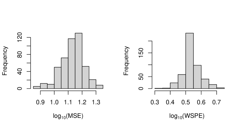
Figure 1: Histograms of $\log_{10}$(MSE) and $\log_{10}$(WSPE) of the trained model on each subsample with a nonsingular information.

2.3 Robust prediction

We hope the trained model on a subsample provides “robust” prediction, where the terminology “robust” can be understood in the sense of performing well in the worst-case scenario.

Example 4.

We continue Example 3 and examine the empirical worst-case squared prediction error (WSPE) for all nonsingular subsamples:

$$\mbox{WSPE}=\max_{x\in\mathcal{X}}\left\{T^{-1}\sum_{t=1}^{T}(y^{(t)}-z^{T}\hat{\beta}^{(t)})^{2}\right\}$$ (6)

where $\mathcal{X}$ includes all the 25 possible pairs of levels for the two covariates, and for any $x\in\mathcal{X}$, $z$ is the vector of its dummy variables, $y^{(t)}$ is the response in the $t$th repetition, and $\hat{\beta}^{(t)}$ is the OLS estimate of $\beta$ via a subsample, for $t=1,\ldots,1000$. Figure 1 (right) shows the histogram of $\log_{10}$(WSPE) for all the nonsingular subsamples. The minimum of WSPE is $10^{0.31}=2.0$ achieved by a single subsample, which is, again, almost impossible to obtain from simple random sampling.

3 Balanced Subsampling

In this section, we propose the balanced subsampling method and develop a computationally efficient algorithm to implement the method. The proposed method targets at the above three concerns and provides a subsample that is nonsingular and allows the optimal parameter estimation and robust prediction.

3.1 The method

We first consider the nonsingularity of a subsample and provide the following important result.

Theorem 1.

Let $\lambda_{\min}(M_{s})$ be the smallest eigenvalue of $M_{s}$. For a subsample $X_{s}$,

$$\lambda_{\min}(M_{s})\geq n\nu(1-f(X_{s}))$$

where $n$ is the subsample size of $X_{s}$, $\nu$ is a positive constant independent of $X_{s}$,

$$f(X_{s})=\sqrt{\sum_{j=1}^{p}\sum_{u=1}^{q_{j}}q_{j}^{2}\left[\frac{1}{q_{j}}-\frac{n_{j}(u)}{n}\right]^{2}+\sum_{j=1}^{p}\sum_{k=1,k\neq j}^{p}\sum_{u=1}^{q_{j}}\sum_{v=1}^{q_{k}}q_{j}q_{k}\left[\frac{1}{q_{j}q_{k}}-\frac{n_{jk}(u,v)}{n}\right]^{2}},$$ (7)

$n_{j}(u)$ is the number of times that the $u$th level of the $j$th covariate is observed in $X_{s}$, and $n_{jk}(u,v)$ is the number of times that the pair of levels $(u,v)$ is observed for the $j$th and $k$th covariates in $X_{s}$. Therefore, $M_{s}$ is nonsingular if $f(X_{s})<1$.

Theorem 1 indicates that we can search for the subsample that minimizes $f(X_{s})$ to ensure that the $M_{s}$ is nonsingular. By (7), $f(X_{s})$ has two critical components: (a) $f_{j}=\sum_{u=1}^{q_{j}}[1/q_{j}-n_{j}(u)/n]^{2}$ that measures the balance of levels for the $j$th covariate, and (b) $f_{jk}=\sum_{u=1}^{q_{j}}\sum_{v=1}^{q_{k}}[1/(q_{j}q_{k})-n_{jk}(u,v)/n]^{2}$ that measures the balance of level combinations for the $j$th and $k$th covariates. Clearly, if $f_{j}=0$, all levels of the $j$th covariate are observed the same number of times in $X_{s}$ so that they achieve the perfect balance; if $f_{jk}=0$, all pairs of levels for the $j$th and $k$th covariates are observed the same number of times in $X_{s}$. Such balance is called combinatorial orthogonality, and a matrix possessing combinatorial orthogonality is called an orthogonal array.

Generally, an orthogonal array of strength $t$ is a matrix where entries of each column of the matrix come from a fixed finite set of $q_{j}$ levels for $j=1,\ldots,p$, arranged in such a way that all ordered $t$-tuples of levels appear equally often in every selection of $t$ columns of the matrix. The $t$ is called strength of the orthogonal array. Readers are referred to Hedayat et al. (1999) for a comprehensive introduction of orthogonal arrays. Here is an example of orthogonal array with $p=3$ covariates, each of which has 3 levels, and strength $t=2$:

$$\left(\begin{array}[]{ccccccccc}1&1&1&2&2&2&3&3&3\\ 1&2&3&1&2&3&1&2&3\\ 1&2&3&2&3&1&3&1&2\\ \end{array}\right)^{T}.$$

Each pair of levels in any two columns of the orthogonal array appears once. Clearly, we have the following lemma.

Lemma 1.

A subsample $X_{s}$ forms an orthogonal array of strength two if and only if $f(X_{s})=0$.

Now we show that the subsample minimizing $f(X_{s})$ also allows the optimal estimation of parameters. To see this, note that $\hat{\beta}_{s}$ in (3) is an unbiased estimator of $\beta$ with

$$\mbox{Var}(\hat{\beta}_{s})=\sigma^{2}M_{s}^{-1}=\sigma^{2}(Z_{s}^{T}Z_{s})^{-1}.$$ (8)

The $\mbox{Var}(\hat{\beta}_{s})$ is a function of $X_{s}$ (in the form of $Z_{s}$), which indicates again that the subsampling strategy is critical in reducing the variance of $\hat{\beta}_{s}$. To minimize $\mbox{Var}(\hat{\beta}_{s})$, we seek the $X_{s}$ which, in some sense, minimizes $M_{s}^{-1}$. This is typically done, in experimental design strategy, by minimizing an optimality function $\psi(M_{s}^{-1})$ of the matrix $M_{s}^{-1}$ (Kiefer, 1959; Atkinson et al., 2007). A common choice for $\psi$ is the determinant, which is akin to the criterion of $D$-optimality for the selection of optimal experimental designs.

Theorem 2.

A subsample $X_{s}$ is $D$-optimal for the model in (1) if $f(X_{s})=0$.

Cheng (1980) showed that an orthogonal array of strength two is universally optimal, i.e., optimal under a wide variety of criteria by minimizing the sum of a convex function of coefficient matrices for the reduced normal equations. However, Cheng’s result does not apply to dummy coding system, so that his result does not include Theorem 2. To the best of our knowledge, Theorem 2 originally shows the optimality of orthogonal arrays for the commonly used dummy coding for categorical covariates.

Next we show that minimizing $f(X_{s})$ also allows robust prediction, that is, the model (1) trained on the subsample performs well for the worst-case scenario. Let $\mathcal{X}$ denote the set of all possible level combinations of covariates, that is, $\mathcal{X}=\{x=(x_{1},\ldots,x_{p}):x_{j}=1,\ldots,q_{j},j=1,\ldots,p\}$, then $\#\mathcal{X}=\prod_{j=1}^{p}q_{j}$. For any $x\in\mathcal{X}$, let $z$ be the coded vector of $x$ and $Y$ the random variable of its response. The following theorem shows that the WSPE, which is given by $\max_{x\in\mathcal{X}}E[(Y-z^{T}\hat{\beta}_{s})^{2}|X_{s}]$, is minimized when $f(X_{s})=0$.

Theorem 3.

Let $Q=1+\sum_{j=1}^{p}(q_{j}-1)$. For a subsample $X_{s}$ of size $n$,

$$\max_{x\in\mathcal{X}}E[(Y-z^{T}\hat{\beta}_{s})^{2}|X_{s}]\geq\sigma^{2}+Q/n.$$ (9)

The equality in (9) holds if $f(X_{s})=0$.

Theorems 1–3 indicate that $f(X_{s})=0$ ensures model estimability as well as optimal estimation and robust prediction. Considering that a full dataset may generally do not contain a subset with exact zero $f(X_{s})$, the objective of the balanced subsampling is to achieve an approximate balance via the optimization problem:

$$X_{s}^{*} = \arg\min_{X_{s}\subseteq X}f(X_{s})$$

$$s.t. X_{s}\mbox{ contains }n\mbox{ points.}$$

The optimization problem in (3.1) is not easy to solve. The computation of $f(X_{s})$ requires the examination of balance for every single covariate and every pair of covariates in $X_{s}$, so it requires $O(np^{2})$ operations to compute $f(X_{s})$ for any $X_{s}$. In addition, exhaustive search for all possible $X_{s}$ requires $O(N^{n})$ operations, making it infeasible for even moderate sizes of the full data. There are many types of algorithms for finding optimal designs and among them, exchange algorithms are among the most popular. For the reasons argued in Wang et al. (2021), these algorithms are cumbersome in solving the subsampling problem in (3.1). We will propose a sequential selection algorithm to efficiently select subsample points.

3.2 A sequential algorithm

The following result is critical in developing the algorithm.

Theorem 4.

For a subsample $X_{s}=(x_{ij}^{*})$, $i=1,\ldots,n$ and $j=1,\ldots,p$,

$$f^{2}(X_{s})=n^{-2}\sum_{1\leq i<l\leq n}[\delta(x_{i}^{*},x_{l}^{*})]^{2}+C,$$ (11)

where

$$\delta(x_{i}^{*},x_{l}^{*})=\sum_{j=1}^{p}q_{j}\delta_{1}(x_{ij}^{*},x_{lj}^{*}),$$ (12)

$\delta_{1}(x_{ij}^{*},x_{lj}^{*})$ is 1 if $x_{ij}^{*}=x_{lj}^{*}$ and 0 otherwise, and $C=n^{-1}(\sum_{j=1}^{p}q_{j})^{2}+p-\sum_{j=1}^{p}q_{j}-p^{2}$.

By Theorem 4, the optimization in (3.1) can be achieved by minimizing $\sum_{1\leq i<l\leq n}[\delta(x_{i}^{*},x_{l}^{*})]^{2}$. To select an $n$-point subsample, we start with a random point $x_{1}^{*}$ and select $x_{2}^{*},\ldots,x_{n}^{*}$ sequentially. Suppose we have already selected $m$ points, then the $(m+1)$th point is selected by

$$x_{m+1}^{*}=\arg\min_{x}~{}\left\{\sum_{i=1}^{m-1}\sum_{l=i+1}^{m}[\delta(x_{i}^{*},x_{l}^{*})]^{2}+\sum_{i=1}^{m}[\delta(x_{i}^{*},x)]^{2}\right\}\\ =\arg\min_{x}\Delta(x)$$

where

$$\Delta(x)=\sum_{i=1}^{m}[\delta(x_{i}^{*},x)]^{2},$$ (13)

and the minimization is over $x\in X\backslash\{x_{1}^{*},\ldots,x_{m}^{*}\}$. Since

$$\Delta(x)=\sum_{i=1}^{m-1}[\delta(x_{i}^{*},x)]^{2}+[\delta(x_{m}^{*},x)]^{2},$$

we only need to compute $\delta(x_{m}^{*},x)$ to update $\Delta(x)$ in the $(m+1)$th iteration so that the computational complexity is $O(Np)$. Algorithm 1 summarizes this sequential selection algorithm.

Algorithm 1 Balanced Subsampling (Sequential Selection)

  Input: a sample (dataset) $X$, a required subsample size $n$Output: a subsample $X_{s}$

  Set $m=1$ and randomly select $x_{1}^{*}$ from $X$

  for each $x\in X\backslash\{x_{1}^{*}\}$ do

     Compute $\Delta(x)$ via (13)

  end for

  while $m<n$ do

     Find $x_{m+1}^{*}=\arg\min_{x}\Delta(x)$ and include $x_{m+1}^{*}$ in $X_{s}$

     for each $x\in X\backslash\{x_{1}^{*},\ldots,x_{m+1}^{*}\}$ do

        Update $\Delta(x)\leftarrow\Delta(x)+[\delta(x_{m+1}^{*},x)]^{2}$

     end for

     $m\leftarrow m+1$

  end while

Example 5.

We continue the toy Examples 2–4 to illustrate the proposed balanced subsampling algorithms and show its usefulness. The full dataset is generated in Example 2. We select subsamples of size $n=25$ by three methods: simple random sampling (denoted as UNI to be consistent with literature since it uses a uniform weight for all observations), information based optimal subdata selection (IBOSS, Wang et al. (2019)), and the balanced subsampling implemented in Algorithm 1. Figure 2 shows the frequencies of possible pairs of levels for the two covariates in the full data (top) and the selected subsamples (bottom). UNI chooses points completely at random thus misses many pairs of levels. IBOSS is applied on the coded dummy variables and cannot provide better balance than UNI. Balanced subsampling selects a perfectly balanced subsample in which all 25 pairs are selected exactly once. We further consider different subsample sizes $n=25,50,100,250$, generate the response variable through the model in (4) (as in Examples 3 and 4), and examine the proportions of nonsingular information matrices, the empirical MSE in (5), and the empirical WSPE in (6), for all the selected subsamples, shown in Figure 3. The balanced subsamples always significantly outperform other approaches for any subsample size due to its balance on levels of covariates. Specifically, a balanced subsample almost always allows the estimation of the model. Increasing the subsample size may enhance the nonsingularity of UNI and IBOSS subsamples, but they still provide much worse parameter estimation and response prediction than a balanced subsample. It is interesting to note that the balanced subsample with 25 runs provides an even smaller MSE and WSPE than the best subsample searched from $10^{5}$ UNI subsamples in Examples 3 and 4. It is almost impossible to obtain a subsample from simple random sampling to be as good as the balanced subsample.

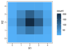
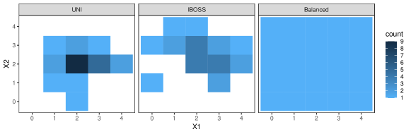
Figure 2: The full data (top) and subsamples (bottom) selected by different methods.

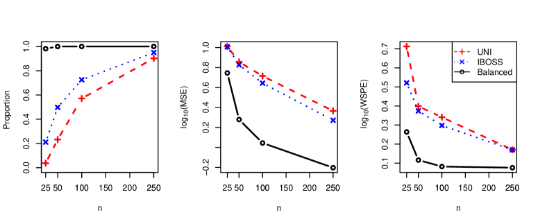
Figure 3: The proportions of nonsingular subsamples (left), MSEs of estimated parameters (middle), and WSPEs (right) for different subsampling methods in Example 5.

4 Simulation studies

We conduct simulation studies to assess merits of the balanced subsampling method relative to existing subsampling schemes. Consider $p=20$ covariates each with $q_{j}=j+1$ levels for $j=1,\ldots,p$. We generate values of the covariates under three structures:

• Covariates are independent, and each follows a discrete uniform distribution with $q_{j}$ levels.

• Covariates are independent, and for each covariate, the $q_{j}$ levels have probabilities proportional to $1,\ldots,q_{j}$.

• Generate each point $x_{i}$ from multivariate normal distribution: $x_{i}\sim N(0,\Sigma)$ with

  $$\Sigma=\left(0.5^{\xi(j,k)}\right),$$ (14)

  where $\xi(j,k)$ is equal to 0 if $j=k$ and 1 otherwise. Discretize $[-3,3]$ to $q_{j}$ intervals of equal length, and let $x_{ij}=u$ if $x_{ij}$ falls into the $u$th interval. Let $x_{ij}=1$ if $x_{ij}<-3$ and $x_{ij}=q_{j}$ if $x_{ij}>3$.

The response data are generated from the linear model in (1) with the true value of $\beta$ being a vector of unity and $\sigma=1$. The simulation is repeated $T=200$ times. We investigate four settings of the full data size $N=5\times 10^{3},10^{4},10^{5},$ and $10^{6}$ and two settings of the subsample size $n=500$ and 2000. Three subsampling approaches, UNI, IBOSS, and the balanced subsampling, are evaluated by comparing the proportions of nonsingular subsamples, MSEs (5), and WSPEs (6), with plots shown in Figures 4–6.

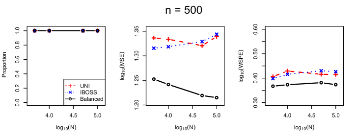
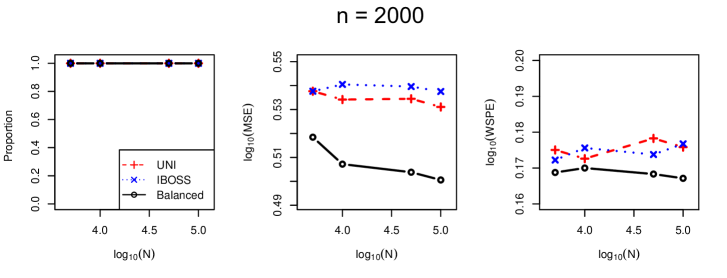
Figure 4: The proportions of nonsingular subsamples (left), MSEs of estimated parameters (middle), and WSPEs (right) for different subsampling methods for covariates in Case 1.

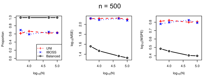
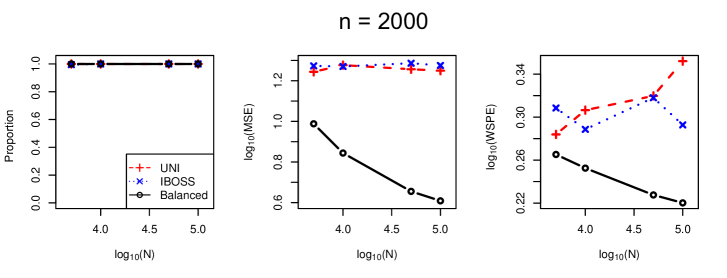
Figure 5: The proportions of nonsingular subsamples (left), MSEs of estimated parameters (middle), and WSPEs (right) for different subsampling methods for covariates in Case 2.

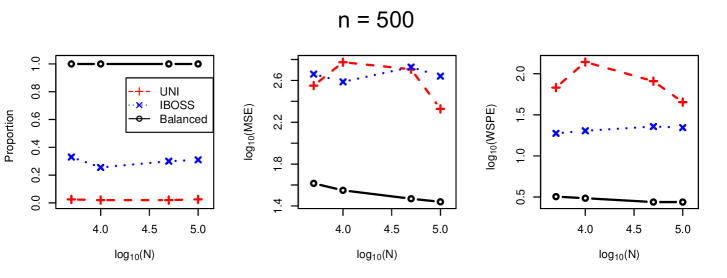
Figure 6: The proportions of nonsingular subsamples (left), MSEs of estimated parameters (middle), and WSPEs (right) for different subsampling methods for covariates in Case 3.

Figure 4 compares the subsampling methods for the full data generated in Case 1 where covariates have almost balanced levels. In this case, all subsamples are nonsingular and allow the estimates of all parameters. Even so, the balanced subsamples consistently provide more accurate parameter estimation and slightly better prediction than the UNI and IBOSS methods. Figure 5 plots results for Case 2 where levels of covariates are unbalanced, which is typically the case in real practice. We observe that, when the subsample size is $n=500$, only around 60% of UNI and IBOSS subsamples are nonsingular, while all balanced subsamples are nonsingular. Increasing the subsample size to $n=2000$ may improve the proportions of nonsingularity for the UNI and IBOSS methods, but the estimation and prediction obtained from those subsamples are still much worse than the balanced subsamples. More importantly, the MSEs and WSPEs from the balanced subsamples decrease fast as the full data size $N$ increases, even though the subsample size is fixed at $n=500$ or 2000. This trend demonstrates that the balanced subsampling extracts more information from the full data when the full data size increases. Note that IBOSS has this nice property for continuous covariates (Wang et al., 2019), but not for categorical covariates because of the high association between dummy variables. Figure 6 examines Case 3 where covariates are correlated in the full data. For $n=500$, almost all UNI subsamples are singular and only less than 40% of IBOSS subsamples are nonsingular. For either setting of the subsample size, we observe a greater superiority of the balanced subsamples and the decreasing trend of MSEs and WSPEs as the full data size increases. This is because the balanced subsamples have reduced correlation and enhanced combinatorial orthogonality between covariates, which helps reduce the collinearity between covariates and therefore allows more accurate estimate of parameters.

5 Real data applications

We consider the application to an online store offering clothing for pregnant women. The data are from five months of 2008 and include, among others, product category (4 levels), product code (217 levels), color (14 levels), model photography (2 levels), location of the photo on the page (6 levels), page number (5 levels), country of origin of the IP address of customers clicking the page (47 levels), month (5 levels), and product price in US dollars (continuous). The data contain more covariates to study the behavior patterns of customers. We are only using the above covariates to predict the product price and demonstrate the superiority of balanced subsamples. Further information on the dataset can be found in Łapczyński and Białowąs (2013).

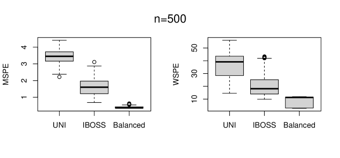
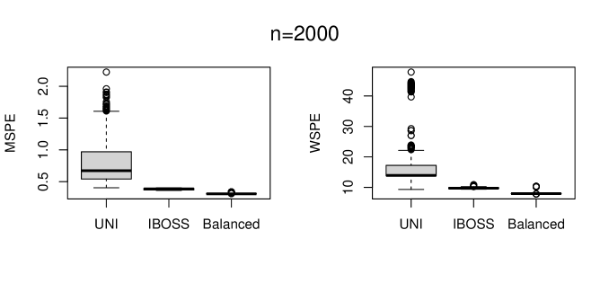
Figure 7: The MSPEs and WSPEs over the full data for different subsampling methods with $n=500$ (top) and 2000 (bottom).

The full dataset has $n=165,474$ data points. All covariates are categorical and are coded to dummy variables, which results 293 dummy variables in total (intercept included). We consider subsample sizes $n=500$ and $2000$, and select subsamples from the data with different methods. With such a number of dummy variables, we use LASSO regression (Tibshirani, 1996) to select important ones and train a predictive model. On each subsample, a LASSO regression model is trained via the R package “glmnet" (Friedman et al., 2010) with the parameter $\lambda$ selected by cross validation. We do 200 repetitions of this process and plot the MSPE (mean squared prediction error) and WSPE of the trained models over the full data in Figure 7. The balanced subsamples always allow much better predictions than UNI and IBOSS subsamples. Specifically, UNI subsamples provide the worst prediction of the full data. They select dramatically different points and give significantly different predictions, so their performance is not stable at all. IBOSS subsamples, by contrast, are more stable at a better performance because their subsamples are deterministic and covariates achieve better balance. The balanced subsamples always perform the best at both settings of the subsample size.

We further consider the saving on computation time. A LASSO regression on the full dataset takes around 50 second to run. Selecting a balanced subsample of size $n=500$ plus running LASSO regression on the subsample only takes 3 seconds. All computations are carried out on a laptop running Windows 11 Pro with an Intel Core i7-12700H processor and 32GB memory. Training the balanced subsample greatly accelerates the computation.

6 Discussion

In this paper, we proposed the balanced subsampling method for big data with categorical covariates. The selected subsample achieves a balance among levels of covariates, maximizing the overall information provided by the subsample. A balanced subsample is typically nonsingular and allows more accurate parameter estimation and prediction. Simulations and real-world application confirm the improved performance of the subsample selected by the balanced subsampling over other available subsampling methods. It should be noted that although this paper assumes binary dummy variables for coding the categorical covariates in ANOVA regression, all theoretical results work if any nonsingular coding system (for example, an orthogonal coding framework such as the orthogonal polynomial) is used for coding the covariates. The superiority of a balanced subsample does not depend on the coding system.

The balanced subsampling can be combined with robust regression, such as the S estimator, to enhance the robustness of the trained model to possible outliers. The training of the estimator involves repeatedly selecting small and nonsingular subsamples from the full data, which, as discussed in this paper and in (Koller and Stahel, 2017), is infeasible via simple random sampling. The randomness and nonsingularity of balanced subsamples make them applicable to training such estimators, although their performance for this purpose requires further study.

Though the proposed balanced subsampling is focused on big data with categorical covariates, it can be modified and generalized to select subsamples with numerical or mixed-type covariates. To do so, we may discretize the numerical covariates and apply Algorithm 1 to the discretized data. The selected subsample will cover the region of the full data evenly and uniformly, and therefore promote a fair study and robust prediction over the region. We will report our findings and results in a separate paper.

Appendix: Proofs

Recall that $\mathcal{X}$ denotes the set of all possible level combinations of covariates, that is, $\mathcal{X}=\{x=(x_{1},\ldots,x_{p}):x_{j}=1,\ldots,q_{j},j=1,\ldots,p\}$. Let $\mathcal{N}=\#\mathcal{X}=\prod_{j=1}^{p}q_{j}$. Let $\mathcal{Z}$ be the matrix of dummy variables for $\mathcal{X}$ and $C$ be the coded matrix for $\mathcal{X}$ via orthonormal contrasts with $C^{T}C=\mathcal{N}I$ (Cheng and Ye, 2004; Wang and Xu, 2022), where $I$ is a conformable identity matrix. Then there exists a transformation matrix $P$ such that $\mathcal{Z}=CP$. Because both $\mathcal{Z}$ and $C$ have full column ranks, so $P$ is nonsingular. Clearly, rows of $Z_{s}$ come from rows of $\mathcal{Z}$, so $Z_{s}=C_{s}P$ and $M_{s}=P^{T}C_{s}^{T}C_{s}P$, where rows of $C_{s}$ are from the corresponding rows of $C$.

Proof of Theorem 1.

Since $M_{s}=P^{T}C_{s}^{T}C_{s}P$, then

$$\lambda_{\min}(M_{s})=\lambda_{\min}(P^{T}C_{s}^{T}C_{s}P)\geq\lambda_{\min}(P^{T}P)\lambda_{\min}(C_{s}^{T}C_{s})=\nu\lambda_{\min}(C_{s}^{T}C_{s}),$$ (15)

where $\nu=\lambda_{\min}(P^{T}P)>0$. Let $\tilde{C}=I-C_{s}^{T}C_{s}/n=C^{T}C/\mathcal{N}-C_{s}^{T}C_{s}/n$, then

$$\tilde{C}=\left(\begin{array}[]{ccccc}0&C_{1}^{T}&C_{2}^{T}&\cdots&C_{p}^{T}\\ C_{1}&C_{11}&C_{12}^{T}&\cdots&C_{1p}^{T}\\ C_{2}&C_{12}&C_{22}&\cdots&C_{2p}^{T}\\ \vdots&\vdots&\vdots&\ddots&\vdots\\ C_{p}&C_{1p}&C_{2p}&\cdots&C_{pp}\\ \end{array}\right)$$

where $C_{j}$ is a $(q_{j}-1)$-vector with the $l$th entry $\sum_{u=1}^{q_{j}}[q_{j}^{-1}-n_{j}(u)/n]c_{jl}(u)=\sum_{u=1}^{q_{j}}[q_{j}^{-1}-n_{j}(u)/n]c_{jl}(u)c_{j0}(u)$ with $c_{j0}(u)=1$, $C_{jj}$ is a $(q_{j}-1)\times(q_{j}-1)$ matrix with the $(l,m)$th entry $\sum_{u=1}^{q_{j}}[q_{j}^{-1}-n_{j}(u)/n]c_{jl}(u)c_{jm}(u)$, $C_{jk}$ is a $(q_{j}-1)\times(q_{k}-1)$ matrix with the $(l,m)$th entry $\sum_{u=1}^{q_{j}}\sum_{v=1}^{q_{k}}[(q_{j}q_{k})^{-1}-n_{jk}(u,v)/n]c_{jl}(u)c_{km}(v)$, and $c_{jl}(u)$ is the coded value for the $l$th component of the $j$th covariate at level $u$. We have

$$\lambda_{\max}(\tilde{C})\leq\|\tilde{C}\|_{F}=\sqrt{f_{1}+f_{2}}$$

where $\|\cdot\|_{F}$ denotes the Frobenius norm and

$$f_{1} = \sum_{j=1}^{p}\sum_{l=0}^{q_{j}-1}\sum_{m=0}^{q_{j}-1}\sum_{u=1}^{q_{j}}\left[\frac{1}{q_{j}}-\frac{n_{j}(u)}{n}\right]^{2}c_{jl}^{2}(u)c_{jm}^{2}(u)$$

$$f_{2} = \sum_{j=1}^{p}\sum_{k=1,k\neq j}^{p}\sum_{l=1}^{q_{j}-1}\sum_{m=1}^{q_{k}-1}\sum_{u=1}^{q_{j}}\sum_{v=1}^{q_{k}}\left[\frac{1}{q_{j}q_{k}}-\frac{n_{jk}(u,v)}{n}\right]^{2}c_{jl}^{2}(u)c_{km}^{2}(v).$$

Because $\sum_{l=0}^{q_{j}-1}\sum_{m=0}^{q_{j}-1}c_{jl}^{2}(u)c_{jm}^{2}(u)\leq q_{j}^{2}$ and $\sum_{l=1}^{q_{j}-1}\sum_{m=1}^{q_{k}-1}c_{jl}^{2}(u)c_{km}^{2}(v)\leq q_{j}q_{k}$ for any $j,k$ and $u,v$, then

$$\lambda_{\max}(\tilde{C}) \leq \sqrt{\sum_{j=1}^{p}\sum_{u=1}^{q_{j}}q_{j}^{2}\left[\frac{1}{q_{j}}-\frac{n_{j}(u)}{n}\right]^{2}+\sum_{j=1}^{p}\sum_{k=1,k\neq j}^{p}\sum_{u=1}^{q_{j}}\sum_{v=1}^{q_{k}}q_{j}q_{k}\left[\frac{1}{q_{j}q_{k}}-\frac{n_{jk}(u,v)}{n}\right]^{2}}$$

$$= f(X_{s}).$$

Since $C_{s}^{T}C_{s}=n(I-\tilde{C})$, $\lambda_{\min}(C_{s}^{T}C_{s})=n(1-\lambda_{\max}(\tilde{C}))\geq n(1-f(X_{s}))$. Then by (15), $\lambda_{\min}(M_{s})\geq n\nu(1-f(X_{s})).$ $\Box$

Proof of Theorem 2.

Since $M_{s}=P^{T}C_{s}^{T}C_{s}P$, where $P$ is a $Q\times Q$ transformation matrix with $Q=1+\sum_{j=1}^{p}(q_{j}-1)$, then

$$\det(M_{s})=\det(P^{T}C_{s}^{T}C_{s}P)=\det(P)^{2}\det(C_{s}^{T}C_{s}).$$

Because $P$ is independent from the selection of $Z_{s}$, we only need to consider $\det(C_{s}^{T}C_{s})$:

$$\det(C_{s}^{T}C_{s}) = \prod_{j=1}^{Q}\lambda_{j}(C_{s}^{T}C_{s})$$ (16)

$$\leq \left\{\frac{\sum_{j=1}^{Q}\lambda_{j}(C_{s}^{T}C_{s})}{Q}\right\}^{Q}$$

$$= \left\{\frac{\mbox{tr}(C_{s}^{T}C_{s})}{Q}\right\}^{Q}$$

$$= \left\{\frac{n+\sum_{j=1}^{p}\sum_{l=1}^{q_{j}-1}\sum_{i=1}^{n}c_{i,jl}^{2}}{Q}\right\}^{Q}$$

$$= n^{Q},$$

where $\lambda_{j}(C_{s}^{T}C_{s})$’s for $j=0,1,\ldots,Q$ are eigenvalues of $C_{s}^{T}C_{s}$, $c_{i,jl}^{2}$ is the coded value for the $i$th observation in $Z_{s}$ of the $l$th component of the $j$ covariate, and the last equation holds because $1+\sum_{l=1}^{q_{j}-1}c_{i,jl}^{2}=q_{j}$ for any $i$ and $j$. If $f(X_{s})=0$, $X_{s}$ forms an orthogonal array and $C_{s}^{T}C_{s}=nI$, then $\det(C_{s}^{T}C_{s})=n^{Q}$. This completes the proof. $\Box$

Proof of Theorem 3.

We have

$$E[(Y-z^{T}\hat{\beta}_{s})^{2}|X_{s}]=E[(Y-z^{T}\beta)^{2}]+E[(z^{T}\beta-z^{T}\hat{\beta}_{s})^{2}|X_{s}]=\sigma^{2}+z^{T}M_{s}^{-1}z$$

and

$$\sum_{x\in\mathcal{X}}z^{T}M_{s}^{-1}z = \mbox{tr}(\mathcal{Z}M_{s}^{-1}\mathcal{Z}^{T})=\mbox{tr}\{\mathcal{Z^{T}Z}M_{s}^{-1}\}=\mbox{tr}\{P^{T}C^{T}CP(P^{T}C_{s}^{T}C_{s}P)^{-1}\}$$

$$= \mbox{tr}\{C^{T}C(C_{s}^{T}C_{s})^{-1}\}=\mathcal{N}\mbox{tr}\{(C_{s}^{T}C_{s})^{-1}\}\geq\mathcal{N}Q^{2}/\mbox{tr}(C_{s}^{T}C_{s})=\mathcal{N}Q/n,$$

where the last equation holds because $\mbox{tr}(C_{s}^{T}C_{s})=nQ$ following (16) and (Proof of Theorem 2.). Therefore, $\max_{x\in\mathcal{X}}z^{T}M_{s}^{-1}z\geq Q/n$ and $\max_{x\in\mathcal{X}}E[(Y-z^{T}\hat{\beta}_{s})^{2}|X_{s}]\geq\sigma^{2}+Q/n.$ On the other hand, when $f(X_{s})=0$, $X_{s}$ is balanced, and then for any $z$, $z^{T}M_{s}^{-1}z=z^{T}P^{T}Pz/n=\|Pz\|_{2}^{2}/n$. Note that $Pz$ is a row vector of $C$. The sum of squares of the $i$th row of $C$ is $(1+\sum_{j=1}^{p}\sum_{l=1}^{q_{j}-1}c_{i,jl}^{2})/n=(1+\sum_{j=1}^{p}(q_{j}-1))/n=Q/n$. Therefore, $z^{T}M_{s}^{-1}z=Q/n$ and $E[(Y-z^{T}\hat{\beta}_{s})^{2}|X_{s}]=\sigma^{2}+Q/n.$ This completes the proof. $\Box$

Proof of Theorem 4.

For a subsample $X_{s}=(x_{ij}^{*})$, it can be verified that $\sum_{u=1}^{q_{j}}n_{j}(u)=n$, $\sum_{u=1}^{q_{j}}\sum_{v=1}^{q_{k}}n_{jk}(u,v)=n$, and $\sum_{i=1}^{n}\sum_{l=1}^{n}\delta_{1}(x_{ij}^{*},x_{lj}^{*})\delta_{1}(x_{ik}^{*},x_{lk}^{*})=\sum_{u=1}^{q_{j}}\sum_{v=1}^{q_{k}}n_{jk}(u,v)^{2}$ for any $j,k=1,\ldots,p.$ Then

$$f^{2}(X_{s})$$

$$= \sum_{j=1}^{p}\sum_{u=1}^{q_{j}}\left(1-\frac{2q_{j}n_{j}(u)}{n}+\frac{q_{j}^{2}n_{j}(u)^{2}}{n^{2}}\right)+\sum_{j=1}^{p}\sum_{k=1,k\neq j}^{p}\sum_{u=1}^{q_{j}}\sum_{v=1}^{q_{k}}\left(\frac{1}{q_{j}q_{k}}-\frac{2n_{jk}(u,v)}{n}+\frac{q_{j}q_{k}n_{jk}(u,v)^{2}}{n^{2}}\right)$$

$$= -\sum_{j=1}^{p}q_{j}+n^{-2}\sum_{j=1}^{p}q_{j}^{2}\left[\sum_{u=1}^{q_{j}}n_{j}(u)^{2}\right]-p(p-1)+n^{-2}\sum_{j=1}^{p}\sum_{k=1,k\neq j}^{p}q_{j}q_{k}\left[\sum_{u=1}^{q_{j}}\sum_{v=1}^{q_{k}}n_{jk}(u,v)^{2}\right]$$

$$= n^{-2}\sum_{j=1}^{p}\sum_{k=1}^{p}q_{j}q_{k}\left[\sum_{u=1}^{q_{j}}\sum_{v=1}^{q_{k}}n_{jk}(u,v)^{2}\right]-\sum_{j=1}^{p}q_{j}-p(p-1)$$

$$= n^{-2}\sum_{i=1}^{n}\sum_{l=1}^{n}\sum_{j=1}^{p}\sum_{k=1}^{p}q_{j}q_{k}\delta_{1}(x_{ij}^{*},x_{lj}^{*})\delta_{1}(x_{ik}^{*},x_{lk}^{*})-\sum_{j=1}^{p}q_{j}-p(p-1)$$

$$= n^{-1}\sum_{i=1}^{n}\sum_{l=1}^{n}[\delta(x_{i}^{*},x_{l}^{*})]^{2}-\sum_{j=1}^{p}q_{j}-p(p-1)$$

$$= n^{-2}\sum_{1\leq i<l\leq n}[\delta(x_{i}^{*},x_{l}^{*})]^{2}+C.$$

$\Box$

References

- Ai et al. (2021) Ai, M., F. Wang, J. Yu, and H. Zhang (2021). Optimal subsampling for large-scale quantile regression. Journal of Complexity 62, 101512.
- Ai et al. (2021) Ai, M., J. Yu, H. Zhang, and H. Wang (2021). Optimal subsampling algorithms for big data regressions. Statistica Sinica 31(1), 749–772.
- Atkinson et al. (2007) Atkinson, A., A. Donev, and R. Tobias (2007). Optimum Experimental Designs, with SAS, Volume 34. Oxford University Press.
- Cheng (1980) Cheng, C.-S. (1980). Orthogonal arrays with variable numbers of symbols. The Annals of Statistics 8(2), 447–453.
- Cheng et al. (2020) Cheng, Q., H. Wang, and M. Yang (2020). Information-based optimal subdata selection for big data logistic regression. Journal of Statistical Planning and Inference 209, 112–122.
- Cheng and Ye (2004) Cheng, S.-W. and K. Q. Ye (2004). Geometric isomorphism and minimum aberration for factorial designs with quantitative factors. Annals of Statistics 32(5), 2168–2185.
- Drovandi et al. (2017) Drovandi, C. C., C. Holmes, J. M. McGree, K. Mengersen, S. Richardson, and E. G. Ryan (2017). Principles of experimental design for big data analysis. Statistical science: a review journal of the Institute of Mathematical Statistics 32(3), 385–404.
- Fan et al. (2014) Fan, J., F. Han, and H. Liu (2014). Challenges of big data analysis. National science review 1(2), 293–314.
- Friedman et al. (2010) Friedman, J., T. Hastie, and R. Tibshirani (2010). Regularization paths for generalized linear models via coordinate descent. Journal of statistical software 33(1), 1–22.
- He and Hung (2022) He, L. and Y. Hung (2022). Gaussian process prediction using design-based subsampling. Statistica Sinica 32(2), 1165–1186.
- Hedayat et al. (1999) Hedayat, A., N. Sloane, and J. Stufken (1999). Orthogonal arrays: theory and applications. Springer, New York.
- Huang et al. (2014) Huang, D., R. Li, and H. Wang (2014). Feature screening for ultrahigh dimensional categorical data with applications. Journal of Business & Economic Statistics 32(2), 237–244.
- Johnson et al. (2018) Johnson, A. C., C. G. Ethun, Y. Liu, A. G. Lopez-Aguiar, T. B. Tran, G. Poultsides, V. Grignol, J. H. Howard, M. Bedi, T. C. Gamblin, et al. (2018). Studying a rare disease using multi-institutional research collaborations vs big data: Where lies the truth? Journal of the American College of Surgeons 227(3), 357–366.
- Kanda (2013) Kanda, Y. (2013). Investigation of the freely available easy-to-use software ‘ezr’ for medical statistics. Bone marrow transplantation 48(3), 452–458.
- Kiefer (1959) Kiefer, J. (1959). Optimum experimental designs. Journal of the Royal Statistical Society, Series B 21(2), 272–304.
- Koller and Stahel (2017) Koller, M. and W. A. Stahel (2017). Nonsingular subsampling for regression s estimators with categorical predictors. Computational Statistics 32(2), 631–646.
- Łapczyński and Białowąs (2013) Łapczyński, M. and S. Białowąs (2013). Discovering patterns of users’ behaviour in an e-shop-comparison of consumer buying behaviours in poland and other european countries. Studia Ekonomiczne 151, 144–153.
- Ma et al. (2015) Ma, P., M. W. Mahoney, and B. Yu (2015). A statistical perspective on algorithmic leveraging. The Journal of Machine Learning Research 16(1), 861–911.
- Mak and Joseph (2018) Mak, S. and V. R. Joseph (2018). Support points. The Annals of Statistics 46(6A), 2562–2592.
- Maronna and Yohai (2000) Maronna, R. A. and V. J. Yohai (2000). Robust regression with both continuous and categorical predictors. Journal of Statistical Planning and Inference 89(1-2), 197–214.
- Meng et al. (2020) Meng, C., X. Zhang, J. Zhang, W. Zhong, and P. Ma (2020). More efficient approximation of smoothing splines via space-filling basis selection. Biometrika 107(3), 723–735.
- Shi and Tang (2021) Shi, C. and B. Tang (2021). Model-robust subdata selection for big data. Journal of Statistical Theory and Practice 15(4), 1–17.
- Song et al. (2022) Song, D., N. M. Xi, J. J. Li, and L. Wang (2022). scsampler: fast diversity-preserving subsampling of large-scale single-cell transcriptomic data. Bioinformatics 38(11), 3126–3127.
- Tibshirani (1996) Tibshirani, R. (1996). Regression shrinkage and selection via the lasso. Journal of the Royal Statistical Society, Series B 58(1), 267–288.
- Wang et al. (2016) Wang, C., M.-H. Chen, E. Schifano, J. Wu, and J. Yan (2016). Statistical methods and computing for big data. Statistics and its interface 9(4), 399.
- Wang and Ma (2021) Wang, H. and Y. Ma (2021). Optimal subsampling for quantile regression in big data. Biometrika 108(1), 99–112.
- Wang et al. (2019) Wang, H., M. Yang, and J. Stufken (2019). Information-based optimal subdata selection for big data linear regression. Journal of the American Statistical Association 114(525), 393–405.
- Wang et al. (2018) Wang, H., R. Zhu, and P. Ma (2018). Optimal subsampling for large sample logistic regression. Journal of the American Statistical Association 113(522), 829–844.
- Wang et al. (2021) Wang, L., J. Elmstedt, W. K. Wong, and H. Xu (2021). Orthogonal subsampling for big data linear regression. Annals of Applied Statistics 15(3), 1273–1290.
- Wang and Xu (2022) Wang, L. and H. Xu (2022). A class of multilevel nonregular designs for studying quantitative factors. Statistica Sinica 32(2), 825–845.
- Yu et al. (2022) Yu, Y., S.-K. Chao, and G. Cheng (2022). Distributed bootstrap for simultaneous inference under high dimensionality. Journal of Machine Learning Research 23(195), 1–77.
- Zou and Hastie (2005) Zou, H. and T. Hastie (2005). Regularization and variable selection via the elastic net. Journal of the Royal Statistical Society, Series B 67(2), 301–320.
- Zuccolotto et al. (2018) Zuccolotto, P., M. Manisera, and M. Sandri (2018). Big data analytics for modeling scoring probability in basketball: The effect of shooting under high-pressure conditions. International journal of sports science & coaching 13(4), 569–589.