Wu et al.

Multiday User Equilibrium with Strategic Commuters

Multiday User Equilibrium with Strategic Commuters

Minghui Wu University of Michigan Yafeng Yin University of Michigan Jerome P. Lynch Duke University

In the era of connected and automated mobility, commuters will possess strong computation power, enabling them to strategically make sequential travel choices over a planning horizon. This paper investigates the multiday traffic patterns that arise from such decision-making behavior. In doing so, we frame the commute problem as a mean-field Markov game and introduce a novel concept of multiday user equilibrium to capture the steady state of commuters’ interactions. The proposed model is general and can be tailored to various travel choices such as route or departure time. We explore a range of properties of the multiday user equilibrium under mild conditions. The study reveals the fingerprint of user inertia on network flow patterns, particularly for foresighted commuters, causing between-day variations even at a steady state. Furthermore, our analysis establishes critical connections between the multiday user equilibrium and conventional Wardrop equilibrium.

Multiday user equilibrium; connected and automated mobility; sequential decision-making; mean-field game

1 Introduction

Network equilibrium has been a widely utilized notion for modeling and analyzing transportation systems. Initially introduced by Wardrop (1952), the equilibrium characterizes a delicate state in which no commuter can unilaterally change their route choices to reduce costs. Over time, this concept has been extended to accommodate various travel choices, behavioral considerations, and traffic dynamics.

Transportation network equilibrium models proposed in the literature have primarily focused on stateless games, where travelers make a one-shot decision. In contrast, real-world travelers often make sequential decisions, especially in scenarios where current decisions impact the long term. An example is budget-constrained trip planning, where, e.g., travelers receive a monthly travel credit allowance and must pay some credits for each trip. In such cases, careful budgeting of credit consumption is crucial, thereby requiring sequential decision-making (Lin, Yin, and He 2021). In the ride-hailing market, idle drivers sequentially select zones to visit for customer searches (Urata et al. 2021, Zhang et al. 2023), a process echoed in parking searches (Boyles, Tang, and Unnikrishnan 2015). Most of the existing network equilibrium models do not capture the outcome of the strategic interactions of these travelers.

This paper aims to fill in the above void by considering sequential travel choices over multiple days. Empirical evidence shows that commuters are reluctant to adjust both their route (Srinivasan and Mahmassani 2000, Qi et al. 2023) and departure time choices (Thorhauge, Swait, and Cherchi 2020), a phenomenon known as user inertia (Mahmassani and Chang 1987, Zhang and Yang 2015, Liu et al. 2017). This leads to a strong correlation between the travel decisions made across different days: choices on one day tend to mirror those made previously. Such patterns suggest that current decisions can influence future travel choices and overall travel costs. This underscores the importance of strategic multi-day trip planning that aims to balance cost minimization with the need for fewer adjustments.

We envision that such sequential decisions will become more relevant in the era of connected and automated mobility. Connectivity enables drivers to access various decision-support technologies, such as navigation apps. This support is expected to strengthen with the advances in driving automation. As drivers become more trusting of these systems, they may render more driving and travel agency to machines. In this new landscape, commuters—whether connected drivers or automated vehicles—will benefit from enhanced computational capabilities, enabling more strategic travel planning. However, it is crucial to emphasize human interests remain central to the decision-making process. Even when vehicles are partially or fully automated, user inertia may persist. After all, it is the riders who may still bear the psychological costs associated with switching routes, and changes in departure time continue to impact the riders’ daily routines. Therefore, intelligent travel systems must continue to account for and reflect human preferences and needs.

We use the following example to provide further insight into the benefits of sequential travel choices:

• For simplicity, assume a fixed departure profile for the population, resulting in a travel cost profile as depicted by the black curve in Figure A motivating example:. Since changing departure time can be burdensome, we introduce a switching cost upon the actual travel cost. In this example, we simply assume that it incurs no switching cost when the new departure time is changed by less than ten minutes compared to the previous day. Otherwise, a significant switching cost applies.

  Suppose one’s current departure time is 8:00, and the ideal departure time is 7:30 for the lowest travel cost. However, the commuter cannot switch to 7:30 due to the large switching cost associated with the 30-minute adjustment. If a traveler only makes a one-shot decision, they may switch to 8:10, as shown by the red dotted curve, a local minimum within their reach without experiencing extra switching costs. Conversely, a foresighted commuter may plan a sequence of departure times as the blue solid curves, gradually moving from 8:00 to 7:30 step by step, and eventually settling at 7:30. Although inducing more travel costs in the first few days, the sequence of departure times ends up with a lower total cost.

  

  Sequential departure time choices

This example highlights the difference between one-shot decisions and sequential travel choices. When multiple such commuters are involved, the system becomes more complex due to the coupling of commuters’ decision processes. In such cases, traffic flow is profoundly affected, and the equilibrium departure time profile is no longer fixed. Therefore, it is intriguing to investigate how the behavior of, and interaction among strategic commuters would dictate traffic patterns.

This paper presents our first attempt in this direction. We consider intelligent commuters who can strategically plan their trip over a planning horizon, and model the system of such commuters as a mean-field Markov game. Individual commuters’ sequential decision-making is explicitly modeled as an optimal control problem, while the aggregate population behavior dictates the traffic flow pattern over the planning horizon. We introduce a novel concept of multiday user equilibrium (MUE) for transportation network equilibrium analysis, representing the steady state of the commuters’ interaction process. At equilibrium, no commuter can reduce their overall cost by altering their policy sequence. We then conduct a thorough analysis of the properties of the MUE such as its existence, uniqueness, and relationship with conventional Wardrop equilibrium (WE).

This paper makes the following contributions:

• We introduce a novel modeling framework that analyzes commuters’ sequential travel choices and their associated traffic patterns. The proposed framework is adaptable to a diverse array of travel choices and commuter heterogeneity, advancing our understanding of traffic patterns in the era of connected and automated mobility. While our focus is on multiday trip planning, the flexibility of our framework allows for its application to other scenarios involving sequential decision-making.

• Our findings suggest that user inertia has a persistent impact on traffic patterns. Even with constant demand and supply, the presence of foresighted commuters who exhibit user inertia leads to between-day variations in traffic patterns, even at steady states.

• Our work establishes crucial connections between MUE and the traditional WE. We reveal that under conditions of short-term planning or absence of user inertia, MUE reduces to the established WE. Furthermore, we elucidate the MUE’s asymptotic behaviors as the planning horizon extends toward infinity.

The remainder of this paper is organized as follows. Section 2 presents a summary of the relevant literature to better position this paper. Section 3 presents the mean-field Markov game model. Section 4 introduces the concept of MUE and analyzes its properties, followed by the application of the model for specific travel choices in Section 5. Subsequently, Section 6 presents the numerical examples. Section 7 discusses some extensions of the proposed model and lastly Section 8 concludes the paper.

2 Related Work

2.1 Day-to-day Traffic Dynamics

Ensuring the global stability of Wardrop equilibrium or WE is a fundamental requirement for the network equilibrium analysis paradigm, as highlighted in Beckmann, McGuire, and Winsten (1956). In pursuit of this objective, various day-to-day dynamical models have been proposed to capture commuters’ day-to-day adjustments of their travel choices and their impact on the evolution of network traffic flow patterns. Via the discussion of the convergence of the dynamics to stationarity, researchers hope to establish more behavioral justification for the premise of WE. For example, Smith (1984) assumed that commuters ending up with a path of higher cost may switch to another lower-cost path on the following day, at a rate that is proportional to the cost difference, which leads to a flow system that converges to WE.

As WE corresponds to the Nash equilibrium of atomic games, day-to-day dynamics correspond to the concept of learning in games (Fudenberg et al. 1998), which mainly studies whether and how Nash equilibrium arises through learning and adapting among players. Several algorithms, such as replicator dynamics (Fudenberg et al. 1998), have their counterparts in day-to-day dynamics (Iryo 2019).

It is important to note that MUE in our model, although involving between-day variations in network traffic flow patterns, is part of a general equilibrium rather than an equilibrating process. To be more specific, the MUE represents a steady state, where the population behavior anticipated by a commuter should align with the actual future realized by the entire population. This resembles the notion of traditional Nash equilibrium, where the strategy used for best response mapping is the actual strategy played by opponents. Understanding how the population learns and adapts without having complete knowledge of the other’s behavior is a different question that is beyond the scope of this paper.

2.2 Mean-Field Game

The methodology adopted in this paper falls within the realm of mean-field game (MFG), which was first proposed by Huang, Malhamé, and Caines (2006), Lasry and Lions (2007). It involves a game played by an infinite number of players. Since each player is infinitesimal, they have no influence on the population and will only respond to the population rather than any individual player. The benefit of adopting the MFG framework is to use the ”smoothing” effect of a large number of players to avoid investigating complicated mutual interactions. The homogeneity assumption, commonly employed in MFG, assumes that all players share the same state and action space, as well as the same cost function. Consequently, the problem is further simplified to a game between a single representative agent and the population (Xie et al. 2021). It is worth noting that such a ”smoothing” treatment has long been adopted in the transportation network equilibrium analysis. Recent examples include Chen, He, and Yin (2016), Lin, Yin, and He (2021) among others. We also note that the MFG framework has been applied in various transportation applications such as dynamic routing (Huang et al. 2021, Cabannes et al. 2021, Shou et al. 2022), departure time choice modeling (Ameli et al. 2022), pedestrian motion modeling (Aurell and Djehiche 2019), and electric vehicles charging coordination (Tajeddini and Kebriaei 2018).

The assumption of homogeneity, though commonly adopted in the MFG literature, is particularly strong in the context of transportation systems, where, e.g., commuters are associated with different origin-destination (OD) pairs. Our study methodologically contributes by extending the MFG framework to account for heterogeneous agents, including multi-commodity flows and varying cost preferences. Different from prior studies on heterogeneous agents (Huang, Malhamé, and Caines 2006, Feleqi 2013, Cirant 2015, Bensoussan, Huang, and Lauriere 2018, Perolat et al. 2022), our framework employs the concept of aggregate distribution. This approach, specifically suitable for modeling transportation systems, effectively mitigates the complexity of the problem dimension.

Moreover, our model deviates from traditional finite-horizon MFG models such as those proposed by (Gomes, Mohr, and Souza 2010, Perrin et al. 2020, Cui and Koeppl 2021), as it does not require an exogenous initial distribution due to the impracticality of cyclically enforcing a specific distribution on all commuters as their starting point. Instead, in our model, the initial distribution emerges as a natural outcome of the interaction process among commuters, rather than being imposed externally. This approach is more in line with the dynamic nature of daily commuting choices, where individuals continuously adapt to evolving conditions.

3 Model

We consider a group of strategic commuters who are capable of making a sequence of travel choices to minimize their total travel cost over a planning horizon. In this section, we present and analyze a general framework without focusing on a specific travel choice. Several important concepts such as individual response and population behavior are discussed.

3.1 Model Setting

All commuters in the model consider a planning horizon that spans $N$ days, indexed by $n\in\mathcal{N}=\left\{0,1,...,N-1\right\}$. We will briefly discuss how to accommodate heterogeneity in the length of planning horizons later in this paper.

The overall set of available travel choices is $\mathcal{S}=\left\{s_{1},...,s_{M}\right\}$. On each day, each commuter will select one of the $M$ travel choices, and thus the choice can be viewed as the state of the commuter on the day, and the set $\mathcal{S}$ is essentially a finite state space of commuters. To account for heterogeneity, we classify the population into multiple types, indexed by $i\in\mathcal{I}=\left\{1,...,I\right\}$, where each type may differ in their state space (dictated by, e.g., their OD pairs) or cost preferences (e.g., their value of time). We assume that the proportion of each type is fixed, denoted by $\rho_{i}$, such that $\sum_{i\in\mathcal{I}}\rho_{i}=1$. The state space for type $i$ is denoted as $\mathcal{S}^{i}\subseteq\mathcal{S}$, with $M^{i}=|\mathcal{S}^{i}|$. For simplicity, denote the types who can choose state $s$ as $\mathcal{I}^{s}\subseteq\mathcal{I}$.

The distribution of states across a population is referred to as the mean-field (MF) distribution. On day $n$, the MF distribution of population type $i$ is denoted as $\mu_{n}^{i}\in\mathcal{P}(\mathcal{S}^{i})$, where $\mathcal{P}(\mathcal{S}^{i})$ represents the probability mass function (pmf) defined on the state space $\mathcal{S}^{i}$. We use a bold notation without subscript to denote the MF distribution sequence of type $i$ over the planning horizon as ${\boldsymbol{\mu}}^{i}=\left\{\mu_{n}^{i}\right\}_{n\in\mathcal{N}}\in\mathcal{M}^{i}$, where $\mathcal{M}^{i}$ refers to the domain of all possible MF distribution sequences for type $i$. In addition, we use another bold notation without superscript ${\boldsymbol{\mu}}_{n}=\left\{\mu_{n}^{i}\right\}_{i\in\mathcal{I}}\in\prod_{i\in\mathcal{I}}\mathcal{P}(\mathcal{S}^{i})$ as the joint MF distribution of all types on day $n$, where $\prod_{i\in\mathcal{I}}\mathcal{P}(\mathcal{S}^{i})$ denotes the Cartesian product of the pmf space of all types. Finally, the joint MF distribution sequence is denoted as ${\boldsymbol{\mu}}=\left\{\mu_{n}^{i}\right\}_{n\in\mathcal{N},i\in\mathcal{I}}\in\prod_{i\in\mathcal{I}}\mathcal{M}^{i}$, where $\prod_{i\in\mathcal{I}}\mathcal{M}^{i}$ is the Cartesian product of $\mathcal{M}^{i}$ for all types.

Every day, commuters can change their travel choices or continue with the one they used previously. At the conclusion of day $n$, a commuter decides on an action $a_{n}$, which denotes the selection of a travel option for the upcoming day $n+1$. This sequence of daily travel decisions within the planning horizon can be represented by a Markov decision process. For a commuter of type $i$, the set of possible actions $\mathcal{A}^{i}$ corresponds directly to the set of possible states $\mathcal{S}^{i}$.

Meanwhile, we have state transition as $P(s_{n+1}=s^{\prime}|s_{n}=s,a_{n}=a)=\left\{\begin{aligned} 1&,&s^{\prime}=a\\ 0&,&\text{else}\end{aligned}\right.$, implying that if a commuter chooses $s^{\prime}$ for the next day, their next state will always be $s^{\prime}$. Note that a more flexible state transition can be accommodated in our framework. For example, to capture the randomness in the transition process, one can adopt $P^{i}(s_{n+1}=s^{\prime}|s_{n}=s,a_{n}=a)=\left\{\begin{aligned} 1-(M^{i}-1)\delta&,&s^{\prime}=a\\ \delta&,&s^{\prime}\in\mathcal{S}^{i}\backslash\left\{a\right\}\\ 0&,&\text{else}\end{aligned}\right.$ for every type $i$, where a small proportion of commuters randomly pick their travel choices.

In this model, we seek a time-varying, feedback control policy for every type $\pi^{i}_{n}(a|s):\mathcal{S}^{i}\times\mathcal{S}^{i}\rightarrow[0,1]$. Since homogeneity still holds within each sub-population, commuters of the same type share the same policy. We use a similar bold symbol ${\boldsymbol{\pi}}^{i}=\left\{\pi_{n}^{i}\right\}_{n\in\mathcal{N}}\in\Pi^{i}$ to represent the policy sequence of type $i$ over the planning horizon, with $\Pi^{i}$ the domain for all possible policy sequences for type $i$. For simplicity, we denote that $\pi^{i}_{n}(\cdot|s)\in\mathcal{P}(\mathcal{S}^{i}),\pi_{n}^{i}\in\mathcal{S}^{i}\times\mathcal{P}(\mathcal{S}^{i})$. Similarly, we denote ${\boldsymbol{\pi}}=\left\{{\boldsymbol{\pi}}^{i}\right\}_{i\in\mathcal{I}}\in\prod_{i\in\mathcal{I}}\Pi^{i}$ as the joint policy sequence for all types.

It is assumed that travelers can be aggregated together and one’s travel cost depends on the aggregated behavior. For example, the cost associated with state $s$ only depends on how many commuters also choose $s$, regardless of which type these commuters belong to. To characterize the aggregated population, we define the aggregate MF distribution of the population as $\nu_{n}\in\mathcal{P}(\mathcal{S})$, where $\nu_{n}(s)=\sum_{i\in\mathcal{I}^{s}}w_{i}\rho_{i}\mu_{n}^{i}(s)$ and $w_{i}$ refers to the contribution weight of type $i$. For example, the weight of trucks may be higher than that of cars. Similarly, we also define the aggregate MF distribution sequence as ${\boldsymbol{\nu}}=\left\{\nu_{n}\right\}_{n\in\mathcal{N}}\in\mathcal{M}$, where $\mathcal{M}$ is the set of all possible aggregate MF distribution sequences. For simplicity, we introduce a linear operator $\mathcal{B}:\prod_{i\in\mathcal{I}}\mathcal{P}(\mathcal{S}^{i})\rightarrow\mathcal{P}(\mathcal{S})$, where $\mathcal{B}{\boldsymbol{\mu}}_{n}=\nu_{n}$. With a slight abuse of notations, for a joint MF distribution sequence ${\boldsymbol{\mu}}$, we also denote the aggregate MF distribution sequence as ${\boldsymbol{\nu}}=\mathcal{B}{\boldsymbol{\mu}}=\left\{\mathcal{B}{\boldsymbol{\mu}}_{n}\right\}_{n\in\mathcal{N}}$.

Commuters experience a cost every day. The cost for type $i$ commuters on day $n$ can be expressed by $c^{i}(s,s^{\prime},\nu_{n},\pi_{n,s}^{i})=f^{i}(s,\nu_{n})+d^{i}(s,s^{\prime})+\frac{1}{\theta^{i}}\ln\pi_{n,s}^{i}(s^{\prime})$, where $\pi_{n,s}^{i}=\pi^{i}_{n}(\cdot|s)$. The first component $f^{i}(s,\nu_{n}):\mathcal{S}^{i}\times\mathcal{P}(\mathcal{S})\rightarrow\mathbb{R}$ is the daily travel cost corresponding to travel choice $s$. For example, it is usually travel time in the context of route choice or the combination of travel time and schedule delay for departure time choice (Vickrey 1969). The second component captures the switching cost induced by user inertia following the formulation in Delle Site (2018). It can be measured by a general distance function $d^{i}(s,s^{\prime}):\mathcal{S}^{i}\times\mathcal{S}^{i}\rightarrow\mathbb{R}$, where $s$ and $s^{\prime}$ are travel choices in adjacent days. Besides, we use the third cost component to reflect a random residual such as perception error in the value function. The random residual follows i.i.d. Gumbel distribution with a variance of $\frac{\pi^{2}}{6\theta^{i}}$, yielding multinomial logit choices (Daganzo and Sheffi 1977). Others have also used this term as entropy regularization or penalization (Gomes, Mohr, and Souza 2010, Xie et al. 2021). Except for this entropy term, we attempt to establish a general modeling framework without specifying the form of $f$ and $d$.

We now define the metrics to facilitate the discussion later. We first metrize $\mathcal{P}(\mathcal{S})$ and $\mathcal{P}(\mathcal{S}^{i})$ with the distance $d_{f}=\max_{s\in\mathcal{S}}|\mu(s)-\nu(s)|$. With the distance $d_{f}$, we define the metrics for $\mathcal{M}^{i}$, $\mathcal{M}$, $\prod_{i\in\mathcal{I}}\mathcal{P}(\mathcal{S}^{i})$, $\prod_{i\in\mathcal{I}}\mathcal{M}^{i}$, $\Pi^{i}$, $\Pi$ and $\prod_{i\in\mathcal{I}}\Pi^{i}$ with sup metrics. Equipped with these metrics, all the spaces above are complete metric spaces. See Appendix 10 for detailed information.

3.2 Individual Behavior

Given the aggregate population behavior ${\boldsymbol{\nu}}$, each sub-population seeks the optimal policy sequence by solving the following problem:

$$\min_{{\boldsymbol{\pi}}^{i}\in\Pi^{i}}J^{i}_{\boldsymbol{\nu}}({\boldsymbol{\pi}}^{i})=E\left[\sum_{n=0}^{N-1}c^{i}(s_{n}^{i},a_{n}^{i},\nu_{n},\pi^{i}_{n,s_{n}^{i}})\right]$$

subject to:

$$s_{0}^{i}\sim\mu_{0}^{i},a_{n}^{i}\sim\pi^{i}_{n,s_{n}},s^{i}_{n+1}=a^{i}_{n}$$

where $\mu_{0}^{i}$ is the initial state distribution of type $i$.

To characterize the optimality, for the given ${\boldsymbol{\nu}}$, the value function of a policy sequence ${\boldsymbol{\pi}}$ and the optimal value function on day $n$ are defined respectively as follows:

$$V_{n}^{i,{\boldsymbol{\nu}},{\boldsymbol{\pi}}^{i}}=E\left[\sum_{k=n}^{N-1}c^{i}(s_{k}^{i},a_{k}^{i},\nu_{k},\pi^{i}_{k,s_{k}^{i}})\right]\quad s\in\mathcal{S}^{i}$$

$$V^{i,{\boldsymbol{\nu}}}_{n}(s)=\inf_{{\boldsymbol{\pi}}}E\left[\sum_{k=n}^{N-1}c^{i}(s_{k}^{i},a_{k}^{i},\nu_{k},\pi_{k,s_{k}^{i}})\right]\quad s\in\mathcal{S}^{i}$$

subject to similar constraints above.

A joint policy sequence ${\boldsymbol{\pi}}$ is optimal with respect to ${\boldsymbol{\nu}}$ if and only if $V_{n}^{i,{\boldsymbol{\nu}},{\boldsymbol{\pi}}^{i}}(s)=V^{i,{\boldsymbol{\nu}}}_{n}(s)$ for all $i\in\mathcal{I}$, $s\in\mathcal{S}^{i}$ and $n\in\mathcal{N}$. Note that in our model, the value function of a state is the expected total cost starting from the state rather than reward. Thus, a state with a higher value is less preferable.

For any given value function $V$, we can define two Bellman equations, for the policy and optimal value functions respectively, by the following two Bellman operators:

$$\mathcal{G}_{\nu}^{i,\pi}V(s)=\sum_{s^{\prime}\in\mathcal{S}^{i}}\pi(s^{\prime}|s)\left(c^{i}(s,s^{\prime},\nu,\pi_{s})+V(s^{\prime})\right)$$

$$\mathcal{G}_{\nu}^{i}V(s)=\inf_{\pi}\sum_{s^{\prime}\in\mathcal{S}^{i}}\pi(s^{\prime}|s)\left(c^{i}(s,s^{\prime},\nu,\pi_{s})+V(s^{\prime})\right)$$

where $s\in\mathcal{S}^{i},\nu\in\mathcal{P}(\mathcal{S})$, $\pi\in\mathcal{S}^{i}\times\mathcal{P}(\mathcal{S}^{i})$. Note that Bellman operators are defined for single-day policy and distribution rather than sequences. Hereinafter, we will call the former policy Bellman operator and the latter optimal Bellman operator or simply Bellman operator. If a policy sequence ${\boldsymbol{\pi}}^{i}\in\Pi^{i}$ is optimal with respect to the population behavior ${\boldsymbol{\nu}}\in\mathcal{M}$, then for all $n\in\mathcal{N}$ and $s\in\mathcal{S}^{i}$, there must be

$$\mathcal{G}_{\nu_{n}}^{i}V^{i,{\boldsymbol{\nu}}}_{n+1}(s)=\mathcal{G}_{\nu_{n}}^{i,\pi^{i}_{n}}V^{i,{\boldsymbol{\nu}}}_{n+1}(s)=V^{i,{\boldsymbol{\nu}}}_{n}(s)$$

Under the cost formulation of the proposed model, given $V$ as the value function for the next day, we obtain the unique optimal policy for every type by solving a strictly convex problem, which matches the logit choices model applied to $\left\{d^{i}(s,s^{\prime})+V(s^{\prime})\right\}_{s^{\prime}\in\mathcal{S}^{i}}$

$$\pi^{i}(s^{\prime}|s)=\frac{e^{-\theta^{i}(d^{i}(s,s^{\prime})+V(s^{\prime}))}}{\sum_{a\in\mathcal{S}^{i}}e^{-\theta^{i}(d^{i}(s,a)+V(a))}}\quad s,s^{\prime}\in\mathcal{S}^{i}$$ (1)

Correspondingly:

$$\mathcal{G}_{\nu}^{i}V(s)=f^{i}(s,\nu)-\frac{1}{\theta^{i}}\ln\left[\sum_{a\in\mathcal{S}^{i}}e^{-\theta^{i}(d^{i}(s,a)+V(a))}\right]\quad s\in\mathcal{S}^{i}$$ (2)

To facilitate the discussion later, we also want to define the norm of the value function. Note that it is the relative value between states that matters rather than the absolute value. Suppose we add a constant to the value of all states, it will have no influence on the system. Therefore, we say that the value function for type $i$, $V^{i}$, is defined on $\mathbb{R}^{M^{i}}/\mathbb{R}$, and the norm for the value function is $\|V\|_{\#}=\inf_{\lambda\in\mathbb{R}}\|V+\lambda\|$, where $\|\cdot\|$ is the $L_{2}$-norm (Gomes, Mohr, and Souza 2010).

3.3 Population Behavior

Now, suppose we fixed an initial distribution $\tilde{\mu}^{i}\in\mathcal{P}(\mathcal{S}^{i})$ for type $i$, when all commuters of type $i$ act optimally according to the same policy sequence ${\boldsymbol{\pi}}^{i}$ due to the homogeneity, the MF distribution sequence of the type is uniquely determined. We call this MF distribution sequence induced by ${\boldsymbol{\pi}}^{i}$ from $\tilde{\mu}^{i}$, which can be calculated by the flow conservation equation. For a policy $\pi\in\mathcal{S}^{i}\times\mathcal{P}(\mathcal{S}^{i})$ and an MF distribution $\mu\in\mathcal{P}(\mathcal{S}^{i})$, we first define the following operator:

$$\mathcal{K}^{i}_{\pi}\mu(s)=\sum_{s^{\prime}\in\mathcal{S}^{i}}\mu(s^{\prime})\pi(s|s^{\prime})\quad s\in\mathcal{S}^{i}$$ (3)

which outputs the induced next MF distribution. Thus, if a policy sequence ${\boldsymbol{\pi}}^{i}\in\Pi^{i}$ can induce an MF distribution sequence ${\boldsymbol{\mu}}^{i}\in\mathcal{M}^{i}$, for any $n\in\mathcal{N}$ and $s\in\mathcal{S}^{i}$, there must be:

$$\mathcal{K}_{\pi_{n}^{i}}^{i}\mu^{i}_{n}(s)=\mu^{i}_{n+1}(s)$$

4 Multiday User Equilibrium

Section 3 discusses the criteria for assessing the optimality of a policy sequence and its ability to induce certain MF distribution sequences. In this section, we utilize these concepts to define the multiday user equilibrium or MUE.

4.1 Interaction Process

As mentioned in Section 2.2, the MUE is the steady state of commuters’ interaction process. Before formally defining the equilibrium, we first present an illustrative example to shed light on how intelligent commuters interact with one another.

Let us assume a planning horizon of length $N=3$, and consider a homogeneous population. For simplicity, we omit the type index $i$ in the model and write MF distribution ${\boldsymbol{\mu}}_{n}$ as $\mu_{n}$ for all days. Due to homogeneity, $\nu_{n}=\mu_{n}$ for all $n$. Suppose that the distribution sequence in the first three days, $\mu_{0}\sim\mu_{2}$, is randomly generated. As depicted in Figure 1, after observing the MF distribution sequence in the first episode at the end of day 2, strategic commuters can calculate the best response $\pi_{0}^{*}\sim\pi_{2}^{*}$ by sequentially using Equation (1) and (2) backward:

$$\pi_{2}^{*}(s|s^{\prime})=\frac{e^{-\theta d(s,s^{\prime})}}{\sum_{a\in\mathcal{S}}e^{-\theta d(s,a)}}$$

$$V_{2}^{*}(s)=f(s,\mu_{2})-\frac{1}{\theta}\ln\left[\sum_{a\in\mathcal{S}}e^{-\theta d(s,a)}\right]$$

$$\pi_{1}^{*}(s^{\prime}|s)=\frac{e^{-\theta(d(s,s^{\prime})+V_{2}^{*}(s^{\prime}))}}{\sum_{a\in\mathcal{S}}e^{-\theta(d(s,a)+V_{2}^{*}(a))}}$$

$$V_{1}^{*}(s)=f(s,\mu_{1})-\frac{1}{\theta}\ln\left[\sum_{a\in\mathcal{S}}e^{-\theta(d(s,a)+V_{2}^{*}(a))}\right]$$

$$\pi_{0}^{*}(s^{\prime}|s)=\frac{e^{-\theta(d(s,s^{\prime})+V_{1}^{*}(s^{\prime}))}}{\sum_{a\in\mathcal{S}}e^{-\theta(d(s,a)+V_{1}^{*}(a))}}$$

$$V_{0}^{*}(s)=f(s,\mu_{0})-\frac{1}{\theta}\ln\left[\sum_{a\in\mathcal{S}}e^{-\theta(d(s,a)+V_{1}^{*}(a))}\right]$$

where $V_{0}^{*}\sim V_{2}^{*}$ are the optimal value functions. Since day 3 falls outside the planning horizon, $V_{3}(s)$ always equals 0 for all states, rendering $\pi_{2}^{*}$ a trivial policy that only depends on the switching cost $d$. Conversely, determining $\pi_{0}^{*}$ and $\pi_{1}^{*}$ requires the knowledge of $\mu_{1}$ and $\mu_{2}$. Note that $\mu_{0}$ does not influence the optimal policy sequence. Then, commuters employ policies $\pi_{0}^{*}$ and $\pi_{1}^{*}$ on day 2 and 3 respectively, which induces the next population distribution $\mu_{3}$ and $\mu_{4}$. To facilitate analysis of the system, we treat $\mu_{2}$ along with $\mu_{3}$ and $\mu_{4}$ as the next MF distribution sequence. In this sense, the starting distribution of the next sequence is always the ending distribution of the last sequence. This iterative process repeats over the subsequent days.

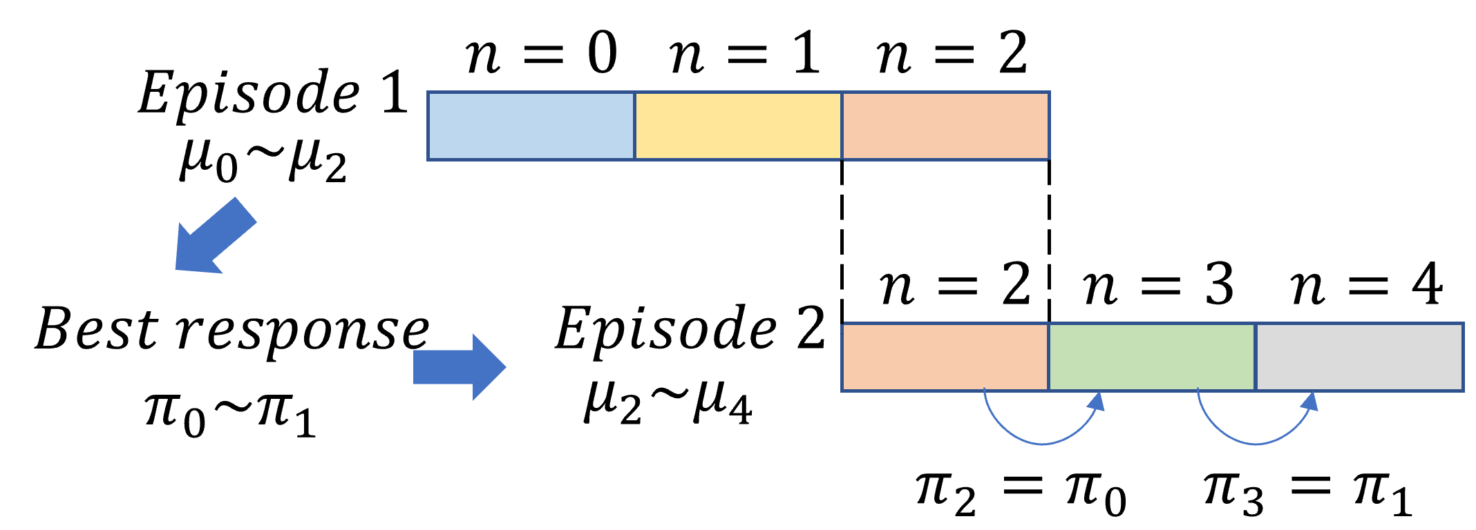
Figure 1: Illustration of the interaction process.

4.2 Definition

Formally, we first denote the mapping from an aggregate MF distribution sequence to the unique optimal policy sequence for type $i$ as $\Phi^{i}:\mathcal{M}\rightarrow\Pi^{i}$. For type $i$, we denote the mapping from a policy sequence to its induced MF distribution sequence starting from a specific initial distribution as $\Psi^{i}:\Pi^{i}\times\mathcal{P}(\mathcal{S}^{i})\rightarrow\mathcal{M}^{i}$.

Let us now formalize the interaction process using these notations. Given a joint MF distribution sequence (representing population behavior) ${\boldsymbol{\mu}}$, every sub-population $i$ solves the optimal policy sequence ${\boldsymbol{\pi}}^{i}=\Phi^{i}(\mathcal{B}{\boldsymbol{\mu}})$ and implements it starting from day $N-1$, inducing the next sequence ${\boldsymbol{\mu}}^{i+}=\Psi^{i}({\boldsymbol{\pi}}^{i},\mu^{i}_{N-1})$. The steady state of the system must satisfy ${\boldsymbol{\mu}}^{i}={\boldsymbol{\mu}}^{i+}$ for all types, which leads to the definition of the MUE as follows:

Definition 4.1

A pair $({\boldsymbol{\pi}},{\boldsymbol{\mu}})$ is called an MUE if for every type $i$

$${\boldsymbol{\pi}}^{i}=\Phi^{i}(\mathcal{B}{\boldsymbol{\mu}}),\quad{\boldsymbol{\mu}}^{i}=\Psi^{i}({\boldsymbol{\pi}}^{i},\mu^{i}_{N-1})$$

To facilitate discussion, denote the vector-valued functions

$$\Phi(\mathcal{B}{\boldsymbol{\mu}})=\begin{bmatrix}...\\ \Phi^{i}(\mathcal{B}{\boldsymbol{\mu}})\\ ...\end{bmatrix},\Psi({\boldsymbol{\pi}},{\boldsymbol{\mu}}_{N-1})=\begin{bmatrix}...\\ \Psi^{i}({\boldsymbol{\pi}}^{i},\mu_{N-1}^{i})\\ ...\end{bmatrix}$$

These two operators can be combined as $\Gamma({\boldsymbol{\mu}}):\prod_{i\in\mathcal{I}}\mathcal{M}^{i}\to\prod_{i\in\mathcal{I}}\mathcal{M}^{i}$, where $\Gamma({\boldsymbol{\mu}})=\Psi(\Phi(\mathcal{B}{\boldsymbol{\mu}}),{\boldsymbol{\mu}}_{N-1})$. Thus, the MUE is essentially a fixed point ${\boldsymbol{\mu}}=\Gamma({\boldsymbol{\mu}})$. In such states, commuters’ anticipation matches the actual population outcome, thus no one has the incentive to deviate from their current policy.

Note that as per the definition, the MUE $({\boldsymbol{\pi}},{\boldsymbol{\mu}})$ must have the same starting and ending joint distribution, that is ${\boldsymbol{\mu}}_{0}={\boldsymbol{\mu}}_{N-1}$. This condition arises because day $N-1$ is used twice in adjacent sequences within the interaction process. However, it is important to understand that the actual day $N-1$ only occurs once. The resulting cyclic behavior occurs from day $0$ to day $N-2$, with day $N-1$ essentially repeating day 0. To illustrate this in the context of Section 4.1, suppose the MUE is $\left\{\mu_{0},\mu_{1},\mu_{2}\right\}$. In the steady state, the system should follow a pattern of $\mu_{0},\mu_{1},\mu_{0},\mu_{1},\mu_{0},\mu_{1},...$, with the cycle repeating every two days rather than three.

Remark 4.2

It is also worth stressing the difference between the proposed MUE and conventional mean-field equilibrium or MFE. For the given initial distribution ${\boldsymbol{\mu}}_{0}\in\prod_{i\in\mathcal{I}}\mathcal{P}(\mathcal{S}^{i})$, an MFE $({\boldsymbol{\pi}},{\boldsymbol{\mu}})$ should satisfies ${\boldsymbol{\pi}}=\Phi({\boldsymbol{\mu}}),{\boldsymbol{\mu}}=\Psi({\boldsymbol{\pi}},{\boldsymbol{\mu}}_{0})$. Unlike the conventional MFE, the definition of MUE does not rely on any exogenous variable like ${\boldsymbol{\mu}}_{0}$. Further details on MFE can be found in Appendix 11.

Before studying the existence of the MUE, we first introduce a mild assumption. For every type $i$, the cost function $f^{i}(s,\nu)$ is continuous with respect to any $\nu\in\mathcal{P}(\mathcal{S})$ for all $s\in\mathcal{S}^{i}$.

With this assumption, we can establish the existence of the MUE by the following proposition. In this paper, otherwise specified, all proofs are provided in Appendix 12.

Proposition 4.3

Under Assumption 4.2, there always exists at least one MUE $({\boldsymbol{\pi}},{\boldsymbol{\mu}})$.

As Assumption 4.2 is generally satisfied in various travel choice scenarios, the existence of MUE makes such an equilibrium notion more appealing for transportation network analysis, as it provides a benchmark against which various improving transportation policies can be compared.

4.3 Connection with Wardrop Equilibrium

This section explores the relationship between a general MUE and the conventional Wardrop equilibrium or WE. In this paper, we refer WE as a general concept including the classic UE (Wardrop 1952) and other variants, where no commuter can reduce their actual or perceived cost by unilaterally switching their choices.

4.3.1 No inertia

As discussed earlier, user inertia influences and establishes connections between travel choices across adjacent days. The reason for planning ahead is to strike a balance between avoiding congestion and adjustments. When there is no inertia, commuters do not need to be foresighted. In this case, the MUE simplifies to the logit-based stochastic user equilibrium (logit-SUE), as demonstrated by the following proposition:

Proposition 4.4

When $d^{i}(s,s^{\prime})=0$ for all $i\in\mathcal{I}$ and $s,s^{\prime}\in\mathcal{S}^{i}$, the MUE repeats the logit-SUE every day.

4.3.2 Short planning horizon

Even in the presence of user inertia, when the planning horizon is very short (i.e. $N$=2), commuters essentially plan only for the next day. In this case, commuters are not being foresighted, reducing MUE to the state-dependent stochastic user equilibrium (SDSUE), a special equilibrium concept proposed in Castaldi, Delle Site, and Filippi (2017, 2019). To elaborate, we first present a definition of the SDSUE using our notations.

Definition 4.5

For type $i$, suppose the perceived disutility of choosing $a$ while the current choice is $s$ is $U_{s}^{a,i}=V_{s}^{a,i}+\delta$, where $s,a\in\mathcal{S}^{i}$. The deterministic cost $V_{s}^{a,i}$ satisfies $V_{s}^{a,i}=V^{a,i}+\epsilon\cdot\textbf{1}_{s\neq a}$, where $V^{a,i}$ is the disutility that only depends on $a$, while $\epsilon\cdot\textbf{1}_{s\neq a}$ is the switching cost between the two states. $\delta$ is an identical and independently distributed random term. Consider a choice model (e.g. logit model) $P_{s}^{a,i}=P_{s}^{a,i}(V_{s}^{a,i},a\in\mathcal{S}^{i})$. Let $q_{s}^{i}$ denote the proportion of type $i$ choosing state, then $\left\{q_{s}^{i}\right\}_{s\in\mathcal{S}^{i},i\in\mathcal{I}}$ is defined as a SDSUE if $q_{s}^{i}=\sum_{a\in\mathcal{S}^{i}}q_{a}^{i}P_{a}^{s,i}$ for all $a,s\in\mathcal{S}^{i}$ and $i\in\mathcal{I}$.

Remark 4.6

The original definition of SDSUE (Castaldi, Delle Site, and Filippi 2017, 2019) specifies the adjustment cost as $\epsilon\cdot\textbf{1}_{s\neq a}$ with the same $\epsilon$ for all commuters. Nonetheless, it can be easily generalized to another formulation of inertia. To maintain consistency, we will use the same formulation when discussing the connection with SDSUE.

The existence of SDSUE is generally ensured (Castaldi, Delle Site, and Filippi 2017, 2019). As can be seen from the definition, SDSUE is a similar concept to SUE but considers the inertia between travel choices. If the switching cost $\epsilon$ always equals 0, the SDSUE collapses back to conventional SUE. Following this line, the next proposition illustrates how the proposed MUE reduces to SDSUE when $N=2$.

Proposition 4.7

Using the travel cost and switching cost $f^{i}(a,\nu)+\epsilon\cdot\textbf{1}_{s\neq a}$ as $V_{s}^{a,i}$, the deterministic cost of changing from $s$ to $a$, the corresponding SDSUE is denoted as $\mu_{SDSUE}$. When $N=2$, the MUE repeats $\mu_{SDSUE}$ over the two days.

4.3.3 Stationary multiday user equilibrium

Before exploring further properties of the MUE, we introduce a new concept, stationary MUE (s-MUE), which is built upon the idea of stationary solutions presented in Gomes, Mohr, and Souza (2010). As illustrated in Figure 4.3.3, the s-MUE can be viewed as a special multiday equilibrium pattern where the MF distribution and policy remain invariant across consecutive days, regardless of the horizon length. In the figure, different colors represent different distribution patterns. Different from the MUE defined for finite horizon Markov games, the definition of s-MUE does not rely on exogenous horizon length. In this sense, it is similar to WE. However, as discussed later in this section, s-MUE is different from WE.

Illutration of the relationship between three types of equilibria

Formally, the s-MUE is defined as follows:

Definition 4.8

A pair $(\bar{V}^{1},...,\bar{V}^{I},\bar{\mu}^{1},...,\bar{\mu}^{I})$ or $(\boldsymbol{\bar{V}},{\boldsymbol{\bar{\mu}}})$, where $\bar{\mu}^{i}\in\mathcal{P}(\mathcal{S}^{i})$ and $\bar{V}^{i}\in\mathbb{R}^{M_{i}}/\mathbb{R}$, is called a s-MUE if it satisfies the following conditions for all type $i$:

• There exists a set of constants $\bar{\lambda}^{i}$ such that $\mathcal{G}_{\bar{\nu}}^{i}\bar{V}^{i}(s)=\bar{V}^{i}(s)+\bar{\lambda}^{i}$ for all $s\in\mathcal{S}^{i}$, where $\bar{\nu}=\mathcal{B}{\boldsymbol{\bar{\mu}}}$

• $\mathcal{K}_{\bar{\pi}^{i}}^{i}\bar{\mu}^{i}(s)=\bar{\mu}^{i}(s)$ for all $s\in\mathcal{S}^{i}$, where $\bar{\pi}^{i}$ is the unique optimal policy determined by $\bar{V}^{i}$ and $\bar{\nu}$.

The first condition implies that the policy is time-invariant since the relative value of the value function for different states remains the same. The second condition ensures the stationarity of the MF distribution.

To provide more insights into the s-MUE, consider that we enforce each state $s$ to have a final value $\bar{V}^{i}(s)$ for every type $i$. In this case, the pair $({\boldsymbol{\pi}},{\boldsymbol{\mu}})$ such that $\pi_{n}^{i}=\bar{\pi}^{i}$, $\mu_{n}^{i}=\bar{\mu}^{i}$ for all $n,i$ is an MUE. To see why, the first condition in the definition ensures the optimality of the policy, while the second condition ensures that the policy sequence can induce the MF distribution sequence. In this sense, an s-MUE is a special MUE with boundary conditions that require the final values to match with $\boldsymbol{\bar{V}}$. However, this requirement typically cannot be satisfied when commuters are making finite-horizon sequential decisions, where the final value should always be zero.

The following proposition establishes the existence of the s-MUE by assuming the boundness of costs. It is built on Theorem 3 in Gomes, Mohr, and Souza (2010), where we extend the original results to the multi-type case.

There exists $C>0$ such that for all $i\in\mathcal{I}$, $s,s^{\prime}\in\mathcal{S}^{i}$, and $\nu\in\mathcal{P}(\mathcal{S})$

$$0\leq f^{i}(s,\nu)\leq C,\quad 0\leq d^{i}(s,s^{\prime})\leq C$$

Proposition 4.9

When Assumption 4.2 and 4.3.3 hold, there always exists a s-MUE.

It is intriguing to ask what the s-MUE actually represents and how it is related to conventional WE. In fact, it can be seen as a ”generalized” version of SDSUE, specifically designed for foresighted commuters. The following proposition discusses it in more detail.

Proposition 4.10

Consider an s-MUE pair $(\boldsymbol{\bar{V}},{\boldsymbol{\bar{\mu}}})$. When using $\bar{V}^{i}(s^{\prime})+\epsilon\cdot\textbf{1}_{s\neq s^{\prime}}$ as the deterministic disutility of changing from $s$ to $s^{\prime}$ for type $i$, ${\boldsymbol{\bar{\mu}}}$ is the corresponding SDSUE.

Compared to the case with limited planning horizon (i.e. $N=2$) in Proposition 4.7, the only difference is that here we use the value function $\bar{V}^{i}$ instead of the travel cost $f^{i}(s,\nu)$. That reflects the difference between foresighted and myopic commuters: if we consider $f^{i}(s,\nu)$ as a daily disutility of state $s$, $\bar{V}^{i}(s)$ reflects the accumulated effects of disutility in the future. For instance, consider if $f^{i}(s,\bar{\nu})>f^{i}(s^{\prime},\bar{\nu})$, indicating state $s^{\prime}$ is more preferable in terms of daily travel cost, the superiority of state $s^{\prime}$, $\bar{V}^{i}(s^{\prime})$, should be more dominant for foresighted commuters. As they can plan for the future, choosing $s$ not only incurs more immediate travel costs but also leads to a higher likelihood of switching to other states, incurring more switching costs in the future.

5 Specific Choice Scenarios

So far, we have developed and analyzed a general Markov game model without specifying the choice scenario. In this section, we apply the general model to the choice of route and departure time respectively to derive more corresponding properties and connect them with existing literature, whenever possible.

5.1 Route Choices

In this section, we consider an infinite number of commuters making their route choices on a graph $(\mathcal{V},\mathcal{L})$, where $\mathcal{V},\mathcal{L}$ are the set of all the nodes and links respectively. Each OD pair corresponds to two nodes in $\mathcal{V}$, which are connected by several paths. Each path is comprised of links in $\mathcal{L}$. In the route choice scenario, each type may differ from each other in its OD pairs or value of time. $\mathcal{S}$ refers to the total set of available paths for all OD pairs, while the path set for type $i$ is denoted as $\mathcal{S}^{i}\subseteq\mathcal{S}$. For simplicity of analysis, assume that every link is covered by some paths.

For a fixed total demand $\xi$, the path flow of type $i$ on path $s$ on day $n$ is simply $\xi\mu^{i}_{n}(s)$. In addition, the flow on link $l\in\mathcal{L}$ can be expressed as $x(l,\nu_{n}):\mathcal{L}\times\mathcal{P}(\mathcal{S})\rightarrow\mathbb{R}$, where $x(l,\nu_{n})=\sum_{s\in\mathcal{S}}\xi\nu_{n}(s)\delta_{l,s}$. $\delta_{l,s}$ equals $1$ if link $l$ is on route $s$, and $0$ otherwise. By introducing the link-path incidence matrix $\Delta=[\delta_{l,s}]_{l\in\mathcal{L},s\in\mathcal{S}}\in\mathbb{R}^{|\mathcal{L}|\times|\mathcal{S}|}$, we can write the link flow vector using a bold notation ${\boldsymbol{x}}(\nu_{n})=\xi\Delta\nu_{n}=\xi\Delta\mathcal{B}{\boldsymbol{\mu}}_{n}$, where $\mathcal{B}$ is again the linear operator from joint to aggregate distribution as in Section 3.

In route choices, we consider that the travel cost solely stems from the travel time. Thus, the travel cost for type $i$ is $f^{i}(s,\nu)=\kappa_{i}f(s,\nu)$, where $f(s,\nu)$ is the travel time of path $s$, and $\kappa_{i}$ is the value of time for type $i$. Let $t_{l}\left(x(l,\nu)\right)$ denote the link travel time on $l$, then the path travel time is $f(s,\nu)=\sum_{l\in\mathcal{L}}t_{l}\left(x(l,\nu)\right)\delta_{l,s}$. In this section, the link travel time $t_{l}(x)$ is chosen as the so-called BPR function (Bureau of Public Roads 1964) $t_{l}(x)=t_{l}^{0}\left[1+\beta_{l}\left(\frac{x}{c_{l}}\right)^{4}\right]$, where $t_{l}^{0}$ is the free flow travel time; $c_{l}$ is the capacity and $\beta_{l}$ is a parameter.

In our discussion, we will primarily employ $d^{i}(s,s^{\prime})=\epsilon^{i}\cdot\mathbf{1}_{s\neq s^{\prime}}$ to model the switching cost for route choices as in Delle Site (2018), where $\epsilon^{i}$ is the inertia weight for type $i$. This suggests a uniform penalty for switching to any different route. Other distance functions can also be used. For example, it could be inversely related to the route overlap between $s$ and $s^{\prime}$, implying that changing to a more familiar route would result in a lower inertia cost.

We first update the continuity assumption, which is more tailored for the route choice model. [Modified version of Assumption 4.2] The link cost function $t_{l}(x)$ is continuous for every link $l\in\mathcal{L}$.

Assumption 5.1 can lead to Assumption 4.2, which further ensures the existence of the MUE, as presented in the following corollary. We skip the proof as it is trivial.

Corollary 5.1

Under Assumption 5.1, there always exists at least one MUE $({\boldsymbol{\pi}},{\boldsymbol{\mu}})$.

We introduce another assumption that establishes the monotonicity of the link travel time. It is mild and can be satisfied by a range of models including the BPR function.

The link travel time $t_{l}(v)$ is strictly monotone and increasing for all link $l\in\mathcal{L}$.

With these assumptions in place, we explore several key properties related to route choices. We will begin by discussing the uniqueness of the flow pattern in the MUE.

5.1.1 Unique flow

Although the MUE may not be unique, we can demonstrate that every MUE should have distinct starting and ending path flows, which is detailed in the following proposition

Proposition 5.2

Under the Assumption 5.1 and 5.1, if two MUEs have the same initial path flow, they must have the same path flow evolution over the planning horizon.

Meanwhile, we also demonstrate that every s-MUE must have a unique link flow using the following proposition.

Proposition 5.3

When Assumption 4.3.3, 5.1, 5.1 hold, if $(\boldsymbol{\bar{V}},{\boldsymbol{\bar{\mu}}})$ and $(\boldsymbol{\bar{V}}^{\prime},{\boldsymbol{\bar{\mu}}}^{\prime})$ are both s-MUE, they must have the same link flow pattern.

5.1.2 Between-day variations

As we discussed in Section 4.3.3, s-MUE maintains time-invariant MF distribution but requires certain boundary conditions on final values, which typically do not hold when commuters are making finite-horizon sequential decisions. As illustrated in the following proposition, this discrepancy will lead to the fact that MUE always has between-day variations on the MF distribution sequence.

Proposition 5.4

In non-trivial cases (i.e. $N>2$, $\epsilon^{i}>0$ for all $i$, and uniform path choices cannot generate equal path costs for all ODs), every MUE cannot have a time-invariant path flow.

To bring more insights into the last case, consider the parallel routing on three identical links. If commuters choose evenly among the three paths, the resulting path costs are equal. In such cases, the MUE can maintain invariant path flow. However, these cases are very rare.

While prior research has explored how user inertia affects network equilibrium flow patterns, as documented in Lou, Yin, and Lawphongpanich (2010), Di et al. (2013) and Zhang and Yang (2015), our study uncovers novel phenomena. We demonstrate that user inertia can lead to variations in traffic flow patterns from day to day, even in steady-state conditions. This occurs as commuters engage in strategic, sequential decision-making across a planning horizon.

5.1.3 Asymptotic pattern

The MUE flow can appear somewhat chaotic due to between-day variations. However, the MUE demonstrates certain patterns when the planning horizon tends toward infinity. Specifically, the s-MUE begins to emerge within the MUE, either at the center or at the two ends. This asymptotic behavior is detailed in the following proposition, providing valuable insights into the long-term flow pattern of transportation networks.

Proposition 5.5

Without losing generality, assume the episode length is even, and denote the episode as $\mathcal{N}=\left\{0,1,...,2k-1\right\}$. When the episode length is $2k$, denote the corresponding MUE as $({\boldsymbol{\pi}}^{(2k)},{\boldsymbol{\mu}}^{(2k)})$. Under Assumption 5.1 and 5.1 , for every $\delta>0$, there exists $K$ such that for all $k\geq K$, either the link flow on day 0 or day $k$ of $({\boldsymbol{\pi}}^{(2k)},{\boldsymbol{\mu}}^{(2k)})$ is $\delta$-close to the link flow of s-MUE.

5.2 Departure Time Choices

In this section, we examine departure time choices, considering a discrete version of the classic Vickrey bottleneck model for the morning commute problem (Vickrey 1969). Typically, the departure time window and the arrival time are assumed to be homogeneous for all commuters, although they may vary in their cost preferences. Therefore, $\mathcal{S}=\mathcal{S}^{i}$ for all $i$, where the state space $\mathcal{S}$ refers to the allowable departure time window, and each state $s$ is a time slice within the window. The length of the departure time window is denoted as $L$ hours, with each time slice being $\frac{L}{M}$ hours.

In this context, $\mu^{i}_{n}(s)$ refers to the proportion of commuters within type $i$ departing at $s$ on day $n$, and $\nu_{n}(s)$ is equivalent to the departure rate of the entire population at time $s$. Consequently, denote the total number of commuters is $\xi$, then the number of commuters that depart at time $s$ on day $n$ is $\xi\nu_{n}(s)$.

Without losing generality, we ignore the free-flow travel time, and thus travel time experienced by commuters only consists of the queuing delay at the bottleneck. The discrete version of the travel time function proposed by Han, Friesz, and Yao (2013) is adopted:

$$T(s,\nu_{n})=\sum_{x\in\mathcal{S},x\leq s}\frac{\nu_{n}(x)}{C_{b}}-s-\min_{y\in\mathcal{S},y\leq s}\left\{\sum_{x\in\mathcal{S},x\leq y}\frac{\nu_{n}(x)}{C_{b}}-y\right\}$$

where $T(s,\nu_{n})$ refers to the travel time in day $n$; $C_{b}$ refers to the ”normalized” bottleneck capacity, which is $C_{b}=\frac{C_{b}^{*}}{\xi}\frac{L}{M}$, where $C_{b}^{*}$ is the true capacity in the unit of commuters per hour, and $y$ refers to the nearest time that the inflow is below the capacity.

Suppose the desired arrival time for type $i$ is $r^{i}$, then the travel cost function is given by:

$$f^{i}(s,\nu_{n}):=\alpha^{i}T(s,\nu_{n})+\beta^{i}[r^{i}-s-T(s,\nu_{n})]_{+}+\gamma^{i}[s+T(s,\nu_{n})-r^{i}]_{+}$$

where $\alpha^{i},\beta^{i},\gamma^{i}$ are the penalty coefficients for travel time, early arrival and late arrival for type $i$, and $[r-s-T(s,\mu_{n})]_{+}=\max\left\{r-s-T(s,\mu_{n}),0\right\}$. We consider the adjustment cost to be a distance function, $d^{i}(s,s^{\prime})=\epsilon^{i}\cdot|s-s^{\prime}|$.

We can affirm that the travel cost considering scheduling cost is always continuous, which ensures the existence of MUE for departure time choices. However, due to the complex structure of the cost function, it remains an open question whether the MUE is unique, or how the MUE behaves asymptotically.

Corollary 5.6

$T(s,\nu_{n})$ is a continuous function and thus there will always exist at least one MUE.

6 Numerical Examples

In this section, we introduce an algorithm to compute the approximate MUE and two numerical examples of route and departure time choice problems to illustrate the proposed model.

6.1 Solution Algorithm

Inspired by the Fictitious Play (FP) algorithm (Perrin et al. 2020, Elie et al. 2020), we propose Adaptive Initial Distribution - Fictitious Play (AID-FP), as presented in Algorithm 1. In AID-FP, to smoothen commuters’ interaction process and enhance convergence, we compute the average of all previous optimal responses rather than using only the most recent one. Then, we calculate the MF distribution sequence induced by the average policy starting from the final distribution of the previous round by recursively using Equation (3). The induced sequence is further used to calculate the new optimal response in the next iteration by recursively using Equation (1) and (2). One behavioral interpretation of the algorithm is that, during the interaction process, only a proportion of the population updates their policy to the best response at the beginning of each episode, while the others are content with and maintain their current policy. Note that in Algorithm 1, we always use the joint distribution and policy of all types, and the superscript $j$ now refers to the iteration index rather than types. Compared to conventional FP used to solve MFE, AID-FP does not require a predetermined initial distribution for each iteration, which is a better fit for our model.

We define the following two measurements of convergence for the output of each iteration:

• Exploitability (Perrin et al. 2020, Perolat et al. 2022): This metric measures how far the output policy is from the best response. For a pair $({\boldsymbol{\pi}},{\boldsymbol{\mu}})$, the exploitability of type $i$ is defined as $\phi^{i}({\boldsymbol{\pi}},{\boldsymbol{\mu}})=J^{i}_{\mathcal{B}{\boldsymbol{\mu}}}({\boldsymbol{\pi}})-\min_{{\boldsymbol{\pi}}^{\prime}\in\Pi^{i}}J^{i}_{\mathcal{B}{\boldsymbol{\mu}}}({\boldsymbol{\pi}}^{\prime})$. The overall exploitability of the entire population is $\phi({\boldsymbol{\pi}},{\boldsymbol{\mu}})=\sum_{i\in\mathcal{I}}\phi^{i}({\boldsymbol{\pi}},{\boldsymbol{\mu}})$.

• Difference at the two ends: This metric measures the distance between the starting and ending joint distribution, i.e. $D({\boldsymbol{\mu}})=d_{J}({\boldsymbol{\mu}}_{0},{\boldsymbol{\mu}}_{N-1})$, where $d_{J}$ is the metric defined for the joint distribution in Appendix 10.

If both measurements converge to zero, the output is guaranteed to be an MUE. Now we use the algorithm as a heuristic to solve the model and leave the theoretical proof of convergence for future work.

Algorithm 1 AID-FP

Input: An initial joint distribution over all types ${\boldsymbol{\mu}}_{0}$; An initial joint policy sequence ${\boldsymbol{\pi}}^{0}$; Calculate the MF distribution sequence ${\boldsymbol{\bar{\mu}}}^{0}$ induced by ${\boldsymbol{\pi}}^{0}$ starting from ${\boldsymbol{\mu}}_{0}$
      Output: $({\boldsymbol{\bar{\pi}}}^{J},{\boldsymbol{\bar{\mu}}}^{J})$

1:for $j=1,2,\ldots,J$ do

2:     Compute ${\boldsymbol{\pi}}^{j}$, the optimal response policy against the aggregate sequence $\mathcal{B}{\boldsymbol{\bar{\mu}}}^{j-1}$

3:     Update the average policy ${\boldsymbol{\bar{\pi}}}^{j}=\frac{j-1}{j}{\boldsymbol{\bar{\pi}}}^{j-1}+\frac{1}{j}{\boldsymbol{\pi}}^{j}$,

4:     Compute ${\boldsymbol{\bar{\mu}}}^{j}$, the MF distribution sequence induced by ${\boldsymbol{\bar{\pi}}}^{j}$ starting from ${\boldsymbol{\bar{\mu}}}^{j-1}_{N-1}$

5:end for

6.2 Route Choices

In this section, the proposed model is applied to the Nguyen-Dupuis network (Nguyen and Dupuis 1984) as shown in Figure 6.2. There are four OD pairs in total, i.e., OD 1 (Node 1$\rightarrow$ Node 2), OD 2 (Node 1$\rightarrow$ Node 3), OD 3 (Node 4$\rightarrow$ Node 2), and OD 4 (Node 4$\rightarrow$ Node 3). The OD demands consist of 4,130 vehicles per hour for OD 1 and OD 4, and 1,870 vehicles per hour for the other two OD pairs. In total, the network comprises 19 links and 25 paths, as specified in Table 1. The link performance function is $t(x)=3\left[1+4\left(\frac{x}{2200}\right)^{4}\right]$ minutes for all links. We consider the planning horizon of $N=7$ days. For convenience, we assume that all commuters within each OD pair are homogeneous, categorizing them into four types. The value of time is set to 1 and the dispersion parameter $\theta$ equals 1 for all demands. Moreover, the inertia cost takes the form of $d^{i}(s,s^{\prime})=\epsilon^{i}\cdot\textbf{1}_{s=s^{\prime}}$, and each OD pair may differ from each other in terms of the inertia weight $\epsilon^{i}$.

Nguyen and Dupuis Network

OD pair	Path No.	Link No.
1-2	1	3,4,5,10,16
	2	3,4,8,10,14
	3	3,7,8,10,13
	4	6,7,8,10,11
	5	1,4,5,12,16
	6	1,4,8,12,14
	7	1,7,8,12,13
	8	1,16,19
1-3	9	3,4,10,14,15
	10	3,7,10,13,15
	11	6,7,10,11,15
	12	9,10,11,18
	13	1,4,12,14,15
	14	1,7,12,13,15
4-2	15	2,3,4,5,16
	16	2,3,4,8,14
	17	2,3,7,8,13
	18	2,6,7,8,11
	19	6,7,8,17
4-3	20	2,3,4,14,15
	21	2,3,7,13,15
	22	2,6,7,11,15
	23	2,9,11,18
	24	6,7,15,17
	25	9,17,18

Table 1: Path-link relationship

6.2.1 No inertia

We begin by examining a special case without user inertia. Here, we set all the inertia weights $\epsilon^{1}$ to $\epsilon^{4}$ to 0.

Figure 6.2.1 illustrates the convergence of the algorithm in this scenario. The blue dotted curve represents the exploitability, while the green curve shows the difference between the starting and ending distributions. Both curves consistently converge to zero, demonstrating the successful convergence of the algorithm. Consequently, the final output is confirmed to be an MUE.

Convergence of the algorithm in the case without user inertia

To provide an overview of the resulting MUE, Figure 6.2.1 displays the MUE path flow over all 7 days. The dots on each curve represent the path flow on that day. Here we use curves connecting dots on the same day to better demonstrate the evolution. Notably, the curves on different days perfectly overlap, indicating that all path flows remain time-invariant over the 7 days. For a more detailed depiction of the flow pattern, Figure 6.2.1 showcases path flows for the first three routes from OD 1. In this representation, each curve illustrates the flow evolution of a single path over the planning horizon, and it clearly shows that the path flows remain unchanged across all days.

MUE without user inertia

Path flow on route 1,2,3

Furthermore, the travel cost on the last day $f(s,\nu_{N-1})$ as well as the augmeneted cost $f(s,\nu_{N-1})+\frac{1}{\theta^{i}}\ln(\xi\mu_{N-1}^{i}(s))$ are plotted together in Figure 6.2.1. Each path incurs different travel costs, as indicated by the blue bars. However, paths within the same OD pair share a nearly identical augmented cost, depicted by the green bars. Given the invariance of path flows over the planning horizon, this observation suggests that the resulting MUE consistently reproduces the logit-SUE flow every day, which agrees with the analysis in Section 4.3.

Travel cost of each path

6.2.2 With inertia

In a general case with user inertia, we set $\epsilon^{1}=3$ and $\epsilon^{2},\epsilon^{3},\epsilon^{4}=1$, indicating that commuters in OD 1 exhibit greater sensitivity to adjustments. Figure 6.2.2 demonstrates a similar convergence pattern to the previous case, indicating that the algorithm successfully converges to an MUE.

Convergence of the algorithm in the case with user inertia

Figure 6.2.2 provides an overview of the resulting MUE. As before, each sub-figure plots 7 curves, which represent the path flow over the 7 days. Unlike the previous scenario, where path flows remained constant over the planning horizon, this time there are between-day variations. These fluctuations are evident as the path flow curves do not overlap. To examine these variations more closely, Figure 6.2.2 offers a detailed view of the flows on path 1 and path 3. The blue and green solid curves show the path flow evolution for these two paths, indicating the existence of fluctuations. Moreover, the path flows exhibit a cyclic pattern, starting and ending at the same flow level, which is in line with the requirements of an MUE. Figure 6.2.2 also includes the path flow for the s-MUE, represented by the green and blue dotted lines, as these values remain constant. The MUE flow on path 1 starts a higher level than the s-MUE but later falls below it. Conversely, the flow on path 3 is consistently remain below the s-MUE path flow.

MUE of the route choices with user inertia

Path flow on route 1 and 3

6.3 Departure Time Choices

In this section, we apply the bottleneck model setting in Guo et al. (2018). The total number of commuters is $6,000$, and the capacity of the bottleneck is $c=3,000$ vehicles per hour. In line with typical bottleneck model assumptions, we consider all commuters to be homogeneous. The penalty for travel time, early arrival and late arrival are $\alpha=10,\beta=5,\gamma=15$, respectively. The departure time window on each day is $[0,3]$ hours, which is further discretized into $M=40$ slices. Thus, the length of each slice (i.e. each state) is $0.075$ hours or 4.5 minutes. The desired arrival time for all commuters is $r=2$ and the planning horizon also contains $N=7$ days. Here we use $d(s,s^{\prime})=\epsilon\cdot|s-s^{\prime}|$ as the switching cost, where not only the frequency but also the adjustment range matter. We set the inertia weight $\epsilon$ and the dispersion parameter $\theta$ to $1$ and $0.5$, respectively.

In Figure 6.3, we illustrate the convergence of the algorithm. Similar to the route choice cases, both measurements converge effectively to 0, indicating the successful computation of the MUE.

Convergence of the algorithm in departure time choices

Figure 6.3 presents the resulting MUE, which features seven curves representing the departure rate profile for each day throughout the planning horizon. Zooming in on the curves around the peak reveals an interesting pattern. The population begins with the blue curve on the first day and continues to fluctuate around the red line from day 2 to day 6, eventually returning to the blue curve on day 7. Moreover, the MUE exhibits a distinct pattern compared to the user equilibrium, represented by the green dotted line. While both cases feature two peaks, the departure time profile of the MUE is more concentrated in the middle of the range. This concentration results from the presence of inertia and perception error, which lead commuters to prefer staying in the middle of the departure time window to avoid substantial adjustments.

MUE of departure time choices

To provide a more detailed view of the departure rate pattern, we focus on the rate evolution at 1.2 hours over the planning horizon in Figure 6.3. Each node in the graph corresponds to the departure rate on that specific day. The graph shows that the departure rate starts and ends at the same position, which is consistent with the definition of MUE. Furthermore, the figure demonstrates that between-day variations also exist for departure time choices. Moreover, Figure 6.3 also incorporates the s-MUE departure rate at time 1.2 hours, indicated by the dotted line. Notably, the MUE departure rate consistently remains below the s-MUE, but the values stay closely at the midpoint of the horizon.

Departure rate evolution over the planning horizon

7 Model Extensions

In this section, we will concisely explore potential extensions to enhance the scope of the proposed model. Although these extensions might add complexity, they can be integrated within the current framework without fundamental changes.

7.1 More General Heterogeneity

In the proposed model, the multi-type population influences each other through aggregate population behavior. This approach effectively reduces the dimension of the interaction process and is particularly suitable for routing scenarios. However, it may fail to account for more general and complex forms of heterogeneity. For instance, when analyzing departure time choices with the bathtub model, it is crucial to consider heterogeneity in factors such as trip distances, as noted by Fosgerau (2015), Jin (2020). Regrettably, the model encounters difficulties in representing this heterogeneity through the use of an aggregate distribution.

To address this limitation, we could employ the joint distribution in place of the aggregate one. This adjustment allows for tracking the departure profile of each sub-population that shares the same trip length. This modified framework resembles the one proposed by Perolat et al. (2022), where the cost function of state $s$ becomes $f(s,{\boldsymbol{\mu}})$ rather than $f(s,\nu)$. Although this enhancement enriches the model’s versatility while maintaining its core framework, a formal definition and thorough analysis of the extension are outside the scope of this paper.

7.2 Different Planning Length

The proposed model assumes a uniform planning horizon of $N$ for all commuters. Yet, in practice, commuters may have diverse planning horizons for various reasons. For example, automated vehicle companies may implement different algorithms in their vehicles, resulting in commuters with different levels of foresight.

Consider a scenario with two sub-populations, whose planning horizon is 4 and 7 days respectively. The interaction between these sub-populations is illustrated in Figure 7.2. At the end of day 3, the first sub-population updates its policy based on the aggregate behavior in the first 4 days, prompting the next sequence $\mu_{3}^{1}\sim\mu_{6}^{1}$. Then, on the close of day 6, this sub-population updates its policy again, leading to $\mu_{6}^{1}\sim\mu_{9}^{1}$, while the second population also updates its policy, resulting in $\mu_{6}^{2}\sim\mu_{12}^{2}$. This pattern allows us to consider every 7-day cycle. If the joint population behavior over the 7-day span (containing one update of sub-population 1) remains invariant throughout the interaction process, it can be considered the MUE of the system. Although a formal definition and analysis of this extended MUE are not included in this text, this modification demonstrates the model’s flexibility in accommodating different planning horizons. It paves the way for further investigation into how various sub-populations with distinct planning durations interact and achieve equilibrium in complex transportation networks.

Illustration of the system with multiple planning lengths

8 Conclusion and Future Work

In this research, we have developed a comprehensive model that captures the multiday traffic patterns arising from commuters’ sequential decision-making on their travel choices. To achieve this, we first framed individual decision-making as an optimal control problem. Given the interdependence of multiple commuters in the system, we introduced the concept of multiday user equilibrium to represent the steady state of their interaction. At this equilibrium, each commuter behaves optimally, and no one can reduce their overall cost through unilateral adjustments to their policy sequences. General properties were analyzed without focusing on any specific travel choice. The results were further used to derive corresponding properties for route and departure time choices. Two numerical experiments were conducted to illustrate the proposed model. In addition, we also briefly discussed how to extend the model to accommodate more general cost structures and different lengths of planning horizon.

Broadly speaking, our study offers a general framework for modeling individual sequential decision-making and the corresponding system equilibrium. While our primary focus in this paper has been on trip choices under user inertia, the model’s flexibility allows for generalization to other scenarios where individual behavior is associated with some Markov decision process. Additionally, our research reveals the fingerprint left by user inertia on steady states. Even when demand and supply remain constant, the presence of user inertia, particularly among foresighted commuters, leads to between-day traffic flow variations in steady states. Moreover, our work also establishes crucial connections between the multiday user equilibrium and the conventional Wardrop equilibrium in three scenarios: no inertia, short and infinitely-long planning horizon.

For future studies, we anticipate exploring scenarios with imperfect and incomplete information, since each player may only know partial information about the population. It is also interesting to investigate the learning process before reaching equilibrium, where agents update their policies while observing the information based on their daily experiences. Another interesting direction to theoretically extend the current work is to incorporate myopic agents who make one-shot decisions.

The work described in this paper was partly supported by research grants from National Science Foundation (CMMI-1904575 and CMMI-2233057) and the USDOT University Transportation Center for Connected and Automated Transportation (CCAT).

9 Notation Table

Table 2: Notations

Sets
$n\in\mathcal{N}$		Planning horizon, with $N=|\mathcal{N}|$
$\mathcal{S}$		Overall state space, with $M=|\mathcal{S}|$
$i\in\mathcal{I}$		Set of commuter types, with $I=|\mathcal{I}|$
$\mathcal{S}^{i}$		State space for type $i$, with $M^{i}=|\mathcal{S}^{i}|$
$l\in\mathcal{L}$		Set of links
Variables
$s_{n}^{i}\in\mathcal{S}^{i}$		State of type $i$ on day $n$
$a_{n}^{i}\in\mathcal{S}^{i}$		Action of type $i$ on day $n$
$\mu_{n}^{i}\in\mathcal{P}(\mathcal{S}^{i})$		MF distribution of type $i$ on day $n$
${\boldsymbol{\mu}}_{n}\in\prod_{i\in\mathcal{I}}\mathcal{P}(\mathcal{S}^{i})$		Joint distribution of all types on day $n$
${\boldsymbol{\mu}}^{i}\in\mathcal{M}^{i}$		MF distribution sequence of type $i$
${\boldsymbol{\mu}}\in\prod_{i\in\mathcal{I}}\mathcal{M}^{i}$		Joint MF distribution sequence
$\pi_{n}^{i}$		Policy of type $i$ on day $n$
${\boldsymbol{\pi}}^{i}\in\Pi^{i}$		Policy sequence of type $i$
${\boldsymbol{\pi}}\in\prod_{i\in\mathcal{I}}\Pi^{i}$		Joint policy sequence
$\nu_{n}\in\mathcal{P}(\mathcal{S})$		Aggregate MF distribution on day $n$
${\boldsymbol{\nu}}\in\mathcal{M}$		Aggregate MF distribution sequence
Paramters
$\rho_{i}$		Proportion of type $i$
$\omega_{i}$		Contribution weight of type $i$
$\theta^{i}$		Dispersion parameter of type $i$
$\epsilon^{i}$		Inertia weight of type $i$
$C$		Upper bound of cost functions
$\xi$		Total demand
$\kappa_{i}$		Value of time for type $i$
$L$		Length of the departure time window
$C_{b}$		Normalized bottleneck capacity
$\alpha^{i},\beta^{i},\gamma^{i}$		Penalty for early arrival, travel time and late arrival
Functions
$\mathcal{B}$		Aggregation operator
$c^{i}(s,s^{\prime},\nu_{n},\pi_{n,s})$		The total cost of type $i$ on day $n$
$f^{i}(s,\nu_{n})$		The travel cost of type $i$ on day $n$
$d^{i}(s,s^{\prime})$		The switching cost of type $i$
$J_{{\boldsymbol{\nu}}}^{i}({\boldsymbol{\pi}}^{i})$		The total cost of type $i$
$V_{n}^{i,{\boldsymbol{\nu}},{\boldsymbol{\pi}}^{i}}$, $V_{n}^{i,{\boldsymbol{\nu}}}$		The policy and optimal value function for type $i$ on day $n$
$\mathcal{G}_{\boldsymbol{\nu}}^{i,\pi}$, $\mathcal{G}_{{\boldsymbol{\nu}}}^{i}$		The policy and optimal Bellman operator for type $i$
$\mathcal{K}^{i}_{\pi}$		Flow conservation operator for type $i$
$\Phi^{i}$		Optimal response mapping for type $i$
$\Psi^{i}$		Flow conservation mapping for type $i$
$\Gamma$		Overall multiday user equilibrium operator
${\boldsymbol{x}}(\nu)$		The link flow vector
$t_{l}(x)$		Travel time on link $l$

10 Metrics

The the metrics of $\mathcal{M}^{i}$ ($\mathcal{M}$), $\prod_{i\in\mathcal{I}}\mathcal{P}(\mathcal{S}^{i})$, $\prod_{i\in\mathcal{I}}\mathcal{M}^{i}$, $\Pi^{i}$ ($\Pi$) and $\prod_{i\in\mathcal{I}}\Pi^{i}$ are defined as follows

$$d_{M}({\boldsymbol{\mu}}^{i},{\boldsymbol{\tilde{\mu}}}^{i})=\max_{n\in\mathcal{N}}d_{f}(\mu^{i}_{n},\tilde{\mu}^{i}_{n})\quad{\boldsymbol{\mu}}^{i},{\boldsymbol{\tilde{\mu}}}^{i}\in\mathcal{M}^{i}$$

$$d_{J}({\boldsymbol{\mu}}_{n},{\boldsymbol{\tilde{\mu}}}_{n})=\max_{i\in\mathcal{I}}d_{f}(\mu^{i}_{n},\tilde{\mu}^{i}_{n})\quad{\boldsymbol{\mu}}^{i},{\boldsymbol{\tilde{\mu}}}^{i}\in\prod_{i\in\mathcal{I}}\mathcal{P}(\mathcal{S}^{i})$$

$$d_{MS}({\boldsymbol{\mu}},{\boldsymbol{\tilde{\mu}}})=\max_{i\in\mathcal{I}}\max_{n\in\mathcal{N}}d_{f}(\mu^{i}_{n},\tilde{\mu}^{i}_{n})\quad{\boldsymbol{\mu}},{\boldsymbol{\tilde{\mu}}}\in\prod_{i\in\mathcal{I}}\mathcal{M}^{i}$$

$$d_{P}({\boldsymbol{\pi}}^{i},{\boldsymbol{\tilde{\pi}}}^{i})=\max_{n\in\mathcal{N}}\max_{s\in\mathcal{S}^{i}}d_{f}(\pi^{i}_{n}(\cdot|s),\tilde{\pi}_{n}^{i}(\cdot|s))\quad{\boldsymbol{\pi}}^{i},{\boldsymbol{\tilde{\pi}}}^{i}\in\Pi^{i}$$

$$d_{PS}({\boldsymbol{\pi}},{\boldsymbol{\tilde{\pi}}})=\max_{i\in\mathcal{I}}\max_{n\in\mathcal{N}}\max_{s\in\mathcal{S}^{i}}d_{f}(\pi^{i}_{n}(\cdot|s),\tilde{\pi}_{n}^{i}(\cdot|s))\quad{\boldsymbol{\pi}},{\boldsymbol{\tilde{\pi}}}\in\prod_{i\in\mathcal{I}}\Pi^{i}$$

Proposition 10.1

The metric spaces $(\mathcal{M}^{i},d_{M}),(\mathcal{M},d_{M}),(\prod_{i\in\mathcal{I}}\mathcal{P}(\mathcal{S}^{i}),d_{J})$, $(\prod_{i\in\mathcal{I}}\mathcal{M}^{i},d_{MS})$, $(\Pi^{i},d_{P})$, $(\Pi,d_{P})$ and $(\prod_{i\in\mathcal{I}}\Pi^{i},d_{PS})$ are complete metric spaces for all types.

Proof 10.2

Proof of Proposition 10.1: Consider the metric space $(\mathcal{M}^{i},d_{M})$. With minor abuse of notation, let $\left\{{\boldsymbol{\mu}}^{i(j)}\right\}_{j\in\mathbb{N}}$ be a Cauchy sequence, where ${\boldsymbol{\mu}}^{i(j)}\in\mathcal{M}^{i}$. Note that here the superscript $j$ is the index for the Cauchy sequence and $i$ is for the type. For any $\sigma>0$, there exists $K\in\mathbb{N}$ such that for all $k,l>K$, we have

$$d_{M}({\boldsymbol{\mu}}^{i(k)},{\boldsymbol{\mu}}^{i(l)})=\max_{n\in\mathcal{N}}d_{f}(\mu^{i(k)}_{n},\mu^{i(l)}_{n})<\sigma$$

It indicates

$$d_{f}(\mu^{i(k)}_{n},\mu^{i(l)}_{n})=\max_{s\in\mathcal{S}^{i}}|\mu_{n}^{i(k)}(s)-\mu_{n}^{i(l)}(s)|<\sigma\qquad\forall n\in\mathcal{N}$$

Hence

$$|\mu_{n}^{i(k)}(s)-\mu_{n}^{i(l)}(s)|<\sigma\qquad\forall n\in\mathcal{N},s\in\mathcal{S}^{i}$$

As $\mathbb{R}$ is complete, for all $n\in\mathcal{N},s\in\mathcal{S}^{i}$, $\left\{\mu_{n}^{i(j)}(s)\right\}_{j\in\mathbb{N}}$ has a limit, which is denoted by $\mu^{i}_{n}(s)$. Denoting ${\boldsymbol{\mu}}^{i}=\left\{\mu^{i}_{n}\right\}_{n\in\mathcal{N}}$, we have ${\boldsymbol{\mu}}^{i(j)}\rightarrow{\boldsymbol{\mu}}^{i}$, and the limit is also in $\mathcal{M}^{i}$. It indicates the completeness of $\mathcal{M}^{i}$. Similarly, we can prove the completeness of other spaces.

11 Mean-field equilibrium

The multiday user equilibrium (MUE) is closely related to the concept of mean-field equilibrium (MFE), which is widely discussed in the literature. To better demonstrate their relationship and facilitate the proof later, we first give a brief discussion on MFE. To keep aligned with the proposed model, we restate the definition of MFE using the aggregate distribution

Definition 11.1

For a given ${\boldsymbol{\mu}}_{0}\in\prod_{i\in\mathcal{I}}\mathcal{P}(\mathcal{S}^{i})$, a pair $({\boldsymbol{\pi}},{\boldsymbol{\mu}})$ is called an MFE if the following holds for every type $i$

$${\boldsymbol{\pi}}^{i}=\Phi^{i}(\mathcal{B}{\boldsymbol{\mu}}),\quad{\boldsymbol{\mu}}^{i}=\Psi^{i}({\boldsymbol{\pi}}^{i},\mu^{i}_{0})$$

where $\Phi^{i},\Psi^{i}$ are the same as Section 4. For simplicity, we also denote it shortly as

$${\boldsymbol{\pi}}=\Phi(\mathcal{B}{\boldsymbol{\mu}}),\quad{\boldsymbol{\mu}}=\Psi({\boldsymbol{\pi}},{\boldsymbol{\mu}}_{0})$$

As can be seen, different from MUE, the definition of MFE typically requires an exogenous ${\boldsymbol{\mu}}_{0}$ as the fixed initial distribution. In this sense, MUE can be viewed as a special MFE, which is further illustrated in the following proposition. We omit the proof as it is trivial.

Proposition 11.2

On the one hand, every MFE with the same initial and final distribution is an MUE. On the other hand, every MUE is an MFE with a special initial distribution.

12 Proofs of the main results

12.1 Results in Section 4

12.1.1 Proof of Proposition 4.3:

We first introduce a lemma.

Lemma 12.1

For any type $i$, any policy sequences ${\boldsymbol{\pi}},{\boldsymbol{\tilde{\pi}}}\in\Pi^{i}$ such that $d_{P}({\boldsymbol{\pi}},{\boldsymbol{\tilde{\pi}}})\leq\epsilon$, and any two MF distribution $\mu_{0},\tilde{\mu}_{0}\in\mathcal{P}(\mathcal{S}^{i})$ such that $d_{f}(\mu_{0},\tilde{\mu}_{0})\leq\epsilon$, denote ${\boldsymbol{\mu}}=\Psi^{i}({\boldsymbol{\pi}},\mu_{0})$ and ${\boldsymbol{\tilde{\mu}}}=\Psi^{i}({\boldsymbol{\tilde{\pi}}},\tilde{\mu}_{0})$. We have

$$d_{M}({\boldsymbol{\mu}},{\boldsymbol{\tilde{\mu}}})\leq\frac{M^{N}-1}{M-1}\epsilon$$

Proof 12.2

Proof: We first prove that $d_{f}(\mu_{n},\tilde{\mu}_{n})\leq\frac{M^{n+1}-1}{M-1}\epsilon$ by induction. It clearly holds at $n=0$. Now suppose it holds at $n=k$ for $k\geq 0$. For $n=k+1$, we have

$$\begin{split}|\mu_{k+1}(s)-\tilde{\mu}_{k+1}(s)|&=\left|\sum_{s^{\prime}\in\mathcal{S}^{i}}\mu_{k}(s^{\prime})\pi_{k}(s|s^{\prime})-\sum_{s^{\prime}\in\mathcal{S}^{i}}\tilde{\mu}_{k}(s^{\prime})\tilde{\pi}_{k}(s|s^{\prime})\right|\\ &\leq\sum_{s^{\prime}\in\mathcal{S}^{i}}\pi_{k}(s|s^{\prime})|\mu_{k}(s^{\prime})-\tilde{\mu}_{k}(s^{\prime})|+\sum_{s^{\prime}\in\mathcal{S}^{i}}\tilde{\mu}_{k}(s^{\prime})|\pi_{k}(s|s^{\prime})-\tilde{\pi}_{k}(s|s^{\prime})|\\ &\leq Md_{f}(\mu_{k},\tilde{\mu}_{k})+\epsilon\\ &\leq\frac{M^{k+2}-1}{M-1}\epsilon\end{split}$$

where the first inequality can be proved by adding and subtracting $\sum_{s^{\prime}\in\mathcal{S}}\tilde{\mu}_{k}(s^{\prime})\pi_{k}(s|s^{\prime})$ within the absolute value, and the second inequality is from $d_{P}({\boldsymbol{\pi}}^{i},{\boldsymbol{\tilde{\pi}}})\leq\epsilon$. As the bound holds for all $s\in\mathcal{S}^{i}$, we prove by induction that $d_{f}(\mu_{n},\tilde{\mu}_{n})\leq\frac{M^{n+1}-1}{M-1}\epsilon$ holds for all $n\in\mathcal{N}$. Then, we can use the largest $n=N-1$ to bound $d_{M}({\boldsymbol{\mu}},{\boldsymbol{\tilde{\mu}}})$, which proves the lemma. $\blacksquare$

Now we are ready to prove the theorem. We identify each $\mathcal{M}^{i}$ with simplex $\mathcal{X}_{|\mathcal{N}|(|\mathcal{S}^{i}|-1)}\subseteq\mathbb{R}^{|\mathcal{N}|(|\mathcal{S}^{i}|-1)}$ and $\Pi^{i}$ with simplex $\mathcal{X}_{|\mathcal{N}||\mathcal{S}^{i}|(|\mathcal{S}^{i}|-1)}\subseteq\mathbb{R}^{|\mathcal{N}||\mathcal{S}^{i}|(|\mathcal{S}^{i}|-1)}$. Since $\prod_{i\in\mathcal{I}}\mathcal{M}^{i}$ is the cartesian product of simplices, we also identify $\prod_{i\in\mathcal{I}}\mathcal{M}^{i}$ as a subset of some Euclidean spaces. Recall the mapping $\Gamma({\boldsymbol{\mu}}):\prod_{i\in\mathcal{I}}\mathcal{M}^{i}\to\prod_{i\in\mathcal{I}}\mathcal{M}^{i}$, where $\Gamma({\boldsymbol{\mu}})=\Psi(\Phi(\mathcal{B}{\boldsymbol{\mu}}),{\boldsymbol{\mu}}_{N-1})$. We now check the requirements for Brouwer’s fixed-point theorem.

The finite-dimensional simplices are convex, closed, and bounded, hence compact. Since $\prod_{i\in\mathcal{I}}\mathcal{M}^{i}$ is the cartesian product of simplices, it is also convex and compact.

The value function $\left\{V_{n}^{i}\right\}_{i\in\mathcal{I},n\in\mathcal{N}}$ is recursively calculated by

$$V^{i}_{n}(s)=f^{i}(s,\nu_{n})-\frac{1}{\theta^{i}}\ln\left[\sum_{a\in\mathcal{S}^{i}}e^{-\theta^{i}(d^{i}(s,a)+V_{n+1}^{i}(a))}\right]$$

with the terminal condition $V^{i}_{N}(s)=0$ for all $s\in\mathcal{S}^{i}$. Since the finite sum, product, and composition of continuous functions is also continuous, we can obtain the continuity of the map ${\boldsymbol{\nu}}\to V_{n}^{i}(s)$ for all $n\in\mathcal{N},i\in\mathcal{I},s\in\mathcal{S}^{i}$. Since $\mathcal{B}$ is a linear operator, it also ensures the continuity of ${\boldsymbol{\mu}}\to{\boldsymbol{\nu}}$, therefore the mapping ${\boldsymbol{\mu}}$ to $V^{i}_{n}(s)$ is continuous for all $n,i,s$. Further, the optimal policy is calculated by

$$\pi^{i}_{n}(s^{\prime}|s)=\frac{e^{-\theta^{i}(d^{i}(s,s^{\prime})+V^{i}_{n+1}(s^{\prime}))}}{\sum_{a\in\mathcal{S}^{i}}e^{-\theta^{i}(d^{i}(s,a)+V^{i}_{n+1}(a))}}$$

Since $\sum_{a\in\mathcal{S}^{i}}e^{-\theta^{i}(d^{i}(s,a)+V^{i}_{n+1}(a))}\neq 0$ always holds, we can similarly obtain the continuity of $\left\{V_{n}^{i}\right\}_{n\in\mathcal{N}}\to\pi_{n}^{i}$ for all $n,i$, which further proves the continuity of the mapping ${\boldsymbol{\mu}}\to\Phi^{i}(\mathcal{B}{\boldsymbol{\mu}})$.

Now consider the mapping for type $i$, $\Gamma^{i}({\boldsymbol{\mu}})=\Psi^{i}(\Phi^{i}(\mathcal{B}{\boldsymbol{\mu}}),\mu_{N-1}^{i})$. For any $\epsilon>0$ and for any ${\boldsymbol{\tilde{\mu}}}\in\prod_{i\in\mathcal{I}}\mathcal{M}^{i}$, denote $\Phi^{i}(\mathcal{B}{\boldsymbol{\tilde{\mu}}})$ as ${\boldsymbol{\tilde{\pi}}}^{i}$. Due to the continuity of ${\boldsymbol{\mu}}\to\Phi^{i}(\mathcal{B}{\boldsymbol{\mu}})$, there exists $\delta_{1}$ such that for all ${\boldsymbol{\mu}}$ where $d_{M}({\boldsymbol{\mu}},{\boldsymbol{\tilde{\mu}}})\leq\delta_{1}$, there must be $d_{P}(\Phi^{i}(\mathcal{B}{\boldsymbol{\mu}}),{\boldsymbol{\tilde{\pi}}}^{i})\leq\epsilon$. Denote $\Phi^{i}(\mathcal{B}{\boldsymbol{\mu}})$ as ${\boldsymbol{\pi}}^{i}$.

Take $\delta_{2}=\min\left\{\epsilon,\delta_{1}\right\}$, then for all ${\boldsymbol{\mu}}\in\prod_{i\in\mathcal{I}}\mathcal{M}^{i}$ such that $d_{M}({\boldsymbol{\mu}},{\boldsymbol{\tilde{\mu}}})\leq\delta_{2}$, we have $d_{P}({\boldsymbol{\pi}}^{i},{\boldsymbol{\tilde{\pi}}})\leq\epsilon$ and $d_{f}(\mu_{N-1}^{i},\tilde{\mu}^{i}_{N-1})\leq\epsilon$. For any type $i$, we have $d_{M}(\Gamma^{i}({\boldsymbol{\mu}}),\Gamma^{i}({\boldsymbol{\tilde{\mu}}}))\leq\frac{M^{N}-1}{M-1}\epsilon$ based on Lemma 12.1. As the coefficient is finite, we prove the continuity of $\Gamma^{i}$. Further, since every item in $\Gamma({\boldsymbol{\mu}})$ is continuous, we obtain the continuity of $\Gamma({\boldsymbol{\mu}})$.

Thus, by Brouwer’s fixed-point theorem, there exists a fixed point ${\boldsymbol{\mu}}^{*}$ such that ${\boldsymbol{\mu}}^{*}=\Gamma({\boldsymbol{\mu}}^{*})$, which yields an MUE $(\Phi(\mathcal{B}{\boldsymbol{\mu}}^{*}),{\boldsymbol{\mu}}^{*})$.

12.1.2 Proof of Proposition 4.4:

Denote the MUE as $({\boldsymbol{\pi}},{\boldsymbol{\mu}})$, and denote ${\boldsymbol{\nu}}=\mathcal{B}{\boldsymbol{\mu}}$. The proposition is equivalent to that for any $n\in\mathcal{N}$ and $i\in\mathcal{I}$, $f^{i}(s,\nu_{n})+\frac{1}{\theta^{i}}\ln\mu^{i}_{n}(s)$ is equal for all state $s\in\mathcal{S}^{i}$.

For any type $i$, denote the optimal value function as $\left\{V^{i}_{n}\right\}_{n\in\mathcal{N}}$, then the unique optimal policy on day $n$ is $\pi^{i}_{n}(s^{\prime}|s)=\frac{e^{-\theta^{i}V^{i}_{n+1}(s^{\prime})}}{\sum_{z\in\mathcal{S}^{i}}e^{-\theta^{i}V^{i}_{n+1}(z)}}$. As can be seen, the policy has nothing to do with the previous state $s\in\mathcal{S}^{i}$, thus $\pi_{n}^{i}(s^{\prime}|s)$ is the same for all $s$. As a result, with flow conservation, we have $\mu_{n+1}^{i}(s^{\prime})=\pi_{n}^{i}(s^{\prime}|s)$. Further, taking log on both sides of Equation (1) yields the following equation for all $n\geq 1$:

$$V^{i}_{n}(s)+\frac{1}{\theta^{i}}\ln\mu^{i}_{n}(s)=-\frac{1}{\theta^{i}}\ln\sum_{s^{\prime}\in\mathcal{S}^{i}}e^{-\theta^{i}V^{i}_{n}(s^{\prime})}$$ (4)

We now prove the proposition by induction. For every type $i$, we know $V^{i}_{N}(s)=0$ for all $s\in\mathcal{S}^{i}$. By Equation (2), $V_{N-1}^{i}(s)=f^{i}(s,\nu_{N-1})-\frac{1}{\theta^{i}}\ln M^{i}$. Therefore

$$f^{i}(s,\nu_{N-1})+\frac{1}{\theta^{i}}\ln\mu^{i}_{N-1}(s)=\frac{1}{\theta^{i}}\left(\ln M^{i}-\ln\sum_{s^{\prime}\in\mathcal{S}^{i}}e^{-\theta^{i}V^{i}_{N-1}(s^{\prime})}\right)$$

where the right-hand side is the same for all $s\in\mathcal{S}^{i}$.

Now, suppose there exists $K\geq 1$ such that for all $n>K$, $f^{i}(s,\nu_{n})+\frac{1}{\theta^{i}}\ln\mu^{i}_{n}(s)$ is the same value for all $i\in\mathcal{I}$ and $s\in\mathcal{S}^{i}$. We know that $\pi_{K}^{i}(s^{\prime}|s)=\mu^{i}_{K+1}(s^{\prime})$ for all $s,s^{\prime}\in\mathcal{S}^{i}$, thus

$$V^{i}_{K}(s) =\sum_{s^{\prime}\in\mathcal{S}^{i}}\pi^{i}_{K}(s^{\prime}|s)\left(f^{i}(s,\nu_{K})+\frac{1}{\theta^{i}}\ln\pi^{i}_{K}(s^{\prime}|s)+V^{i}_{K+1}(s^{\prime})\right)$$

$$=\sum_{s^{\prime}\in\mathcal{S}^{i}}\mu^{i}_{K+1}(s^{\prime})\left(f^{i}(s,\nu_{K})-\frac{1}{\theta^{i}}\ln\sum_{s^{\prime}\in\mathcal{S}^{i}}e^{-\theta^{i}V^{i}_{K+1}(s^{\prime})}\right)=f^{i}(s,\nu_{K})-\frac{1}{\theta^{i}}\ln\sum_{s^{\prime}\in\mathcal{S}^{i}}e^{-\theta^{i}V^{i}_{K+1}(s^{\prime})}$$

Substituting it into Equation (4) yields

$$f^{i}(s,\nu_{K})+\frac{1}{\theta^{i}}\ln\mu^{i}_{K}(s)=\frac{1}{\theta^{i}}\left(\ln\sum_{s^{\prime}\in\mathcal{S}^{i}}e^{-\theta^{i}V^{i}_{K+1}(s^{\prime})}-\ln\sum_{s^{\prime}\in\mathcal{S}^{i}}e^{-\theta^{i}V^{i}_{K}(s^{\prime})}\right)$$

where the right-hand side is also the same for all $s\in\mathcal{S}^{i}$. By induction, we know that the proposition holds for all $n\geq 1$. Note that the starting distribution is the same as the ending distribution, therefore the proposition also holds for $n=0$.

12.1.3 Proof of Proposition 4.7

Since the MUE shares the same starting and ending distribution, we denote it as ${\boldsymbol{\mu}}={\boldsymbol{\mu}}_{0}={\boldsymbol{\mu}}_{1}$. Denote $\nu=\mathcal{B}{\boldsymbol{\mu}}$. For any type $i$, since $V_{2}^{i}(s)=0$ holds for all $s\in\mathcal{S}^{i}$, Equation (2) yields

$$V_{1}^{i}(s)=f^{i}(s,\nu)-\frac{1}{\theta^{i}}\ln\left((M^{i}-1)e^{-\theta^{i}\epsilon}+1\right)$$

Thus, the optimal policy on day 0 is

$$\pi_{0}^{i}(s^{\prime}|s)=\frac{e^{-\theta^{i}(\epsilon\cdot\textbf{1}_{s\neq s^{\prime}}+f^{i}(s^{\prime},\nu))}}{\sum_{z\in\mathcal{S}}e^{-\theta^{i}(\epsilon\cdot\textbf{1}_{s\neq z}+f^{i}(z,\nu))}}$$

which is essentially the logit model $P_{s}^{s^{\prime},i}$ given the disutility. Since ${\boldsymbol{\mu}}_{0}={\boldsymbol{\mu}}_{1}={\boldsymbol{\mu}}$, ${\boldsymbol{\pi}}_{0}$ can maintain ${\boldsymbol{\mu}}$ invariant, hence $\mu^{i}(s^{\prime})=\sum_{s\in\mathcal{S}^{i}}P_{s}^{s^{\prime},i}\mu^{i}(s)$ naturally holds for all types. Consequently, $\left\{\mu^{i}(s)\right\}_{i\in\mathcal{I},s\in\mathcal{S}^{i}}$ is an SDSUE.

12.1.4 Proof of Proposition 4.9

We first introduce the following lemma, which extends Proposition 5 in Gomes, Mohr, and Souza (2010) to multitype cases.

Lemma 12.3

For any type $i$, $\nu\in\mathcal{P}(\mathcal{S})$ and $V\in\mathbb{R}^{M_{i}}$, the following equation holds for all $s,s^{\prime}\in\mathcal{S}^{i}$

$$|\mathcal{G}_{\nu}^{i}V(s)-\mathcal{G}_{\nu}^{i}V(s^{\prime})|\leq 2C$$

References

- Ameli et al. (2022) Ameli M, Faradonbeh MSS, Lebacque JP, Abouee-Mehrizi H, Leclercq L, 2022 Departure time choice models in urban transportation systems based on mean field games. Transportation Science 56(6):1483–1504.
- Aurell and Djehiche (2019) Aurell A, Djehiche B, 2019 Modeling tagged pedestrian motion: A mean-field type game approach. Transportation research part B: methodological 121:168–183.
- Beckmann, McGuire, and Winsten (1956) Beckmann M, McGuire CB, Winsten CB, 1956 Studies in the economics of transportation. Technical report.
- Bensoussan, Huang, and Lauriere (2018) Bensoussan A, Huang T, Lauriere M, 2018 Mean field control and mean field game models with several populations. arXiv preprint arXiv:1810.00783 .
- Boyles, Tang, and Unnikrishnan (2015) Boyles SD, Tang S, Unnikrishnan A, 2015 Parking search equilibrium on a network. Transportation Research Part B: Methodological 81:390–409.
- Bureau of Public Roads (1964) Bureau of Public Roads, 1964 Traffic Assignment Manual (U.S. Dept. of Commerce, Urban Planning Division).
- Cabannes et al. (2021) Cabannes T, Lauriere M, Perolat J, Marinier R, Girgin S, Perrin S, Pietquin O, Bayen AM, Goubault E, Elie R, 2021 Solving n-player dynamic routing games with congestion: a mean field approach. arXiv preprint arXiv:2110.11943 .
- Castaldi, Delle Site, and Filippi (2017) Castaldi C, Delle Site P, Filippi F, 2017 Stochastic user equilibrium in the presence of inertia. Transportation Research Procedia 22:13–24.
- Castaldi, Delle Site, and Filippi (2019) Castaldi C, Delle Site P, Filippi F, 2019 Stochastic user equilibrium in the presence of state dependence. EURO Journal on Transportation and Logistics 8(5):535–559.
- Chen, He, and Yin (2016) Chen Z, He F, Yin Y, 2016 Optimal deployment of charging lanes for electric vehicles in transportation networks. Transportation Research Part B: Methodological 91:344–365.
- Cirant (2015) Cirant M, 2015 Multi-population mean field games systems with neumann boundary conditions. Journal de Mathématiques Pures et Appliquées 103(5):1294–1315.
- Cui and Koeppl (2021) Cui K, Koeppl H, 2021 Approximately solving mean field games via entropy-regularized deep reinforcement learning. International Conference on Artificial Intelligence and Statistics, 1909–1917 (PMLR).
- Daganzo and Sheffi (1977) Daganzo CF, Sheffi Y, 1977 On stochastic models of traffic assignment. Transportation science 11(3):253–274.
- Delle Site (2018) Delle Site P, 2018 A mixed-behaviour equilibrium model under predictive and static advanced traveller information systems (atis) and state-dependent route choice. Transportation Research Part C: Emerging Technologies 86:549–562.
- Di et al. (2013) Di X, Liu HX, Pang JS, Ban XJ, 2013 Boundedly rational user equilibria (brue): mathematical formulation and solution sets. Procedia-Social and Behavioral Sciences 80:231–248.
- Elie et al. (2020) Elie R, Perolat J, Laurière M, Geist M, Pietquin O, 2020 On the convergence of model free learning in mean field games. Proceedings of the AAAI Conference on Artificial Intelligence, volume 34, 7143–7150.
- Feleqi (2013) Feleqi E, 2013 The derivation of ergodic mean field game equations for several populations of players. Dynamic Games and Applications 3:523–536.
- Fosgerau (2015) Fosgerau M, 2015 Congestion in the bathtub. Economics of Transportation 4(4):241–255.
- Fudenberg et al. (1998) Fudenberg D, Drew F, Levine DK, Levine DK, 1998 The theory of learning in games, volume 2 (MIT press).
- Gomes, Mohr, and Souza (2010) Gomes DA, Mohr J, Souza RR, 2010 Discrete time, finite state space mean field games. Journal de mathématiques pures et appliquées 93(3):308–328.
- Guo et al. (2018) Guo RY, Yang H, Huang HJ, Li X, 2018 Day-to-day departure time choice under bounded rationality in the bottleneck model. Transportation Research Part B: Methodological 117:832–849.
- Han, Friesz, and Yao (2013) Han K, Friesz TL, Yao T, 2013 A partial differential equation formulation of vickrey’s bottleneck model, part i: Methodology and theoretical analysis. Transportation Research Part B: Methodological 49:55–74.
- Huang et al. (2021) Huang K, Chen X, Di X, Du Q, 2021 Dynamic driving and routing games for autonomous vehicles on networks: A mean field game approach. Transportation Research Part C: Emerging Technologies 128:103189.
- Huang, Malhamé, and Caines (2006) Huang M, Malhamé RP, Caines PE, 2006 Large population stochastic dynamic games: closed-loop mckean-vlasov systems and the nash certainty equivalence principle. Communications in Information & Systems 6(3):221–252.
- Iryo (2019) Iryo T, 2019 Instability of departure time choice problem: A case with replicator dynamics. Transportation Research Part B: Methodological 126:353–364.
- Jin (2020) Jin WL, 2020 Generalized bathtub model of network trip flows. Transportation Research Part B: Methodological 136:138–157.
- Lasry and Lions (2007) Lasry JM, Lions PL, 2007 Mean field games. Japanese journal of mathematics 2(1):229–260.
- Lin, Yin, and He (2021) Lin X, Yin Y, He F, 2021 Credit-based mobility management considering travelers’ budgeting behaviors under uncertainty. Transportation Science 55(2):297–314.
- Liu et al. (2017) Liu W, Li X, Zhang F, Yang H, 2017 Interactive travel choices and traffic forecast in a doubly dynamical system with user inertia and information provision. Transportation Research Part C: Emerging Technologies 85:711–731.
- Lou, Yin, and Lawphongpanich (2010) Lou Y, Yin Y, Lawphongpanich S, 2010 Robust congestion pricing under boundedly rational user equilibrium. Transportation Research Part B: Methodological 44(1):15–28.
- Mahmassani and Chang (1987) Mahmassani HS, Chang GL, 1987 On boundedly rational user equilibrium in transportation systems. Transportation science 21(2):89–99.
- Nguyen and Dupuis (1984) Nguyen S, Dupuis C, 1984 An efficient method for computing traffic equilibria in networks with asymmetric transportation costs. Transportation Science 18(2):185–202.
- Perolat et al. (2022) Perolat J, Perrin S, Elie R, Laurière M, Piliouras G, Geist M, Tuyls K, Pietquin O, 2022 Scaling Mean Field Games by Online Mirror Descent. Proceedings of the International Joint Conference on Autonomous Agents and Multiagent Systems, AAMAS, volume 2, 1028–1037, ISBN 9781713854333, URL www.ifaamas.org.
- Perrin et al. (2020) Perrin S, Pérolat J, Laurière M, Geist M, Elie R, Pietquin O, 2020 Fictitious play for mean field games: Continuous time analysis and applications. Advances in Neural Information Processing Systems 33:13199–13213.
- Qi et al. (2023) Qi H, Jia N, Qu X, He Z, 2023 Investigating day-to-day route choices based on multi-scenario laboratory experiments, part i: Route-dependent attraction and its modeling. Transportation Research Part A: Policy and Practice 167:103553.
- Shou et al. (2022) Shou Z, Chen X, Fu Y, Di X, 2022 Multi-agent reinforcement learning for markov routing games: A new modeling paradigm for dynamic traffic assignment. Transportation Research Part C: Emerging Technologies 137:103560.
- Smith (1984) Smith MJ, 1984 The stability of a dynamic model of traffic assignment—an application of a method of lyapunov. Transportation science 18(3):245–252.
- Srinivasan and Mahmassani (2000) Srinivasan KK, Mahmassani HS, 2000 Modeling inertia and compliance mechanisms in route choice behavior under real-time information. Transportation Research Record 1725(1):45–53.
- Tajeddini and Kebriaei (2018) Tajeddini MA, Kebriaei H, 2018 A mean-field game method for decentralized charging coordination of a large population of plug-in electric vehicles. IEEE Systems Journal 13(1):854–863.
- Thorhauge, Swait, and Cherchi (2020) Thorhauge M, Swait J, Cherchi E, 2020 The habit-driven life: accounting for inertia in departure time choices for commuting trips. Transportation Research Part A: Policy and Practice 133:272–289.
- Urata et al. (2021) Urata J, Xu Z, Ke J, Yin Y, Wu G, Yang H, Ye J, 2021 Learning ride-sourcing drivers’ customer-searching behavior: A dynamic discrete choice approach. Transportation research part C: emerging technologies 130:103293.
- Vickrey (1969) Vickrey WS, 1969 Congestion Theory and Transport Investment. The American Economic Review 59(2):251–260, URL http://www.jstor.org/stable/1823678.
- Wardrop (1952) Wardrop JG, 1952 Road paper. some theoretical aspects of road traffic research. Proceedings of the institution of civil engineers 1(3):325–362.
- Xie et al. (2021) Xie Q, Yang Z, Wang Z, Minca A, 2021 Learning while playing in mean-field games: Convergence and optimality. International Conference on Machine Learning, 11436–11447 (PMLR).
- Zhang and Yang (2015) Zhang J, Yang H, 2015 Modeling route choice inertia in network equilibrium with heterogeneous prevailing choice sets. Transportation Research Part C: Emerging Technologies 57:42–54.
- Zhang et al. (2023) Zhang K, Mittal A, Djavadian S, Twumasi-Boakye R, Nie YM, 2023 Ride-hail vehicle routing (river) as a congestion game. Transportation Research Part B: Methodological 177:102819.