On global in time self-similar solutions of Smoluchowski equation with multiplicative kernel

Abstract

We study the similarity solutions (SS) of Smoluchowski coagulation equation with multiplicative kernel $K(x,y)=(xy)^{s}$ for $s<\frac{1}{2}$. When $s<0$, the SS consists of three regions with distinct asymptotic behaviours. The appropriate matching yields a global description of the solution consisting of a Gamma distribution tail, an intermediate region described by a lognormal distribution and a region of very fast decay of the solutions to zero near the origin. When $s\in\left(0,\frac{1}{2}\right)$, the SS is unbounded at the origin. It also presents three regions: a Gamma distribution tail, an intermediate region of power-like (or Pareto distribution) decay and the region close to the origin where a singularity occurs. Finally, full numerical simulations of Smoluchowski equation serve to verify our theoretical results and show the convergence of solutions to the selfsimilar regime.

1 Introduction

Coagulation processes lie at the heart of numerous physical phenomena such as planetesimal accumulation, mergers in dense clusters of stars, aerosol coalescence in atmospheric physics, colloids and polymerization and gelation (see [9], [11], [16], [17]). In these processes, the basic mechanism is the aggregation of two small particles to create larger particles. Such aggregation will take place with a given probability that depends on the size of the particles, and the basic issue to solve concerns the expected evolution of the particle size distribution with time. The first model for coagulation processes was introduced by Smoluchowski in 1916 (cf. [21]). If we denote the particle size distribution by $c(x,t)$ and the probabilty of aggretation of two particles of size $x$ and $y$ respectively by $K(x,y)$, Smoluchowski equation reads

$$c_{t}\left(x,t\right)=\frac{1}{2}\int_{0}^{x}K\left(x-y,y\right)c\left(x-y,t\right)c\left(y,t\right)dy-c\left(x,t\right)\int\limits_{0}^{\infty}K\left(x,y\right)c\left(y,t\right)dy.$$ (1)

where the first term at the right hand side represents the number of particles of size $x$ that are created per unit time from the merging of two particles of sizes $x$ and $x-y$ respectively, and the second term at the right hand side represents the number of particles of size $x$ that merge with particles of arbitrary size per unit time.

Despite its formal simplicity, the nonlinear and nonlocal character of equation (1) lead to formidable difficulties for the analysis of its solutions. Explicit solutions are only available for a limited number of kernels $K(x,y)$ (cf. [19] for a general review and [2], [3] for a broad and recent account of the current mathematical theory for coagulation-fragmentation models). Two of these particular cases are $K(x,y)=1$ and $K(x,y)=xy$. Both cases belong to the broader family of multiplicative kernels $K(x,y)=(xy)^{s}$, $s\in\mathbb{R}$. In the first case, $s=0$, solutions exist globally in time while, in the second, solutions are such that sufficiently high moments $\int x^{n}c(x,t)dx$ ($n$ large enough) may blow up in finite time giving rise to a phenomenon known as gelation (see for instance [15], [23], [13], [20]).

In this paper we consider Smoluchowski equation with a multiplicative kernel:

$$c_{t}(x,t)=\frac{1}{2}\int_{0}^{x}(x-y)^{s}y^{s}c(x-y)c(y)dy-x^{s}c(x)\int_{0}^{\infty}y^{s}c(y)dy,$$ (2)

in the case $s<\frac{1}{2}$. In this range of parameters, solutions with all their moments bounded are expected to exist for all time $t>0$ and behave asymptotically as $t\rightarrow\infty$ in a selfsimilar manner, that is

$$c(x,t)\sim t^{\alpha}f(t^{\beta}x),$$ (3)

in a sense to be precissed and for suitable exponents $\alpha$, $\beta$. The scaling of equation (2) leads automatically to the relation $\alpha=(2s+1)\beta-1$, but $\beta$ remains as a free parameter that needs to be determined as part of the solution. From the physical point of view, a result as (3) contains the essential information on the behaviour of the system under consideration and measurable quantities such as exponents and similarity profiles $f(\xi)$ that can be measured experimentally and lead to direct physical consequences. It is therefore essential to elucidate whether such solutions exist and, if so, what is their shape and essential properties. In a broader sense, equations analogous in structure to (2) appear in models of turbulence and results like (3) are the central issue in connection with the development and structure of turbulent cascades (see [7], [8] and references therein). Knowing the shape and essential properties of similarity solutions $f(\xi)$ is also relevant in practical applications where a coagulation process takes place and its evolution is measured experimentally. In these cases, one wants to know what is the kernel $K(x,y)$ and hence the essential physical processes involved.

In this paper we compute, by means of matched asymptotic expansions, the similarity solutions $f(\xi)$ together with the similarity exponent $\beta$ to equation (2) for $s<0$. For $s\in\left(0,\frac{1}{2}\right)$ we compute the similarity solutions and develop asymptotic expansions for $\beta$ as a function of $s$ with $s$ sufficiently small. Finally, full numerical simulation of (2) is carried out in order to further support our matched asymptotic expansions and to show convergence of the solution $c(x,t)$ of (2) towards the selfsimilar regime. Our results coincide with results obtained by Cañizo and Mischler [6] (see also [12]) in the range $s\in\left(-\frac{1}{2},\frac{1}{2}\right)$ concerning asymptotic behaviour of selfsimilar solutions at the origin and generalize them to other regions in the parameter space as well as provide further information on the asymptotics away from the origin. In particular, the case $s\in\left(0,\frac{1}{2}\right)$ requires a novel procedure (previously developed and justified with full mathematical rigour in the context of gelation in finite time in [5]) for the computation of $\beta$ and this translates into special asymptotics for the solution.

A summary of our results is provided in Figures 1 and 2. For $s<0$, $\beta(s)=-1/(1-2s)$ and the similarity solutions consist of three regions: I) a region of very fast decay to zero near the origin, II) an intermediate region where the solution approximates a Lognormal distribution function and III) a region extending to infinity where the solution approaches a Gamma distribution function. For $s>0$ and sufficiently small, $\beta(s)=-1-2s+O(s^{2})$ and the solutions also consist of three regions: I) a singularity developing at the origin, II) a power-like decay or Pareto distribution function, III) a Gamma distribution extending up to infinity.

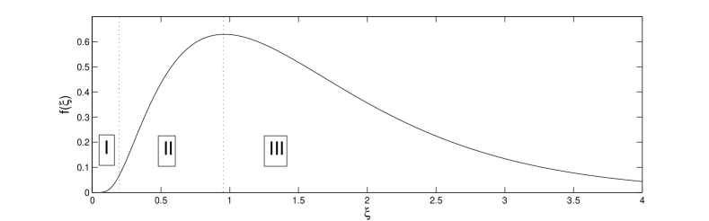
Figure 1: Structure of the selfsimilar solution for $s<0$. There exist three regions whose respective behaviours can be described as (I) very vast decay at the origin, (II) Lognormal distribution function, (III) Gamma distribution function.

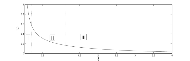
Figure 2: Structure of the selfsimilar solution for $s\in\left(0,\frac{1}{2}\right)$. There exist three regions whose respective behaviours can be described as (I) singularity at the origin, (II) Pareto distribution function, (III) Gamma distribution function.

2 The integrodifferential equation for selfsimilar solutions

By plugging the selfsimilar expression

$$c(x,t)=t^{\alpha}f(t^{\beta}x),$$

into (2), choosing

$$\alpha=\left(2s+1\right)\beta-1,$$

and defining

$$\xi:=t^{\beta}x,$$

we obtain the integrodifferential ordinary differential equation

$$\left(\left(2s+1\right)\beta-1\right)f(\xi)+\beta\xi f_{\xi}(\xi)=\frac{1}{2}\int_{0}^{\xi}(\xi-\eta)^{s}\eta^{s}f(\xi-\eta)f(\eta)d\eta-\xi^{s}f(\xi)\int_{0}^{\infty}\eta^{s}f(\eta)d\eta\ .$$ (4)

$\beta$ is a free parameter that has to be chosen, for a given $s$, from the condition that all the moments

$$M_{n}=\int_{0}^{\infty}x^{n}c(x,t)dx,\ n=1,2,\ldots,$$

remain bounded for $0<t<\infty$.

Notice that one can rearrange terms in the more convenient (for the purpose of analysis) form

$$\left(\left(2s+1\right)\beta-1\right)f(\xi)+\beta\xi f_{\xi}(\xi)$$ (5)

$$= \frac{1}{2}\int_{0}^{\xi}\eta^{s}\left[(\xi-\eta)^{s}f(\xi-\eta)f(\eta)-2\chi_{\frac{\xi}{2}}(\eta)\xi^{s}f(\xi)f(\eta)\right]d\eta$$

$$-\xi^{s}f(\xi)\int_{\frac{\xi}{2}}^{\infty}\eta^{s}f(\eta)d\eta,$$

where $\chi_{\frac{\xi}{2}}(\eta)$ is the characteristic function so that $\chi_{\frac{\xi}{2}}(\eta)=1$ for $\eta\leq\frac{\xi}{2}$ and zero elsewhere.

A different approach to the problem is through the use of Laplace transform:

$$C(\mu,t)=\int_{0}^{\infty}(e^{-\mu x}-1)c(x,t)dx.$$

By multiplying equation (2) $(e^{-\mu x}-1)$, integrating in $x$ and using

$$\int_{0}^{\infty}e^{-\mu x}\left(\int_{0}^{x}(x-y)^{s}y^{s}c(x-y,t)c(y,t)dydx\right)$$

$$= \int_{0}^{\infty}\int_{0}^{x}e^{-\mu y}e^{-\mu(x-y)}(x-y)^{s}y^{s}c(x-y,t)c(y,t)dydx$$

$$= \left(\int_{0}^{\infty}e^{-\mu y}y^{s}c(y,t)dy\right)^{2},$$

we arrive at the equation

$$C_{t}(\mu,t)=\frac{1}{2}\left(D_{\mu}^{-s}C(\mu,t)\right)^{2},$$

where

$$D_{\mu}^{-s}C(\mu,t)=\int_{0}^{\infty}(e^{-\mu x}-1)x^{s}c(x,t)dx,$$

formally represents a $(-s)$-derivative operator. Selfsimilar solutions would be of the form

$$C(\mu,t)=t^{2s\beta-1}g(t^{-\beta}\mu),$$

and satisfy the equation

$$\left(2s\beta-1\right)g-\beta\lambda D_{\lambda}g=\frac{1}{2}\left(D_{\lambda}^{-s}g\right)^{2},$$ (6)

where

$$\lambda:=t^{-\beta}\mu.$$

If $f(\xi)$ is a solution of (4), then $\ell^{1+2s}f\left(\ell\xi\right)$ is also a solution for any $\ell>0$. Analogously, if $g(\lambda)$ is a solution of (6), then $\ell^{2s}g\left(\ell^{-1}\lambda\right)$ is also a solution for any $\ell>0$. For the rest of this article, when we refer to the selfsimilar solution, we will be referring to this 1-parameter family (with parameter $\ell$) . For the purpose of analysis, we will consider a unique representant defined by its first moment $M_{1}$.

3 Asymptotic behaviour of selfsimilar solutions

The particular case $s=0$ with $\beta=-1$ allows direct integration of both equation (4) and equation (6) so that

$$f(\xi)=2e^{-\xi},$$ (7)

and

$$g(\lambda)=\frac{-2\lambda}{1+\lambda},$$ (8)

are their solutions (with first moment given and equal to $2$) respectively. Of course, (8) is the Laplace transform of (7) as can be easily verified. If $\beta\neq 1$ then the solution of (6) is given by

$$g(\lambda)=\frac{-2\lambda^{-1/\beta}}{1+\lambda^{-1/\beta}},$$

and hence

$$-\int_{0}^{\infty}e^{-\lambda\xi}\xi f(\xi)d\xi=g^{\prime}(\lambda)=\frac{2\beta^{-1}\lambda^{-1/\beta-1}}{(1+\lambda^{-1/\beta})^{2}},$$

so that, inverting the Laplace transform (see [1]), and performing contour deformation in the complex plane,

$$\xi f(\xi) = -\frac{1}{2\pi i}\int_{-i\infty}^{i\infty}e^{\lambda\xi}\frac{2\beta^{-1}\lambda^{-1/\beta-1}}{(1+\lambda^{-\beta})^{2}}d\lambda$$

$$= \frac{1}{2\pi i}\int_{0}^{\infty}e^{-\lambda\xi}\left(\frac{2\beta^{-1}e^{-i\pi 1/\beta}\lambda^{-1/\beta-1}}{(1+e^{-i\pi 1/\beta}\lambda^{-1/\beta})^{2}}-\frac{2\beta^{-1}e^{i\pi 1/\beta}\lambda^{-1/\beta-1}}{(1+e^{i\pi 1/\beta}\lambda^{-1/\beta})^{2}}\right)d\lambda.$$

We find then

$$\xi f(\xi)\sim-\frac{2\beta^{-1}\sin(\pi/\beta)\Gamma(-1/\beta)}{\pi}\xi^{1/\beta},$$ (9)

as $\xi\rightarrow\infty$, and

$$\xi f(\xi) \sim \frac{1}{2\pi i}\int_{0}^{\infty}e^{-\lambda\xi}\left(2\beta^{-1}e^{i\pi 1/\beta}\lambda^{1/\beta-1}-2\beta e^{-i\pi 1/\beta}\lambda^{1/\beta-1}\right)d\lambda$$ (10)

$$= \frac{2\beta^{-1}\sin(\pi/\beta)\Gamma(1/\beta)}{\pi}\xi^{-1/\beta},$$

as $\xi\rightarrow 0$. The power-like decay given by (9) implies that sufficiently high moments will diverge and therefore solutions with $\beta\neq-1$ cannot be allowed. The fact that boundedness of all moments requires $\beta=-1$ serves to characterize (7) as a similarity solution of the second kind in the notation introduced by Barenblatt [4].

For $0<s<\frac{1}{2}$ and $s<0$, explicit integration is not possible and one has to rely upon perturbation and asymptotic methods in order to study the solutions.

3.1 Case $0<s<\frac{1}{2}$

We will follow a methodology identical to the one used in our previous work [5] concerning the case $s>\frac{1}{2}$. In that article, we provided full mathematical proof of formal asymptotics (as $\xi\rightarrow 0$ and $\xi\longrightarrow\infty$) analogous to the ones used in the present work. We start with the asymptotic analysis as $\xi\longrightarrow 0$. By introducing  $f(\xi)\sim A\xi^{\delta}$ into (5) and letting $\xi\rightarrow 0$ we find that the left hand side of (5) behaves as

$$\left(\left(2s+1\right)\beta-1\right)f(\xi)+\beta\xi f_{\xi}(\xi)\sim\left(\left(2s+1\right)\beta-1+\delta\beta\right)A\xi^{\delta},$$ (11)

while the right hand side behaves as

$$\frac{1}{2}\int_{0}^{\xi}(\xi-\eta)^{s}\eta^{s}\left[f(\xi-\eta)f(\eta)-2\chi_{\frac{\xi}{2}}(\eta)f(\xi)f(\eta)\right]d\eta-\xi^{s}f(\xi)\int_{\frac{\xi}{2}}^{\infty}\eta^{s}f(\eta)d\eta$$ (12)

$$= A^{2}\int_{0}^{\frac{\xi}{2}}\left[(\xi-\eta)^{\delta+s}\eta^{\delta+s}-\xi^{\delta+s}\eta^{\delta+s}\right]d\eta+A^{2}\frac{2^{-(\delta+s+1)}}{\delta+s+1}\xi^{2\delta+2s+1}+O(\xi^{\delta+s})$$

$$= \left(\int_{0}^{\frac{1}{2}}\left[\frac{1}{(1-\eta)^{1+s}\eta^{1+s}}-\frac{1}{\eta^{1+s}}\right]d\eta+\frac{2^{-(\delta+s+1)}}{\delta+s+1}\right)A^{2}\xi^{2\delta+2s+1}+O(\xi^{\delta+s}),$$

where we have used

$$\int_{\frac{\xi}{2}}^{\infty}\eta^{s}f(\eta)d\eta = -\int_{0}^{\frac{\xi}{2}}\eta^{s}f(\eta)d\eta+\int_{0}^{\infty}\eta^{s}f(\eta)d\eta$$

$$= -\frac{2^{-(\delta+s+1)}}{\delta+s+1}A\xi^{\delta+s+1}+O(1).$$

By comparing (11) and (12) we conclude  

$$f(\xi)\sim A\xi^{-1-2s}\ \text{as }\xi\rightarrow 0,$$ (13)

with

$$A=\frac{-1}{\int_{0}^{\frac{1}{2}}\left[(1-\eta)^{-1-s}\eta^{-1-s}-\eta^{-1-s}\right]d\eta-\frac{2^{s}}{s}}=\frac{-2\Gamma(-2s)}{\Gamma^{2}(-s)}.$$ (14)

Notice that $A=s+o(s^{3})$ for $s\ll 1$.

On the other hand, for $\xi\gg 1$, by introducing the ansatz $f(\xi)\sim B\xi^{\delta}e^{-\xi}$ into (4) we find that the leading order contributions from the right and left hand sides are such that

$$-\beta BA\xi^{\delta+1}e^{-B\xi}\sim\frac{B^{2}}{2}\xi^{2\delta+1+2s}e^{-B\xi}\int_{0}^{1}(1-\eta)^{s+\delta}\eta^{s+\delta}d\eta$$

so that

$$\delta=-2s\text{,\ }B=-2\beta A\frac{\Gamma(2+2s)}{\Gamma^{2}(1+s)},$$

and hence

$$f(\xi)\sim-2\beta A\frac{\Gamma(2+2s)}{\Gamma^{2}(1+s)}\xi^{-2s}e^{-\xi}\ \text{as }\xi\rightarrow\infty.$$ (15)

As in the case $s=0$, there are also solutions that do not decay exponentially fast but instead decay algebraically fast. For them, the left hand. side of (5) vanishes at leading order, i.e.

$$f(\xi)\sim A\xi^{-1-2s+1/\beta}\text{ as }\xi\rightarrow\infty.$$ (16)

The next order can be computed by plugging (16) at the right hand side of (5) and solving the resulting equation for the correction $\widetilde{f}(\xi)$ to (16)$:$

$$\left(\left(2s+1\right)\beta-1\right)\widetilde{f}(\xi)+\beta\xi\widetilde{f}_{\xi}(\xi)\sim A^{2}c_{s,\beta}\xi^{-1-2s+2/\beta},$$

where $c_{s,\beta}$ is a numerical constant that can be easily computed. Hence,

$$f(\xi)\sim A\xi^{-1-2s+1/\beta}+O(\xi^{-1-2s+2/\beta})\text{ as }\xi\rightarrow\infty.$$

Notice that the asymptotics (16) agrees with (9) in the limit $s\rightarrow 0$. As in (9), $A$ will be a function of $\beta$ and it will be the condition that $A$ vanishes (so that (15) holds) what serves to select the value of $\beta.$

3.2 Case $s<0$

For $\xi\ll 1$, the last term at the right hand side of (4) is more singular than the first term at the left hand side. Hence, by comparing $\beta\xi f_{\xi}(\xi)$ with $-\xi^{s}f(\xi)G$ (where $G$ stands for $\int_{0}^{\infty}\eta^{s}f(\eta)d\eta$ and is assumed to be bounded) we find a solution with the leading order behaviour $e^{-\frac{G\xi^{s}}{\beta s}}$. Since $\beta s>0$ and $s<0$, one expects a very fast decay to zero as $\xi\rightarrow 0$ and hence we should neglect the first term at the right side of (4). By doing so, we obtain an ordinary differential equation with solution

$$f(\xi)\sim\frac{A}{\xi^{2s+1-\frac{1}{\beta}}}e^{-\frac{G\xi^{s}}{\beta s}}\ \text{as }\xi\rightarrow 0,$$ (17)

(see also [19] and [6] where the same behaviour is shown, as well as the original calculation by [22]) and, indeed the integral term is such that

$$\int_{0}^{\xi}(\xi-\eta)^{s}\eta^{s}f(\xi-\eta)f(\eta)d\eta\sim\int_{0}^{\xi}(\xi-\eta)^{\frac{1}{\beta}-1-s}\eta^{\frac{1}{\beta}-1-s}e^{-\frac{G\eta^{s}}{\beta s}-\frac{G(\xi-\eta)^{s}}{\beta s}}d\eta$$

$$\leq\xi^{\frac{2}{\beta}-1-2s}e^{-\frac{G\xi^{s}}{\beta s}2^{1-s}}\ll\xi^{-2s-1+\frac{1}{\beta}}e^{-\frac{G\xi^{s}}{\beta s}}.$$

Concerning the behaviour as $\xi\rightarrow\infty$, the same argument that applied for the case $0<s<1$ also applies to the present case and hence the asymptotics is given by (15). Note that the asymptotics given by (17) and (15) imply that our assumption that $G=\int_{0}^{\infty}\eta^{s}f(\eta)d\eta$ is bounded is correct.

Notice that the asymptotics given by (13), (15) and (17) contain two free parameters: $A$ and $\beta$. The first parameter can be fixed from the condition that the first moment of $f(\xi)$ (that is, the total mass) is given and, say, equal to $2$:

$$\int_{0}^{\infty}\xi f(\xi)d\xi=2.$$

The second parameter, the similarity exponent $\beta$, has to be chosen so that all moments of $f(\xi)$ are bounded. Unfortunately this can only be done once a global solution to equation (4) is found. This will be done, in the next section, explicitly for $s<0$ and by means of a perturbative approach for $\left|s\right|\ll 1$.

4 The selection of the similarity exponent $\beta$

The similarity exponent $\beta$, which so far is free, can be found in the case $s<0$ by imposing the condition that all moments of the solution to (4) are bounded. This yields a nonlinear eigenvalue problem that can, nevertheless, be easily solved based on the asymptotics developed in the previous section. If we multiply equation (4) by $\xi$, integrate by parts the term $\xi^{2}f_{\xi}$ using the cancellation of boundary terms (due to the fast decay of $f$ at the origin and infinity) as well as the relation

$$\frac{1}{2}\int_{0}^{\infty}\int_{0}^{\xi}\xi(\xi-\eta)^{s}\eta^{s}f(\xi-\eta)f(\eta)d\eta d\xi-\int_{0}^{\infty}\xi^{s}f(\xi)d\xi\int_{0}^{\infty}\eta^{s}f(\eta)d\eta$$

$$= \frac{1}{2}\int_{0}^{\infty}\int_{0}^{\xi}(\xi-\eta)^{s+1}\eta^{s}f(\xi-\eta)f(\eta)d\eta d\xi$$

$$+\frac{1}{2}\int_{0}^{\infty}\int_{0}^{\xi}(\xi-\eta)^{s}\eta^{s+1}f(\xi-\eta)f(\eta)d\eta d\xi-\int_{0}^{\infty}\xi^{s+1}f(\xi)d\xi\int_{0}^{\infty}\eta^{s}f(\eta)d\eta$$

$$= \frac{1}{2}M_{1+s}M_{s}+\frac{1}{2}M_{s}M_{1+s}-M_{1+s}M_{s}=0,$$

we conclude

$$\left(\left(2s-1\right)\beta-1\right)M_{1}=0.$$

Since $M_{1}>0$, the relation

$$\beta=-\frac{1}{1-2s},$$ (18)

follows.

The argument above cannot be extended to the case $s\in\left(0,\frac{1}{2}\right)$ where equation (5) holds. Neither the solution is bounded at the origin nor cancellations of moments at the right hand side of (5) takes place. We present next the analysis for $s=\varepsilon\ll 1$. For the purpose of analysis, it will be more convenient to consider the equation for selfsimilar solutions in the Laplace transform, that is (equation (6)):

$$\left(2\varepsilon\beta-1\right)g-\beta\lambda D_{\lambda}g=\frac{1}{2}\left(D_{\lambda}^{-\varepsilon}g\right)^{2}.$$ (19)

We introduce

$$\beta = -1+B\varepsilon+O(\varepsilon^{2}),$$

$$g = g_{0}+\varepsilon g_{1}+O(\varepsilon^{2}),$$

with

$$g_{0}(\lambda)=\frac{-2\lambda}{1+\lambda},$$

in (19) and obtain

$$\left(-2\varepsilon-1+O(\varepsilon^{2})\right)\left(g_{0}+\varepsilon g_{1}+O(\varepsilon^{2})\right)+\left(1-B\varepsilon+O(\varepsilon^{2})\right)\lambda\left(g_{0}^{\prime}+\varepsilon g_{1}^{\prime}+O(\varepsilon^{2})\right)$$ (20)

$$= \frac{1}{2}\left(g_{0}+\varepsilon g_{1}+\varepsilon g_{0,\log}+O(\varepsilon^{2})\right)^{2},$$

where

$$g_{0,\log}=2\int_{0}^{\infty}(e^{-\lambda x}-1)\log xe^{-x}dx.$$ (21)

Since $g_{0}$ satisfies (19) with $\varepsilon=0$, $\beta=-1$, we obtain by retaining the $O(\varepsilon)$ terms in (20) the equation

$$-2g_{0}-g_{1}-B\lambda g_{0}^{\prime}+\lambda g_{1}^{\prime}=g_{0}g_{1}+g_{0}g_{0,\log},$$

which can be rewritten as

$$\mathit{L}g_{1}=g_{0}g_{0,\log}+2g_{0}+B\lambda g_{0}^{\prime},$$ (22)

with

$$\mathit{L}g_{1}:=-g_{1}+\lambda g_{1}^{\prime}-g_{0}g_{1}.$$

The question is then: what is the value of $B$ in equation (22) so that $g_{1}(\lambda)$ is the Laplace transform of a function with all its moments bounded? In this way, $B$ appears as a compatibility condition for (22).

Notice that, for $\left|\lambda\right|$ sufficiently small, we can expand $g_{0}(\lambda)$ in the form:

$$g_{0}=-2\lambda+2\lambda^{2}+O(\lambda^{3})$$

Likewise, $g_{0,\log}(\lambda)$ can be expanded (by standard Taylor series) as

$$g_{0,\log}(\lambda) = 2\int_{0}^{\infty}(e^{-\lambda x}-1)\log xe^{-x}dx=-2\frac{\gamma+\log(\lambda+1)}{\lambda+1}+2\gamma$$

$$= 2\left(\gamma-1\right)\lambda+\left(3-2\gamma\right)\lambda^{2}+O(\lambda^{3}),$$

where $\gamma\simeq 0.5772...$ is the Euler’s constant (cf. [1]). Hence, the right hand side of (22) can be expanded as

$$g_{0}g_{0,\log}+2g_{0}+B\lambda g_{0}^{\prime}$$ (23)

$$= \left(-2\lambda+2\lambda^{2}+O(\lambda^{3})\right)\left(2+2\left(\gamma-1\right)\lambda+\left(3-\gamma\right)\lambda^{2}+O(\lambda^{3})\right)+B(-2\lambda+4\lambda^{2}+O(\lambda^{3}))$$

$$= -(2B+4)\lambda+(8-4\gamma+4B)\lambda^{2}+O(\lambda^{3})$$

If we look for a solution $g_{1}(\lambda)$ to (22) that is analytic in a neighborhood of $\lambda=0$, we write

$$g_{1}=a_{1}\lambda+a_{2}\lambda^{2}+O(\lambda^{3}),$$ (24)

and by straightforward calculation one finds

$$\mathit{L}g_{1}=-g_{1}+\lambda g_{1}^{\prime}-g_{0}g_{1}=\left(a_{2}+a_{1}\right)\lambda^{2}+O(\lambda^{3}),$$ (25)

so that it is not possible to match the $O(\lambda)$ term in (23) with an equivalent term in (25) unless $B=-2$. Therefore, the similarity exponent $\beta$ has to be chosen, as a function of $\varepsilon$, as

$$\beta(\varepsilon)=-1-2\varepsilon+O(\varepsilon^{2}).$$

By comparing the coefficients of $\lambda^{2}$ in (23) and (25) we obtain

$$a_{2}+2a_{1}=-4\gamma,$$

and provided $a_{1}=0$ (which implies $\int_{0}^{\infty}\xi f_{1}(\xi)d\xi=0$), one has

$$a_{2}=-4\gamma.$$

By using:

$$\int_{0}^{\infty}\left(e^{-\lambda\xi}-1\right)\log\xi e^{-\xi}d\xi = -\frac{\gamma+\log(\lambda+1)}{\lambda+1}+\gamma,$$

$$\int_{0}^{\infty}\left(e^{-\lambda\xi}-1\right)e^{-\xi}d\xi = -\frac{\lambda}{\lambda+1},$$

we can get an explicit expression for $g_{1}(\lambda)$:

$$g_{1}(\lambda) = -\frac{4\lambda}{(1+\lambda)^{2}}\int_{0}^{\lambda}\left(\frac{(\gamma+1)z-\log(1+z)}{z}\right)dz$$ (26)

$$= -\frac{4(\gamma+1)\lambda^{2}}{(1+\lambda)^{2}}-\frac{4\lambda}{(1+\lambda)^{2}}Li_{2}(-\lambda),$$

where $Li_{2}(z)$ is is the dilogarithmic function defined as (see [1]):

$$Li_{2}(z)=-\int_{0}^{z}\frac{\log(1-u)}{u}du,$$

with the integration contour in the complex plane avoiding the branch-cut singularity at $\Re(u)<-1$,$\Im(u)=0$.

In the case that $B\neq-2$, the expansion (24) has to be replaced by

$$g_{1}=a_{1}\lambda+a_{2}\lambda\log\lambda+a_{3}\lambda^{2}+O(\lambda^{3}),$$

and by computing the left and right hand sides of (22) we obtain

$$a_{2}=-(2B+4).$$

Therefore,

$$g(\lambda)=-2\lambda-\varepsilon(2B+4)\lambda\log\lambda+O(\lambda^{2}),$$

which is the first order of the expansion in $\varepsilon$ of

$$g(\lambda)=-2\lambda^{1+\varepsilon(B+2)}+O(\lambda^{2}),$$

and whose inverse Laplace transform is proportional to $\xi^{-2-\varepsilon(B+2)}=\xi^{-1-2\varepsilon+\frac{1}{\beta}+O(\varepsilon^{2})}$, in agreement with (16).

5 Matching at infinity and refined asymptotics at the origin

In this section we will determine, from the expression for $g_{1}(\lambda)$ given by (26), the free coefficients $A$ in the asymptotic behaviours given by (15). This will be done for $s=\varepsilon$, $\left|\varepsilon\right|\ll 1$. First, note that by writing $\lambda=-1+r$ we can expand (26), for $\left|r\right|\ll 1$, in the form

$$g_{1}(-1+r)=-\frac{4\left(-Li_{2}(1)+\gamma+1\right)}{r^{2}}+4\frac{\log r}{r}+\widetilde{g}(r)$$

where

$$\widetilde{g}(r) = O(r^{-1})\text{ as }r\rightarrow 0\text{,}$$

$$\widetilde{g}(r) = -4(\gamma+1)+O\left(\frac{(\log r)^{2}}{r}\right)\text{ as }r\rightarrow\infty.$$

Observe next that

$$g_{1}^{\prime}(\lambda)=-\int_{0}^{\infty}e^{-\lambda\xi}\xi f_{1}(\xi)d\xi.$$

Hence, inverting the Laplace transform, we get

$$\xi f_{1}(\xi)=-\frac{1}{2\pi i}\int_{-i\infty}^{i\infty}e^{\lambda\xi}g_{1}^{\prime}(\lambda)d\lambda$$

$$=-\frac{e^{-\xi}}{2\pi i}\int_{-i\infty+1}^{i\infty+1}e^{r\xi}\left(\frac{8\left(-Li_{2}(1)+\gamma+1\right)}{r^{3}}-4\frac{\log r-1}{r^{2}}+\widetilde{g}^{\prime}(r)\right)dr,$$ (27)

and by using integration contour deformation, the residue theorem and letting $\xi\rightarrow\infty$, one can easily estimate

$$f_{1}(\xi)\sim-4\left(-Li_{2}(1)+\gamma+1\right)\xi e^{-\xi}-4\log\xi e^{-\xi}+O(e^{-\xi}).$$

On the other hand, writing $A=1+a\varepsilon$ and expanding (15) in $\varepsilon$ we get

$$f(\xi)=\allowbreak 2e^{-\xi}-2\varepsilon a\xi e^{-\xi}-4\varepsilon\ln\xi e^{-\xi}+\allowbreak O\left(\varepsilon e^{-\xi}\right)\ .$$

Therefore

$$a=2\left(-Li_{2}(1)+\gamma+1\right)=2\left(-\frac{\pi^{2}}{6}+\gamma+1\right),$$

and then

$$f(\xi)\sim 2\left(1+\left(\frac{\pi^{2}}{3}+2\gamma-2\right)\varepsilon+O(\varepsilon^{2})\right)\xi^{-2\varepsilon+O(\varepsilon^{2})}e^{-\left(1+\left(-\frac{\pi^{2}}{3}+2\gamma+2\right)\varepsilon+O(\varepsilon^{2})\right)\xi}\ ,\ \text{as \ }\xi\rightarrow\infty.$$ (28)

Next we discuss how to match (28) with the behaviours (13) (for $\varepsilon>0$) and (17) (for $\varepsilon<0$) near the origin. The procedure will yield intermediate regions with distinct features that we analyse separately.

5.1 Case $\varepsilon>0$

An explicit solution to (5) is given by

$$f(\xi)=A\xi^{-1-2\varepsilon},$$

with $A$ defined in (14). If we introduce a small perturbation $W$ in the form

$$f(\xi)=A\frac{1+W}{\xi^{1+2\varepsilon}},$$ (29)

and linearize equation (5) for $W$ we deduce

$$-W+\beta\xi W_{\xi}(\xi)=A\int_{0}^{\frac{1}{2}}\left(\frac{W(\xi(1-\eta))+W(\xi\eta)}{(1-\eta)^{1+\varepsilon}\eta^{1+\varepsilon}}-\frac{W(\xi\eta)+W(\xi)}{\eta^{1+\varepsilon}}\right)d\eta$$

$$-AW(\xi)\xi^{\varepsilon}\int_{\frac{\xi}{2}}^{\infty}\frac{1}{\eta^{1+\varepsilon}}d\eta-A\xi^{\varepsilon}\int_{\frac{\xi}{2}}^{\infty}\frac{W(\eta)}{\eta^{1+\varepsilon}}d\eta.$$ (30)

We look for solutions to (30) in the form

$$W=\xi^{\alpha},$$

yielding the following equation for $\alpha$:

$$\frac{1}{\left|\beta\right|}+\alpha=A\frac{1}{\left|\beta\right|}\frac{\Gamma(\alpha-\varepsilon)\Gamma(-\varepsilon)}{\Gamma(\alpha-2\varepsilon)},$$ (31)

with $A$ given by (14). The relation (31) and this analysis of small perturbations of (13) near the origin are not limited to small values of $\varepsilon$ and is valid if we replace $\varepsilon$ by an arbitrary $s\in\left(0,\frac{1}{2}\right)$. Equation (31) cannot be solved for $\alpha$ in closed form. Nevertheless, if $\varepsilon$ is small, one can find the solution

$$\alpha=\frac{1}{2\left|\beta\right|}\left(\sqrt{\varepsilon^{2}\left|\beta\right|^{2}+8\varepsilon\left|\beta\right|+4}+\varepsilon\left|\beta\right|-2\right)=\varepsilon+O(\varepsilon^{2}).$$

Notice then that the general form of $W$ is

$$W(\xi)=C\xi^{\varepsilon+O(\varepsilon^{2})}.$$ (32)

The constants $C$ and $\beta$ in (32) are free and should be chosen so that the first moment is given (which chooses $C$) and all other moments $M_{n}$ ($n>1$) are bounded (that is, the solution decays exponentially fast at infinity, formula (28)). The exact computation of $C$ can only be done numerically, but we can nevertheless provide a rough sketch the matching procedure. From (26) it is possible to approximate

$$g_{1}(\lambda)\sim\frac{2(\log\lambda)^{2}}{(\lambda-1)}\text{ as }\left|\lambda\right|\rightarrow\infty,$$ (33)

and by contour deformation we conclude

$$f_{1}(\xi) \sim \frac{1}{2\pi i}\int_{0}^{\infty}e^{-\xi r}\left(\frac{2(\log r+\pi i)^{2}}{1+r}-\frac{2(\log r-\pi i)^{2}}{1+r}\right)dr$$

$$= 4\int_{0}^{\infty}e^{-\xi r}\frac{\log r}{1+r}dr\sim-4\log\xi,\ \text{as }\xi\rightarrow 0.$$

Hence,

$$f_{0}(\xi)+\varepsilon f_{1}(\xi)\sim 2-4\varepsilon\log\xi+O(\varepsilon^{2}),$$ (34)

for $\xi\gg e^{-\varepsilon^{-1}}$. Since $2\xi^{-2\varepsilon}\sim 2-4\varepsilon\log\xi+O(\varepsilon^{2})$ for $\xi\gg e^{-\varepsilon^{-1}}$, we conclude that (13) and (34) are of the same order of magnitude for $\xi=O(\varepsilon)$, and this sets the size of the inner boundary layer where (13) represents the asymptotic behaviour for the solution. Between this inner layer and the external region where (28) holds, there is an intermediate region where the perturbation $W$ in (29) becomes dominant and therefore $f(\xi)\sim C^{\prime}\xi^{-1+\alpha-2\varepsilon}$.

5.1.1 Case $\varepsilon<0$

In the case $\varepsilon<0$ we obtained the asymptotic term near the origin:

$$f(\xi)\sim\frac{A}{\xi^{2\varepsilon+1-\frac{1}{\beta}}}e^{-\frac{G\xi^{\varepsilon}}{\beta\varepsilon}}\ \text{as }\xi\rightarrow 0.$$

By expanding

$$e^{-\frac{G\xi^{\varepsilon}}{\beta\varepsilon}}=e^{-\frac{G}{\beta\varepsilon}}e^{-\frac{G}{\beta}\log\xi}e^{-\frac{G}{2\beta}\varepsilon(\log\xi)^{2}+...}=e^{-\frac{G}{\beta\varepsilon}}\xi^{-\frac{G}{\beta}}e^{-\frac{G}{2\beta}\varepsilon(\log\xi)^{2}+...},$$

which is convergent if $\xi\lesssim e^{-\left|\varepsilon\right|^{-\frac{1}{2}}}$, and defining

$$\ A=e^{\frac{G}{\beta\varepsilon}}a(\varepsilon),$$

we conclude $f(\xi)=aO(1)$ and hence

$$Q(\xi) = \int_{0}^{\xi}(\xi-\eta)^{\varepsilon}\eta^{\varepsilon}f(\xi-\eta)f(\eta)d\eta\leq A^{2}\xi^{\frac{2}{\beta}-1-2\varepsilon}e^{-\frac{G\xi^{\varepsilon}}{\beta\varepsilon}2^{1-\varepsilon}}$$

$$\simeq a^{2}\xi^{\frac{2}{\beta}-1-2\varepsilon}\left(\xi/2\right)^{-\frac{2G}{\beta}}\simeq\frac{a^{2}}{2^{4}}\xi^{1+O(\varepsilon)},$$

for $\xi\lesssim e^{-\left|\varepsilon\right|^{-\frac{1}{2}}}$. By integrating the equation for selfsimilar solution we arrive at the formula

$$f(\xi)=\frac{e^{\frac{G}{\beta\varepsilon}}}{\xi^{2\varepsilon+1-\frac{1}{\beta}}}e^{-\frac{G\xi^{\varepsilon}}{\beta\varepsilon}}\left[a(\varepsilon)+\int_{0}^{\xi}\frac{\eta^{2\varepsilon+1-\frac{1}{\beta}}}{2\beta}e^{\frac{G(\eta^{\varepsilon}-1)}{\beta\varepsilon}}Q(\eta)d\eta\right].$$ (35)

Given the asymptotics for $Q(\xi)$ we find that the integral at the right hand side of (35) is $O(e^{-\left|\varepsilon\right|^{-\frac{1}{2}}})$ for $\xi\lesssim e^{-\left|\varepsilon\right|^{-\frac{1}{2}}}$. Hence, we can neglect the contribution to the integral from the region $\xi\lesssim e^{-\left|\varepsilon\right|^{-\frac{1}{2}}}$ and integrate outside this region using (28) so that

$$Q(\xi)\simeq 4(1+2\left(\frac{\pi^{2}}{3}+2\gamma-2\right)\varepsilon+O(\varepsilon^{2}))e^{-\left(1+\left(-\frac{\pi^{2}}{3}+2\gamma+2\right)\varepsilon+O(\varepsilon^{2})\right)\xi}\int_{0}^{\xi}(\xi-\eta)^{-\varepsilon}\eta^{-\varepsilon}d\eta.$$

Since

$$\int_{0}^{\xi}(\xi-\eta)^{-\varepsilon}\eta^{-\varepsilon}d\eta=(1+2\varepsilon+O(\varepsilon^{2}))\xi^{1-2\varepsilon},$$

we will have a solution to (35) provided

$$a(\varepsilon)=-\int_{0}^{\infty}\frac{\eta^{2\varepsilon-\frac{1}{\beta}}}{2\beta}e^{\frac{G\eta^{\varepsilon}}{\beta\varepsilon}}Q(\eta)d\eta\simeq-\int_{0}^{\infty}\frac{\eta^{2\varepsilon-\frac{1}{\beta}+\frac{G}{\beta}}}{2\beta}Q(\eta)d\eta$$

$$=-\frac{2}{\beta}(1+2\left(\frac{\pi^{2}}{3}+2\gamma-1\right)\varepsilon+O(\varepsilon^{2}))\int_{0}^{\infty}\eta^{1-\frac{1}{\beta}+\frac{G}{\beta}}e^{-\left(1+\left(-\frac{\pi^{2}}{3}+2\gamma+2\right)\varepsilon+O(\varepsilon^{2})\right)\eta}d\eta$$

$$=-\frac{2}{\beta}\frac{1+2\left(\frac{\pi^{2}}{3}+2\gamma-1\right)\varepsilon+O(\varepsilon^{2})}{1+\left(-\frac{\pi^{2}}{3}+2\gamma+2\right)\varepsilon+O(\varepsilon^{2})}\Gamma(2-\frac{1}{\beta}+\frac{G}{\beta}),$$

and using

$$\beta=-1-2\varepsilon+O(\varepsilon^{2}),$$ (36)

we find

$$G = 2\frac{\left(1+\left(\frac{\pi^{2}}{3}+2\gamma-2\right)\varepsilon+O(\varepsilon^{2})\right)}{\left(1+\left(-\frac{\pi^{2}}{3}+2\gamma+2\right)\varepsilon+O(\varepsilon^{2})\right)}\Gamma(1-\varepsilon)$$

$$= \allowbreak 2+\left(2\gamma+\frac{4}{3}\pi^{2}-8\right)\varepsilon+O\left(\varepsilon^{2}\right)),$$

providing the value of the free parameter $G$ for the asymptotic value of the solution at the origin. Hence, the matching is now complete and all parameters determined for the selfsimilar solution $f(\xi)$. We can also find

$$a(\varepsilon)=\allowbreak 2+\left(4\gamma^{2}-16\gamma+\frac{8}{3}\gamma\pi^{2}+2\pi^{2}-12\right)\varepsilon+O\left(\varepsilon^{2}\right).$$ (38)

Finally, by expanding the first factor at the right hand side of (35) and using (36), (5.1.1) and (38) we conclude

$$\frac{e^{\frac{G}{\beta\varepsilon}}}{\xi^{2\varepsilon+1-\frac{1}{\beta}}}e^{-\frac{G\xi^{\varepsilon}}{\beta\varepsilon}}\sim\frac{1}{\xi^{-\left(2\gamma+\frac{4}{3}\pi^{2}-4\right)\varepsilon}}e^{\varepsilon(\log\xi)^{2}},$$ (39)

for any $e^{-\left|\varepsilon\right|^{-1}}\ll\xi\ll e^{-\left|\varepsilon\right|^{-1/2}}$. Notice that we can rewrite the right hand side of (39) as $e^{\varepsilon(\log\xi)^{2}+\varepsilon\left(2\gamma+\frac{4}{3}\pi^{2}-4\right)\log\xi}$, which is a function of $\log\xi$ that decays at $\pm\infty$ and whose maximum value is $e^{-\varepsilon\left(\gamma+\frac{2}{3}\pi^{2}-2\right)^{2}}=1+O(\varepsilon)$ (as one can easily verify). For $\xi\lesssim e^{-\left|\varepsilon\right|^{-\frac{1}{2}}}$, the integral at the right hand side of (35) is still negligible, while (39) is $1+O(\varepsilon)$.   At some $\xi>e^{-\left|\varepsilon\right|^{-\frac{1}{2}}}$, $f(\xi)$ reaches its maximum and starts to decrease due to the increase of the integral at the right hand side of (35) and eventually decays exponentially fast as given by (28). Hence, we can distinguish three regions: a) the region $\xi\lesssim e^{-\left|\varepsilon\right|^{-1}}$ where

$$f(\xi)\sim a(\varepsilon)e^{\frac{2+O(\varepsilon)}{\left|\varepsilon\right|}}e^{-\frac{2+O(\varepsilon)}{\left|\varepsilon\right|\xi^{\left|\varepsilon\right|}}-(2+O(\varepsilon))\log\xi},$$

which decays extremely fast to zero as $\xi\rightarrow 0$ (faster than any power), b) the region $e^{-\left|\varepsilon\right|^{-1}}\ll\xi\ll e^{-\left|\varepsilon\right|^{-\frac{1}{2}}}$ where

$$f(\xi)\sim a(\varepsilon)e^{\varepsilon(\log\xi)^{2}+\varepsilon\left(2\gamma+\frac{4}{3}\pi^{2}-4\right)\log\xi},$$ (40)

and where a transition between the first region and the maximum value of $f(\xi)$ takes place, and c) outer region $\xi\gg e^{-\left|\varepsilon\right|^{-\frac{1}{2}}}$ where $f(\xi)$ is a small perturbation of $2e^{-\xi}$ for $\xi\lesssim e^{\left|\varepsilon\right|^{-1}}$ and the asymptotic behaviour is given by (28).

It is worth noting that the behaviour implied by (40) is similar to that of a lognormal distribution, while the asymptotics (28) corresponds to a gamma distribution.

6 Selfsimilar solutions for $\varepsilon\allowbreak=-n$

In the particular case when the kernel is of the form $K(x,y)=(xy)^{-n}$, ($n=1,2,...$), equation (5), written in terms of $F(\xi)=f(\xi)/\xi^{n}$, takes the form

$$\left(\left(-n+1\right)\beta-1\right)\xi^{n}F+\beta\xi^{n+1}F_{\xi}(\xi)=\frac{1}{2}\int_{0}^{\xi}F(\xi-\eta)F(\eta)d\eta-F(\xi)\int_{0}^{\infty}F(\eta)d\eta.$$ (41)

By defining the Laplace transform

$$G(\lambda)=\int_{0}^{\infty}e^{-\lambda\xi}F(\xi)d\xi,$$

equation (41) takes the form

$$(-1)^{n}\left(\left(-n+1\right)\beta-1\right)\frac{d^{n}G(\lambda)}{d\lambda^{n}}+(-1)^{n+1}\beta\frac{d^{n+1}}{d\lambda^{n+1}}\left(\lambda G(\lambda)\right)=\frac{1}{2}G^{2}(\lambda)-G(0)G(\lambda).$$ (42)

By suitably rescaling variable and function, we can assume $G(0)=1$. If we seek for a solution that is analytic near the origin $\lambda=0$,

$$G(\lambda)=1+\sum_{m=1}^{\infty}a_{m}\lambda^{m},$$

we find that the right hand side of (42) is

$$RHS=-\frac{1}{2}+\frac{a_{1}^{2}}{2}\lambda^{2}+O(\lambda^{3}).$$

That is, there is no $O(\lambda)$ term. Hence, the linear right hand side of (42) cannot contain $O(\lambda)$ term. This implies $a_{n+1}=0$ or

$$\beta=\beta_{n}=-\frac{1}{2n+1}.$$ (43)

The first possibility ($a_{n+1}=0$) would imply that the $M_{n+1}$ moment vanishes, which is not possible for a positive solution. Therefore, the similarity exponent will generically be given by (43) as we know from (18) and will verify numerically in the next section.

Finally, notice the possibility of a pole of $G(\lambda)$ at $\lambda=-a$ ($a$ real and positive) which is a local solution to (42) where the dominant contributions balance:

$$(-1)^{n+1}\beta_{n}\frac{d^{n+1}}{d\lambda^{n+1}}\left(\lambda G(\lambda)\right)\simeq\frac{1}{2}G^{2}(\lambda).$$ (44)

By inserting $G(\lambda)=c/(\lambda+a)^{\alpha}$ into (44) we find, at leading order, $\alpha=-(n+1)$, $c=2a\beta_{n}\frac{(2n+1)!}{n!}$ and therefore

$$G(\lambda)\sim\frac{2(2n)!}{n!}\frac{a}{(\lambda+a)^{n+1}},\ \text{as }\lambda\rightarrow-a.$$ (45)

This implies a generic behaviour of $f(\xi)$ (inverting Laplace transform) of the form

$$f(\xi)\sim C_{n}a\xi^{n}e^{-a\xi}\text{ as }\xi\rightarrow\infty,$$

where $C_{n}$ can be computed straightforwardly by evaluation of the residue given by the pole of $G(\lambda)$ at $\lambda=-a$ when inverting the Laplace transform. The parameter $a$ is free, but should be estimated from the condition $G(0)=1$ once $G(\lambda)$ is evaluated in $\Re\lambda<0$.  This selection of the free parameter $a$ can be done analytically for $n\gg 1$. In this case, by evaluating the right hand side of (45) at $\lambda=0$ we find the identity

$$\frac{(2n)!}{n!}a^{-n}=1,$$

which yields, using Stirling’s formula,

$$a=\left(\frac{(2n)!}{n!}\right)^{\frac{1}{n}}\simeq\left(\frac{e^{-2n}(2n)^{2n}\sqrt{4\pi n}}{e^{-n}n^{n}\sqrt{2\pi n}}\right)^{\frac{1}{n}}\simeq 4e^{-1}n.$$

Since

$$C_{n}\sim\frac{2(2n)!}{(n!)^{2}}\sim\frac{2e^{-2n}(2n)^{2n}\sqrt{4\pi n}}{e^{-2n}n^{2n}(2\pi n)}=2^{2n+1}\frac{1}{\sqrt{\pi n}},$$

we can conclude

$$f(\xi)\sim\frac{8e^{-1}}{\sqrt{\pi}}\sqrt{n}4^{n}\xi^{n}e^{-4e^{-1}n\xi}\ \text{as }\xi\rightarrow\infty,$$ (46)

If we take the right hand side of (46) as valid for any $\xi>0$, then we find a local behaviour near the $n$-dependent maximum of $f(\xi)$ described by

$$f(\xi)\sim\frac{8e^{-1}}{\sqrt{\pi}}\sqrt{n}e^{-\frac{1}{2}n(\xi-e/4)^{2}}=\sqrt{n}\Phi\left(\sqrt{n}(\xi-\xi_{0})\right),$$ (47)

with $\xi_{0}=e/4$, and $\Phi$ a gaussian function. Hence, $f(\xi)$ would approach a Dirac delta as $n\rightarrow\infty$. Of course, the assumption that (46) is valid for any $\xi>0$ is not correct, but the conclusion that $f(\xi)$ converges to a certain rescaled (with $n$) function $\Phi$ as $n\rightarrow\infty$ will be verified numerically in the next section.

7
Numerical computation of selfsimilar solutions

Equation (35), which is valid for $s<0$, provides a simple way to numerically compute the selfsimilar solutions. Notice first that the term $Q(\eta)$ involves an integral over the interval $\left[0,\xi/2\right]$. Hence, all information at the right hand side of (35) concerning values of $f(\eta)$ for $\eta>\xi$ is limited to the real parameter $G=\int_{0}^{\infty}\eta^{s}f(\eta)d\eta$. We will take an arbitrary value of $G$ (remember that the selfsimilar solutions, for a given $s,$ are indeed a 1-parameter family $\ell^{1+2s}f\left(\ell\xi\right)$ so that the arbitrariness of $\ell$ can be translated into the arbitrariness of $G$), an arbitrary value of $\beta$ and an arbitrary value of $a(s)$, compute the solution $f(\xi_{i})$, $\xi_{i}=hi$ for $i=1,...,N$ and $h=L/N$ with $L$ and $N$ sufficiently large (where $L$ represents the length of the domain and will be taken large) by computing the integral at the right hand side of (35), and check whether $f(L)$ is positive or negative. By shooting with the parameter $a(s)$ we obtain a solution $f(\xi)$ which is positive and such that $f(L)$ gets as close as desired to zero. If $L$ is sufficiently large, such solution is very close to our selfsimilar solution. After such solution is computed, we numerically evaluate

$$G_{out}=\int_{0}^{\infty}\eta^{s}f(\eta)d\eta.$$

In general $G_{out}\neq G$ so that the solution constructed is not consistent with the value of $G$ taken a priori, but by choosing $\beta$ appropriately we can make $G_{out}=G$ therefore finding the similarity exponent $\beta$. To summarize, our method is a shooting procedure with two parameters, $a(s)$ and $\beta$, and the two conditions to find these parameters (or nonlinear eigenvalues) are: 1) the resulting solution is positive and $f(L)=0$, 2) $G_{out}=G$.

As it was expected, the numerical values of $\beta$ as a function of $s$ approach the curve

$$\beta=-\frac{1}{1-2s},$$ (48)

within less than 1% of relative error. In Figures 3, 4 we represent the similarity solutions for various values of $s$. Notice the existence of a change in the shape of the similarity solutions as $\left|s\right|$ increases. For small values of $\left|s\right|$ the maximum decreases, but eventually, as $\left|s\right|$ increases, the maximum starts to grow and the shape of the similarity solutions can be very well represented by

$$f(\xi)\simeq\left|s\right|^{\frac{1}{2}}\Phi\left(\left|s\right|^{\frac{1}{2}}(\xi-1)\right),$$

for large values of $\left|s\right|$, as anticipated by (47). In Figure 5 we show the collapse of the rescaled (with $\sqrt{\left|s\right|}$) profiles towards a certain function $\Phi$.

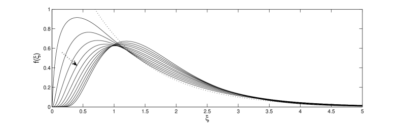
Figure 3: Similarity solutions for $s=-0.1,-0.2,...,-1$. The arrow indicates incresing values of $-s$.

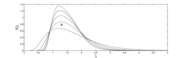
Figure 4: Similarity solutions for $s=-1,-2,...,-5$. The arrow indicates incresing values of $-s$.

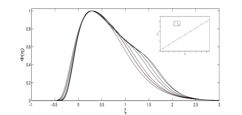
Figure 5: Rescaled similarity solutions for $-s=4,5,...,10$. Inset: value of $f_{\max}^{2}$ vs. $\left|s\right|$ and comparison with a linear law.

8 Numerical solutions of Smoluchowski equation

In this section we follow the time evolution of an arbitrary initial distribution $c_{0}$, numerically treating Smoluchowski’s equation as a differential equation of the form $\partial_{t}c\left(x,t\right)=F\left(c\left(x,t\right),x,t\right)$ with $F$ given as the right hand side of (2). Our approach has been to adopt a standard predictor-corrector, fourth order and variable time step integrator. In order to produce the numerical results, we have used almost the same scheme that was originally designed by Lee in [18]. Other authors have worked out more stable and sophisticated versions of this algorithm: we point out the recent contribution of Fibet and Laurençot [14] among them.

Let $\mathbf{x}$ be a spatially uniform grid ranging from $x_{1}=\delta_{x}$ to $x_{N}=N\delta_{x}$; we will call mass sites or mass bins $x_{k}$ following the way they are commonly referred to in the literature. When the possible mass numbers are multiples of a minimum $\delta_{x}$, Smoluchowski’s equation reduces to a discrete form:

$$\partial_{t}c\left(x_{j},t\right)=\frac{1}{2}\delta_{x}\sum_{l+k=j}K\left(x_{l},x_{k}\right)c\left(x_{l},t\right)c\left(x_{k},t\right)-c\left(x_{j},t\right)\delta_{x}\sum_{k=1}^{N}K\left(x_{j},x_{k}\right)c\left(x_{k},t\right),$$

whose right hand side can be easily computed numerically. It is also evident that this choice cuts off an infinite quantity of mass sites that, sooner or later, will become dynamically relevant in the system. To avoid this restriction, a change of variable $x\rightarrow 1/(1+x)$ was used to map the positive x-axis on the bounded interval $\left(0,1\right)$, but, as it has been clearly pointed out in [14], it is not clear how to control the distribution of the new mesh points or the mass distribution among them. See also [10] and references therein for this kind of approach.

In order to determine the cut mass $x_{N}$, our empirical criteria has been the following: given $T_{f}$ the desired ending time, if the solution has to reach a selfsimilar regime $c\left(x,t\right)\sim t^{\alpha}\psi\left(t^{\beta}x\right)$, one can find a proper value for $x$ such that $\left(T_{f}\right)^{\alpha}\psi\left(\left(T_{f}\right)^{\beta}x\right)\leq tol$, where $tol$ is a numerical parameter indicating the maximum permitted density of $x_{N}$-massed clusters at the final time; the value of $\beta$ can be taken coarsely as $\beta\sim-1-2\varepsilon,$ giving $\alpha\sim-2-4\varepsilon-4\varepsilon^{2}$ and a low accuracy $\psi$ can be computed via a previous low order simulation.

A great advantage of an uniformly distributed bin model is that the integrodifferential problem is reduced to a $N$-dimensional vector valued ordinary differential equation. Therefore, standard integration algorithms can be applied with good performances. A predictor-corrector method quickly brings an approximation of an implicit scheme, avoiding the heavy workload that computing $F\left(c\left(t,x\right),t,x\right)$ at each step would impose; it is, moreover, almost possible to guarantee the conservation of the first moment until the initial mass spreads over the $x$-line, augmenting significantly the lost mass that have reached the tail. As for the variable time step method, such an implementation is highly desirable since the peaks of variation in the distribution of $c$ tend to reduce quickly as the time passes. It is thus possible to gradually augment $\delta_{T}$ and still maintain a relative $c$-variation small enough. We refer to the huge numeric receipts literature for the reader to find further informations on those classical methods.

To compute the $N$-dimensional vector $F$ we consider all possible binary interactions $\left\{i,k\right\}$ between active bins of mass: given a small numerical threshold $\mu$, we define at each time $t$ the set $\mathbf{v}=\left\{i:c_{i}\left(t\right)\text{\textperiodcentered}x_{i}\geq\mu\right\}$. Therefore, in a cycle for $i$ ranging on $\mathbf{v}$, we consider $\mathbf{v}_{i}=\left\{k\in\mathbf{v}:k>i\right\}$ and for each pair $\left\{i,k\right\}_{k\in\mathbf{v}_{i}}$

$$F_{i}=F_{i}-\delta_{x}K\left(x_{i},x_{k}\right)c_{i}\left(t\right)c_{k}\left(t\right),\,\,\,\,\,\,\,F_{k}=F_{k}-\delta_{x}K\left(x_{i},x_{k}\right)c_{i}\left(t\right)c_{k}\left(t\right),$$ (49)

and, if $i+k\leq N$,

$$F_{i+k}=F_{i+k}+\delta_{x}K\left(x_{i},x_{k}\right)c_{i}\left(t\right)c_{k}\left(t\right).$$ (50)

Notice that we have not included the $\left\{i,i\right\}$ pair. It is also necessary to consider it, but it provides only half of the coagulating mass:

$$F_{i}=F_{i}-\delta_{x}K\left(x_{i},x_{i}\right)c_{i}^{2}\left(t\right),\,\,\,\,\,\,\,F_{2i}=F_{2i}+\frac{1}{2}\delta_{x}K\left(x_{i},x_{i}\right)c_{i}^{2}\left(t\right),\,\,\,\,\,\,\text{ if}\,\ 2i\leq N.$$ (51)

A new time step $\Delta t$ is established if the absolute variation between $c\left(x,t\right)$ and $c\left(x,t+\Delta t\right)$ is less or equal than a given tolerance. It is useful to keep track of the evolution of some relevant moments $M_{\alpha}\left(t+\Delta t\right)$. Since it is impossible to do it exactly with this finite scheme, we define some approximated values $m_{\alpha}\left(t+\Delta t\right)$ which resembles $M_{\alpha}\left(t+\Delta t\right)$, and, after each new step, we compute:

$$m_{\alpha}\left(t+\Delta t\right)=\sum_{i=1}^{N}x_{i}^{\alpha}c_{i}\left(t+\Delta t\right)+\lambda_{\alpha}\left(t+\Delta t\right),$$

where we consider an associated quantity $\lambda_{\alpha}\left(t+\Delta t\right)$ as the cumulative lost contribution to $m_{\alpha}$. It is computed in the following way: we consider again all possible binary interactions $\left\{i,k\right\}$ between active bins of mass at previous time $t$ and run a cycle for $i$ ranging on $\mathbf{v}$, but this time we look only for $\mathbf{v}_{i}^{\infty}=\left\{k\in\mathbf{v}:k>i,k+i>N\right\}$. This set takes into account only the active pairs that form clusters which exceed the cut mass $x_{N}$. Since $\delta_{x}K\left(x_{i},x_{k}\right)c_{i}\left(t\right)c_{k}\left(t\right)$ represents the velocity at which clusters of mass $x_{i+k}$ are being produced and $\Delta t$ is the interval of time that has passed, we can approximately consider that the pair $\left\{i,k\right\}$ has produced $n_{i,k}\equiv\Delta t\text{\textperiodcentered}\delta_{x}K\left(x_{i},x_{k}\right)c_{i}\left(t\right)c_{k}\left(t\right)$ new clusters of mass $x_{i+k}$. This rough estimate will only be used to compute the lost contribution to $m_{\alpha}$:

$$\lambda_{\alpha}\left(t+\Delta t\right)=\lambda_{\alpha}\left(t\right)+\sum_{i\in\mathbf{v}}\sum_{k\in\mathbf{v}_{i}^{\infty}}\left(\left(x_{i}+x_{k}\right)^{\alpha}-x_{i}^{\alpha}-x_{k}^{\alpha}\right)n_{i,k}.$$

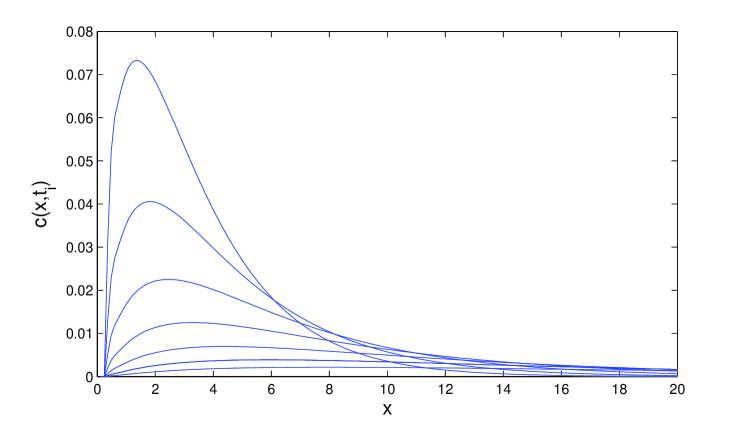
Figure 6: Solution of the evolution problem with $\varepsilon=-0.2$ for 7 different times

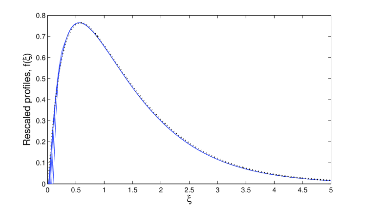
Figure 7: Rescaled profiles together with the similarity solution (dotted line).

We remark now that, from the instant when a sufficient mass escapes the finite coagulating system (infinite mass region), there are three interactions that are dynamically relevant: finite-finite, infinite-finite and infinite-infinite mass region coagulation. The former can be numerically simulated with our scheme while our knowledge of the tail distribution can only be driven forward via an ansatz (an arbitrary fast decay or a selfsimilar regime). We preferred nevertheless not to introduce such a tail into play and make the mass leaving the finite coagulating system completely stop coagulating. In that resides the need of a $x_{N}$ big enough to harbour the relevant distribution of $c$ for the solution to go as far as the self-similar regime. In Figures 6,7 we present the result of the evolution of an initial data concentrated close to the origin and for $s=-0.2$, together with the rescaled profiles. As we can see, the convergence towards the selfsimilar solution computed by the procedure described in the previous section is remarkable.

References

• [1] M. Abramowitz, I. A. Stegun, eds. (1972), Handbook of Mathematical Functions with Formulas, Graphs, and Mathematical Tables, New York: Dover Publications.
• [2] J. Banasiak, Analytic Methods for Coagulation-Fragmentation Models, Volume I (Chapman & Hall/CRC Monographs and Research Notes in Mathematics) 2019.
• [3] J. Banasiak, Analytic Methods for Coagulation-Fragmentation Models, Volume II (Chapman & Hall/CRC Monographs and Research Notes in Mathematics) 2019.
• [4] G. I. Barenblatt, Scaling, self-similarity, and intermediate asymptotics. Cambridge University Press, 1996.
• [5] G. Breschi, M. A. Fontelos, Selfsimilar solutions of the second kind representing gelation in finite time for the Smoluchowski equation, Nonlinearity 27(7), (2014), 1709–1745.
• [6] J. A. Cañizo, S. Mischler, Regularity, local behavior and partial uniqueness of self-similar profiles for Smoluchowski’s coagulation equation, Revista Matemática Iberoamericana, 27-3 (2011), 803-839.
• [7] C. Connaughton, A. C. Newell, Dynamical scaling and the finite-capacity anomaly in three-wave turbulence, Phys. Rev. E, 81, 036303 (2010).
• [8] C. Connaughton, P. L. Krapivsky, Aggregation–fragmentation processes and decaying three-wave turbulence, 81, 035303 (R) (2010).
• [9] R. L. Drake, A general mathematical survey of the coagulation equation Topics in Current Aerosol Research (Part 2) ed G M Hidy and J R Brock (Oxford: Pergamon), 1972, pp 201–376.
• [10] L. D. Erasmus, D. Eyre, and R. C. Everson, Numerical treatment of the population balance equation using a Spline-Galerkin method, Computers Chem. Engrg., 8 (1994), pp. 775–783.
• [11] M. H. Ernst, Kinetics of clustering in irreversible aggregation Fractals in Physics, ed L Pietronero and E Tosatti (Amsterdam: North-Holland), 1986, pp 289–302.
• [12] M. Escobedo, S. Mischler, Dust and self-similarity for the Smoluchowski coagulation equation, Annales de l’Institut Henri Poincare (C) Non Linear Analysis, 23(3) (2006),331-362.
• [13] M. Escobedo, S. Mischler, B. Perthame, Gelation in coagulation and fragmentation models, Comm. Math. Phys. 231 1, (2002), 157-188.
• [14] F. Filbet, P. Laurençot, Numerical Simulation of the Smoluchowski coagulation equation, SIAM J. Sci. Comput., Vol. 25 (2004), No. 6, pp. 2004-2028.
• [15] E. M. Hendriks, M. H. Ernst and R. M. Ziff, Coagulation equations with gelation, Journal of Statistical Physics 31 (1983), 519–563.
• [16] R. Jullien, R. Botet, Aggregation and Fractal Aggregates (Singapore: World Scientific) 1987.
• [17] M. H. Lee, N-body evolution of dense clusters of compact stars, Astrophys. J. 418 (1993), 147.
• [18] M. H. Lee, A survey of numerical solutions to the coagulation equation, J. Phys. A 34 10219 (2001).
• [19] F. Leyvraz, Scaling theory and exactly solved models in the kinetics of irreversible aggregation, Physics Reports 383, 2–3 (2003), 95–212.
• [20] G. Menon, G., R. L. Pego, Approach to self-similarity in Smoluchowski’s coagulation equations. Comm. Pure Appl. Math. 57 (2004), no. 9, 1197–1232.
• [21] M. Smoluchowski, Drei Vorträge über Diffusion, Brownsche Molekularbewegung und Koagulation von Kolloidteilchen, Phys Z, 17 (1916) 557–571 and 585–599.
• [22] P. G. J. van Dongen and M. H. Ernst, Dynamic Scaling in the Kinetics of Clustering, Phys. Rev. Lett. 54 (1985), 1396.
• [23] R M Ziff, M H Ernst and E M Hendriks, Kinetics of gelation and universality, J. Phys. A: Math. Gen. 16 (1983), 2293.