An Elementary but Logical Approach to Integration

Abstract.

We present a replacement for traditional Riemann integrals in undergraduate calculus, which supplements naive precalculus and at the same time opens a way to more sophisticated theories such as Lebesgue integration.

Lots of textbooks on calculus adopt traditional approaches to integration based on the so-called Riemann integral. Some authors (Bourbaki, for example) are critical in this and trying to pay much attention to linkage to the advanced theory of Lebesgue integrals, at least in the case of single variable.

For realistic applications, however, we need a naive understanding of integration in the form of an approximation by (or a limit of) a large number sum of small quantities, which should be theorefore retained in any approach.

Defects are culminated in the description of repeated calculus of improper integrals. Theoretically, integrability of multi-variable functions is required there but no practical and useful criterion is supplied in elementary courses. Thus, even if repeated integrals are possible in a safe manner, they can not be logically related to the total integrals. Of course, in Lebesgue integration, this can be dealt with by the Fubini-Tonelli theorem but at much cost for sophistication. More elementary but effective formulation is desirable even for practical integration.

We here systematically use monotone-limit extensions of elementary quadrature, which are of intermediate character in Daniell’s approach to Lebesgue integration but it works fairly well in concrete integrals and provides preliminaries to advanced theories as well with good experiences for further achievement.

The author is grateful to Amazon reviewer susumukuni for many useful comments on a draft version as well as constant impetus during the preparation of this monograph and to T. Kajiwara for illuminating discussions on the subject.

1. Sets and Functions

Set notation: Given two sets $X$ and $Y$, their product $X\times Y$ is the set of all ordered pairs $(x,y)$ ($x\in X$, $y\in Y$), $Y^{X}$ is the set of all maps of $X$ into $Y$, and the power set $2^{X}$ of $X$ is the set of all subsets of $X$. So $\text{\ym R}^{X}$ denotes the set of real-valued functions on $X$, for example.

When $X$ and $Y$ are finite sets with their numbers of elements denoted by $|X|$ and $|Y|$, we have $|X\times Y|=|X|\,|Y|$, $|Y^{X}|=|Y|^{|X|}$ and $|2^{X}|=2^{|X|}$.

Multiple products are defined in a similar fashion and identified in an associative manner: $(X\times Y)\times Z=X\times Y\times Z=X\times(Y\times Z)$. When multiple product is performed on a single set $Y$ repeatedly, $Y\times\dots\times Y$ ($n$-times repetition) is denoted by $Y^{n}$. Thus $\text{\ym R}^{n}$ denotes the set of $n$-tuples of real numbers. If $n=|X|$ with $X$ a finite set and elements of $X$ are listed by $x_{1},\dots,x_{n}$, $Y^{X}$ is naturally identified with $Y^{n}$.

Remark 1.

Throughout this monograph, the notation $|\cdot|$ is used in a multiple way: For sets, it denotes the size of its extent. For numbers and numerical vectors, it expresses the length.

Given a set $X$ and a condition $P$ on $x\in X$, we denote by $[P]$ the subset of $X$ consisting of $x\in X$ which satisfies $P$. As an example, if $f$ and $g$ are real functions on a set $X$, $[f<g]=\{x\in X;f(x)<g(x)\}$. When $P$ holds for any $x\in A$ ($A$ being a subset of $X$), i.e., $A\subset[P]$, we shall also write $P$ ($x\in A$).

The order relation in ℝ is extended to real-valued functions as well: For functions $f,g:X\to\text{\ym R}$, we write $f\leq g$ if $f(x)\leq g(x)$ ($x\in X$). It is convenient to extend the ordered set ℝ by adding formal elements $\pm\infty$ which are upper and lower bounds of ℝ respectively. This is in fact not so formal because ℝ is order isomorphic to an open interval $(-1,1)$ by a monotone bicontinuous bijection $h:\text{\ym R}\to(-1,1)$ such as $h(t)=t/(1+|t|)$ or $h(t)=(2/\pi)\arctan t$ so that the extended real line $[-\infty,\infty]$ corresponds to the closed interval $[-1,1]$.

A sequence $(f_{n})$ of real-valued functions is said to be increasing (decreasing) if $f_{n}\leq f_{n+1}$ ($f_{n}\geq f_{n+1}$) for $n\geq 1$. When $f$ is the limit function of $(f_{n})$, i.e., $\displaystyle f(x)=\lim_{n\to\infty}f_{n}(x)$ for each $x\in X$, we write $f_{n}\uparrow f$ ($f_{n}\downarrow f$).

Complex or real are used as an adjective on functions to indicate their ranges.

For a (scalar-valued) function $f$ defined on a set $X$ and a subset $A\subset X$, we make an overall use of the notation

$$\|f\|_{A}=\sup\{|f(x)|;x\in A\},$$

which satisfies the so-called seminorm condition: $\|\alpha f\|_{A}=|\alpha|\|f\|_{A}$ and $\|f+g\|_{A}\leq\|f\|_{A}+\|g\|_{A}$. When $A$ is obvious, we write simply $\|f\|$.

For a complex function $f$ defined on a set $X$, it gives rise to a map $2^{X}\to 2^{\text{\ym C}}$ by $A\mapsto\{f(a);a\in A\}$. Although logically ambiguous when both $A\subset X$ and $A\in X$ occur, it is customary to write $f(A)=\{f(a);a\in A\}$ (called the image of $A$ under $f$). Likewise a map $2^{\text{\ym C}}\to 2^{X}$ is defined by $B\mapsto f^{-1}(B)=\{x\in X;f(x)\in B\}$. Note that the inverse image $f^{-1}(B)$ of $B$ is also expressed by $[f\in B]$.

A function $f$ is said to be positive if $f(X)\subset[0,\infty)$. Thus a positive function may take $0$ as its value. If you need a function satisfying $f(x)>0$ ($x\in X$), we say that $f$ is strictly positive. Since we occasionally work with complex functions, we shall avoid ‘non-negative’ to indicate our ‘positive’.

Given a subset $A\subset X$, its indicator is a function $1_{A}$ defined by $1_{A}(x)=1$ or $0$ according to $x\in X$ or not. Thus $1_{A}\in\{0,1\}^{X}\subset\text{\ym R}^{X}$ and the correspondence $2^{X}\ni A\mapsto 1_{A}\in\{0,1\}^{X}$ is bijective.

Based on this fact, we shall identify sets and their indicators in case of no confusion.

Example 1.1.

Let $(A_{i})$ be a family of sets. Then $\sum_{i}A_{i}$ denotes a set if and only if $\bigcup_{i}A_{i}$ is a disjoint union, i.e., $\bigcup_{i}A_{i}=\bigsqcup_{i}A_{i}$.

Let $(f_{i})$ be a family of functions on a set $X$ and $\bigsqcup_{i}A_{i}\subset X$, then $\sum_{i}A_{i}f_{i}$ is a function described by

$$\Bigl{(}\sum_{i}A_{i}f_{i}\Bigr{)}(x)=\begin{cases}f_{i}(x)&\text{if $x\in A_{i}$ for some $i$,}\\ 0&\text{otherwise.}\end{cases}$$

We say that a function $f$ is supported by a set $A$ if $Af=f$.

Remark 2.

To avoid possible confusion, we prefer $Af$ to $fA$.

Exercise 1.

$A\cap B=AB=A\wedge B$, $X\setminus A=X-A$ and $A\cap B+A\cup B=A+B$.

Example 1.2.

To get more feeling on its usage and conveniency, we take up the sieve formula (the inclusion-exclusion principle) in combinatorics.

Given finitely many subsets $A_{1},\dots,A_{n}$ of $X$, de Morgan’s law is expressed by $X-(A_{1}\cup\dots\cup A_{n})=(X-A_{1})\cdots(X-A_{n})$, which is combined with its algebraic expansion

$$X-(A_{1}+\dots+A_{n})+\sum_{i<j}A_{i}\cap A_{j}+\cdots+(-1)^{n}A_{1}\cdots A_{n}$$

to obtain the identity

$$A_{1}\cup\dots\cup A_{n}=A_{1}+\dots+A_{n}-\sum_{i<j}A_{i}A_{j}+\dots+(-1)^{n-1}A_{1}\cdots A_{n}.$$

When $A_{1},\dots,A_{n}$ are all finite sets, we can evaluate these by counting measure to get to the sieve formula.

A function $f$ on a set $X$ is said to be simple if it satisfies the following equivalent conditions.

1. $f$ is a linear combination of finitely many subsets of $X$.

2. The range $f(X)$ is a finite set of scalars.

Exercise 2.

Check the equivalence of (i) and (ii).

Definition 1.3.

A real vector space $L$ consisting of real-valued functions on a set $X$ is called a linear lattice or a vector lattice if

$$f,g\in L\ \Longrightarrow\ f\vee g,f\wedge g\in L,$$

where

$$(f\vee g)(x)=\max\{f(x),g(x)\},\quad(f\wedge g)(x)=\min\{f(x),g(x)\}.$$

From the identity $2(s\diamond t)=s+t\mp|s-t|$ ($s,t\in\text{\ym R}$), the condition is equivalent to $|f|\in L$ ($f\in L$), i.e., $L$ is closed under taking absolute-value functions.

Given a linear lattice $L$, we define the positive part of $L$ by $L^{+}=\{f\in L;f\geq 0\}$, which generates $L$ linearly in view of $f=(0\vee f)+(0\wedge f)=(0\vee f)-0\vee(-f)$ ($f\in L$).

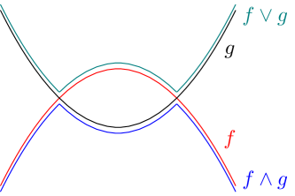
Figure 1. Lattice Operation

Definition 1.4.

A linear functional $I:L\to\text{\ym R}$ on a linear lattice $L$ is said to be positive if $I(f)\geq 0$ ($f\in L^{+}$). A positive linear functional, simply a positive functional, is continuous if $f_{n}\in L^{+}$ satisfies $f_{n}\downarrow 0$, then $I(f_{n})\downarrow 0$. A continuous positive functional is called a preintegral (or a Daniell integral).

An integral system on a set $X$ is defined to be a couple $(L,I)$ of a linear lattice $L$ on $X$ and a preintegral $I$ on $L$.

Exercise 3.

A linear functional $I$ on a linear lattice $L$ is positive if and only if $|I(f)|\leq I(|f|)$ ($f\in L$).

By a division in a set $X$, we shall mean a finite family 𝒟 of mutually disjoint non-empty subsets of $X$ and, given a division 𝒟, let $\text{\ym R}{\hbox{\sy D}}=\sum_{D\in{\hbox{\sy D}}}\text{\ym R}D$ be the set of linear combinations of sets in 𝒟, which is an algebra and a linear lattice at the same time (called an algebra-lattice). The algebra ℝ𝒟 has a unit element given by $[{\hbox{\sy D}}]=\bigsqcup_{D\in{\hbox{\sy D}}}D$ (called the support of 𝒟).

Since 𝒟 is linearly independent as a family in ℝ𝒟, the vector space ℝ𝒟 is naturally isomorphic to $\text{\ym R}^{\hbox{\sy D}}$ as an algebra-lattice and any positive function $\mu$ on 𝒟 is extended to a positive functional $I$ on ℝ𝒟, which is obviously continuous. Thus there is a one-to-one correspondence (by restriction and extension) between positive functions on 𝒟 and preintegrals on ℝ𝒟.

Among divisions in $X$, we define an order relation ${\hbox{\sy D}}\prec{\hbox{\sy E}}$ by $\text{\ym R}{\hbox{\sy D}}\subset\text{\ym R}{\hbox{\sy E}}$, which is equivalently described by the condition that each $D\in{\hbox{\sy D}}$ is a disjoint union of $E\in{\hbox{\sy E}}$ included in $D$. We say that ℰ is a subdivision of 𝒟 if ${\hbox{\sy D}}\prec{\hbox{\sy E}}$ and $[{\hbox{\sy D}}]=[{\hbox{\sy E}}]$. Let $I$ and $J$ be preintegrals on ℝ𝒟 and ℝℰ respectively. Then $J$ is an extension of $I$ if and only if they are related by $I(D)=\sum_{E\subset D}J(E)$ ($D\in{\hbox{\sy D}}$, $E\in{\hbox{\sy E}}$).

We assume and follow standard terminology and notations on the topology in $\text{\ym R}^{d}$. For example, given a subset $D\subset\text{\ym R}^{d}$, $\partial D$ denotes the boundary of $D$. Non-standard is the notation and the meaning for the support of a function $f$ defined on a subset $A$ of $\text{\ym R}^{d}$: The closure of $[f\not=0]$ in $\text{\ym R}^{d}$ is called the support of $f$ and is denoted by $[f]$. In other words, our support of $f$ is the ordinary support of the zero extension of $f$ to $\text{\ym R}^{d}$.

For a subset $A$ of $\text{\ym R}^{d}$, $C(A)$ denotes the set of continuous functions on $A$. When $A$ is open, a continuous function $f\in C(A)$ is said to have a compact support if $[f]$ is bounded and $[f]\subset A$. The set of continuous functions on $A$ having compact supports is denoted by $C_{c}(A)$.

2. Definite and Indefinite Integrals

Here we discuss definite integrals of functions of a single variable.

A step function is by definition a linear combination of bounded intervals in ℝ. Let $S(\text{\ym R})$ be the linear space of step functions. For a bounded interval $D$ with $a\leq b$ endpoints, its width (or length) $b-a$ is denoted by $|D|$.

Given a finite partition $\Delta=\{t_{0}<t_{1}<\dots<t_{n}\}$ in ℝ, open intervals $(t_{0},t_{1}),\dots,(t_{n-1},t_{n})$ together with one-point intervals $[t_{0},t_{0}],\dots,[t_{n},t_{n}]$ (called interval parts) are linearly independent in $S(\text{\ym R})$ and, if we denote by $\text{\ym R}\Delta$ the set of their linear spans, $\text{\ym R}\Delta$ is an algebra-lattice with the width function on interval parts in $\Delta$ linearly extended to a positive linear functional $I_{\Delta}$. It is immediate to see that if $\Delta^{\prime}$ is a refinement of $\Delta$, then $\text{\ym R}\Delta\subset\text{\ym R}\Delta^{\prime}$ and $I_{\Delta^{\prime}}$ extends $I_{\Delta}$.

Given finitely many intervals $D_{1},\dots,D_{m}$, we can find a finite partition $\Delta$ so that each $D_{j}$ is a sum of interval parts in $\Delta$. Note that $D_{j}\Delta_{i}=\Delta_{i}$ or $0$ according to $\Delta_{i}\subset D_{j}$ (denoted by $i\prec j$) or not. Moreover we have an expression $D_{j}=\sum_{i\prec j}\Delta_{i}$ together with an obvious equality $|D_{j}|=\sum_{i\prec j}|\Delta_{i}|$.

Lemma 2.1.

The step function space $S(\text{\ym R})$ is an algebra-lattice. The width function is extended to a positive linear functional $I$ on $S(\text{\ym R})$, which is referred to as the width integral.

Proof.

Since interval parts in $\Delta$ are idempotents in the function algebra $\text{\ym R}^{\text{\ym R}}$, their linear combinations constitute an algebra-lattice, which is inherited from $S(\text{\ym R})$.

To see that the width function is well-extended to a positive linear functional, let $\sum_{j}\alpha_{j}D_{j}=\sum_{k}\beta_{k}E_{k}$ with $D_{j}$ and $E_{k}$ bounded intervals. Choose a partition $\Delta$ so that $D_{j},E_{k}\in\text{\ym R}\Delta$. Then

$$\sum_{j}\alpha_{j}|D_{j}|=\sum_{i\prec j}\alpha_{j}|\Delta_{i}|=I_{\Delta}(\sum_{j}\alpha_{j}D_{j})\\ =I_{\Delta}(\sum_{k}\beta_{k}E_{k})=\sum_{i\prec k}\beta_{k}I_{\Delta}(\Delta_{i})=\sum_{k}\beta_{k}|E_{k}|.$$

∎

The width function is now extended to a set $A\in S(\text{\ym R})$ by $|A|=I(A)$. Note that such an $A$ is exactly a union of finitely many bounded intervals. The following is a key toward integral extensions.

Lemma 2.2.

Let $\bigsqcup_{n\geq 1}D_{n}$ be a decomposition of an open interval $(a,b)$ into countably many bounded intervals. Then $b-a=\sum_{n=1}^{\infty}|D_{n}|$.

Proof.

Intuitively this seems obvious because it just prevents infinitesimal leakage from the summation and you may take it for granted to see further developments. The proof itself is, however, not difficult once you know the Heine-Borel covering theorem:

Since $\sum_{j=1}^{n}D_{j}\leq(a,b)$ as functions on ℝ, taking the width integral gives $\sum_{j=1}^{n}|D_{j}|\leq b-a$ and then $\sum_{n\geq 1}|D_{n}|\leq b-a$.

To get the reverse inequality, given $\epsilon>0$, by replacing each $D_{n}$ with a slightly large open interval $U_{n}$ satisfying $|U_{n}|\leq|D_{n}|+\epsilon/2^{n}$, we consider an open covering $(U_{n})$ of $[a+\epsilon,b-\epsilon]$ and can find a finite subcover $(U_{n_{j}})_{1\leq j\leq k}$ by the Heine-Borel (A.1) so that

$$[a+\epsilon,b-\epsilon]\leq\bigcup_{j=1}^{k}U_{n_{j}}\leq\sum_{j=1}^{k}U_{n_{j}}$$

is evaluated by the width integral to get

$$b-a-2\epsilon\leq\sum_{j=1}^{k}|U_{n_{j}}|\leq\sum_{n\geq 1}|U_{n}|\leq\sum_{n\geq 1}|D_{n}|+\sum_{n\geq 1}\frac{\epsilon}{2^{n}}=\sum_{n\geq 1}|D_{n}|+\epsilon.$$

Thus $b-a\leq\sum_{n\geq 1}|D_{n}|+3\epsilon$. ∎

Corollary 2.3.

Monotone continuity holds for the width integral.

Proof.

We first claim that, if $\bigsqcup_{n\geq 1}A_{n}$ is a decomposition of a set $A\in S(\text{\ym R})$ into $A_{n}\in S(\text{\ym R})$, then $|A|=\sum_{n=1}^{\infty}|A_{n}|$. In fact, $A$ is a finite disjoint union of open intervals $(a,b)$ and points. For points, the width integral satisifes the equality by $0=\sum_{n}0$ and, for open intervals, the assertion in the lemma gives $|(a,b)|=\sum_{n}|(a,b)\cap A_{n}|$. (Note here that $(a,b)\cap A_{n}$ is a disjoint union of finitely many bounded intervals.) Summing these up, we obtain the claim.

Let $(h_{n})_{n\geq 1}$ be a decreasing sequence of step functions satisfying $h_{n}\downarrow 0$. We show that the width integral satisfies $I(h_{n})\downarrow 0$.

Since both $[h_{1}>0]$ and $[h_{n}\leq\epsilon]h_{n}$ are step functions and satisfy $[h_{n}\leq\epsilon]h_{n}\leq[h_{1}>0]\epsilon$ for any $\epsilon>0$, evaluation by the width integral gives

$$I(h_{n})=I([h_{n}\leq\epsilon]h_{n})+I([h_{n}>\epsilon]h_{n})\leq\epsilon|[h_{1}>0]|+\|h_{1}\||[h_{n}>\epsilon]|$$

and the continuity is reduced to showing $\Bigl{|}[h_{n}>\epsilon]\Bigr{|}\downarrow 0$ as $n\to\infty$.

To see this, we rewrite $[h_{n}>\epsilon]\downarrow\emptyset$ into the form

$$[h_{m}>\epsilon]=\bigsqcup_{n\geq m}\Bigl{(}[h_{n}>\epsilon]\setminus[h_{n+1}>\epsilon]\Bigr{)}=\bigsqcup_{n\geq m}[h_{n}>\epsilon]\cap[h_{n+1}\leq\epsilon]$$

for any $m\geq 1$. Since $[h_{n}>\epsilon]$ and $[h_{n}>\epsilon]\cap[h_{n+1}\leq\epsilon]$ belong to $S(\text{\ym R})$, we can apply the above claim to have

$$\Bigl{|}[h_{m}>\epsilon]\Bigr{|}=\sum_{n\geq m}\Bigl{|}[h_{n}>\epsilon]\cap[h_{n+1}\leq\epsilon]\Bigr{|},$$

which approaches $0$ as $m\to\infty$ because $\sum_{n\geq 1}\Bigl{|}[h_{n}>\epsilon]\cap[h_{n+1}\leq\epsilon]\Bigr{|}=|h_{1}>\epsilon]|<\infty$. ∎

Thus the width integral on step functions is a preintegral and gives an integral system on ℝ.

To know how the above reassembling lemma is non-trivial, consider the following generalization due to Stieltjes: Let $\phi:\text{\ym R}\to\text{\ym R}$ be a (weakly) increasing function. Remark first that jumping points $c$ satisfying $\phi(c-0)<\phi(c+0)$ are countable because given a finite interval $[a,b]$ $\{c\in[a,b];\phi(c+0)-\phi(c-0)\geq 1/n\}$ is a finite set for every $n=1,2,\dots$. Now the Stieltjes mass is assigned to finite interval parts by

$$|(a,b)|_{\phi}=\phi(b-0)-\phi(a+0),\quad|\{c\}|_{\phi}=\phi(c+0)-\phi(c-0)$$

and linearly extended to a positive functional $I_{\phi}$ on $S(\text{\ym R})$, which is called the Stieltjes integral. Note here that values at jumping points are irrelevant in this construction and it is customary to impose left or right continuity on $\phi$ so that $\phi$ is uniquely determined from the Stieltjes integral.

We here claim that, given a partition $R=\sqcup R_{j}$ of a bounded interval $R$ into a countable sequence $(R_{j})$ of bounded intervals,

$$|R|_{\phi}=\sum_{j}|R_{j}|_{\phi}.$$

Again non-trivial is the inequality $|R|_{\phi}\leq\sum_{j}|R_{j}|_{\phi}$.

For a bounded non-open interval, we can move boundary points slightly outer to make it open but the Stieltjes mass difference remain small. This is possible from the limiting definition of the Stieltjes mass: Given $\epsilon>0$, let $R_{j}^{\epsilon}$ be an open interval including $R_{j}$ and satisfying $|R_{j}^{\epsilon}|_{\phi}\leq|R|_{\phi}+\epsilon/2^{j}$ (we may take $R_{j}^{\epsilon}=R_{j}$ if $R_{j}$ is open).

First consider $R=[a,b]$. By the Heine-Borel covering theorem (A.1), for a sufficently large $n\geq 1$, $R\subset\bigcup_{j=1}^{n}R_{j}^{\epsilon}\leq\sum_{j=1}^{n}R_{j}^{\epsilon}$ and hence

$$|R|_{\phi}=I_{\phi}(R)\leq\sum_{j=1}^{n}I_{\phi}(R_{j}^{\epsilon})=\sum_{j=1}^{n}|R_{j}^{\epsilon}|_{\phi}\leq\sum_{j=1}^{n}(|R_{j}|_{\phi}+\epsilon/2^{j})\leq\sum_{j=1}^{n}|R_{j}|_{\phi}+\epsilon.$$

Thus the cliam holds. Since $\epsilon>0$ is arbitrary, this gives $|R|_{\phi}\leq\sum_{j}|R_{j}|_{\phi}$.

When $R=(a,b)$, add $\{a\}$, $\{b\}$ to $(R_{j})$ and apply the reassembling formula for $[a,b]$ to have

$$|\{a\}|_{\phi}+|\{b\}|_{\phi}+|(a,b)|_{\phi}=|[a,b]|_{\phi}=|\{a\}|_{\phi}+|\{b\}|_{\phi}+\sum_{j=1}^{\infty}|R_{j}|_{\phi},$$

which shows that the claim is true for $R=(a,b)$. Similarly for $R=(a,b]$ and $R=[a,b)$.

Once the reassembling formula for mass is established, we can repeat the argument in Corollary 2.3 to see that $I_{\phi}$ is continuous, i.e., the Stieltjes integral is a preintegral on $S(\text{\ym R})$.

Remark 3.

In contrast to Stieltjes integrals, values on finitely many points are irrelevant in the width integral. Based on this fact, it is often convenient to work with open-closed intervals (or closed-open intervals) instead of full intervals as witnessed in the Cauchy-Riemann-Darboux approach below.

Next we enlarge a linear lattice $L$ by monotone sequential limits as a preparation to integral extensions.

Definition 2.4.

Given a linear lattice $L$ on $X$, we set

$$L_{\uparrow} =\{f:X\to(-\infty,\infty];\exists\,\text{a sequence}f_{n}\in L,f_{n}\uparrow f\},$$

$$L_{\downarrow} =\{f:X\to[-\infty,\infty);\exists\,\text{a sequence}f_{n}\in L,f_{n}\downarrow f\}$$

and $L_{\uparrow}^{+}=\{f\in L_{\uparrow};f\geq 0\}$. Functions in $L_{\uparrow}$ ($L_{\downarrow}$) are referred to as upper (lower) functions respectively.

Notice that any monotone sequence $(f_{n})$ in $L$ has a limit in $L_{\updownarrow}$, where the notation $L_{\updownarrow}$ is used to stand for $L_{\uparrow}$ or $L_{\downarrow}$. For $L=S(\text{\ym R})$, we write $S_{\updownarrow}(\text{\ym R})$ instead of $L_{\updownarrow}$.

The following are immediate from these definitions.

Proposition 2.5.

1. $L_{\downarrow}=-L_{\uparrow}$ and $L\subset L_{\uparrow}\cap L_{\downarrow}$.

2. $L_{\updownarrow}$ are semilinear lattices in the sense that, for $\alpha,\beta\in\text{\ym R}_{+}$ and $f,g\in L_{\updownarrow}$, we have $\alpha f+\beta g,f\vee g,f\wedge g\in L_{\updownarrow}$. Consequently $L_{\uparrow}\cap L_{\downarrow}$ is a linear lattice.

3. Moreover if $L$ is an algebra (i.e., being closed under multiplication), $L_{\updownarrow}^{+}L_{\updownarrow}\subset L_{\updownarrow}$ and $L_{\uparrow}\cap L_{\downarrow}$ is also an algebra.

Exercise 4.

Check the above properties on $L_{\updownarrow}$.

We say that a function $f:\text{\ym R}\to\text{\ym R}$ is doubly bounded if it is bounded and has a bounded support.

Lemma 2.6.

1. For $f\in S_{\updownarrow}(\text{\ym R})$, $0\wedge(\pm f)$ is doubly bounded. Consequently functions in $S_{\uparrow}(\text{\ym R})\cap S_{\downarrow}(\text{\ym R})$ are doubly bounded as well.

2. A function $f:\text{\ym R}\to[0,\infty)$ belongs to $S_{\uparrow}(\text{\ym R})$ if it is continuous on an open interval $(a,b)$ and satisifies $(a,b)f=f$. Here $-\infty\leq a<b\leq\infty$.

Proof.

Non-trivial is (ii). Choose $a_{n}\downarrow a$ and $b_{n}\uparrow b$ so that $[a_{n},b_{n}]\subset(a,b)$. Dividing $(a,b]$ into subintervals finer and finer, we can find an increasing double sequence $f_{n,k}$ in $S^{+}(\text{\ym R})$ so that $f_{n,k}=(a_{n},b_{n}]f_{n+1,k}$, $f_{n,k}\leq f_{n,k+1}$ and $\displaystyle\lim_{k\to\infty}f_{n,k}=(a_{n},b_{n}]f$ thanks to the Darboux approximation (see Cauchy-Riemann-Darboux approach at the end of this section) based on uniform continuity of $[a_{n},b_{n}]f$.

Now the diagonal sequence $f_{n}=f_{n,n}$ in $S^{+}(\text{\ym R})$ satisfies $f_{n}\uparrow f$ and we are done. ∎

Corollary 2.7.

If $f$ is a doubly bounded function having finitely many points of discontinuity, then $f\in S_{\uparrow}(\text{\ym R})\cap S_{\downarrow}(\text{\ym R})$.

Proof.

By assumption, we can choose a partition $a=t_{0}<t_{1}<\cdots<t_{l}=b$ so that $(a,b)f=f$ and the points of discontinuity of $f$ are contained in $\{t_{0},\dots,t_{n}\}$. Then, in the expression

$$(a,b)(f+\|f\|)=\sum_{j=0}^{l-1}(t_{j},t_{j+1})(f+\|f\|)+\sum_{j=0}^{l}[t_{j},t_{j}](\|f\|+f_{j}),$$

we apply (ii) to see that it belongs to $S_{\uparrow}(\text{\ym R})$, whence $f\in S_{\uparrow}(\text{\ym R})$ as a sum of $(a,b)(f+\|f\|)$ and $-(a,b)\|f\|\in S(\text{\ym R})\subset S_{\uparrow}(\text{\ym R})$.

Likewise, $-f\in S_{\uparrow}(\text{\ym R})$, i.e., $f\in S_{\downarrow}(\text{\ym R})$. ∎

Lots of functions belong to $S_{\uparrow}\cup S_{\downarrow}$ but of course not always.

Example 2.8.

1. We see $(0,r)\bigl{(}\pm 1+\sin(1/x)\bigr{)}\in S_{\updownarrow}(\text{\ym R})$ for $0<r\leq\infty$ and then $(0,r)\sin(1/x)\in S_{\uparrow}(\text{\ym R})\cap S_{\downarrow}(\text{\ym R})$ for $0<r<\infty$.

2. Let $C$ be a dense subset of an open (non-empty) interval $(a,b)$ and assume that $(a,b)\setminus C$ is also dense in $(a,b)$. Then neither $S_{\uparrow}(\text{\ym R})$ nor $S_{\downarrow}(\text{\ym R})$ contains $C$ as an indicator function.

   In fact, let $(f_{n})$ be a decreasing sequence in $S(\text{\ym R})$ satisfying $C\leq f_{n}$ ($n\geq 1$). Since $f_{n}$ is continuous except for finitely many points, the density of $C\in(a,b)$ is used to see $f_{n}\geq(a,b)\geq C$ but $C\not=(a,b)$, showing $C\not=\lim f_{n}$ and hence $C\not\in S_{\downarrow}(\text{\ym R})$.

   Likewise, $(a,b)\setminus C\not\in S_{\downarrow}(\text{\ym R})$, i.e., $C-(a,b)=-((a,b)\setminus C)\not\in S_{\uparrow}(\text{\ym R})$ and then $C=(a,b)+(C-(a,b))\not\in S_{\uparrow}(\text{\ym R})$ in view of $(a,b)\in S(\text{\ym R})$.

3. Both $\sin x$ and $x/(1+|x|)$ do not belong to $S_{\uparrow}(\text{\ym R})\cup S_{\downarrow}(\text{\ym R})$ simply because their positive and negative parts are unbounded.

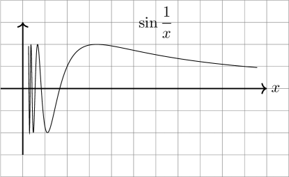
Figure 2. Rapid Oscillation

Exercise 5.

Any countable dense subset of $(a,b)$ satisfies the condition in (ii). Hint: $(a,b)$ is not countable.

Exercise 6.

For a sequence $(a_{n})$ satisfying $a_{n}>a_{n+1}$ ($n\geq 1$) and $a_{n}\downarrow 0$, show that a comb function $\displaystyle\sum_{n\geq 1}[a_{2n},a_{2n-1}]$ is in $S_{\uparrow}(\text{\ym R})\cap S_{\downarrow}(\text{\ym R})$.

Exercise 7.

A monotone (increasing or decreasing) function $f:\text{\ym R}\to[-\infty,\infty]$ belongs to $S_{\updownarrow}(\text{\ym R})$ if and only if $\pm f\geq 0$. Hint: Level approximation in Appendix C.

Remark 4.

We notice that so many functions belong to “$S_{\uparrow}(\text{\ym R})-S_{\downarrow}(\text{\ym R})$” but a big issue here is that $f_{\uparrow}-f_{\uparrow}$ ($f_{\updownarrow}\in S_{\updownarrow}(\text{\ym R})$) is not always well-defined due to the possibility $\infty-\infty$. Later we discuss a remedy for this.

We shall now extend a preintegral $I$ from $L$ to $L_{\updownarrow}$.

Lemma 2.9.

Let $(f_{n})$, $(g_{n})$ be increasing sequence in a linear lattice $L$ satisfying the inequality

$$\lim_{n}f_{n}\leq\lim_{n}g_{n}$$

for $(-\infty,\infty]$-valued limit functions (neither $\lim_{n}f_{n}$ nor $\lim_{n}g_{n}$ being assumed to be in $L$). Then we have

$$\lim_{n}I(f_{n})\leq\lim_{n}I(g_{n}).$$

Proof.

From the assumption, $f_{m}\leq\lim_{n\to\infty}g_{n}$ and hence $f_{m}=\lim_{n\to\infty}f_{m}\wedge g_{n}$. By applying the continuity of $I$ to $(f_{m}-f_{m}\wedge g_{n})\downarrow 0$, we have

$$I(f_{m})=\lim_{n\to\infty}I(f_{m}\wedge g_{n})\leq\lim_{n\to\infty}I(g_{n})$$

and the limit on $m$ gives the assertion. ∎

Definition 2.10.

The previous lemma allows us to define a functional $I_{\uparrow}:L_{\uparrow}\to(-\infty,\infty]$ by

$$I_{\uparrow}(f)=\lim_{n\to\infty}I(f_{n}),\quad f_{n}\uparrow f,\ f_{n}\in L.$$

Likewise, $I_{\downarrow}:L_{\downarrow}\to[-\infty,\infty)$ is defined by

$$I_{\downarrow}(f)=\lim_{n\to\infty}I(f_{n}),\quad f_{n}\downarrow f,\ f_{n}\in L.$$

Here are immediate properties of these extensions:

Proposition 2.11.

1. $I_{\downarrow}(-f)=-I_{\uparrow}(f)$ for $f\in L_{\uparrow}$ (recall that $-L_{\uparrow}=L_{\downarrow}$).

2. Functionals $I_{\uparrow}$ and $I_{\downarrow}$ coincide on $L_{\uparrow}\cap L_{\downarrow}$ and extend $I$, i.e., $I_{\uparrow}(f)=I_{\downarrow}(f)\in\text{\ym R}$ for $f\in L_{\uparrow}\cap L_{\downarrow}$ and $L_{\uparrow}(f)=I(f)=I_{\downarrow}(f)$ for $f\in L$.

3. Functionals $I_{\uparrow}$ and $I_{\downarrow}$ are semilinear, i.e., for $\alpha,\beta\in\text{\ym R}_{+}$ and $f,g\in L_{\updownarrow}$,

   $$I_{\updownarrow}(\alpha f+\beta g)=\alpha I_{\updownarrow}(f)+\beta I_{\updownarrow}(g).$$

4. If $f,g\in L_{\updownarrow}$ satisfy $f\leq g$, then $I_{\updownarrow}(f)\leq I_{\updownarrow}(g)$.

Thus $I_{\updownarrow}$ ($I_{\uparrow}$ or $I_{\downarrow}$) is a positive functional on the linear lattice $L_{\uparrow}\cap L_{\downarrow}$.

Proof.

We just indicate the coincidence in (ii): If $g_{n}\uparrow f$ and $h_{n}\downarrow f$ with $g_{n},h_{n}\in L$, then $h_{n}-g_{n}\downarrow 0$ and hence $I(h_{n})-I(g_{n})\downarrow 0$ by continuity of $I$. Thus $I_{\uparrow}(f)=\lim I(g_{n})=\lim I(h_{n})=I_{\downarrow}(f)$. ∎

Exercise 8.

Check other properties.

The monotone extensions are now applied to the width integral, which are conventionally denoted by

$$\int f(t)\,dt\in\text{\ym R}\cup\{\pm\infty\}\quad(f\in S_{\updownarrow}(\text{\ym R})).$$

Here arises no ambiguity thanks to the coincidence $I_{\uparrow}=I_{\downarrow}$ on $S_{\uparrow}(\text{\ym R})\cap S_{\downarrow}(\text{\ym R})$. Note that it gives a positive linear functional on $S_{\uparrow}(\text{\ym R})\cap S_{\downarrow}(\text{\ym R})$.

Now let $f:\text{\ym R}\to\text{\ym R}$ satisfy $[a,b]f\in S_{\uparrow}(\text{\ym R})\cap S_{\downarrow}(\text{\ym R})$. The integral of $[a,b]f$ is called the definite integral of $f$ on $[a,b]$ and denoted by

$$\int_{a}^{b}f(t)\,dt.$$

The definite integral is clearly linear and monotone in $f$, whence it satisfies the integral inequality:

$$\left|\int_{a}^{b}f(t)\,dt\right|\leq\int_{a}^{b}|f(t)|\,dt\leq(b-a)\|f\|_{[a,b]}.$$

Consequently, if a sequence $(f_{n})$ and $f$ satisfy $[a,b]f_{n}\in S_{\uparrow}(\text{\ym R})\cap S_{\downarrow}(\text{\ym R})$, $[a,b]f\in S_{\uparrow}(\text{\ym R})\cap S_{\downarrow}(\text{\ym R})$ and $[a,b]f_{n}\to[a,b]f$ uniformly on $[a,b]$, then

$$\lim_{n\to\infty}\int_{a}^{b}f_{n}(t)\,dt=\int_{a}^{b}f(t)\,dt.$$

In the definition of definite integral, we may use other types of intervals, say $(a,b]$, as well because functions supported by finite sets belong to $S_{\uparrow}(\text{\ym R})\cap S_{\downarrow}(\text{\ym R})$ with their integrals equal to zero.

The definite integral is additive on supporting intervals: If $a\leq c\leq b$, $[a,b]f\in S_{\uparrow}(\text{\ym R})\cap S_{\downarrow}(\text{\ym R})$ if and only if $[a,c]f$ and $[c,b]f$ belong to $S_{\uparrow}(\text{\ym R})\cap S_{\downarrow}(\text{\ym R})$. Moreover, if this is the case, we have

$$\int_{a}^{b}f(t)\,dt=\int_{a}^{c}f(t)\,dt+\int_{c}^{b}f(t)\,dt.$$

In accordance with this additivity, it is then customary to write

$$\int_{b}^{a}f(t)\,dt=-\int_{a}^{b}f(t)\,dt.$$

Example 2.12.

1. Any function $f$ which is continuous on $[a,b]$ admits the definite integral $\int_{a}^{b}f(t)\,dt$ by Corollary 2.7.

2. For $r\in\text{\ym R}$, the translated function $g(t)=f(t-r)$ satisfies $[a+r,b+r]g\in S_{\uparrow}(\text{\ym R})\cap S_{\downarrow}(\text{\ym R})$ if and only if $[a,b]f\in S_{\uparrow}(\text{\ym R})\cap S_{\downarrow}(\text{\ym R})$, and in this case

   $$\int_{a}^{b}f(t)\,dt=\int_{a+r}^{b+r}f(t-r)\,dt.$$

Example 2.13.

Let $f(t)=\sin(1/t)$ for $t\not=0$ and assign any value at $t=0$. Then $[a,b]f\in S_{\uparrow}(\text{\ym R})\cap S_{\downarrow}(\text{\ym R})$ for every bounded $[a,b]\subset\text{\ym R}$ by Corollary 2.7 and the definite integral $\int_{a}^{b}f(t)\,dt$ is well-defined.

Exercise 9.

For $r>0$, $[ra,rb]f\in S_{\uparrow}(\text{\ym R})\cap S_{\downarrow}(\text{\ym R})$ if and only if the scaled function $g(t)=f(rt)$ satisfies $[a,b]g\in S_{\uparrow}(\text{\ym R})\cap S_{\downarrow}(\text{\ym R})$. Moreover, if this is the case,

$$\int_{a}^{b}f(rt)\,dt=\frac{1}{r}\int_{ra}^{rb}f(t)\,dt.$$

Now an indefinite integral of $f$ is a function of $x$ defined by

$$\int_{a}^{x}f(t)\,dt$$

with $a$ a preassigned point and $x\in\text{\ym R}$ satisfying $[a,x]f\in S_{\uparrow}(\text{\ym R})\cap S_{\downarrow}(\text{\ym R})$. The difference of indefinite integrals is therefore a constant function and indefinite integrals of $f$ are determined up to additive constants.

Example 2.14.

For a function $f\in S_{\uparrow}(\text{\ym R})\cap S_{\downarrow}(\text{\ym R})$, the indefinite integral $\displaystyle\int_{a}^{x}f(t)\,dt$ is everywhere defined for any $a\in\text{\ym R}$ and is locally constant outside the support $[f]$ of $f$. In particular, the indefinite integral is constant for a sufficiently large $|x|$.

The following, known as the fundamental theorem in calculus, is literally of fundamental importance.

Theorem 2.15.

An indefinite integral is a continuous function and, if $f(t)$ is continuous at $t=c$, it is differentiable at $x=c$ in such a way that

$$\frac{d}{dx}\int_{a}^{x}f(t)\,dt=f(c).$$

Proof.

Continuity of an indefinite integral of $f$ follows from the integral inequality

$$\left|\int_{x}^{y}f(t)\,dt\right|\leq|x-y|\|f\|_{[x,y]}$$

in view of local boundedness of $f$.

For $\delta>0$, if $x$ satisfies $|x-c|\leq\delta$,

$$\left|\frac{1}{x-c}\left(\int_{a}^{x}f(t)\,dt-\int_{a}^{c}f(t)\,dt\right)-f(c)\right| =\left|\frac{1}{x-c}\int_{c}^{x}(f(t)-f(c))\,dt\right|$$

$$\leq\|f-f(c)\|_{[c-\delta,c+\delta]},$$

which converges to $0$ as $\delta\to+0$ by continuity of $f(x)$ at $x=c$. ∎

Corollary 2.16.

If $f$ is continuous on an open interval $(a,b)$, it admits a primitive function $F$ in such a way that

$$\int_{x}^{y}f(t)\,dt=F(y)-F(x)\equiv\bigl{[}F(t)\bigr{]}_{x}^{y}$$

for any $[x,y]\subset(a,b)$.

Recall that a primitive function of a function $f$ defined on an open interval $(a,b)$ is a differentiable function $F$ on $(a,b)$ satisfying $F^{\prime}=f$. Also recall that primitive functions of $f$ are unique up to additive constants.

Proof.

As functions of $y$ ($x$ being fixed), both sides are primitive functions of $f$ and coincide at $y=x$. ∎

Example 2.17.

For $\alpha\geq 0$, consider a function $f_{\alpha}(t)$ of $t\in\text{\ym R}$ defined by

$$f_{\alpha}(t)=\begin{cases}t^{\alpha}&(t>0),\\ 0&(t\leq 0),\end{cases}$$

which is continuous for $\alpha>0$ but has discontinuity at $t=0$ for $\alpha=0$. In either case, indefinite integrals are defined everywhere and given by continuous functions

$$\int_{0}^{x}f_{\alpha}(t)\,dt=\begin{cases}x^{\alpha+1}/(\alpha+1)&(x>0),\\ 0&(x\leq 0),\end{cases}$$

which are differentiable and give primitive functions of $f_{\alpha}$ for $\alpha>0$ but not for $\alpha=0$ (no primitive function of $f_{0}$ exists).

Let a function $f:(a,b)\to\text{\ym R}$ satisfy $[x,y]f\in S_{\uparrow}(\text{\ym R})\cap S_{\downarrow}(\text{\ym R})$ for $a<x\leq y<b$. An improper integral of $f$ is defined to be

$$\int_{a}^{b}f(t)\,dt=\lim_{(x,y)\to(a,b)}\int_{x}^{y}f(t)\,dt=\lim_{x\to a+0}\int_{x}^{c}f(t)\,dt+\lim_{y\to b-0}\int_{c}^{y}f(t)\,dt$$

if limits exist. When $f\in S_{\uparrow}(\text{\ym R})\cap S_{\downarrow}(\text{\ym R})$ and $(a,b)$ is bounded, it is reduced to the definite integral $\int_{a}^{b}f(t)\,dt$. Improperly integrable functions constitute a linear space with the improper integral giving a positive functional but improperly integrable functions do not form a lattice.

Related to this fact, we say that a function $f:(a,b)\to\text{\ym R}$ is absolutely convergent if $[x,y]f\in S_{\uparrow}(\text{\ym R})\cap S_{\downarrow}(\text{\ym R})$ and $|f|$ is improperly integrable. In that case, $f$ is improperly integrable and satisfies the integral inequality

$$\left|\int_{a}^{b}f(x)\,dx\right|\leq\int_{a}^{b}|f(x)|\,dx.$$

An improper integral is said to be conditionally convergent if it is not absolutely convergent.

Later we shall see that absolutely convergent integrals are properly extended to multiple integrals.

Proposition 2.18 (Frullani integral).

Let a function $f:(0,\infty)\to\text{\ym R}$ satisfy $[x,y]f\in S_{\uparrow}(\text{\ym R})\cap S_{\downarrow}(\text{\ym R})$ for $0<x\leq y<\infty$ and assume that $f(0)=\lim_{t\to+0}f(t)$ and $f(\infty)=\lim_{t\to\infty}f(t)$ exist. Then, for $0<a<b$, the function $\frac{f(bt)-f(at)}{t}$ is improperly integrable on $(0,\infty)$ and

$$\int_{0}^{\infty}\frac{f(bt)-f(at)}{t}\,dt=\Bigl{(}f(\infty)-f(0)\Bigr{)}\log\frac{b}{a}.$$

Note here that $f(at)/t$ ($x\leq t\leq y$) belongs to $S_{\uparrow}(\text{\ym R})\cap S_{\downarrow}(\text{\ym R})$.

Proof.

Take $x>0$ small and $y\geq x$ large. Then from the scaling invariance of $dt/t$ (Exercise 9), we have

$$\int_{x}^{y}\frac{f(bt)-f(at)}{t}\,dt =\int_{bx}^{by}\frac{f(t)}{t}\,dt-\int_{ax}^{ay}\frac{f(t)}{t}\,dt$$

$$=\int_{ay}^{by}\frac{f(t)}{t}\,dt-\int_{ax}^{bx}\frac{f(t)}{t}\,dt$$

$$=\int_{a}^{b}\frac{f(ty)}{t}\,dt-\int_{a}^{b}\frac{f(tx)}{t}\,dt.$$

Since $\displaystyle\lim_{y\to\infty}f(ty)=f(\infty)$ and $\displaystyle\lim_{x\to+0}f(tx)=f(0)$ uniformly in $t\in[a,b]$,

$$\lim_{(x,y)\to(0,\infty)}\int_{x}^{y}\frac{f(bt)-f(at)}{t}\,dt =\int_{a}^{b}\frac{f(\infty)}{t}\,dt-\int_{a}^{b}\frac{f(0)}{t}\,dt$$

$$=\Bigl{(}f(\infty)-f(0)\Bigr{)}\log\frac{b}{a}.$$

∎

Here is a practical formula to compute improper integrals (including proper ones):

Theorem 2.19.

Let $f$ be coninuous on $(a,b)$ with $F$ its primitive function. Then $f$ is improperly integrable if and only if $F(a+0)=\lim_{t\to a+0}F(t)$ and $F(b-0)=\lim_{t\to b-0}F(t)$ exist. Moreover, if this is the case, we have

$$\int_{a}^{b}f(t)\,dt=F(b-0)-F(a+0).$$

Example 2.20.

For $r>0$,

$$\int_{1}^{\infty}\frac{1}{t^{r}}\,dt=\begin{cases}1/(r-1)&\text{if $r>1$, }\\ \infty&\text{otherwise.}\end{cases}$$

$$\int_{0}^{1}\frac{1}{t^{r}}\,dt=\begin{cases}1/(1-r)&\text{if $r<1$, }\\ \infty&\text{otherwise.}\end{cases}$$

$$\int_{0}^{\infty}t^{n}e^{-rt}\,dt=\frac{n!}{r^{(n+1)}}\quad(r>0,n=0,1,2,\cdots).$$

For the existence of absolutely convergent improper integrals, the following gives a useful criterion.

Proposition 2.21.

If continuous functions $f$ and $\varphi$ defined on an open interval $(a,b)$ satisfy $|f|\leq\varphi$ with the integral $\int_{a}^{b}\varphi(t)\,dt$ convergent ($a$ and $b$ can be $\pm\infty$), then $\int_{a}^{b}f(t)\,dt$ is absolutely convergent and satisfies

$$\left|\int_{a}^{b}f(t)\,dt\right|\leq\int_{a}^{b}\varphi(t)\,dt.$$

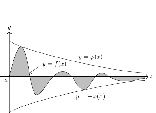
Figure 3. Dominated Integral

Example 2.22.

Primitive functions of $\displaystyle\sin(1/x)$ on $\pm(0,\infty)$ are continuous at $x=\pm 0$.

Example 2.23.

The improper integral (called gamma function)

$$\Gamma(s)=\int_{0}^{\infty}t^{s-1}e^{-t}\,dt$$

exists for $s>0$. Use $t^{s-1}e^{-s}\leq(0,1]t^{s-1}+(1,\infty)M_{s}e^{-t/2}$ with $M_{s}=\sup\{t^{s-1}e^{-t/2};t\geq 1\}<\infty$.

Exercise 10.

Relate the Gaussian integral

$$\int_{0}^{\infty}t^{n}e^{-t^{2}}\,dt\quad(n=0,1,2,\cdots)$$

to the gamma function.

Example 2.24.

As a typical example of conditionally convergent integrals, we pick up $\displaystyle\int_{0}^{\infty}\frac{\sin x}{x}\,dx$. Here the integrand is continuous (even analytic) at $x=0$ and the integral is improper only at $x=\infty$. The integral value turns out to be $\pi/2$ as seen later with the help of repeated integrals or complex analysis.

To see the convergence, we use integration by parts to rewrite

$$\int_{0}^{\infty}\frac{\sin x}{x}\,dx=\int_{0}^{\infty}\frac{\sin(2x)}{x}\,dx=\int_{0}^{\infty}\left(\frac{\sin x}{x}\right)^{2}\,dx+\left[\frac{(\sin x)^{2}}{x}\right]_{0}^{\infty},$$

where the last integral is absolutely convergent by Proposition 2.21.

It is not absolutely convergent, however, because

$$\int_{0}^{\infty}\frac{|\sin x|}{x}\,dx =\sum_{n=1}^{\infty}\int_{\pi(n-1)}^{\pi n}\frac{|\sin x|}{x}\,dx$$

$$\geq\sum_{n=1}^{\infty}\frac{1}{\pi n}\int_{\pi(n-1)}^{\pi n}|\sin x|\,dx=\sum_{n=1}^{\infty}\frac{2}{\pi n}=\infty.$$

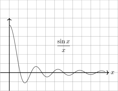
Figure 4. Sinc Function

Exercise 11.

Show that the Fresnel integrals

$$\int_{0}^{\infty}\cos t^{2}\,dt,\quad\int_{0}^{\infty}\sin t^{2}\,dt$$

have meanings as improper integrals. Hint: Change the integral variable to $t=\sqrt{x}$ and then use the same trick as in the above example. We shall later show that their values are $\sqrt{\pi/8}$ by computing a double integral relative to polar coordinates.

Figure 5. Fresnel Integral

Here are more amusing examples of improper integrals.

Example 2.25.

$\displaystyle\int_{0}^{\infty}\frac{\sin^{3}x}{x^{2}}\,dx=\frac{3}{4}\log 3$.

This improper integral is absolutely convergent and the expression

$$\frac{1}{4}\int_{0}^{\infty}\frac{3\sin x-\sin(3x)}{x^{2}}\,dx$$

allows us to apply the Frullani integral for $f(t)=(\sin t)/t$ with $a=1$ and $b=3$ to get the value.

Example 2.26 (Euler).

$I=\displaystyle\int_{0}^{\pi/2}\log(\sin x)\,dx=-\frac{\pi}{2}\log 2$.

First observe that the integral is improper at the boundary $x=0$ but is absolutely convergent.

From the translational invariance $\displaystyle I=\int_{\pi/2}^{\pi}\log(\sin x)\,dx$ and the reflection invariance $I=\displaystyle\int_{0}^{\pi/2}\log(\cos x)\,dx$,

$$I =\frac{1}{2}\int_{0}^{\pi}\log(\sin x)\,dx=\int_{0}^{\pi/2}\log(\sin(2x))\,dx\ (\text{scale is modified by $2$})$$

$$=\int_{0}^{\pi/2}\log 2\,dx+\int_{0}^{\pi/2}\log(\sin x)\,dx+\int_{0}^{\pi/2}\log(\cos x)\,dx$$

$$=\frac{\pi}{2}\log 2+2I.$$

Exercise 12.

With the help of $\sin x\geq 2x/\pi$ ($0\leq x\leq\pi/2$) show the absolute convergence of $\int_{0}^{\pi/2}\log(\sin x)\,dx$.

Theorem 2.27 (Continuity in Laplace Transform).

Let $f:(0,\infty)\to\text{\ym R}$ be an improperly integrable function which is continuous on $(0,a]\sqcup[b,\infty)$ for some $0<a<b<\infty$. Then $e^{-rt}f(t)$ ($r>0$) is an improperly integrable function of $t>0$ and the Laplace transform $\displaystyle\int_{0}^{\infty}e^{-rt}f(t)\,dt$ of $f$ is a continuous function of $r>0$ satisfying

$$\lim_{r\to+0}\int_{0}^{\infty}e^{-rt}f(t)\,dt=\int_{0}^{\infty}f(t)\,dt.$$

Proof.

We first consider the case that $f$ is continous on $(0,\infty)$. Let $\displaystyle F(x)=-\int_{x}^{\infty}f(t)\,dt$ ($x>0$) be a primitive function of $f$ satisfying $\displaystyle\lim_{x\to\infty}F(x)=0$ and $\displaystyle\lim_{x\to+0}F(x)=-\int_{0}^{\infty}f(t)\,dt$ at boundaries. Then $(F(t)e^{-rt})^{\prime}=f(t)e^{-rt}-rF(t)e^{-rt}$, which is integrated to get

$$\int_{x}^{y}e^{-rt}f(t)\,dt=e^{-rx}\int_{x}^{\infty}f(t)\,dt-e^{-ry}\int_{y}^{\infty}f(t)\,dt+r\int_{x}^{y}e^{-rt}F(t)\,dt.$$

Since the last integrand is absolutely integrable on $(0,\infty)$ by Proposition 2.21, we can take the limit $x\to+0$, $y\to\infty$ to have

$$\int_{0}^{\infty}e^{-rt}f(t)\,dt-\int_{0}^{\infty}f(t)\,dt=r\int_{0}^{\infty}e^{-rt}F(t)\,dt.$$

To see the parametric behavior of the right hand side as $r\to+0$, we split the integral domain at some $R>0$ and estimate partial terms by

$$r\int_{0}^{R}e^{-rt}|F(t)|\,dt \leq rR\sup_{t>0}|F(t)|,$$

$$r\int_{R}^{\infty}e^{-rt}|F(t)|\,dt \leq e^{-rR}\sup_{t\geq R}|F(t)|\leq\sup_{t\geq R}|F(t)|.$$

We first take $R$ large enough so that the second term is small and then choose $r>0$ small enough so that $rR$ is small. In total, the right hand side turns out to converge to $0$ as $r\to+0$.

For the parametric continuity, we show that $\displaystyle\int_{0}^{\infty}e^{-rt}F(t)\,dt$ is continuous in $r>0$. To see this, let $r,s\geq\delta>0$ and estimate an absolutely convergent integral $\displaystyle\int_{0}^{\infty}(e^{-rt}-e^{-st})F(t)\,dt$ by

$$\int_{0}^{\infty}|e^{-rt}-e^{-st}||F(t)|\,dt \leq\sup_{x>0}|F(x)|\int_{0}^{\infty}|e^{-rt}-e^{-st}|\,dt$$

$$\leq\sup_{x>0}|F(x)|\int_{0}^{\infty}dt\,\left|\int_{r}^{s}te^{-ut}\,du\right|$$

$$\leq\sup_{x>0}|F(x)|\int_{0}^{\infty}dt\,te^{-\delta t}|r-s|$$

$$=\sup_{x>0}|F(x)|\frac{|r-s|}{\delta^{2}}.$$

Now we relax $f$ to be continuous on $(0,a]\sqcup[b,\infty)$. By replacing $[a,b]f$ with a continuous function on $[a,b]$, we can write $f=g+h$ with $g$ an improperly integrable continuous function on $(0,\infty)$ and $(a,b)h=h\in S_{\uparrow}(\text{\ym R})\cap S_{\downarrow}(\text{\ym R})$ (cf. Corollary 2.7).

Since $e^{-rt}h(t)$ belongs to $S_{\uparrow}\cap S_{\downarrow}$ as a product of $(a,b)e^{-rt}\in S_{\uparrow}\cap S_{\downarrow}$ and $h$ (Proposition 2.5 (iii)), the problem is reduced to showing that $\int_{a}^{b}e^{-rt}h(t)\,dt$ is continuous in $r\geq 0$, which is checked by repeating the parametric continuity in the wholly continuous case, this time by using the boundedness of $h$. ∎

Cauchy-Riemann-Darboux Approach Originally integral was invented as a limit-sum of infinitesimals, which was necessary and useful in mathematical modelling of differential objects. We shall here describe our definite integrals according to historical developments due to Cauchy, Riemann and Darboux. Instead of somewhat mysterious notion of infinitesimals, we work with partitioning of an interval and make the size of interval parts smaller and smaller.

Consider a continuous function $f$ defined on a bounded closed interval $[a,b]$ and regard it as a function on ℝ by zero-extension.

For a partition $\Delta=\{a=x_{0}<x_{1}<\dots<x_{m}=b\}$ of $[a,b]$ and a choice $\xi=(\xi_{i})$ of sample points $\xi_{i}$ from subintervals $(x_{i-1},x_{i}]$, let

$$f^{\Delta}=\sum_{i=1}^{m}(x_{i-1},x_{i}]\sup f((x_{i-1},x_{i}]),\quad f_{\Delta}=\sum_{i=1}^{m}(x_{i-1},x_{i}]\inf f((x_{i-1},x_{i}])$$

and

$$f_{\Delta,\xi}=\sum_{i=1}^{m}(x_{i-1},x_{i}]f(\xi_{i})$$

so that $f_{\Delta}\leq(a,b]f\leq f^{\Delta}$ and $f_{\Delta}\leq f_{\Delta,\xi}\leq f^{\Delta}$.

Note that $f\mapsto f_{\Delta,\xi}$ is linear in $f$, whereas not for $f_{\Delta}$ and $f^{\Delta}$, but these behave simply under a finer partition $\Delta^{\prime}\supset\Delta$; $f_{\Delta}\leq f_{\Delta^{\prime}}\leq f^{\Delta^{\prime}}\leq f^{\Delta}$.

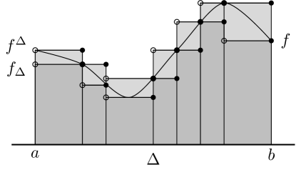
Figure 6. Darboux Approximation

Let $|\Delta|=\max\{x_{1}-x_{0},\dots,x_{m}-x_{m-1}\}$ be the mesh size of $\Delta$. By uniform continuity of $f$ on $[a,b]$,

$$C_{f}(\delta)=\sup\{|f(s)-f(t)|;|s-t|\leq\delta\}$$

descreases to $0$ as $\delta\downarrow 0$ (Theorem A.3). On the other hand,

$$f^{\Delta}(x)-f_{\Delta}(x)=\sup\{|f(s)-f(t)|;s,t\in(x_{i-1},x_{i}]\}$$

for $x\in(x_{i-1},x_{i}]$ shows that $0\leq f^{\Delta}-f_{\Delta}\leq(a,b]C_{f}(|\Delta|)$, which is combined with

$$|f^{\Delta}-f_{\Delta,\xi}|+|f_{\Delta,\xi}-f_{\Delta}|=f^{\Delta}-f_{\Delta}=|f^{\Delta}-(a,b]f|+|(a,b]f-f_{\Delta}|$$

to see that

$$|f_{\Delta,\xi}-(a,b]f|\leq|f^{\Delta}-f_{\Delta,\xi}|+|f^{\Delta}-(a,b]f|\leq 2(f^{\Delta}-f_{\Delta})\leq(a,b](2C_{f}(|\Delta|)).$$

Consequently, for an increasing sequence $\Delta_{1}\subset\Delta_{2}\subset\cdots$ of partitions satisfying $|\Delta_{n}|\to 0$ ($n\to\infty$), we see that $f_{\Delta_{n}}\uparrow(a,b]f$ and $f^{\Delta_{n}}\downarrow(a,b]f$, whence $f=[a,a]f(a)+(a,b]f\in S_{\uparrow}(\text{\ym R})\cap S_{\downarrow}(\text{\ym R})$.

Owing to the linearity of $f_{\Delta,\xi}$ on $f$, we define a positive linear functional of $f\in C([a,b])\subset S_{\uparrow}(\text{\ym R})\cap S_{\downarrow}(\text{\ym R})$ by

$$I_{\Delta,\xi}(f)=I(f_{\Delta,\xi})=\sum_{i}f(\xi_{i})(x_{i}-x_{i-1}),$$

which satisfies

$$\left|I_{\Delta,\xi}(f)-\int_{a}^{b}f(x)\,dx\right| =\Bigl{|}I_{\updownarrow}(f_{\Delta,\xi}-(a,b]f)\Bigr{|}\leq I_{\updownarrow}(|f_{\Delta,\xi}-(a,b]f|)$$

$$\leq I_{\updownarrow}((a,b](2C_{f}(|\Delta|))=2(b-a)C_{f}(|\Delta|).$$

The discussion so far is now summarized as follows:

Theorem 2.28.

Let $[a,b]$ be a bounded closed interval. Then $C([a,b])\subset S_{\uparrow}\cap S_{\downarrow}$ and, for $f\in C([a,b])$, $\lim_{|\Delta|\to 0}\|f_{\Delta,\xi}-f\|_{(a,b]}=0$ and

$$\int_{a}^{b}f(x)\,dx=\lim_{|\Delta|\to 0}I_{\Delta,\xi}(f),$$

i.e., given $\epsilon>0$, we can find $\delta>0$ so that $|\Delta|\leq\delta$ implies $\|f_{\Delta,\xi}-f\|_{(a,b]}\leq\epsilon$ and

$$\left|\int_{a}^{b}f(x)\,dx-I_{\Delta,\xi}(f)\right|\leq\epsilon$$

for any choice $\xi$ of sample points in $\Delta$.

3. Multiple and Repeated Integrals

We now develop multi-dimensional integrals as analogues of the single-variable case: A rectangle is a product set in $\text{\ym R}^{d}$ of bounded intervals such as $[a,b]=[a_{1},b_{1}]\times\dots\times[a_{d},b_{d}]$, $(a,b]=(a_{1},b_{1}]\times\dots\times(a_{d},b_{d}]$ and so on. Note that there are $4^{d}$ choices of end points.

A step function on $\text{\ym R}^{d}$ is defined to be a linear combination of rectangles and the set $S(\text{\ym R}^{d})$ of step functions on $\text{\ym R}^{d}$ is an algebra-lattice.

As in the one-dimensional case, we write $L_{\updownarrow}=S_{\updownarrow}(\text{\ym R}^{d})$ for $L=S(\text{\ym R}^{d})$, which are semilinear lattices and satisfy the following properties.

Proposition 3.1.

1. For $f\in S_{\updownarrow}(\text{\ym R}^{d})$, $0\wedge(\pm f)$ is doubly bounded (i.e., bounded and of bounded support). Consequently functions in $S_{\uparrow}(\text{\ym R}^{d})\cap S_{\downarrow}(\text{\ym R}^{d})$ are doubly bounded as well.

2. A function $f:\text{\ym R}^{d}\to\pm[0,\infty)$ supported by an open rectangle $(a,b)$ of $\text{\ym R}^{d}$ belongs to $S_{\updownarrow}(\text{\ym R}^{d})$ if $f$ is continuous on $(a,b)$.

Corollary 3.2.

Rectangular cuts of $C_{c}(\text{\ym R}^{d})$ are included in $S_{\uparrow}\cap S_{\downarrow}$. Here $C_{c}(\text{\ym R}^{d})$ denotes the set of continuous functions on $\text{\ym R}^{d}$ having bounded supports. In particular the set $C([a,b])$ of continuous functions, which is naturally identified with $[a,b]C_{c}(\text{\ym R}^{d})$ by zero extension to $\text{\ym R}^{d}$, is included in $S_{\uparrow}\cap S_{\downarrow}$.

Proof.

For $f\in C_{c}(\text{\ym R}^{d})$, choose an open rectangle $R$ so that $[f]\subset R$. Then $0\leq R\|f\|\pm f\in S_{\uparrow}$ because it is supoorted by $R$ and continuous on $R$. Thus $f\pm R\|f\|_{\infty}\in S_{\updownarrow}$ and hence $f\in S_{\uparrow}\cap S_{\downarrow}$ in view of $\mp R\|f\|_{\infty}\in S$.

Since $S_{\uparrow}\cap S_{\downarrow}$ is an algebra and contains rectangles, rectangular cuts of $f$ belong to $S_{\uparrow}\cap S_{\downarrow}$. ∎

Exercise 13.

Prove the assertions in Proposition 3.1 (cf. the Cauchy-Riemann-Darboux approach in $\text{\ym R}^{d}$ discussed below).

Given a rectangle $R$, its volume $|R|$ is the product of relevant widths; $|(a,b]|=(b_{1}-a_{1})\cdots(b_{d}-a_{d})$ for example. The volume function is then linearly extended to a positive functional $I$ of $S(\text{\ym R}^{d})$ (called the volume integral), which is also denoted by $I(f)=\int f(x)\,dx$ or simply $\int f$ to suppress integral variables.

The value $I(f)$ is also referred to as the multiple integral of $f$ based on the fact that the following repeated integral formula holds.

$$\int f(x)\,dx=\int\cdots\int f(x_{1},\dots,x_{d})dx_{1}\cdots dx_{d}.$$

Here the order of repetitions of single-variable integrals is irrelevant, i.e., the multiple integral is invariant under permutations of variables because the volume function is invariant under permutations.

Algebraically $S(\text{\ym R}^{d})$ is identified with $S(\text{\ym R})\otimes\dots\otimes S(\text{\ym R})$ and the volume integral $I_{d}$ on $S(\text{\ym R}^{d})$ is nothing but the tensor product $I_{1}^{\otimes d}=I_{1}\otimes\dots\otimes I_{1}$ of the width integral $I_{1}$ on $S(\text{\ym R})$. Thus, if we denote by $I^{(j)}:S(\text{\ym R}^{d})\to S(\text{\ym R}^{d-1})$ the partial width integral $1\otimes\dots\otimes I_{1}\otimes 1\otimes\dots\otimes 1$ on the $j$-th variable, then $I_{d}$ is realized as repetitions of $I^{(j)}$ by $d$-times.

Multiple integrals are then continuous relative to monotone convergence because each partial integral $I^{(j)}$ is continuous (or one can repeat the one-dimensional argument based on a reassembling lemma for countably many rectangles).

The volume integral $I$ on $S(\text{\ym R}^{d})$ is thus a preintegral and we can talk about its extension $I_{\updownarrow}$ to $S_{\updownarrow}(\text{\ym R}^{d})$, which are permutation-invariant and also denoted by $I_{\updownarrow}(f)=\int f(x)\,dx\in\pm(-\infty,\infty]$ for $f\in S_{\updownarrow}(\text{\ym R}^{d})$ as in the case $d=1$.

We can even apply the same argument in the monotone extension of $I$ to see that each partial integral $I^{(j)}$ is monotone-continuously extended to $S_{\updownarrow}(\text{\ym R}^{d})\to S_{\updownarrow}(\text{\ym R}^{d-1})$ and obtain the following.

Proposition 3.3.

The repeated integral formula is valid even for $f\in S_{\updownarrow}(\text{\ym R}^{d})$, where each single-variable integral is realized by $I_{\updownarrow}$ on $S_{\updownarrow}(\text{\ym R})$.

Notice that, as in the width integral, values on rectangles of lower dimensions are irrelevant in volume integrals and a systematic use of open-closed rectangles enables us to simplify describing approximation process in integrals as seen below.

For (bounded) continuous functions of bounded support, we can describe the integral also by the Cauchy-Riemann-Darboux approach. Given a closed rectangle $[a,b]$ and a multiple partition $\Delta=\Delta_{1}\times\dots\times\Delta_{d}$ of $[a,b]$, the rectangle $(a,b]$ is then expressed by a disjoint union of open-closed rectangles of the form $R=R_{1}\times\dots\times R_{d}$ with $R_{j}$ an open-closed interval part in $\Delta_{j}$.

Associated with a bounded function $f:(a,b]\to\text{\ym R}$, introduce step functions on $\text{\ym R}^{d}$ by

$$f^{\Delta}=\sum_{R}R\,(\sup f(R)),\quad f_{\Delta}=\sum_{R}R\,(\inf f(R))$$

and, given a family $\xi=(\xi_{R}\in R)$ of sample points in the decomposition $(a,b]=\bigsqcup R$, let

$$f_{\Delta,\xi}=\sum_{R}Rf(\xi_{R})\in S(\text{\ym R}^{d})$$

and define a positive linear functional of $f\in C([a,b])$ by

$$I_{\Delta,\xi}(f)=I(f_{\Delta,\xi})=\sum_{R}Rf(\xi_{R})$$

in such a way that $f_{\Delta}\leq f\leq f^{\Delta}$ and $f_{\Delta}\leq f_{\Delta,\xi}\leq f^{\Delta}$.

If $\Delta^{\prime}=\Delta_{1}^{\prime}\times\dots\times\Delta_{d}^{\prime}$ is a refinement of $\Delta$ in the sense that $\Delta_{j}\subset\Delta_{j}^{\prime}$ ($1\leq j\leq d$), then $f_{\Delta}\leq f_{\Delta^{\prime}}\leq f^{\Delta^{\prime}}\leq f^{\Delta}$.

The mesh size of $\Delta$ is by definition $|\Delta|=|\Delta_{1}|\vee\dots\vee|\Delta_{d}|$.

Example 3.4.

Let $\Delta^{(l)}$ ($l\geq 1$) be the $l$-th dyadic partition of $[a,b]$. Then $\Delta^{(l)}$ is increasing in $l$ and $|\Delta^{(l)}|=2^{-l}\max\{b_{j}-a_{j};1\leq j\leq d\}$.

Theorem 3.5.

Let $f\in C([a,b])\subset S_{\uparrow}(\text{\ym R}^{d})\cap S_{\downarrow}(\text{\ym R}^{d})$ with $[a,b]$ a closed rectangle in $\text{\ym R}^{d}$. Then $\displaystyle\lim_{|\Delta|\to 0}\|f_{\Delta,\xi}-f\|_{(a,b]}=0$ and

$$\int_{[a,b]}f(x)\,dx=\lim_{|\Delta|\to 0}I_{\Delta,\xi}(f),$$

i.e., given $\epsilon>0$, we can find $\delta>0$ so that $|\Delta|\leq\delta$ implies $\|f_{\Delta,\xi}-f\|_{(a,b]}\leq\epsilon$ and $|I_{\Delta,\xi}(f)-\int_{[a,b]}f|\leq\epsilon$ for any choice $\xi$ of sample points.

Moreover, each partial integral $I^{(j)}$ ($1\leq j\leq d$) gives rise to a linear map $C([a,b])\to C([a,b]_{j})$, where

$$[a,b]_{j}=[a_{1},b_{1}]\times\dots[a_{j-1},b_{j-1}]\times[a_{j+1},b_{j+1}]\times\dots\times[a_{d},b_{d}],$$

so that each single-variable integral in the repeated integral formula of $\int_{[a,b]}f(x)\,dx$ in Proposition 3.3 is described as a width integral on $C([a_{j},b_{j}])\subset S_{\uparrow}(\text{\ym R})\cap S_{\downarrow}(\text{\ym R})$.

Exercise 14.

Check the above theorem with the help of uniform continuity (Theorem A.3).

Exercise 15.

Given a vector-valued function $F=(F_{1},\dots,F_{l}):[a,b]\to\text{\ym R}^{l}$ with $F_{j}\in C([a,b])$, show that

$$\int_{[a,b]}F(x)\,dx\equiv\Bigl{(}\int_{[a,b]}F_{j}(x)\,dx\Bigr{)}_{1\leq j\leq l}\in\text{\ym R}^{l}.$$

satisfies

$$\left|\int_{[a,b]}F(x)\,dx\right|\leq\int_{[a,b]}|F(x)|\,dx,$$

where $|v|=\sqrt{(v_{1})^{2}+\dots+(v_{l})^{2}}$ for $v=(v_{1},\dots,v_{l})\in\text{\ym R}^{l}$.

Example 3.6.

Let $r>0$ and consider $f(x,y)=(x+y)^{-r}$ supported by $[x>a,y>b]$ ($a\geq 0,b\geq 0$), which belongs to $S_{\uparrow}(\text{\ym R}^{2})$ and $I_{\uparrow}(f)$ is calculated by the repeated integral formula in the following manner:

$$\int_{a}^{\infty}dx\,\int_{b}^{\infty}dy\,(x+y)^{-r} =\int_{a}^{\infty}\frac{1}{r-1}(x+b)^{1-r}\,dx$$

$$=\begin{cases}\frac{1}{(r-1)(r-2)}(a+b)^{2-r}&(r>2),\\ \infty&(r\leq 2).\end{cases}$$

As a supplement to the above theorem, notice that, for functions in $S_{\uparrow}(\text{\ym R}^{d})\cap S_{\downarrow}(\text{\ym R}^{d})$ (which contains $C_{c}(\text{\ym R}^{d})$), each single-variable integral in the repeated integral formula is realized as the width integral on $S_{\uparrow}(\text{\ym R})\cap S_{\downarrow}(\text{\ym R})$.

In the multi-dimensional case, however, it still entails a rectangular character and does not allow all reasonable domains as elements in $S_{\uparrow}\cap S_{\downarrow}$: If $D$ is a bounded open set with its boundary $\partial D$ having a lower-dimensional but non-rectangular shape, then $D\in S_{\uparrow}$ but $D\not\in S_{\downarrow}$. For example, an open disk $D=\{(x,y);x^{2}+y^{2}<1\}$ in $\text{\ym R}^{2}$ belongs to $S_{\uparrow}(\text{\ym R}^{2})$, whereas $D\not\in S_{\downarrow}(\text{\ym R}^{2})$.

This kind of defects come from the fact that $S_{\updownarrow}(\text{\ym R}^{d})$ excludes lower-dimensional subsets other than rectangular ones (as indicators).

Exercise 16.

Show that any open disk $D\not=\emptyset$ does not belong to $S_{\downarrow}(\text{\ym R}^{2})$ as an indicator.

We therefore relax exact-limit description of functions in $L_{\updownarrow}$ to allow exceptional sets such as lower-dimensional boundaries. This is based on the following sophisticated form of the method of exhaustion due to P.J. Daniell. Let $(L,I)$ be an integral system on a set $X$.

Definition 3.7.

Given a function $f:X\to[-\infty,\infty]$, its upper and lower integrals are defined by

$${\overline{I}}(f)=\inf\{I_{\uparrow}(g);g\in L_{\uparrow},f\leq g\},\quad{\underline{I}}(f)=\sup\{I_{\downarrow}(g);g\in L_{\downarrow},g\leq f\},$$

which are elements in the extended real line $\overline{\text{\ym R}}=[-\infty,\infty]$. Recall that $\inf(\emptyset)=\infty$ and $\sup(\emptyset)=-\infty$.

Proposition 3.8.

Let $f,g:X\to[-\infty,\infty]$.

1. ${\underline{I}}(f)=-{\overline{I}}(-f)$.

2. ${\overline{I}}(rf)=r{\overline{I}}(f)$ for $0<r<\infty$.

3. If $f\leq g$, ${\underline{I}}(g)\leq{\underline{I}}(f)\leq{\overline{I}}(f)\leq{\overline{I}}(g)$.

4. When $f+g$ is well-defined, i.e., there is no $x\in X$ satisfying $f(x)=\pm\infty$ and $g(x)=\mp\infty$, we have ${\overline{I}}(f+g)\leq{\overline{I}}(f)+{\overline{I}}(g)$.

5. For $f\in L_{\uparrow}\cup L_{\downarrow}$, we have ${\underline{I}}(f)={\overline{I}}(f)$. Moreover this value is equal to $I_{\uparrow}(f)$ or $I_{\downarrow}(f)$ according to $f\in L_{\uparrow}$ or $f\in L_{\downarrow}$.

Proof.

The assertions (i)–(iv) are immediate from the definition.

To see (v), first notice that ${\overline{I}}(f)=I_{\uparrow}(f)$ ($f\in L_{\uparrow}$) and ${\underline{I}}(f)=I_{\downarrow}(f)$ ($f\in L_{\downarrow}$). Especially, ${\underline{I}}(f)=\overline{I}(f)=I(f)$ for $f\in L$.

Now let $f\in L_{\uparrow}$ and choose $f_{n}\in L$ so that $f_{n}\uparrow f$. Then

$$I_{\uparrow}(f)=\lim_{n}I(f_{n})=\lim_{n}{\underline{I}}(f_{n})\leq{\underline{I}}(f).$$

On the other hand, for $f\in L_{\uparrow}$, we have ${\overline{I}}(f)=I_{\uparrow}(f)$ as already checked. Thus ${\overline{I}}(f)={\underline{I}}(f)$. ∎

Exercise 17.

Supply the details for (i)–(iv).

Since any integral of $f$ should be between $\underline{I}(f)$ and $\overline{I}(f)$, we arrive at the following.

Definition 3.9.

We say that a function $f:X\to\text{\ym R}$ is $I$-integrable or simply integrable if ${\underline{I}}(f)={\overline{I}}(f)\in\text{\ym R}$ (the upper and the lower integrals are finite and coincide). The totality of integrable functions is denoted by $L^{1}(I)$ or simply $L^{1}$. For $f\in L^{1}$, the value ${\underline{I}}(f)={\overline{I}}(f)\in\text{\ym R}$ is denoted by $I^{1}(f)$.

A subset $A$ of $X$ is said to be integrable if it is integrable as an indicator function with its integral $I^{1}(A)$ called the $I$-measure of $A$ and denoted by $|A|_{I}$.

In the case $L=S(\text{\ym R}^{d})$ with the volume integral $I$, $L^{1}$ is denoted by $L^{1}(\text{\ym R}^{d})$ and $I$-integrability is also referred to as being Lebesgue integrable) by a historical reason. In accordance with this, the volume-measure of a Lebesgue integrable set $A$ is called the Lebesgue measure and denoted by $|A|$.

Exercise 18.

For $f:X\to[-\infty,\infty]$ and $g\in L^{1}$, we have $\overline{I}(f+g)=\overline{I}(f)+I^{1}(g)$ and $\underline{I}(f+g)=\underline{I}(f)+I^{1}(g)$.

It is not clear at this point but all reasonable bounded sets turn out to be integrable based on convergence theorems (see Corollary 4.13).

Lemma 3.10.

A function $f:X\to\text{\ym R}$ is integrable if and only if

$$\forall\epsilon>0,\ \exists f_{+}\in L_{\uparrow},\ \exists f_{-}\in L_{\downarrow},\quad f_{-}\leq f\leq f_{+},\ I_{\uparrow}(f_{+})-I_{\downarrow}(f_{-})\leq\epsilon.$$

Moreover, if $f_{-}$ increases ($f_{+}$ decreases) in such a way that $f_{-}\leq f\leq f_{+}$ and $I_{\uparrow}(f_{+})-I_{\downarrow}(f_{-})=I_{\uparrow}(f_{+}-f_{-})\geq 0$ goes to $0$, then

$$I_{\downarrow}(f_{-})\uparrow I(f),\quad I_{\uparrow}(f_{+})\downarrow I(f).$$

Proof.

Use the inequality $I_{\downarrow}(f_{-})\leq{\underline{I}}(f)\leq{\overline{I}}(f)\leq I_{\uparrow}(f_{+})$. ∎

Theorem 3.11.

1. The set $L^{1}$ is a vector lattice on $X$ and includes $L_{\uparrow}\cap L_{\downarrow}$.

2. $I^{1}:L^{1}\to\text{\ym R}$ is a positive linear functional satisfying $I^{1}(f)=I_{\uparrow}(f)=I_{\downarrow}(f)$ for $f\in L_{\uparrow}\cap L_{\downarrow}$. In particular, $I^{1}$ is an extension (called the Daniell extension) of the preintegral $I:L\to\text{\ym R}$.

Proof.

Let $f,g\in L^{1}$. Assume that $f_{+},g_{+}\in L_{\uparrow}$ and $f_{-},g_{-}\in L_{\downarrow}$ satisfy $f_{-}\leq f\leq f_{+}$, $g_{-}\leq g\leq g_{+}$. Then $f_{-}+g_{-}\leq f+g\leq f_{+}+g_{+}$ and we see that

$$I_{\uparrow}(f_{+}+g_{+})-I_{\downarrow}(f_{-}+g_{-})=(I_{\uparrow}(f_{+})-I_{\downarrow}(f_{-}))+(I_{\uparrow}(g_{+})-I_{\downarrow}(g_{-}))$$

can be chosen arbitrarily small, i.e., $f+g\in L^{1}$ and $I(f+g)=I(f)+I(g)$.

Next, let $r>0$. Since $rf_{-}\leq rf\leq rf_{+}$, we see that

$$I_{\uparrow}(rf_{+})-I_{\downarrow}(rf_{-})=r(I_{\uparrow}(f_{+})-I_{\downarrow}(f_{-}))$$

can be arbitrarily small, i.e., $rf\in L^{1}$ and $I(rf)=rI(f)$.

If we notice $-f_{+}\leq-f\leq-f_{-}$ ($-f_{+}\in L_{\downarrow}$, $-f_{-}\in L_{\uparrow}$),

$$I_{\uparrow}(-f_{-})-I_{\downarrow}(-f_{+})=I_{\uparrow}(f_{+})-I_{\downarrow}(f_{-})$$

can be chosen small as well, i.e., $-f\in L^{1}$ and $I(-f)=-I(f)$.

So far we have checked that $L^{1}$ is a vector space and $I$ is a linear functional on $L^{1}$.

To show that $L^{1}$ is closed under the lattice operation, it suffices to check $f\in L^{1}\Longrightarrow f\vee 0\in L^{1}$, which can be seen as follows. From $f_{-}\vee 0\leq f\vee 0\leq f_{+}\vee 0$, we have the inequality

$$0\leq f_{+}\vee 0-f_{-}\vee 0\leq f_{+}-f_{-},$$

which is used to see that

$$0\leq I_{\uparrow}(f_{+}\vee 0)-I_{\downarrow}(f_{-}\vee 0)=I_{\uparrow}(f_{+}\vee 0-f_{-}\vee 0)\leq I_{\uparrow}(f_{+}-f_{-})$$

can be chosen arbitrarily small. In particular, for $f\geq 0$, $I(f)=I(f\vee 0)\geq 0$ as a limit of $I_{\uparrow}(f_{+}\vee 0)\geq 0$.

Finally, if $f\in L_{\uparrow}\cap L_{\downarrow}$ , we can find $f_{\pm}\in L$ such that $f_{-}\leq f\leq f_{+}$, which, together with Proposition3.8 (vi), shows that ${\underline{I}}(f)={\overline{I}}(f)\in[I(f_{-}),I(f_{+})]$ is finite. ∎

Definition 3.12.

The Daniell extension of the volume integral on $S(\text{\ym R}^{d})$ is called Lebesgue integral.

Example 3.13.

Target functions of definite integral are Lebesgue integrable with definite integrals equal to Lebesgue integrals. For improper integrals, conditionally convergent ones are not Lebesgue integrable because $L^{1}(\text{\ym R})$ is closed under taking absolute value functions.

We shall see in the next section that absolutely convergent ones are Lebesgue integrable.

Exercise 19.

Show that integrable sets are closed under taking finite unions and differences.

For a later use, we record here the following.

Proposition 3.14.

1. A function $f$ in $L_{\updownarrow}$ is integrable if and only if it is real-valued and $\pm I_{\updownarrow}(f)<\infty$.

2. $L^{1}\cap L_{\uparrow}-L^{1}\cap L_{\uparrow}$ is a linear lattice and $I^{1}(f_{\uparrow}+f_{\downarrow})=I_{\uparrow}(f_{\uparrow})+I_{\downarrow}(f_{\downarrow})$ for $f_{\updownarrow}\in L_{\updownarrow}\cap L^{1}$.

3. $L^{1}\cap L_{\uparrow}=L^{1}\cap L_{\uparrow}^{+}+L$ and $L^{1}\cap L_{\uparrow}-L^{1}\cap L_{\uparrow}=L^{1}\cap L_{\uparrow}^{+}-L^{1}\cap L_{\uparrow}^{+}$.

Proof.

(i) If $f\in L_{\uparrow}$ is integrable, there is $h\in L_{\uparrow}$ such that $f\leq h$ and $I_{\uparrow}(h)<\infty$, whence $I_{\uparrow}(f)<\infty$.

Conversely, if $f\in L_{\uparrow}$ is real-valued, there exists an increasing sequence $(f_{n})$ in $L$ satisfying $f_{n}\uparrow f$ and $I(f_{n})\leq\underline{I}(f)\leq\overline{I}(f)\leq I_{\uparrow}(f)$ for $n\geq 1$ shows that $\underline{I}(f)=\overline{I}(f)=I_{\uparrow}(f)$. Thus, if the condition $I_{\uparrow}(f)<\infty$ is further satisfied, $f$ is integrable and $I^{1}(f)=I_{\uparrow}(f)$.

(ii) Since $L_{\uparrow}$ is semilinear and $L^{1}$ is a linear space, $L^{1}\cap L_{\uparrow}-L^{1}\cap L_{\uparrow}$ is a linear space. Let $f=f_{1}-f_{2}$ with $f_{j}\in L^{1}\cap L_{\uparrow}$. Since both $L^{1}$ and $L_{\uparrow}$ are lattices, $f_{1}\diamond f_{2}\in L^{1}\cap L_{\uparrow}$ and then $|f|=f_{1}\vee f_{2}-f_{1}\wedge f_{2}\in L^{1}\cap L_{\uparrow}-L^{1}\cap L_{\uparrow}$. Thus $L^{1}\cap L_{\uparrow}-L^{1}\cap L_{\uparrow}$ is closed under taking absolute values.

(iii) Let $f\in L_{\uparrow}$ be expressed as $f_{n}\uparrow f$ with $f_{n}\in L$. If $f\in L^{1}$, $f-f_{1}\in L^{1}\cap L_{\uparrow}^{+}$ and $f=(f-f_{1})+f_{1}\in L^{1}\cap L_{\uparrow}^{+}+L$. By a similar expression for another $g\in L^{1}\cap L_{\uparrow}$, we see that

$$f-g =(f-f_{1})-(g-g_{1})+f_{1}-g_{1}$$

$$=(f-f_{1})-(g-g_{1})+0\vee(f_{1}-g_{1})-0\vee(g_{1}-f_{1})$$

$$=\bigl{(}f-f_{1}+0\vee(f_{1}-g_{1})\bigr{)}-\bigl{(}g-g_{1}+0\vee(g_{1}-f_{1})\bigr{)}$$

with $f-f_{1}+0\vee(f_{1}-g_{1})$ and $g-g_{1}+0\vee(g_{1}-f_{1})$ in $L^{1}\cap L_{\uparrow}^{+}$. ∎

4. Convergence Theorems

We now establish a series of convergence theorems on integrable functions, which exhibits some completeness (or maximality) of Daniell extensions. To this end, we need to look into $I_{\updownarrow}$ more closely.

Lemma 4.1.

1. $f_{n}\uparrow f$ with $f_{n}\in L_{\uparrow}$ implies $f\in L_{\uparrow}$ and $I_{\uparrow}(f_{n})\uparrow I_{\uparrow}(f)$.

2. $f_{n}\downarrow f$ with $f_{n}\in L_{\downarrow}$ implies $f\in L_{\downarrow}$ and $I_{\downarrow}(f_{n})\downarrow I_{\downarrow}(f)$.

Proof.

By symmetry it suffices to prove (i). For each $f_{n}\in L_{\uparrow}$, choose a sequence $(f_{n,m})_{m\geq 1}$ so that $f_{n,m}\uparrow f_{n}$. To get the monotonicity for $(f_{n,m})_{n\geq 1}$, we introduce their push-ups by

$$g_{n,m}=f_{1,m}\vee f_{2,m}\vee\dots\vee f_{n,m}.$$

Here $g_{1,m}=f_{1,m}$ by definition. Clearly $g_{n,m}$ is increasing in $n$. Since $f_{n,m}$ is increasing in $m$, so is $g_{n,m}$ in $m$. Moreover

$$f_{n,m}\leq g_{n,m}\leq f_{1}\vee f_{2}\vee\dots\vee f_{n}=f_{n}$$

shows that $g_{n,m}\uparrow f_{n}$ for each $n$.

With this preparation in hand, we pick up the diagonal $(g_{n,n})_{n\geq 1}$, which is an increasing sequence in $L$. Taking the limit $m\to\infty$ in the obvious inequality

$$f_{n,m}\leq g_{n,m}\leq g_{m,m}\leq f_{m},\quad m\geq n,$$

we obtain

$$f_{n}\leq\lim_{m\to\infty}g_{m,m}\leq f$$

and then, letting $n\to\infty$,

$$f=\lim_{m\to\infty}g_{m,m}\in L_{\uparrow}.$$

Now $I_{\uparrow}$ is applied in the above inequalities to obtain

$$I(f_{n,m})\leq I(g_{m,m})\leq I_{\uparrow}(f_{m})\quad(m\geq n)$$

and, after taking the limit $m\to\infty$,

$$I_{\uparrow}(f_{n})\leq I_{\uparrow}(f)\leq\lim_{m\to\infty}I_{\uparrow}(f_{m}).$$

Thus, letting $n\to\infty$, we finally have

$$\lim_{n\to\infty}I_{\uparrow}(f_{n})=I_{\uparrow}(f).$$

∎

Corollary 4.2.

For a sequence $f_{n}\in L_{\uparrow}^{+}$, $\sum_{n}f_{n}\in L_{\uparrow}$ and

$$I_{\uparrow}\left(\sum_{n}f_{n}\right)=\sum_{n}I_{\uparrow}(f_{n}).$$

Proof.

Though it is immediate from (i) in the lemma, this is a core of convergence theorems discussed below, whence we shall provide a direct proof as a record (the double sum identity being the essence of convergence theorems).

We first remark that a function $h:X\to[0,\infty]$ belongs to $L_{\uparrow}^{+}$ if and only if $h=\sum h_{n}$ for a sequence $(h_{n})$ in $L^{+}$. Moreover, if this is the case, we have $I_{\uparrow}(h)=\sum I(h_{n})$.

Returning to the proof, this remark enables us to choose sequences $(h_{m,n})_{m\geq 1}$ in $L^{+}$ so that $f_{n}=\sum_{m}h_{m,n}$ and $I_{\uparrow}(f_{n})=\sum_{m}I(h_{m,n})$. Then $\sum_{n}f_{n}=\sum_{m,n}h_{m,n}\in L_{\uparrow}^{+}$ and

$$I_{\uparrow}\left(\sum_{n}f_{n}\right)=\sum_{m,n}I(h_{m,n})=\sum_{n}\left(\sum_{m}I(h_{m,n})\right)=\sum_{n}I_{\uparrow}(f_{n}).$$

∎

Lemma 4.3 (subadditivity of upper integrals).

If a function $f:X\to[0,\infty]$ has an expression $f=\sum_{n=1}^{\infty}f_{n}$ with $f_{n}\geq 0$, then

$${\overline{I}}(f)\leq\sum_{n=1}^{\infty}{\overline{I}}(f_{n}).$$

Proof.

We may assume that ${\overline{I}}(f_{n})<\infty$ ($n\geq 1$). Given any $\epsilon>0$, if we choose $g_{n}\in L_{\uparrow}^{+}$ so that

$$f_{n}\leq g_{n},\quad I(g_{n})=I_{\uparrow}(g_{n})\leq{\overline{I}}(f_{n})+\frac{\epsilon}{2^{n}}.$$

Then, in view of $\sum_{n}g_{n}\in L_{\uparrow}^{+}$ and $I_{\uparrow}(\sum_{n}g_{n})=\sum_{n}I_{\uparrow}(g_{n})$ (Corollary 4.2), we have

$${\overline{I}}(f)\leq I_{\uparrow}\left(\sum_{n}g_{n}\right)=\sum_{n}I_{\uparrow}(g_{n})\leq\sum_{n}{\overline{I}}(f_{n})+\sum_{n}\frac{\epsilon}{2^{n}}=\sum_{n}{\overline{I}}(f_{n})+\epsilon.$$

∎

Theorem 4.4 (Monotone Convergence Theorem).

For a real-valued function $f$ satisfying $f_{n}\uparrow f$ with $f_{n}\in L^{1}$, $f$ is integrable if and only if $\displaystyle\lim_{n\to\infty}I^{1}(f_{n})<\infty$. Moreover, if this is the case, $\displaystyle I^{1}(f)=\lim_{n\to\infty}I^{1}(f_{n})$.

Proof.

From $I^{1}(f_{n})={\overline{I}}(f_{n})\leq{\overline{I}}(f)$, $\displaystyle\lim_{n\to\infty}I(f_{n})=\infty$ implies ${\overline{I}}(f)=\infty$ and hence $f\not\in L^{1}$. Let $\displaystyle\lim_{n\to\infty}I^{1}(f_{n})<\infty$. We apply the above lemma to $f-f_{1}=\sum_{n=1}^{\infty}(f_{n+1}-f_{n})$ and obtain

$${\overline{I}}(f-f_{1})\leq\sum_{n=1}^{\infty}{\overline{I}}(f_{n+1}-f_{n})=\sum_{n=1}^{\infty}I^{1}(f_{n+1}-f_{n})\\ =\sum_{n=1}^{\infty}\Bigl{(}I^{1}(f_{n+1})-I^{1}(f_{n})\Bigr{)}=\lim_{n\to\infty}I^{1}(f_{n+1})-I^{1}(f_{1}),$$

whence

$${\overline{I}}(f)\leq{\overline{I}}(f_{1})+{\overline{I}}(f-f_{1})=I^{1}(f_{1})+{\overline{I}}(f-f_{1})\leq\lim_{n}I^{1}(f_{n}).$$

On the other hand, if we take a limit in $I^{1}(f_{n})={\underline{I}}(f_{n})\leq{\underline{I}}(f)$,

$$\lim_{n}I^{1}(f_{n})\leq{\underline{I}}(f)\leq{\overline{I}}(f)\leq\lim_{n}I^{1}(f_{n}),$$

showing that $f$ is integrable and $I^{1}(f)=\lim_{n}I^{1}(f_{n})$. ∎

Corollary 4.5.

The positive linear functional $I^{1}$ is continuous, i.e., $I^{1}$ is a preintegral on $L^{1}$.

Exercise 20.

Show that integrable sets are closed under taking countable intersections.

As an illustration of usefulness of the monotone convergence theorem, we shall derive the de Moivre-Stirling formula (known also as Stirling’s formula) of the gamma function:

$$\lim_{x\to\infty}\frac{\Gamma(x+1)}{\sqrt{2\pi x}x^{x}e^{-x}}=1.$$

To see this, in the expression

$$\Gamma(x+1)=\int_{0}^{\infty}s^{x}e^{-s}\,ds,$$

observe that the logarithmic integrand $h(s,x)=\log(s^{x}e^{-s})$ ($s>0$ with $x>0$ a parameter) is maximized at $s=x$ with its Taylor expansion around $s=x$ given by

$$h(s,x)=x\log x-x-\frac{1}{2}\frac{(s-x)^{2}}{x}+\cdots,$$

which suggests us to introduce the new variable $t=(s-x)/\sqrt{x}$ to have

$$\Gamma(x+1)=e^{x}x^{x}\sqrt{x}\int_{-\sqrt{x}}^{\infty}\left(1+\frac{t}{\sqrt{x}}\right)^{x}e^{-t\sqrt{x}}\,dt$$

and the problem is reduced to showing

$$\lim_{x\to\infty}\int_{-\sqrt{x}}^{\infty}\left(1+\frac{t}{\sqrt{x}}\right)^{x}e^{-t\sqrt{x}}\,dt=\sqrt{2\pi}.$$

To see the asymptotic behavior of this integrand, we again consider its logarithm $g(t,x)$ ($t>0,x>0$) and rewrite it as

$$g(t,x) =x\log\left(1+\frac{t}{\sqrt{x}}\right)-t\sqrt{x}$$

$$=x\int_{0}^{t/\sqrt{x}}\frac{1}{1+u}\,du-x\int_{0}^{t/\sqrt{x}}du$$

$$=-x\int_{0}^{t/\sqrt{x}}\frac{u}{1+u}\,du=-\int_{0}^{t}\frac{v}{1+v/\sqrt{x}}\,dv.$$

From the last expression, a continuous function $f$ of $t\in\text{\ym R}$ and $x>0$ defined by

$$f(t,x)=\begin{cases}e^{g(t,x)}&(t>-\sqrt{x}),\\ 0&(t\leq-\sqrt{x})\end{cases}$$

satisfies $f(t,x)\downarrow e^{-t^{2}/2}$ ($t\geq 0$) and $f(t,x)\uparrow e^{-t^{2}/2}$ ($t\leq 0$) for the limit $x\uparrow\infty$. Notice $f(0,x)=1$ ($x>0$).

Since $f(t,x)\leq f(t,1)=(1+t)e^{-t}$ ($x\geq 1$, $t\geq 0$) and $f(t,x)\leq e^{-t^{2}/2}$ ($x>0$, $t\leq 0$) are integrable functions of $t\in\text{\ym R}$, we can apply the monotone convergence theorem to see that

$$\int_{-\sqrt{x}}^{\infty}\left(1+\frac{t}{\sqrt{x}}\right)^{2}e^{-t\sqrt{x}}\,dt=\int_{-\infty}^{\infty}f(t,x)\,dt=\int_{0}^{\infty}f(t,x)\,dt+\int_{-\infty}^{0}f(t,x)\,dt$$

converges to

$$\int_{-\infty}^{\infty}e^{-t^{2}/2}\,dt=\sqrt{2\pi}$$

as $x\to\infty$ (see Example 6.5 for the last equality) and we are done.

Exercise 21.

Check the continuity of $f(t,x)$ in the above proof.

Theorem 4.6 (Dominated Convergence Theorem).

If a sequence $(f_{n})$ in $L^{1}$ and a function $g\in L^{1}$ satisfy $|f_{n}|\leq g$ ($n\geq 1$), then $\inf_{n\geq 1}f_{n}$, $\sup_{n\geq 1}f_{n}$, $\liminf_{n\to\infty}f_{n}$ and $\limsup_{n\to\infty}f_{n}$ are all integrable and

$$I^{1}(\liminf f_{n})\leq\liminf I^{1}(f_{n})\leq\limsup I^{1}(f_{n})\leq I^{1}(\limsup f_{n}).$$

In particular, if the limit function $\displaystyle f=\lim_{n\to\infty}f_{n}$ exists, $f\in L^{1}$ and

$$I^{1}(f)=\lim_{n\to\infty}I^{1}(f_{n}).$$

Proof.

For a natural number $m$, we see

$$-g\leq\inf_{n\geq m}f_{n}\leq f_{m}\wedge\dots\wedge f_{n}\leq f_{m}\vee\dots\vee f_{n}\leq\sup_{n\geq m}f_{n}\leq g$$

and

$$f_{m}\wedge\dots\wedge f_{n}\downarrow\inf_{n\geq m}f_{n},\quad f_{m}\vee\dots\vee f_{n}\uparrow\sup_{n\geq m}f_{n}.$$

whence, by the monotone convergence theorem and the positivity of $I^{1}$, we have $\inf_{n\geq m}f_{n},\sup_{n\geq m}f_{n}\in L^{1}$ and

$$I^{1}(\inf_{n\geq m}f_{n})=\lim_{n}I^{1}(f_{m}\wedge\dots\wedge f_{n})\leq\lim_{n}I^{1}(f_{m})\wedge\dots\wedge I^{1}(f_{n})=\inf_{n\geq m}I^{1}(f_{n})$$

$$I^{1}(\sup_{n\geq m}f_{n})=\lim_{n}I^{1}(f_{m}\vee\dots\vee f_{n})\geq\lim_{n}I^{1}(f_{m})\vee\dots\vee I^{1}(f_{n})=\sup_{n\geq m}I^{1}(f_{n}).$$

In other words, we have

$$-I^{1}(g)\leq I^{1}(\inf_{n\geq m}f_{n})\leq\inf_{n\geq m}I^{1}(f_{n})\leq\sup_{n\geq m}I^{1}(f_{n})\leq I^{1}(\sup_{n\geq m}f_{n})\leq I^{1}(g)$$

and then, again by the monotone convergence theorem, we see that $\liminf_{n}f_{n}$ and $\limsup_{n}f_{n}\in L^{1}$ are integrable and satisfy

$$-I^{1}(g)\leq I^{1}(\liminf_{n}f_{n})\leq\liminf_{n}I^{1}(f_{n})\\ \leq\limsup_{n}I^{1}(f_{n})\leq I^{1}(\limsup_{n}f_{n})\leq I^{1}(g).$$

∎

Since $(L^{1},I^{1})$ is agian an integral system, we can apply the Daniel extension but it does not give a strict extension. Let $L^{1}_{\updownarrow}=(L^{1})_{\updownarrow}$ and $I^{1}_{\updownarrow}:L^{1}_{\updownarrow}\to\pm(-\infty,\infty]$ be the monotone extensions of $(L^{1},I^{1})$ with the associated upper and lower integrals denoted by $\overline{I^{1}}$ and $\underline{I^{1}}$ respectively.

Theorem 4.7 (Maximality of Daniell Extension).

We have $\overline{I^{1}}=\overline{I}$ and $\underline{I^{1}}=\underline{I}$. The Daniell extension of $(L^{1},I^{1})$ is therefore $(L^{1},I^{1})$ itself.

Proof.

By symmetry it suffices to show that $\overline{I^{1}}=\overline{I}$. Since $I^{1}$ is an extension of $I$, $I^{1}_{\uparrow}$ extends $I_{\uparrow}$, whence $\overline{I^{1}}(f)\leq\overline{I}(f)$ and the equality holds trivially when $\overline{I^{1}}(f)=\infty$. So we assume that $\overline{I^{1}}(f)<\infty$.

Given $\epsilon>0$, we can find a sequence $(f_{n})$ in $L^{1}$ such that $f_{n}\geq 0$ for $n\geq 2$, $f\leq\sum_{n\geq 1}f_{n}$ and $\sum_{n\geq 1}I^{1}(f_{n})\leq\overline{I^{1}}(f)+\epsilon$. Since $\overline{I}(f_{n})=I^{1}(f_{n})<\infty$ for any $n\geq 1$, we can choose a sequence $(f_{n,j})_{j\geq 1}$ in $L$ so that $f_{n,j}\geq 0$ for $(n,j)\not=(1,1)$, $f_{n}\leq\sum_{j\geq 1}f_{n,j}$ and $\sum_{j\geq 1}I(f_{n,j})\leq\overline{I}(f_{n})+\epsilon/2^{n}$.

Thus $f\leq\sum_{n,j\geq 1}f_{n,j}$ and

$$\sum_{n,j\geq 1}I(f_{n,j})\leq\sum_{n\geq 1}\overline{I}(f_{n})+\epsilon\leq\overline{I^{1}}(f)+2\epsilon$$

imply $\overline{I}(f)\leq\overline{I^{1}}(f)+2\epsilon$, proving the reverse inequality. ∎

Definition 4.8.

Let $L^{1}_{\uparrow}=(L^{1})_{\uparrow}$ and $I^{1}_{\uparrow}=(I^{1})_{\uparrow}:L^{1}_{\uparrow}\to(-\infty,\infty]$. A subset $A\subset X$ is said to be $\bm{\sigma}$-integrable if it is a union of countably many $I$-integrable sets.

When $I$ is the volume integral on $S(\text{\ym R}^{d})$, $\sigma$-integrable sets are said to be Lebesgue measurable. Clearly rectangles are Lebesgue integrable.

Proposition 4.9.

1. A subset $A\subset X$ is $\sigma$-integrable if and only if it belongs to $L^{1}_{\uparrow}$ as an indicator function.

2. $\sigma$-integrable sets are closed under taking countable unions, countable intersections and differences.

3. The intersection of a $\sigma$-integrable set and an integrable set is integrable.

4. Lebesgue measurable sets are closed under taking complements furthermore.

Proof.

Non-trivial is the if part in (i). To see this, we argue as in Corollary C.2: Let $A\in L^{1}_{\uparrow}$ and write $f_{n}\uparrow A$ with $0\leq f_{n}\in L^{1}$. Then, for $f\in L^{1}$ satisfying $0\leq f\leq A$ and $r>0$, the monotone convergence theorem is applied to $(rf_{n})\wedge f\uparrow r\wedge f\leq f$ and we know $r\wedge f\in L^{1}$.

Then $1\wedge n(f-r\wedge f)=n(\frac{1}{n}\wedge(f-r\wedge f))$ as well as $f-r\wedge f$ is integrable. Moreover, $f(x)>r$ ($f(x)-r\wedge f(x)>0$) implies $1\wedge n(f-r\wedge f)\leq f/r$.

Now the push-up formula $1\wedge n(f-r\wedge f)\uparrow[f>r]$ (Lemma C.1) is combined with the monotone convergence theorem to sees that $[f>r]$ is integrable. In particular, $[f_{n}>r]$ is integrable for each $n\geq 1$ and $[f_{n}>r]\uparrow A$ ($n\to\infty$) for $0<r<1$ shows that $A$ is $\sigma$-integrable. ∎

Exercise 22.

Check other parts in Proposition 4.9.

The $I$-measure on $I$-integrable sets is extended to $\sigma$-integrable sets by $I^{1}_{\uparrow}$: In terms of an expression $A_{n}\uparrow A$ with $A_{n}$ $I$-integrable,

$$|A|_{I}=I^{1}_{\uparrow}(A)=\lim_{n\to\infty}|A_{n}|_{I}\in[0,\infty].$$

Proposition 4.10.

Let $f\in L^{1}(I)$ and $A$ be $\sigma$-integrable with respect to $I$. Then $Af\in L^{1}(I)$.

Proof.

We may assume that $f\geq 0$ and first consider an $I$-integrable $A$. Since simple functions $Ar$ ($r>0$) are $I$-integrable, so are $(Ar)\vee f\in L^{1}(I)$ and the monotone convergence theorem is used to see that

$$Af=\lim_{n\to\infty}\Bigl{(}A\frac{1}{n}\Bigr{)}\vee f\in L^{1}(I).$$

Now let $A$ be $\sigma$-integrable and write $A_{n}\uparrow A$ with $A_{n}$ $I$-integrable. Then $A_{n}f\uparrow Af$ with $A_{n}f\in L^{1}(I)$ and $A_{n}f\leq f$. Again the monotone convergence theorem or the dominated convergence theorem works here to see that $Af\in L^{1}(I)$. ∎

For a Lebesgue measurable set $A\subset\text{\ym R}^{d}$ and a Lebesgue integrable function $f$ on $\text{\ym R}^{d}$, the Lebesgue integral of $Af$ is also denoted by

$$\int_{A}f(x)\,dx.$$

Remark 5.

See Appendix C for an overall account on measurable sets and measurable functions.

We now specialize to the volume integral on the space $S(\text{\ym R}^{d})$ of step functions and realize how big $L^{1}(\text{\ym R}^{d})$ is.

Recall (Proposition 3.14) that, if we denote by $S_{\updownarrow}^{1}(\text{\ym R}^{d})$ the totality of real-valued functions in $S_{\updownarrow}(\text{\ym R}^{d})$, say $f_{\updownarrow}$, fulfilling $\pm I_{\updownarrow}(f_{\updownarrow})<\infty$, then $S_{\updownarrow}^{1}(\text{\ym R}^{d})=S_{\updownarrow}(\text{\ym R}^{d})\cap L^{1}(\text{\ym R}^{d})$ and $I^{1}(f_{\uparrow}+f_{\downarrow})=I_{\uparrow}(f_{\uparrow})+I_{\downarrow}(f_{\downarrow})$ for $f_{\updownarrow}\in S_{\updownarrow}^{1}(\text{\ym R}^{d})$. Thus $S_{\uparrow}^{1}(\text{\ym R}^{d})+S_{\downarrow}^{1}(\text{\ym R}^{d})$ is a linear sublattice of $L^{1}(\text{\ym R}^{d})$.

Example 4.11.

If an improperly integrable function $f$ supported by an open interval $(a,b)\subset\text{\ym R}$ is absolutely convergent, then it belongs to $S_{\uparrow}^{1}(\text{\ym R})+S_{\downarrow}^{1}(\text{\ym R})$ with the improper integral of $f$ equal to $I^{1}(f)$.

To see this, let $[a_{n},b_{n}]\subset(a,b)$ increase to $(a,b)$. Since $[a_{n},b_{n}]f\in S_{\uparrow}\cap S_{\downarrow}$ and $0\vee([a_{n},b_{n}](\pm f))=[a_{n},b_{n}](0\vee(\pm f))\in S_{\uparrow}\cap S_{\downarrow}$ increases to $(a,b)(0\vee(\pm f))$, the absolute convergence implies $(a,b)(0\diamond f)\in S_{\updownarrow}^{1}(\text{\ym R})$ and hence $f=(a,b)f=(a,b)(0\vee f)+(a,b)(0\wedge f)\in S_{\uparrow}^{1}(\text{\ym R})+S_{\downarrow}^{1}(\text{\ym R})$.

Given an open subset $U$ of $\text{\ym R}^{d}$, the set $C(U)$ of continuous functions on $U$ is an algebra-lattice, which is identified with a function space on $\text{\ym R}^{d}$ by zero extension. The following strengthens Proposition 3.1.

Proposition 4.12.

1. $U$ is a disjoint union of countably many open-closed rectangles.

2. The positive part $C^{+}(U)$ of $C(U)$ is included in $S_{\uparrow}(\text{\ym R}^{d})$, whence $f_{\pm}=0\vee(\pm f)\in S_{\uparrow}(\text{\ym R}^{d})$ for $f\in C(U)$.

3. A continuous function $f\in C(U)$ belongs to $L^{1}(\text{\ym R}^{d})$ if and only if $f_{\pm}\in S_{\uparrow}(\text{\ym R}^{d})$ satisfies $I_{\uparrow}(f_{\pm})<\infty$. Moreover, if this is the case, we have $I^{1}(f)=I_{\uparrow}(f_{+})-I_{\uparrow}(f_{-})$.

Proof.

(i) For $n\geq 1$, let ${\hbox{\sy I}}_{n}$ be $d$-products of intervals of the form $((k-1)/2^{n},k/2^{n}]$ ($k\in\text{\ym Z}$) and let $U_{n}$ be the union of $R\in{\hbox{\sy I}}_{n}$ satisfying $\overline{R}\subset U$. Then $U_{n}\uparrow U$ and each $U_{n}\setminus U_{n-1}$ is expressed by a disjoint union of countably many elements in ${\hbox{\sy I}}_{n}$ (see Figure 7). Thus $U=\bigsqcup_{k\geq 1}R_{k}$ with $R_{k}$ an open-closed rectangle satisfying $\overline{R_{k}}\subset U$.

(ii) For $f\in C(U)$, $\sum_{k=1}^{n}fR_{k}\in S_{\uparrow}\cap S_{\downarrow}$ (Corollary 3.2) and, if $f\geq 0$, $\sum_{k=1}^{n}fR_{k}\uparrow f$ and hence $f\in S_{\uparrow}(\text{\ym R}^{d})$.

(iii) is Proposition 3.14 adapted for $L^{1}=L^{1}(\text{\ym R}^{d})$. ∎

Corollary 4.13.

1. Open sets as well as closed sets and thier differences in $\text{\ym R}^{d}$ are Lebesgue measurable.

2. Countable intersections of bounded open subsets of $\text{\ym R}^{d}$ are Lebesgue-integrable.

3. A function $f\in C(U)$ is integrable if and only if so is $|f|\in C^{+}(U)$.

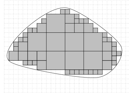
Figure 7. Dyadic Tiling

Let $C_{b}(U)$ be the totality of bounded continuous functions on $U$ and regard it as defined on $\text{\ym R}^{d}$ by zero extension.

Proposition 4.14.

$C_{b}(U)L^{1}(\text{\ym R}^{d})\subset L^{1}(\text{\ym R}^{d})$.

Proof.

Since $C_{b}(U)$ is a linear lattice, it suffices to show $hf\in L^{1}(\text{\ym R}^{d})$ for each $h\in C_{b}^{+}(U)$ and $f\in L^{1}(\text{\ym R}^{d})$. By level approximation, express $h$ as $h_{n}\uparrow h$ with $h_{n}$ positive linear combinations of bounded open sets. We know $h_{n}f\in L^{1}(\text{\ym R}^{d})$ by Corollary4.13 (i) and Proposition 4.10. The monotone convergence theorem is then applied to see $hf\in L^{1}(\text{\ym R}^{d})$. ∎

Proposition 4.15.

For a compact subset $K$ of $\text{\ym R}^{d}$, Let $C(K)$ be the set of continuous functions on $K$. Then $C^{+}(K)\subset S_{\downarrow}^{1}(\text{\ym R}^{d})$ and hence $C(K)\subset S_{\uparrow}^{1}(\text{\ym R}^{d})+S_{\downarrow}^{1}(\text{\ym R}^{d})$ by zero-extension to $\text{\ym R}^{d}\setminus K$.

Proof.

Choose an open rectangle $R$ so that $K\subset R$. Then $R\setminus K\in S_{\uparrow}^{1}(\text{\ym R}^{d})$ as a bounded open subset and $K=R-(R\setminus K)\in S(\text{\ym R}^{d})-S_{\uparrow}^{1}(\text{\ym R}^{d})=S(\text{\ym R}^{d})+S_{\downarrow}^{1}(\text{\ym R}^{d})=S_{\downarrow}^{1}(\text{\ym R}^{d})$.

Now each $f\in C^{+}(K)$ is extended to $h\in C^{+}(\text{\ym R}^{d})$ thanks to Tieze extension (Theorem A.4), which is assumed to have a comact support by replacing it with $\theta h$. Here $0\leq\theta\in C_{c}(\text{\ym R}^{d})$ satisfies $R\theta=R$.

Then $h\in C_{c}(\text{\ym R}^{d})\subset S_{\uparrow}(\text{\ym R}^{d})\cap S_{\downarrow}(\text{\ym R}^{d})$ is combined with $K\|f\|_{\infty}\in S_{\downarrow}(\text{\ym R}^{d})$ to see that $f=h\wedge(K\|f\|_{\infty})\in S_{\downarrow}(\text{\ym R}^{d})$, which is integrable in view of $I_{\downarrow}(f)\geq 0$. ∎

For a function $f$ in $C(U)$, which is positive or integrable, we write

$$\int_{\text{\ym R}^{d}}f(x)\,dx=\int_{U}f(x)\,dx\in(-\infty,\infty]$$

to indicate that $f$ is supported by $U$. Recall that the left hand side is $I_{\uparrow}(f)$ or $I^{1}(f)$ according to $f\in S_{\uparrow}(\text{\ym R}^{d})$ or $f\in L^{1}(\text{\ym R}^{d})$ respectively.

Example 4.16.

Let $\phi:U\to V$ be a bicontinuous change-of-variables, i.e., $U$ and $V$ are open subsets of $\text{\ym R}^{d}$, $\phi:U\to V$ is a bijection with $\phi$ and $\phi^{-1}$ continuous. Let $[a,b]$ be a closed rectangle included in $U$. Then, for any rectangle $R$ such that $\overline{R}=[a,b]$, say an open-closed one $(a,b]$, $\phi(R)$ is Lebesgue-integrable.

In fact, if $R=(a,b]$ for example, we can choose a sequence $(b_{n})$ of points in $U$ so that $(a,b_{n})\downarrow(a,b]$ inside $U$. Since $\phi([a,b_{n}])$ is bounded as a continuous image of $[a,b_{n}]$, $\phi((a,b])=\bigcap\phi((a,b_{n}))$ is a countable intersection of bounded open sets $\phi((a,b_{n}))$, whence $\phi((a,b])$ is Lebesgue-integrable by Corollary 4.13.

Remark 6.

There is a bicontinuous change-of-variables which does not preserve Lebesgue measurable sets.

The following are simple applications of the dominated convergence theorem.

Proposition 4.17 (Parametric continuity).

Let $f(x,t)$ be a real-valued function on $\text{\ym R}^{d}\times(a,b)$ and assume the following conditions.

1. For each $t\in(a,b)$, $f(x,t)$ is an integrable function of $x\in\text{\ym R}^{d}$.

2. For each $x\in\text{\ym R}^{d}$, $f(x,t)$ is continuous in $t\in(a,b)$.

3. There exists $g\in L^{1}(\text{\ym R}^{d})$ satisfying $|f(x,t)|\leq g(x)$.

Then $\displaystyle\int_{\text{\ym R}^{d}}f(x,t)\,dx$ is a continuous function of $t\in(a,b)$.

Proposition 4.18 (Parametric differentiability).

Let $f(x,t)$ be a function on $\text{\ym R}^{d}\times(a,b)$ satisfying the following conditions.

1. For each $t\in(a,b)$, $f(x,t)$ is integrable as a function of $x\in\text{\ym R}^{d}$,

2. For each $x\in\text{\ym R}^{d}$, $f(x,t)$ is differentiable in $t\in(a,b)$.

3. There exists $g\in L^{1}(\text{\ym R}^{d})$ satisfying $\displaystyle\left|\frac{\partial f}{\partial t}(x,t)\right|\leq g(x)$.

Then $\displaystyle\frac{\partial f}{\partial t}(x,t)$ is integrable as a function of $x$ and we have

$$\frac{d}{dt}\int_{\text{\ym R}^{d}}f(x,t)\,dx=\int_{\text{\ym R}^{d}}\frac{\partial f}{\partial t}(x,t)\,dx$$

for $a<t<b$.

Proof.

Thanks to an integral inequality

$$\left|\frac{f(x,t+h)-f(x,t)}{h}\right|=\frac{1}{|h|}\left|\int_{t}^{t+h}\frac{\partial}{\partial s}f(x,s)\,ds\right|\leq g(x)$$

for $t,t+h\in(a,b)$, we can apply the dominated convergence theorem in the limit

$$\lim_{h\to 0}\int_{\text{\ym R}^{d}}\frac{f(x,t+h)-f(x,t)}{h}\,dx$$

to get the assertion. ∎

Corollary 4.19.

Let $U\subset\text{\ym R}^{d}$ be an open subset and let a function $f$ on $U\times(a,b)$ satisfy the condition that

1. $f(x,s)$ is an integrable function of $x\in U$ for some $s\in(a,b)$,

2. $f(x,t)$ is partially differentiable with respect to $t$ for any $x\in U$,

3. $\displaystyle\frac{\partial f}{\partial t}(x,t)$ is continuous in $(x,t)\in U\times(a,b)$ and there exits an integrable $g\in C(U)$ satisfying $\displaystyle\left|\frac{\partial f}{\partial t}(x,t)\right|\leq g(x)$ ($x\in U$, $a<t<b$).

Then, for each $t\in(a,b)$, both $f(x,t)$ and $\displaystyle\frac{\partial f}{\partial t}(x,t)$ are integrable functions of $x\in U$ and $\displaystyle\int_{U}f(x,t)\,dx$ is continuously differentiable in $t\in(a,b)$ in such a way that

$$\frac{d}{dt}\int_{U}f(x,t)\,dx=\int_{U}\frac{\partial f}{\partial t}(x,t)\,dx.$$

Proof.

By (iii), $f_{t}(x,t)$ is an integrable function of $x\in U$ and satisfies

$$\left|\int_{s}^{t}\frac{\partial f}{\partial u}(x,u)\,du\right|\leq|t-s|g(x)$$

for $t\in(a,b)$. Since $\int_{s}^{t}f_{u}(x,u)\,du\in C(U)$ by Theorem 3.5, the integrability of $g$ shows that

$$f(x,t)-f(x,s)=\int_{s}^{t}\frac{\partial f}{\partial u}(x,u)\,du$$

is integrable as a function of $x\in U$ and so is $f(x,t)$ thanks to (i).

Thus all the hypotheses in parametric differentiability are satisfied and we have

$$\frac{d}{dt}\int_{U}f(x,t)\,dx=\int_{U}\frac{\partial f}{\partial t}(x,t)\,dt,$$

which is in turn continuous in $t\in(a,b)$ by parametric continuity. ∎

Example 4.20.

The gamma function

$$\Gamma(t)=\int_{0}^{\infty}x^{t-1}e^{-x}\,dx$$

is infinitely differentiable in $t>0$.

For $t=1$, $e^{-x}$ is integrable in $x>0$ and, for $0<a<1<b$,

$$\left(\frac{\partial}{\partial t}\right)^{n}x^{t-1}e^{-x}=x^{t-1}e^{-x}(\log x)^{n}$$

is continuous in $(x,t)\in(0,\infty)\times(a,b)$ and estimated by a continuous function

$$g(x)=(0,1]x^{a-1}e^{-x}|\log x|^{n}+(1,\infty)x^{b-1}e^{-x}(\log x)^{n}$$

of $x>0$. Since

$$\int_{0}^{1}x^{a-1}e^{-x}|\log x|^{n}\,dx<\infty,\quad\int_{1}^{\infty}x^{b-1}e^{-x}(\log x)^{n}\,dx<\infty,$$

$g$ is integrable and the hyptheses in Corollary are fulfilled.

Exercise 23.

Show the integrability of $g$.

Example 4.21.

Differentiation of $\displaystyle\int_{0}^{\infty}\frac{dx}{t+x^{2}}=\frac{\pi}{2\sqrt{t}}$ ($t>0$) gives

$$\int_{0}^{\infty}\frac{dx}{(t+x^{2})^{n+1}}=\frac{\pi}{2t^{n}\sqrt{t}}\frac{(2n-1)!!}{(2n)!!}\quad(n=1,2,\cdots).$$

Exercise 24.

Find a dominating function of each integrand.

For a later use in §8, we describe partitions of unity in the present context. Let $A\subset\text{\ym R}^{d}$ be a Lebesgue measurable set and $\rho\in C_{c}^{+}(\text{\ym R}^{d})$ be a probability density function on $\text{\ym R}^{d}$, i.e., $\int\rho(x)\,dx=1$. Then, for the translation $\rho_{x}(y)=\rho(y-x)$ of $\rho$ by $x\in\text{\ym R}^{d}$, $A\rho_{x}$ is integrable and

$$A^{\rho}(x)\equiv\int_{A}\rho(y-x)\,dy=\int_{(A-x)\cap[\rho>0]}\rho(y)\,dy\in[0,1]$$

(a moving average of $A$) is continuous as a function of $x\in\text{\ym R}^{d}$ by parametric continuity, which is in the class $C^{n}$ if so is $\rho$ by parametric differentiability.

From the last equality, one sees that $A^{\rho}$ vanishes outside an open set $A-[\rho>0]=\bigcup_{a\in A}(a-[\rho>0])$ and $A^{\rho}(x)=1$ if $x+[\rho>0]\subset A$. Thus, if $\rho$ satisfies $[\rho>0]\subset B_{r}(0)$, then

$$\{x\in\text{\ym R}^{d};B_{r}(x)\subset A\}\leq A^{\rho}\leq\bigcup_{a\in A}B_{r}(a).$$

Here $B_{r}(a)=\{x\in\text{\ym R}^{d};|x-a|<r\}$ denotes an open ball of radius $r>0$ at $a\in\text{\ym R}^{d}$ This is especially useful when $r>0$ is small. In that case, $\rho$ approximately representes the so-called delta function.

To rewite these inequalities in a more convenient form , we introduce one more notation: For a non-empty subset $A\subset\text{\ym R}^{d}$, let $d_{A}:\text{\ym R}^{d}\to[0,\infty)$ be the distance function from $A$ defined by $d_{A}(x)=\inf\{|x-a|;a\in A\}$, which is continuous and satisfies $d_{A}(x)=0\iff x\in\overline{A}$.

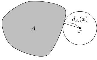
Figure 8. Distance Function

Proposition 4.22 (partition of unity).

Given a finite open covering $(U_{i})_{1\leq i\leq l}$ of a compact set $K$ in $\text{\ym R}^{d}$, we can find functions $h_{i}\in C_{c}^{+}(\text{\ym R}^{d})$ satisfying $[h_{i}]\subset U_{i}$, $\sum_{i}h_{i}\leq 1$ and $\sum_{i}h_{i}=1$ on $K$.

Proof.

For each $a\in K$, choose $i$ and then $r>0$ so that $\overline{B_{r}}(a)\subset U_{i}$ and then cover $K$ by $B_{r}(a)$. (Here $\overline{B_{r}}(a)=\{x\in\text{\ym R}^{d};|x-a|\leq r\}$ denotes a closed ball of radius $r>0$.) By compactness of $K$, we can find a finite covering $(B_{r_{j}}(a_{j})$ in such a way that, for each $j$, there is an $i$ satisfying $\overline{B_{r_{j}}}(a_{j})\subset U_{i}$. In the former covering inclusion and the latter localized inclusion, one sees that $[d_{K}\leq\delta]\subset\bigcup_{j}B_{r_{j}}(a_{j})$ and $\overline{B_{r_{j}+\delta}}(a_{j})\subset U_{i}$ for sufficiently small $\delta>0$.

Now let $B_{j}$ be inductively defined by

$$B_{r_{1}}(a_{1})\cup\dots\cup B_{r_{j}}(a_{j})=B_{1}\sqcup B_{2}\sqcup\dots\sqcup B_{j}\quad(j=1,2,\dots).$$

and an approximate delta function $\rho\in C_{c}^{\infty}(\text{\ym R}^{d})$ be supported by $B_{\delta}(0)$. Then, $B_{j}^{\rho}$ satisfies $[B_{j}^{\rho}]\subset\overline{B_{r_{j}+\delta}}(a_{j})\subset U_{i}$, $0\leq\sum_{j}B_{j}^{\rho}\leq 1$ and $\sum_{j}B_{j}^{\rho}=1$ on $K$.

Finally, partition $\{j\}$ into $\bigsqcup_{i}J_{i}$ (possibly $J_{i}=\emptyset$) so that $[B_{j}^{\rho}]\subset U_{i}$ ($j\in J_{i}$), partial sums $h_{i}=\sum_{j\in J_{i}}B_{j}^{\rho}$ meet the conditions. ∎

5. Null Functions and Null Sets

Exceptional sets mentioned in §3 are now clearly and firmly described as null sets. A function $f:X\to[-\infty,\infty]$ is said to be null or negligible if $\overline{I}(|f|)=0$. In view of $0\leq\underline{I}(|f|)\leq\overline{I}(|f|)$, a real-valued function $f$ is null if and only if $f\in L^{1}$ and $I^{1}(|f|)=0$. A subset $A\subset X$ is null or negligible if so is the indicator function of $A$, i.e., $\overline{I}(A)=I^{1}(A)=0$.

Here are simple properties of negligibleness.

Proposition 5.1.

1. If $|f|\leq g$ with $g$ a null function, then $f$ is a null function. In particular, a subset of a null set is null.

2. If $(f_{n})$ is a sequence of positive null functions, $\sum f_{n}$ is a null function. Likewise, if $(A_{n})$ is a sequence of null sets, the union $\bigcup A_{n}$ is a null set.

3. $f$ is a null function if and only if $[f\not=0]$ is a null set.

Proof.

(i) follows from the monotonicity of $\overline{I}$.

(ii) follows from the subadditivity of $\overline{I}$ and $\bigcup A_{n}\leq\sum A_{n}$.

(iii) If $f$ is a null function, $\infty|f|=|f|+|f|+\cdots$ is null as well and $[f\not=0]\leq\infty|f|$ shows that $[f\not=0]$ is a null set. Conversely, if $[f\not=0]$ is a null set, $\infty|f|=[f\not=0]+[f\not=0]+\cdots$ is a null function and hence so is $|f|\leq\infty|f|$. ∎

As a consequence of (iii), we observe that, for an integrable function $f$, its integral $I^{1}(f)$ as well as integrability remains unchanged when $f$ is modified on a null set.

For functions $f,g:X\to[-\infty,\infty]$, we write $f\;\mathring{\leq}\;g$ if $[f>g]$ is a null set, which is a semi-order relation among $\overline{\text{\ym R}}$-valued functions with the associated equivalence relation denoted by $f\;\mathring{=}\;g$. Note that $f\;\mathring{=}\;g$, i.e., $f\;\mathring{\leq}\;g$ and $g\;\mathring{\leq}\;f$, means that $[f\not=g]$ is a null set.

More generally a condition $P$ on an element in the base set $X$ of an integral system $(L,I)$ is almost satisfied if $X\setminus[P]$ is a null set.

It is then customary and very useful to talk integrability about functions which are well-defined on $X\setminus N$ with $N$ a null set: A function $f$ is integrable in this (extended) sense and write $f\mathring{\in}L^{1}$ if there exists $g\in L^{1}$ such that $f\;\mathring{=}\;g$, with its integral $I^{1}(f)$ well-defined by $I^{1}(g)$.

Example 5.2.

$\log|x|$ is locally integrable as a function of $x\in\text{\ym R}$ and its indefinite integral (not a primitive function) is given by a continuous function $x\log|x|-x+C$.

Exercise 25.

Check this fact.

The monotone convergence theorem is now strengthened as follows.

Theorem 5.3.

Let $(f_{n})$ be an increasing sequence in $L^{1}$ with $f=\lim f_{n}$ and assume that $\displaystyle\lim_{n\to\infty}I^{1}(f_{n})<\infty$. Then $[f=\infty]$ is a null set and $[f<\infty]f$ is integrable so that $\displaystyle I^{1}([f<\infty]f)=\lim_{n\to\infty}I^{1}(f_{n})$.

Proof.

Let $g_{n}=f_{n+1}-f_{n}\in L^{1}$ so that $f-f_{1}=\sum_{n\geq 1}g_{n}$. Then, thanks to the subadditivity of upper integrals,

$$\overline{I}(f-f_{1})\leq\sum_{n\geq 1}\overline{I}(g_{n})=\sum_{n\geq 1}I^{1}(g_{n})=\lim_{n\to\infty}I^{1}(\sum_{j=1}^{n}g_{j})=\lim_{n\to\infty}I^{1}(f_{n}-f_{1}),$$

which is combined with the monotonicity $\lim I^{1}(f_{n}-f_{1})=\lim\overline{I}(f_{n}-f_{1})\leq\overline{I}(f-f_{1})$ to get the equality $\overline{I}(f-f_{1})=\lim I^{1}(f_{n}-f_{1})$.

Here $[f-f_{1}=\infty]\leq r(f-f_{1})$ ($r>0$) is used to have

$$\overline{I}([f-f_{1}=\infty])\leq r\overline{I}(f-f_{1})=r\lim_{n\to\infty}I^{1}(f_{n}-f_{1})=r(\lim_{n\to\infty}I^{1}(f_{n})-I^{1}(f_{1})).$$

Since $I_{\uparrow}(f)<\infty$ and $r>0$ is arbitrary, this implies that $[f=\infty]=[f-f_{1}=\infty]$ is a null set and then $[f<\infty]f_{n}\in L^{1}$ satisfies $I^{1}([f<\infty]f_{n})=I^{1}(f_{n})$ as a modification by a null function.

Now the original monotone convergence theorem is applied to $[f<\infty]f_{n}\uparrow[f<\infty]f$ with $\displaystyle\lim_{n\to\infty}I^{1}([f<\infty]f_{n})=\lim_{n\to\infty}I^{1}(f_{n})<\infty$ to see that $[f<\infty]f$ is integrable and

$$I^{1}([f<\infty]f)=\lim I^{1}([f<\infty]f_{n})=\lim I^{1}(f_{n}).$$

∎

Corollary 5.4.

Let $f_{j}\in L_{\uparrow}$ satisfy $I_{\uparrow}(f_{j})<\infty$ ($j=1,2$). Then $[f_{j}=\infty]$ ($j=1,2$) are null sets, $[f_{1}\wedge f_{2}<\infty]f_{j}$ is integrable and $I^{1}([f_{1}\wedge f_{2}<\infty]f_{1}-[f_{1}\wedge f_{2}<\infty]f_{2})=I_{\uparrow}(f_{1})-I_{\uparrow}(f_{2})$.

Exercise 26.

Let $f:X\to(-\infty,\infty]$ satisfy $f_{n}\uparrow f$ with $f_{n}\in L^{1}$. Then $\overline{I}(f)=\lim_{n\to\infty}I^{1}(f_{n})$.

At this point, we have various monotone extensions of $L$ between $L^{1}\cap L_{\uparrow}$ and $L^{1}_{\uparrow}=(L^{1})_{\uparrow}$:

$$\{f\in L_{\uparrow};I_{\uparrow}(f)<\infty\},$$

$$\{f:X\to\text{\ym R};f\,\mathring{\in}\,L_{\uparrow}\},$$

$$\{f:X\to\text{\ym R};f\,\mathring{\in}\,L_{\uparrow},I^{1}_{\uparrow}(f)<\infty\}$$

and so on. Among these, the last one is interesting because every integrable function is a difference of functions belonging to this class (see Appendix B), whereas the first one is practically useful because concrete integrable functions are differences of functions in this class as seen by Corollary 5.4, which shall be utilized in repeated integrals discussed in the next section.

6. Repeated Integrals Revisited

Historically a reasonable formulation of the subject had not been apparent for a while and it was crucial to allow exceptional points which constitute a null set. We here present a practical form of the so-called Fubini theorem without getting much involved in measurability.

Let $d=d^{\prime}+d^{\prime\prime}$ and express $x\in\text{\ym R}^{d}$ by $x=(x^{\prime},x^{\prime\prime})$ with $x^{\prime}\in\text{\ym R}^{d^{\prime}}$ and $x^{\prime\prime}\in\text{\ym R}^{d^{\prime\prime}}$. For $A\subset\text{\ym R}^{d}$, let $A^{\prime}\subset\text{\ym R}^{d^{\prime}}$ ($A^{\prime\prime}\subset\text{\ym R}^{d^{\prime\prime}}$) be the projection of $A$ to the $d^{\prime}$-component ($d^{\prime\prime}$-component) respectively and the cut of $A$ by $x^{\prime}\in\text{\ym R}^{d^{\prime}}$ ($x^{\prime\prime}\in\text{\ym R}^{d^{\prime\prime}}$) is defined to be $A_{x^{\prime}}=\{a^{\prime\prime}\in\text{\ym R}^{d^{\prime\prime}};(x^{\prime},a^{\prime\prime})\in A\}$ ($A_{x^{\prime\prime}}=\{a^{\prime}\in\text{\ym R}^{d^{\prime}};(a^{\prime},x^{\prime\prime})\in A\}$). Thus $A^{\prime}=\{x^{\prime}\in\text{\ym R}^{d^{\prime}};A_{x^{\prime}}\not=\emptyset\}$.

Note that, for an open set $U$, cuts $U_{x^{\prime}}$, $U_{x^{\prime\prime}}$ as well as projections $U^{\prime}$, $U^{\prime\prime}$ are open sets.

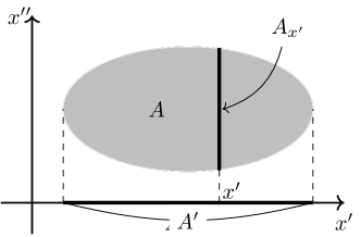
Figure 9. Cut and Projection

Proposition 3.3 is here paraphrased as follows.

Lemma 6.1.

Let $f\in S_{\uparrow}(\text{\ym R}^{d})$. Then, for each $x^{\prime}\in\text{\ym R}^{d^{\prime}}$, $f(x^{\prime},\cdot)\in S_{\uparrow}(\text{\ym R}^{d^{\prime\prime}})$ and $\int f(x^{\prime},x^{\prime\prime})\,dx^{\prime\prime}$ belongs to $S_{\uparrow}(\text{\ym R}^{d^{\prime}})$ as a function of $x^{\prime}$ in such a way that

$$\int f(x)\,dx=\int dx^{\prime}\,\int f(x^{\prime},x^{\prime\prime})\,dx^{\prime\prime}.$$

Proposition 6.2.

A continuous function $f$ defined on an open set $U\subset\text{\ym R}^{d}$ is integrable if and only if

$$\int_{U^{\prime}}dx^{\prime}\int_{U_{x^{\prime}}}|f(x^{\prime},x^{\prime\prime})|\,dx^{\prime\prime}<\infty.$$

Moreover if this is the case, we have

$$\int_{U}f(x)\,dx=\int_{U^{\prime}}dx^{\prime}\int_{U_{x^{\prime}}}f(x^{\prime},x^{\prime\prime})\,dx^{\prime\prime}.$$

Here $f(x^{\prime},\cdot)$ belongs to $L^{1}(\text{\ym R}^{d^{\prime\prime}})$ for almost all $x^{\prime}\in U^{\prime}$ and $\displaystyle\int_{U_{x^{\prime}}}f(x^{\prime},x^{\prime\prime})\,dx^{\prime\prime}$ is integrable as a function of $x^{\prime}\in U^{\prime}$.

Proof.

Write $f=f\vee 0-(-f)\vee 0$ with $(\pm f)\vee 0\in C^{+}(U)$ and apply the above lemma to $(\pm f)\vee 0$ in view of $C^{+}(U)\subset S_{\uparrow}(\text{\ym R}^{d})$ (Proposition 4.12 (ii)).

The assertion then follows as their difference, where an ‘almost’ argument, together with Theorem 5.3, is used to dispose of the $\infty-\infty$ ambiguity. ∎

Corollary 6.3.

Let $\varphi\leq\psi$ be continuous functions on an open interval $(a,b)$ and $D=\{(x,y);a<x<b,\varphi(x)<y<\psi(x)\}\in S_{\uparrow}(\text{\ym R}^{2})$ be an open domain bordered by $\varphi$ and $\psi$ (a graph region).

Then, for a continuous function $f$ on $D$, $D|f|\in S_{\uparrow}(\text{\ym R}^{2})$ and its integral $I_{\uparrow}(D|f|)$ is calculated by

$$\int_{D}|f|=\int_{a}^{b}dx\,\int_{\varphi(x)}^{\psi(x)}|f(x,y)|\,dy$$

so that this is finite if and only if $Df\in L^{1}(\text{\ym R}^{2})$. Moreover, if this is the cse,

$$I^{1}(Df)=\int_{D}f=\int_{a}^{b}dx\,\int_{\varphi(x)}^{\psi(x)}f(x,y)\,dy,$$

In particular, for the choice $f\equiv 1$, the Lebesgue measure $|D|$ of $D$ is expressed by a one-variable integral

$$|D|=\int_{a}^{b}(\psi(x)-\varphi(x))\,dx,$$

which is exactly the area formula of $D$ in the elementary calculus.

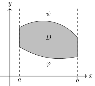
Figure 10. Graph Region

Example 6.4.

When $(a,b)$ is bounded and $\phi:(a,b)\to\text{\ym R}$ is a continuous function, the choice $\varphi=\phi-\delta$ and $\psi=\phi+\delta$ with $\delta>0$ gives

$$|D|=\int_{a}^{b}2\delta\,dx=2\delta(b-a)\downarrow 0\quad(\delta\downarrow 0).$$

Thus the graph $\{(x,\phi(x));a<x<b\}\subset\text{\ym R}^{2}$ of $\phi$, which is included in $D$ for any $\delta>0$, is a null set.

Example 6.5.

Consider the repeated integral of $e^{-(1+x^{2})y}$ supported by the first quadrant $(0,\infty)^{2}\subset\text{\ym R}^{2}$. In terms of the half Gaussian integral $C=\int_{0}^{\infty}e^{-x^{2}}\,dx$, this is

$$\int_{x>0,y>0}e^{-(1+x^{2})y}\,dxdy=\int_{0}^{\infty}dy\,e^{-y}\int_{0}^{\infty}e^{-yx^{2}}\,dx=C\int_{0}^{\infty}e^{-y}\frac{1}{\sqrt{y}}\,dy=2C^{2},$$

which is equal to

$$\int_{0}^{\infty}dx\,\int_{0}^{\infty}e^{-(1+x^{2})y}\,dy=\int_{0}^{\infty}\frac{1}{x^{2}+1}\,dx=\frac{\pi}{2}.$$

Thus

$$\int_{0}^{\infty}e^{-x^{2}}\,dx=\frac{\sqrt{\pi}}{2}.$$

Example 6.6 (Dirichlet integral).

From repeated integrals of the double integral $\displaystyle\int_{x>0,y>r}e^{-xy}\sin x\,dxdy$ ($r>0$), we have

$$\int_{0}^{\infty}e^{-rx}\frac{\sin x}{x}\,dx=\frac{\pi}{2}-\arctan r,$$

which is the Laplace transform of $\operatorname{sinc}(x)=(\sin x)/x$ ($x>0$) and its continuity at $r=+0$ (Theorem 2.27) takes the form

$$\int_{0}^{\infty}\frac{\sin x}{x}\,dx=\frac{\pi}{2}.$$

7. Jacobian Formula

To fully appreciate the power of repeated integrals, we here establish the change-of-variables formula in multiple integrals.

Theorem 7.1 (Transfer Principle).

Let $(L,I)$, $(M,J)$ be integral systems on sets $X$, $Y$ respectively, $\rho:X\to[0,\infty)$ be a function on $X$ and $\phi:X\to Y$ be a map satisfying $\rho(M\circ\phi)\subset L$ and $I(\rho(g\circ\phi))=J(g)$ ($g\in M$).

Then we have $\rho(M^{1}\circ\phi)\subset L^{1}$ and $I^{1}(\rho(g\circ\phi))=J^{1}(g)$ ($g\in M^{1}$) for their Daniell extensions.

Proof.

We just check $\rho(M_{\uparrow}\circ\phi)\subset L_{\uparrow}$, $I_{\uparrow}(\rho(g\circ\phi))=J_{\uparrow}(g)$ ($g\in M_{\uparrow}$) and so on, step by step. Details are left to the reader. ∎

Corollary 7.2.

1. If $\phi:X\to Y$ is bijective and $L=M\circ\phi$, we have $L^{1}=M^{1}\circ\phi$ and $J^{1}(g)=I^{1}(g\circ\phi)$ ($g\in M^{1}$).

2. If integral systems $(L,I)$, $(M,J)$ on a set $X$ satisfy $L\subset M$, $J|_{L}=I$, i.e., $(M,J)$ is an extension of $(L,I)$, then $L^{1}\subset M^{1}$ and $J^{1}$ on $M^{1}$ is an extension of $I^{1}$ on $L^{1}$.

Example 7.3.

For $f\in L^{1}(\text{\ym R}^{d})$ and $y\in\text{\ym R}^{d}$, $f(x+y)$ is integrable as a function of $x\in\text{\ym R}^{d}$ and

$$\int_{\text{\ym R}^{d}}f(x+y)\,dx=\int_{\text{\ym R}^{d}}f(x)\,dx.$$

This follows from translational invariance of the volume functional.

Exercise 27.

For a function $f\in L^{1}(\text{\ym R}^{d})$ and a positive real $r>0$, check the identity

$$\int_{\text{\ym R}^{d}}f(rx)\,dx=r^{-d}\int_{\text{\ym R}^{d}}f(x)\,dx.$$

Example 7.4.

For an open set $U\subset\text{\ym R}^{d}$, consider a continuous function $f$ supported by a compact subset of $U$ and let $C_{c}(U)$ be the totality of such functions, which is identified with $\{f\in C_{c}(\text{\ym R}^{d});Uf=f\}$ by the obvious inclusion $C_{c}(U)\subset C_{c}(\text{\ym R}^{d})$ and set $S(U)=\{f\in S(\text{\ym R}^{d});Uf=f\}$. These are linear sublattices of $L^{1}(\text{\ym R}^{d})$ and the volume integral (or the Lebesgue integral) is restricted to provide integral systems. Their Daniell extensions are then realized as restrictions of $I^{1}$ to $C_{c}(U)^{1}\subset L^{1}(\text{\ym R}^{d})$ and $S(U)^{1}\subset L^{1}(\text{\ym R}^{d})$ respectively.

Moreover, in view of $S(U)\subset C_{c}(U)^{1}$ and $C_{c}(U)\subset S(U)^{1}$, the maximality of Daniell extension reveals that $S^{1}(U)\subset C_{c}(U)^{1}$ and $C_{c}(U)^{1}\subset S(U)^{1}$, i.e., $C_{c}(U)^{1}=S(U)^{1}$, which is denoted by $L^{1}(U)$.

Based on this fact, we henceforth regard $L^{1}(U)$ as a Daniell extension of $C_{c}(U)$ relative to the volume integral.

Exercise 28.

Show that $S(U)\subset C_{c}(U)^{1}$ and $C_{c}(U)\subset S(U)^{1}$. Hint: $S(U)$ and $C_{c}(U)$ are mutually approximated by doubly bounded seqeuncial limits.

Proposition 7.5.

For an open subset $U$ of $\text{\ym R}^{d}$, $L^{1}(U)=UL^{1}(\text{\ym R}^{d})$. In particular, $UL^{1}(\text{\ym R}^{d})\subset L^{1}(\text{\ym R}^{d})$.

Proof.

Not obvious is the inclusion $UL^{1}(\text{\ym R}^{d})\subset L^{1}(U)$, which follows from Proposition 4.10 and Corollary 4.13 (i). ∎

Remark 7.

By a $\sigma$-induction (i.e., a monotone class argument) with measure-theoretical completion accompanied, one can generalize the last cutting property to arbitrary Lebesgue measurable sets.

Exercise 29.

Let $U$ be a bounded open set of $\text{\ym R}^{d}$ and $f$ be a bounded continuous function on $U$. Then $f\in L^{1}(U)$.

We now state our goal (Jacobian formula) in this section as follows.

Theorem 7.6.

Let $U$, $V$ be open subsets of $\text{\ym R}^{d}$ and $\phi:U\to V$ be a smooth change-of-variables, i.e., $\phi$ is bijective with $\phi$ and $\phi^{-1}$ differentiable and the derivative $\phi^{\prime}:U\to M_{d}(\text{\ym R})$ of $\phi$ continuous. Note that $\phi^{\prime}(x)$ is an invertible matrix for each $x\in U$.

Then, for $g\in C_{c}(V)\cup C^{+}(V)$,

$$\int_{V}g(y)\,dy=\int_{U}g(\phi(x))|\det(\phi^{\prime}(x))|\,dx.$$

As an immediate consequence of the transfer principle, the Jacobian formula remains valid even for $g\in L^{1}(V)$.

Corollary 7.7.

A function $g$ on $V$ is Lebesgue integrable (Legesgue negligible) if and only if so is $(g\circ\phi)|\det(\phi^{\prime})|$ on $U$ ($g\circ\phi$ on $U$).

Remark 8.

Nowadays, there seems some confusion in what Jacobian means. In view of historical flow, it was used (and is still used) to express $\det(\phi^{\prime}(x))$ but a recent usage is widened to refer to its absolute value as well or even the differential matrix $\phi^{\prime}(x)$.

Proposition 7.8.

A smooth change-of-variables preserves Lebesgue measurable sets as well as Lebesgue null sets.

Proof.

Let $\phi:U\to V$ be a smooth change-of-variables and $B\subset V$ be Lebesgue measurable. Since $|\det\phi^{\prime}|^{-1}$ is a continuous function on $U$, we can find a sequence $h_{n}\in C_{c}^{+}(U)$ so that $h_{n}\uparrow|\det\phi^{\prime}|^{-1}$. Then

$$(B\circ\phi)|\det\phi^{\prime}|h_{n}\in L^{1}(U)C_{c}(U)\subset L^{1}(U)$$

(Proposition 4.14) and $h_{n}(B\circ\phi)|\det\phi^{\prime}|\uparrow B\circ\phi$ shows that $B\circ\phi\in L^{1}_{\uparrow}(U)$, i.e., $B\circ\phi=\phi^{-1}(B)$ is Lebesgue measurable (Proposition 4.9 (i)).

For a null set $B$, $\int_{U}(B\circ\phi)|\det\phi^{\prime}|=\int_{V}B=|B|=0$ and $\phi^{-1}(B)=[(B\circ\phi)|\det\phi^{\prime}|>0]$ is a null set by Proposition 5.1 (iii). ∎

Proof of Jacobian Formula

We first establish the special case when $\phi:\text{\ym R}^{d}\to\text{\ym R}^{d}$ is realized by a matrix multiplication: Let $T$ be an invertible matrix of size $d$. Then for $f\in C_{c}(\text{\ym R}^{d})$ and hence for $f\in L^{1}(\text{\ym R}^{d})$ by the transfer principle,

$$\int f(Tx)\,dx=|\det T|^{-1}\int f(x)\,dx.$$

Remark here that under an invertible linear transformation of variables $C_{c}(\text{\ym R}^{d})\subset S_{\uparrow}(\text{\ym R}^{d})\cap S_{\downarrow}(\text{\ym R}^{d})$ is invariant, whereas $S_{\uparrow}(\text{\ym R}^{d})\cap S_{\downarrow}(\text{\ym R}^{d})$ is not as noticed before.

Since any invertible matrix is a product of elementary ones and the volume integral is permutation-invariant, the repeated integral formula on $S_{\uparrow}(\text{\ym R}^{d})\cap S_{\downarrow}(\text{\ym R}^{d})$ reduces the problem to checking it for two-dimensional matrices

$$\begin{pmatrix}\alpha&0\\ 0&\beta\end{pmatrix},\quad\begin{pmatrix}1&\gamma\\ 0&1\end{pmatrix},$$

where $\alpha,\beta\in\text{\ym R}^{\times}$ and $\gamma\in\text{\ym R}$.

For these, the scale covariance and the translational invariance of the width integral are combined with repeated integrals to conclude as follows:

$$\int_{\text{\ym R}^{2}}f(\alpha x,\beta y)\,dxdy=\frac{1}{|\alpha||\beta|}\int_{\text{\ym R}^{2}}f(x,y)\,dxdy.$$

$$\int_{\text{\ym R}^{2}}f(x+\gamma y,y)\,dxdy =\int_{\text{\ym R}}dy\int_{\text{\ym R}}f(x+\gamma y,y)\,dx$$

$$(\text{by the translational invariance of $\int dx$})$$

$$=\int_{\text{\ym R}}dy\int_{\text{\ym R}}f(x,y)\,dx=\int_{\text{\ym R}^{2}}f(x,y)\,dxdy.$$

Next we go on to the non-linear case after J. Schwartz[6]. For the Jacobian formula on $C_{c}(V)$, it is enough to show the validity for $g\in C_{c}^{+}(V)$, which in turn implies the case $C^{+}(V)$ because each $g\in C^{+}(V)$ is expressed in the form $g_{n}\uparrow g$ with $g_{n}\in C_{c}^{+}(V)$.

To establish the formula on $C_{c}^{+}(V)$, we need some notations in norm estimates. For a numerical vector $x=(x_{1},\dots,x_{d})\in\text{\ym R}^{d}$ and a real matrix $A=(a_{i,j})_{1\leq i,j\leq d}$, set

$$\|x\|_{\infty}=\max_{1\leq i\leq d}\{|x_{i}|\},\quad\|A\|=\max_{1\leq i\leq d}\{\sum_{j=1}^{d}|a_{i,j}|\},$$

where $\|A\|$ is the operator norm relative to $\|\cdot\|_{\infty}$ and satisfies inequalities $\|Ax\|_{\infty}\leq\|A\|\|x\|_{\infty}$, $\|AB\|\leq\|A\|\|B\|$.

Exercise 30.

Check these inequalities.

Let $[a,b]$ ($b_{1}-a_{1}=\dots=b_{d}-a_{d}=2r$) be a $d$-dimensional closed cube contained in $U$. From the fundamental formula in calculus, we have

$$\phi(x)-\phi(c)=\sum_{j=1}^{d}\int_{0}^{1}dt\,\frac{\partial\phi}{\partial x_{j}}(tx+(1-t)c)(x_{j}-c_{j})$$

and then

$$\|\phi(x)-\phi(c)\|_{\infty}\leq\|x-c\|_{\infty}\max_{0\leq t\leq 1}\|\phi^{\prime}(tx+(1-t)c)\|$$

for $x,c\in[a,b]$.

In particular, choosing $c=(a+b)/2$, we see that $\phi([a,b])$ is included in the closed cube of center $c$ and width $2r\|\phi^{\prime}\|_{[a,b]}$, whence

$$|\phi((a,b])|\leq\|\phi^{\prime}\|_{[a,b]}^{d}(2r)^{d}=\|\phi^{\prime}\|_{[a,b]}^{d}|(a,b]|,$$

where, for a subset $C\subset U$, $\|\phi^{\prime}\|_{C}=\sup\{\|\phi^{\prime}(x)\|;x\in C\}$. Recall that $\phi((a,b])$ is a Lebesgue integrable set (Example 4.16).

Invoking the chain rule $(\phi^{\prime}(c)^{-1}\phi)^{\prime}=\phi^{\prime}(c)^{-1}\phi^{\prime}$, the above estimate applied to $\phi^{\prime}(c)^{-1}\phi:U\to\phi^{\prime}(c)^{-1}(V)$ takes the form

$$|\phi((a,b])|=|\det\phi^{\prime}(c)||\phi^{\prime}(c)^{-1}\phi((a,b])|\leq|\det\phi^{\prime}(c)||\phi^{\prime}(c)^{-1}\phi^{\prime}\|_{[a,b]}^{d}|(a,b]|.$$

Let $f=g\circ\phi\in C_{c}^{+}(U)$ and divide $[a,b]$ into a multiple partition $\Delta$ so that $(a,b]$ is a disjoint union of open-closed subcubes $(R_{i})_{1\leq i\leq m}$ of width $2r_{i}$ and apply the above inequality for each $R_{i}$ with the center $\xi_{i}$ of $R_{i}$ as a sample point to have

$$I^{1}(f_{\Delta,\xi}\circ\phi^{-1})=\sum_{i}f(\xi_{i})|\phi(R_{i})|\leq\sum_{i}f(\xi_{i})|\det\phi^{\prime}(\xi_{i})||\phi^{\prime}(\xi_{i})^{-1}\phi^{\prime}\|_{R_{i}}^{d}|R_{i}|.$$

Note here that $\phi(R_{i})=R_{i}\circ\phi^{-1}$ as indicator functions and hence $|\phi(R_{i})|=I^{1}(R_{i}\circ\phi^{-1})$.

Now let $m\to\infty$ so that $r_{i}\to 0$ uniformly in $i$. Then $f_{\Delta,\xi}$ converges uniformly to $(a,b]f$ and the dominated convergence theorem gives

$$\lim I^{1}(f_{\Delta,\xi}\circ\phi^{-1})=I^{1}(((a,b]f)\circ\phi^{-1}) =I^{1}(\phi((a,b])(f\circ\phi^{-1}))$$

$$=\int_{\phi((a,b])}f(\phi^{-1}(y))\,dy.$$

In the right hand side, $\phi^{\prime}(\xi_{i})^{-1}\phi^{\prime}(x)$ ($x\in{R_{i}}$) converges to the identity matrix uniformly, which is combined with the Cauchy-Riemann-Darboux formula to have

$$\lim\sum_{i}f(\xi_{i})|\det\phi^{\prime}(\xi_{i})||\phi^{\prime}(\xi_{i})^{-1}\phi^{\prime}\|_{R_{i}}^{d}|R_{i}|=\int_{(a,b]}f(x)|\det\phi^{\prime}(x)|\,dx,$$

concluding that

$$\int_{\phi((a,b])}g(y)\,dy\leq\int_{(a,b]}g(\phi(x))|\det\phi^{\prime}(x)|\,dx.$$

To put this together, express $U$ as a countable disjoint union of dyadic cubes $(a,b]$ satisfying $[a,b]\subset U$ so that $f=\sum(a,b]f$. Since $g\in C_{c}^{+}(V)$ is integrable, we can apply the dominated onvergence theorem to the expression $\sum((a,b]f)\circ\phi^{-1}=f\circ\phi^{-1}=g$ to have

$$\int_{V}g(y)\,dy=\sum\int_{\phi((a,b])}g(y)\,dy \leq\sum\int_{(a,b]}g(\phi(x))|\det\phi^{\prime}(x)|\,dx$$

$$=\int_{U}g(\phi(x))|\det\phi^{\prime}(x)|\,dx.$$

Since the last integrand $h$ is in $C_{c}^{+}(U)$, $\phi^{-1}:V\to U$ is applied for $h$, together with the chain rule $\phi^{\prime}(\phi^{-1}(y))(\phi^{-1})^{\prime}(y)=(\phi\circ\phi^{-1})^{\prime}(y)=\text{id}$, to obtain the reverse inequality

$$\int_{U}g(\phi(x))|\det\phi^{\prime}(x)|\,dx\leq\int_{V}g(y)\,dy,$$

proving the Jacobian formula for $g\in C_{c}^{+}(V)$.

Exercise 31.

Check the integrability of $\phi((a,b])g$ when $[a,b]\subset U$. Hint: Express $(a,b_{n})\downarrow(a,b]$ and notice that $\phi(a,b_{n})g$ is integrable.

Remark 9.

If we use the technique of partition of unity concerning open coverings, we can dispense with convergence theorems in Lebesgue integrals and complete the whole proof within Cauchy-Riemann integrals.

Example 7.9.

Let $n=2$ and $\phi:(0,\infty)\times(-\pi,\pi)\to\text{\ym R}^{2}\setminus(-\infty,0]\times\{0\}$ be the polar coordinate transformation $\phi(r,\theta)=(r\cos\theta,r\sin\theta)$. Here old variables are $(r,\theta)$ and we regard $(x,y)$ as new variables. Then

$$\det(\phi^{\prime}(r,\theta))=\begin{vmatrix}\cos\theta&-r\sin\theta\\ \sin\theta&r\cos\theta\end{vmatrix}=r$$

and, if an open set $U\subset(0,\infty)\times(-\pi,\pi)$ is transformed into an open set $V\subset\text{\ym R}^{2}\setminus(-\infty,0]\times\{0\}$ by $\phi$, the equality

$$\int_{V}g(x,y)\,dxdy=\int_{U}g(r\cos\theta,r\sin\theta)\,rdrd\theta$$

holds for $g\in C^{+}(V)$. Thus, if $f\in C(V)$ satisfies $|f|\leq g$ with

$$\int_{U}g(r\cos\theta,r\sin\theta)\,rdrd\theta<\infty,$$

then $f\in L^{1}(V)$ and

$$\int_{V}f(x,y)\,dxdy=\int_{U}f(r\cos\theta,r\sin\theta)\,rdrd\theta.$$

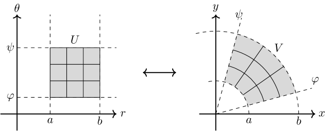
Figure 11. Polar Coordinates

Example 7.10.

Let $C=\int_{-\infty}^{\infty}e^{-t^{2}}\,dt$ and $N=(-\infty,0]\times\{0\}\subset\text{\ym R}^{2}$. Then $N$ is a closed null set in $\text{\ym R}^{2}$ and

$$C^{2} =\int_{\text{\ym R}^{2}}e^{-(x^{2}+y^{2})}\,dxdy=\int_{\text{\ym R}^{2}\setminus N}e^{-(x^{2}+y^{2})}\,dxdy$$

$$=\int_{(0,\infty)\times(-\pi,\pi)}e^{-r^{2}}r\,drd\theta=\int_{0}^{\infty}e^{-r^{2}}r\,dr\int_{-\pi}^{\pi}d\theta$$

$$=\pi\int_{0}^{\infty}e^{-r^{2}}d(r^{2})=\pi,$$

showing $C=\sqrt{\pi}$ again.

As a popular application, we shall express the beta function in terms of the gamma function.

Recall that the gamma function is defined by

$$\Gamma(t)=\int_{0}^{\infty}x^{t-1}e^{-x}\,dx=2\int_{0}^{\infty}x^{2t-1}e^{x^{2}}\,dx\quad(t>0),$$

which is a continuous replacement of factorial in the sense that $(t-1)!=\Gamma(t)$. The beta function is defined by a possibly improper integral

$$B(s,t)=\int_{0}^{1}x^{s-1}(1-x)^{t-1}\,dx\quad(s>0,t>0).$$

Exercise 32.

These improper integrals are well-defined.

Theorem 7.11.

The beta function is expressed by

$$B(s,t)=2\int_{0}^{\pi/2}\cos^{2s-1}\theta\sin^{2t-1}\theta\,d\theta.$$

and related to the gamma function by

$$B(s,t)=\frac{\Gamma(s)\Gamma(t)}{\Gamma(s+t)}.$$

Proof.

The expression of trigonometric integral is immediate from the variable change $x=\cos^{2}\theta$ ($0\leq\theta\leq\pi/2$).

We repeat the argument of Gaussian integral in polar coordinates.

$$\Gamma(s)\Gamma(t) =4\int_{0}^{\infty}x^{2s-1}e^{-x^{2}}\int_{0}^{\infty}y^{2t-1}e^{-y^{2}}\,dy$$

$$=4\int_{(0,\infty)\times(0,\infty)}x^{2s-1}y^{2t-1}e^{-(x^{2}+y^{2})}\,dxdy$$

$$=4\int_{0}^{\infty}dr\,r\int_{0}^{\pi/2}r^{2(s+t)-2}e^{-r^{2}}\cos^{2s-1}\theta\sin^{2t-1}\theta\,d\theta$$

$$=2\int_{0}^{\infty}r^{2(s+t)-1}e^{-r^{2}}\,drB(s,t)=\Gamma(s+t)B(s,t).$$

∎

Exercise 33.

Let $D=\{(x_{1},\dots,x_{n})\in\text{\ym R}^{n};x_{1}\geq 0,\dots,x_{n}\geq 0,x_{1}+\dots+x_{n}\leq 1\}$ be an $n$-dimensional simplex. For stricly positive reals $a_{1},\dots,a_{n}$, show that

$$\int_{D}x_{1}^{a_{1}-1}\dots x_{n}^{a_{n}-1}\,dx_{1}\cdots dx_{n}=\frac{\Gamma(a_{1})\cdots\Gamma(a_{n})}{\Gamma(a_{1}+\dots+a_{n}+1)}.$$

8. Surface Integrals

As another application of the Jacobian formula, we shall describe the curvilinear extent of a geometric object such as the length of a curve or the area of a surface.

Figure 12. Parametrized Object

Let our geometric object $M\subset\text{\ym R}^{d}$ be parametrized by coordinates $u=(u_{1},\dots,u_{m})\in U$ in the form $x=\phi(u)$. Here $U$ is an open subset of $\text{\ym R}^{m}$ and $\phi:U\to\text{\ym R}^{d}$ is a smooth injective map satisfying $\text{rank}(\phi^{\prime}(u))=m$ ($u\in U$) and $\phi(U)=M$.

For a small rectangle $\Delta u=\Delta u_{1}\times\dots\times\Delta u_{m}$ inside $U$, its image under $\phi$ is approximately a parallelotope in $\text{\ym R}^{d}$ spanned by vectors

$$|\Delta u_{1}|\partial_{1}\phi,\dots,|\Delta u_{m}|\partial_{m}\phi,\quad\partial_{i}\phi=\frac{\partial\phi}{\partial u_{i}}\in\text{\ym R}^{d}$$

with its $m$-dimensional volume given by $\sqrt{\det(\partial_{i}\phi|\partial_{j}\phi)}|\Delta u|$.

Exercise 34.

Show that the $m$-dimensional volume of a parallelotope spanned by vectors $\xi_{j}\in\text{\ym R}^{d}$ ($1\leq j\leq m\leq d$) is $\sqrt{\det(\xi_{i}|\xi_{j})}$. (See [5, Theorem 6.2.16] for example.)

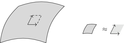
Figure 13. Linear Approximation

Thus it is reasonable to define the $m$-dimensional extent of $M$ by

$$\int_{M}|dx|_{M}=\int_{U}\sqrt{\det(\partial_{i}\phi|\partial_{j}\phi)}\,du$$

with $\sqrt{\det(\partial_{i}\phi|\partial_{j}\phi)}$ called the extent density of $\phi$. Although this definition is fairly speculative but it bears several desirable properties:

1. It correctly responds under scaling: For $r>0$, $rM$ is parametrized by $r\phi$ and $\sqrt{\det(\partial_{i}r\phi|\partial_{j}r\phi)}=r^{m}\sqrt{\det(\partial_{i}\phi|\partial_{j}\phi)}$ shows

   $$\int_{U}\sqrt{\det\Bigl{(}\frac{\partial r\phi}{\partial u_{i}}\Bigl{|}\frac{\partial r\phi}{\partial u_{j}}\Bigr{.}\Bigr{)}}\,du=r^{m}\int_{U}\sqrt{\det\Bigl{(}\frac{\partial\phi}{\partial u_{i}}\Bigl{|}\frac{\partial\phi}{\partial u_{j}}\Bigr{.}\Bigr{)}}\,du.$$

2. It is invariant under Euclidean transformations in $\text{\ym R}^{d}$. Let $T:\text{\ym R}^{d}\to\text{\ym R}^{d}$ be a Euclidean transformation, then $TM$ is parametrized by $T\phi$ and $\det(\partial_{i}(T\phi)|\partial_{j}(T\phi))=\det(\partial_{i}\phi|\partial_{j}\phi)$ gives the invariance.

3. It is independent of choices of parametrization. In fact, for another parametrization $V\ni v\mapsto\psi(v)\in M$ of $M$ with $V$ an open subset of $\text{\ym R}^{m}$, the chain rule

   $$\Bigl{(}\frac{\partial\phi}{\partial u_{i}}\Bigl{|}\frac{\partial\phi}{\partial u_{j}}\Bigr{.}\Bigr{)}=\sum_{k,l}\Bigl{(}\frac{\partial\phi}{\partial v_{k}}\Bigl{|}\frac{\partial\phi}{\partial v_{l}}\Bigr{.}\Bigr{)}\frac{\partial v_{k}}{\partial u_{i}}\frac{\partial v_{l}}{\partial u_{j}}$$

   gives

   $$\sqrt{\det\Bigl{(}\frac{\partial\phi}{\partial u_{i}}\Bigl{|}\frac{\partial\phi}{\partial u_{j}}\Bigr{.}\Bigr{)}}=\sqrt{\det\Bigl{(}\frac{\partial\phi}{\partial v_{k}}\Bigl{|}\frac{\partial\phi}{\partial v_{l}}\Bigr{.}\Bigr{)}}\,\Bigl{|}\frac{dv}{du}\Bigr{|},$$

   whence

   $$\int_{U}\sqrt{\det\Bigl{(}\frac{\partial\phi}{\partial u_{i}}\Bigl{|}\frac{\partial\phi}{\partial u_{j}}\Bigr{.}\Bigr{)}}\,du=\int_{V}\sqrt{\det\Bigl{(}\frac{\partial\phi}{\partial v_{k}}\Bigl{|}\frac{\partial\phi}{\partial v_{l}}\Bigr{.}\Bigr{)}}\,dv.$$

Definition 8.1.

The last property of extent density allows us to define the surface integral of a function $f$ on $M\subset\text{\ym R}^{d}$ in a coordinate-free fashion:

$$\int_{M}f(x)\,|dx|_{M}=\int_{U}f(\phi(u))\sqrt{\det\Bigl{(}\frac{\partial\phi}{\partial u_{i}}\Bigl{|}\frac{\partial\phi}{\partial u_{j}}\Bigr{.}\Bigr{)}}\,du,$$

where the notation indicates that it is based on a measure $|\cdot|_{M}$ in $M$.

Let $I_{\phi}$ be a preintegral on $C_{c}(U)$ defined by

$$I_{\phi}(g)=\int_{U}g(u)\sqrt{\det\Bigl{(}\frac{\partial\phi}{\partial u_{i}}\Bigl{|}\frac{\partial\phi}{\partial u_{j}}\Bigr{.}\Bigr{)}}\,du$$

with its Daniell extension denoted by $I_{\phi}^{1}:L^{1}(U,\phi)\to\text{\ym R}$.

Since parametrization-independence in the surface integral is based on the Jacobian formula, the integrability of a function on $M$ (surface-integrability) has a meaning and the set $L^{1}(M)$ of surface-integrable functions turns out to be a linear lattice isomorphic to $L^{1}(U,\phi)$.

Example 8.2.

1. For a smooth curve $C\subset\text{\ym R}^{d}$ parametrized by $x=\phi(t)$ ($a<t<b$) with $m=1$,

   $$\int_{C}|dx|_{C}=\int_{a}^{b}\left|\frac{d\phi}{dt}\right|\,dt$$

   is the length of $C$.

2. For a smooth surface $M\subset\text{\ym R}^{d}$ parametrized by $x=\phi(s,t)$ with $(s,t)\in U\subset\text{\ym R}^{2}$,

   $$\int_{M}|dx|_{M}=\int_{U}\sqrt{\Bigl{(}\frac{\partial\phi}{\partial s}\Bigl{|}\frac{\partial\phi}{\partial s}\Bigr{.}\Bigr{)}\Bigl{(}\frac{\partial\phi}{\partial t}\Bigl{|}\frac{\partial\phi}{\partial t}\Bigr{.}\Bigr{)}-\Bigl{(}\frac{\partial\phi}{\partial s}\Bigl{|}\frac{\partial\phi}{\partial t}\Bigr{.}\Bigr{)}^{2}}\,dsdt.$$

   When $d=3$ and $\phi$ is denoted by $\phi(s,t)=(x(s,t),y(s,t),z(s,t))$, the extent density takes the form

   $$\Bigl{|}\frac{\partial\phi}{\partial s}\times\frac{\partial\phi}{\partial t}\Bigr{|}=\\ \sqrt{\Bigl{(}\frac{\partial y}{\partial s}\frac{\partial z}{\partial t}-\frac{\partial z}{\partial s}\frac{\partial y}{\partial t}\Bigr{)}^{2}+\Bigl{(}\frac{\partial z}{\partial s}\frac{\partial x}{\partial t}-\frac{\partial x}{\partial s}\frac{\partial z}{\partial t}\Bigr{)}^{2}+\Bigl{(}\frac{\partial x}{\partial s}\frac{\partial y}{\partial t}-\frac{\partial y}{\partial s}\frac{\partial x}{\partial t}\Bigr{)}^{2}}.$$

3. Let $\varphi$ be a continuously differentiable function of $u\in U$ with $U$ an open subset of $\text{\ym R}^{d}$ and consider a $d$-dimesional surface $M=\{(\varphi(u),u);u\in U\}$ in $\text{\ym R}^{d+1}$ with $\phi(u)=(\varphi(u),u)$. Then

   $$\det(\partial_{j}\phi|\partial_{k}\phi)=\det(\phi^{\prime}){}^{t}(\phi^{\prime})=1+|\varphi^{\prime}|^{2}$$

   by the Cauchy-Binet formula in Appendix D (or by a simple computation with rank-one operators) and the surface integral on $M$ is described by

   $$\int_{M}f(x)\,|dx|_{M}=\int_{U}f(\varphi(u),u))\sqrt{1+|\varphi^{\prime}(u)|^{2}}\,du.$$

Example 8.3.

Consider a circle $(x-a)^{2}+z^{2}=b^{2}$ ($0<b<a$) in the $xz$-plane and rotate it around the $z$-axis to get a torus $(\sqrt{x^{2}+y^{2}}-a)^{2}+z^{2}=b^{2}$. To compute the surface area, we parametrize its upper half by

$$x=(a+b\sin\theta)\cos\varphi,\quad y=(a+b\sin\theta)\sin\varphi,\quad z=b\cos\theta$$

with

$$0\leq\varphi\leq 2\pi,\quad-\frac{\pi}{2}\leq\theta\leq\frac{\pi}{2}.$$

Then

$$\frac{\partial(x,y,z)}{\partial(\varphi,\theta)}=\begin{pmatrix}-(a+b\sin\theta)\sin\varphi&b\cos\theta\cos\varphi\\ (a+b\sin\theta)\cos\varphi&b\cos\theta\sin\varphi\\ 0&-b\sin\theta\\ \end{pmatrix}$$

and

$${\rule{0.0pt}{14.22636pt}}^{t}\left(\frac{\partial(x,y,z)}{\partial(\varphi,\theta)}\right)\left(\frac{\partial(x,y,z)}{\partial(\varphi,\theta)}\right)=\begin{pmatrix}(a+b\sin\theta)^{2}&0\\ 0&b^{2}\end{pmatrix}$$

shows that the density is $b(a+b\sin\theta)$. Thus the toral surface area is

$$2b\int_{-\pi/2}^{\pi/2}(a+b\sin\theta)\,d\theta\int_{0}^{2\pi}d\varphi=2\pi a2\pi b.$$

Exercise 35.

Compute the length of the coil $C\subset\text{\ym R}^{3}$: $\phi(t)=(a\cos t,b\sin t,bt)$ ($0\leq t\leq\tau$).

Exercise 36.

The $(d-1)$-dimensional extent of the simplex $M=\{x\in\text{\ym R}^{d};x_{1}\geq 0,\dots,x_{d}\geq 0,x_{1}+\dots+x_{d}=1\}$ in $\text{\ym R}^{d}$ is $\sqrt{d}/(d-1)!$.

Exercise 37.

Assume that $\phi:U\to M\subset\text{\ym R}^{d}$ is a product of an $m^{\prime}$-dimensional parametrization $\varphi:U^{\prime}\to M^{\prime}\subset\text{\ym R}^{d^{\prime}}$ and an $m^{\prime\prime}$-dimensional parametrization $\psi:U^{\prime\prime}\to M^{\prime\prime}\subset\text{\ym R}^{d^{\prime\prime}}$, i.e., $U=U^{\prime}\times U^{\prime\prime}$, $M=M^{\prime}\times M^{\prime\prime}$ and $\phi(u)=(\varphi(u^{\prime}),\psi(u^{\prime\prime}))$ for $u=(u^{\prime},u^{\prime\prime})\in\text{\ym R}^{m^{\prime}}\times\text{\ym R}^{m^{\prime\prime}}$.

Then $\int_{M}|dx|_{M}=\int_{M^{\prime}}|dx^{\prime}|_{M^{\prime}}\,\int_{M^{\prime\prime}}|dx^{\prime\prime}|_{M^{\prime\prime}}$ with $(x^{\prime},x^{\prime\prime})\in\text{\ym R}^{d^{\prime}}\times\text{\ym R}^{d^{\prime\prime}}$.

Remark 10.

Intuitively, a single coordinate parametrization is enough to almost cover $M$ by removing lower dimensional negligible parts.

We shall now extend the construction so far for a single coordinate parametrization to the case of multiple parametrization where $M$ is described by a family of coordinate parametrizations.

Assume that we are given a family of continuously differentiable one-to-one maps $\phi_{\alpha}:U_{\alpha}\to\text{\ym R}^{d}$ ($U_{\alpha}$ being an open subset of $\text{\ym R}^{m}$) so that (i) $\text{rank}(\phi_{\alpha}^{\prime}(u):\text{\ym R}^{m}\to\text{\ym R}^{d})=m$ for $u\in U_{\alpha}$, (ii) $M=\bigcup_{\alpha}\phi_{\alpha}(U_{\alpha})$ and (iii), if $\phi_{\alpha}(U_{\alpha})\cap\phi_{\beta}(U_{\beta})\not=\emptyset$, the bijection $\phi_{\beta}^{-1}\phi_{\alpha}:\phi_{\alpha}^{-1}(\phi_{\beta}(U_{\beta}))\to\phi_{\beta}^{-1}(\phi_{\alpha}(U_{\alpha}))$ defined by $\phi_{\alpha}(u)=\phi_{\beta}((\phi_{\beta}^{-1}\phi_{\alpha})(u))$ ($u\in\phi_{\alpha}^{-1}(\phi_{\beta}(U_{\beta}))$) is continuously differentiable. (The geomtric object $M\subset\text{\ym R}^{d}$ is a so-called immersed submanifold.)

A one-to-one map $\varphi$ of an open subset $U$ of $\text{\ym R}^{m}$ into $M$ is then called a coordinate chart of $M$ if both $\varphi^{-1}(\phi_{\alpha}(U_{\alpha}))=\{u\in U;\varphi(u)\in\phi_{\alpha}(U_{\alpha})\}$ and $\phi_{\alpha}^{-1}(\varphi(U))=\{u\in U_{\alpha};\phi_{\alpha}(u)\in\varphi(U)\}$ are open in $\text{\ym R}^{m}$ with the associated bijection $\phi_{\alpha}^{-1}\varphi:\varphi^{-1}(\phi_{\alpha}(U_{\alpha}))\to\phi_{\alpha}^{-1}(\varphi(U))$ as well as its inverse map continuously differentiable for each $\phi_{\alpha}:U_{\alpha}\to\text{\ym R}^{d}$. Here $\phi_{\alpha}^{-1}\varphi$ is defined by $\phi_{\alpha}((\phi_{\alpha}^{-1}\varphi)(u))=\varphi(u)$ ($u\in\varphi^{-1}(\phi_{\alpha}(U_{\alpha}))$).

Thus each map $U_{\alpha}\ni u\mapsto\phi_{\alpha}(u)\in M$ is a coordinate chart and, if $\psi:V\to M$ is another coordinate chart, the coordinate transformation $\psi^{-1}\varphi:\varphi^{-1}(\psi(V))\ni u\mapsto v\in\psi^{-1}(\varphi(U))$ defined by $\varphi(u)=\psi(v)$ is a continuously differentiable bijection from an open set $\varphi^{-1}(\psi(V))$ in $\text{\ym R}^{m}$ onto another open set $\psi^{-1}(\varphi(U))$ in $\text{\ym R}^{m}$.

Figure 14. Coordinate Transformation

Since open sets are Lebesgue measurable, so are their cuts and unions. Moreover Lebesgue measurable sets are preserved under coordinate transformations (Proposition 7.8), which enables us to cut and union $L^{1}(U,\varphi)$ for various coordinate charts $\varphi:U\to M$ to obtain a single space $L^{1}(M)$: The detailed construction is as follows.

Consider a function $f$ on $M$ which admits a finitely many coordinate charts $(\phi_{\alpha}:U_{\alpha}\to M\subset\text{\ym R}^{d})$ satisfying $\phi_{\alpha}(U_{\alpha})f\in L^{1}(\phi_{\alpha}(U_{\alpha}))$ for each $\alpha$ and $(\bigcup_{\alpha}\phi_{\alpha}(U_{\alpha}))f=f$.

Lemma 8.4.

1. We can find measurable sets $A_{\alpha}\subset U_{\alpha}$ so that $\bigcup_{\alpha}\phi_{\alpha}(U_{\alpha})=\bigsqcup\phi_{\alpha}(A_{\alpha})$ (a disjoint union).

2. Let $\phi:U\to\bigcup_{\alpha}\phi_{\alpha}(U_{\alpha})\subset\text{\ym R}^{d}$ be a coordinate chart of $M$. Then $\phi(U)f\in L^{1}(\phi(U))$.

Proof.

(i) Write $\alpha=1,2,\dots,l$ and let $A_{\alpha}$ be defined by

$$A_{\alpha} =\phi_{\alpha}^{-1}\Bigl{(}\bigl{(}\phi_{1}(U_{1})\cup\dots\cup\phi_{\alpha}(U_{\alpha})\bigr{)}\setminus\bigl{(}(\phi_{1}(U_{1})\cup\dots\cup\phi_{\alpha-1}(U_{\alpha-1})\bigr{)}\Bigr{)}$$

$$=\phi_{\alpha}^{-1}\Bigl{(}\phi_{\alpha}(U_{\alpha})\setminus\bigl{(}(\phi_{1}(U_{1})\cup\dots\cup\phi_{\alpha-1}(U_{\alpha-1})\bigr{)}\Bigr{)}$$

$$=U_{\alpha}\setminus\phi_{\alpha}^{-1}\bigl{(}(\phi_{1}(U_{1})\cup\dots\cup\phi_{\alpha-1}(U_{\alpha-1})\bigr{)},$$

which is Lebesgue measurable as a difference of open subsets.

(ii) Since $U_{\alpha}\cap\phi_{\alpha}^{-1}\phi(U)$ is Lebesgue measurable as an open subset, so is $A_{\alpha}\cap\phi_{\alpha}^{-1}\phi(U)$, whence $A_{\alpha}\cap\phi_{\alpha}^{-1}\phi(U)(f\circ\phi_{\alpha})\sqrt{\det(\partial_{i}\phi_{\alpha}|\partial_{j}\phi)}$ belongs to $L^{1}(U_{\alpha})$ as a cut of $(f\circ\phi_{\alpha})\sqrt{\det(\partial_{i}\phi_{\alpha}|\partial_{j}\phi_{\alpha})}$ by a Lebesgue measurable set and then, by the Jacobian formula applied to $\phi^{-1}\phi_{\alpha}:U_{\alpha}\cap\phi_{\alpha}^{-1}\phi(U)\to U\cap\phi^{-1}\phi_{\alpha}(U_{\alpha})$, $(U\cap\phi^{-1}\phi_{\alpha}(A_{\alpha}))(f\circ\phi)$ is Lebesgue integrable for each $\alpha$. Consequently

$$U(f\circ\phi)\sqrt{\det(\partial_{i}\phi|\partial_{j}\phi)}=\sum_{\alpha}(U\cap\phi^{-1}\phi_{\alpha}(A_{\alpha}))(f\circ\phi)\sqrt{\det(\partial_{i}\phi|\partial_{j}\phi)}$$

belongs to $L^{1}(U)$, i.e., $\phi(U)f\in L^{1}(\phi(U))$. ∎

Let $L(M)$ be the totality of functions considered so far. Clearly $L(M)$ is closed under lattice operations and in fact a linear lattice in view of the above lemma.

Exercise 38.

Show that $L(M)$ is a linear space.

For $f\in L(M)$, choose $\varphi_{\alpha}:U_{\alpha}\to M$ as before and measurable sets $A_{\alpha}\subset U_{\alpha}$ so that $\bigcup_{\alpha}\varphi_{\alpha}(U_{\alpha})=\bigsqcup_{\alpha}\varphi_{\alpha}(A_{\alpha})$ (Lemma 8.4 (i)). A linear functional $I(f)$ of $f\in L(M)$ is then well-defined by

$$I(f)=\sum_{\alpha}I_{\varphi_{\alpha}}(A_{\alpha}(f\circ\varphi_{\alpha})).$$

In fact, for another choice $\psi_{\beta}:V_{\beta}\to M$ with $B_{\beta}\subset V_{\beta}$ covering $f$,

$$\sum_{\alpha}I_{\varphi_{\alpha}}(A_{\alpha}(f\circ\varphi_{\alpha})) =\sum_{\alpha,\beta}I_{\varphi_{\alpha}}((A_{\alpha}\cap\varphi_{\alpha}^{-1}(\psi_{\beta}(B_{\beta})))(f\circ\varphi_{\alpha}))$$

$$=\sum_{\alpha,\beta}I_{\psi_{\beta}}((\psi_{\beta}^{-1}(\varphi_{\alpha}(A_{\alpha}))\cap B_{\beta})(f\circ\psi_{\beta}))$$

$$=\sum_{\beta}I_{\psi_{\beta}}(B_{\beta}(f\circ\psi_{\beta})).$$

The linear functional $I(f)$ is a preintegral because $f_{n}\downarrow 0$ for $f_{n}\in L(M)$ implies

$$\lim_{n\to\infty}I(f_{n})=\lim_{n\to\infty}\sum_{\alpha}I_{\varphi_{\alpha}}(A_{\alpha}(f_{n}\circ\varphi_{\alpha}))=\sum_{\alpha}\lim_{n\to\infty}I_{\varphi_{\alpha}}(A_{\alpha}(f_{n}\circ\varphi_{\alpha}))=0.$$

Let $I^{1}:L^{1}(M)\to\text{\ym R}$ be the Daniell extension of $I$ on $L(M)$, which contains $L^{1}(\varphi(U))$ as a linear sublattice for each coordinate chart $\varphi:U\to M$ in such a way that $I^{1}(f)=I_{\varphi}^{1}(f\circ\varphi)$ ($f\in L^{1}(\varphi(U))$) with $I^{1}(f)$ reasonably denoted by

$$\int_{M}f(x)\,|dx|_{M}.$$

Exercise 39.

Let $M\subset\text{\ym R}^{d}$ be the product of $M^{\prime}\subset\text{\ym R}^{d^{\prime}}$ and $M^{\prime\prime}\subset\text{\ym R}^{d^{\prime\prime}}$. Then, for $f\in C_{c}(M)$, functions

$$x^{\prime}\mapsto\int_{M^{\prime\prime}}f(x^{\prime},x^{\prime\prime})\,|dx^{\prime\prime}|_{M^{\prime\prime}},\quad x^{\prime\prime}\mapsto\int_{M^{\prime}}f(x^{\prime},x^{\prime\prime})\,|dx^{\prime}|_{M^{\prime}}$$

belong to $C_{c}(M^{\prime})$ and $C_{c}(M^{\prime\prime})$ respectively for which the repeated integral formula holds:

$$\int_{M}f(x)\,|dx|_{M}=\int_{M^{\prime}}|dx^{\prime}|_{M^{\prime}}\int_{M^{\prime\prime}}f(x^{\prime},x^{\prime\prime})\,|dx^{\prime\prime}|_{M^{\prime\prime}}.$$

Density formula: The following is known as a smooth version of the coarea formula in geometric measure theory.

Let $\psi:D\ni x\mapsto v\in\text{\ym R}^{n}$ ($D\subset\text{\ym R}^{d}$ being an open set) be a submersion and $M$ be a level set $[\psi=v]$ of $\psi$ at $v\in\text{\ym R}^{n}$. Let $f\in C_{c}(D)$ be localized in a neighborhood of a point $a\in M\subset\text{\ym R}^{d}$. Thanks to the inverse mapping theorem, after a suitable permutation of coordinates of $x$, we may assume that $x\mapsto(u,v)$ with $u=(x_{1},\dots,x_{m})$ and $v=\psi(x)$ is a local diffeomorphism in a neighborhood of $a$ ($m+n=d$). Here diffeomorphism is synonymous with smooth change-of-variables.

Then the inverse diffeomorphism is of the form $(u,v)\mapsto x=(u,\varphi(u,v))$ and their differentials are given by

$$\frac{\partial x}{\partial(u,v)}=\begin{pmatrix}1_{m}&0\\ \frac{\partial\varphi}{\partial u}&\frac{\partial\varphi}{\partial v}\end{pmatrix},\quad\frac{\partial(u,v)}{\partial x}=\begin{pmatrix}1&&0&0&\dots&0\\ &\ddots&&\vdots&\ddots&\vdots\\ 0&&1&0&\dots&0\\ \frac{\partial v}{\partial x_{1}}&\dots&\frac{\partial v}{\partial x_{m}}&\frac{\partial v}{\partial x_{m+1}}&\dots&\frac{\partial v}{\partial x_{m+n}}\end{pmatrix}.$$

Since these are inverses of each other, we have

$$\frac{\partial\varphi}{\partial v}\begin{pmatrix}\frac{\partial v}{\partial x_{m+1}}&\dots&\frac{\partial v}{\partial x_{m+n}}\end{pmatrix}=1_{n},\quad\frac{\partial\varphi}{\partial u}+\frac{\partial\varphi}{\partial v}\begin{pmatrix}\frac{\partial v}{\partial x_{1}}&\dots&\frac{\partial v}{\partial x_{m}}\end{pmatrix}=0.$$

Here $1_{m}$ and $1_{n}$ denote identity matrices of size $m$ and $n$ respectively.

As a local parametrization of level sets $[\psi=v]\subset\text{\ym R}^{d}$ ($v$ moving in a small open subset $V\subset\text{\ym R}^{n}$), we can take one of the form $U\ni u\mapsto x=(u,\varphi(u,v))\in\text{\ym R}^{d}$ (with $U$ a neighborhood of $a\in\text{\ym R}^{m}$ and $\varphi(u,v)$ a continuously differentiable function of $(u,v)$) so that the extent density is given by

$$\sqrt{\det\bigl{(}\delta_{i,j}+(\partial_{i}\varphi|\partial_{j}\varphi)\bigr{)}},\quad\partial_{i}\varphi=\frac{\partial\varphi}{\partial u_{i}}(u,v)$$

and the surface integral of $f$ on $[\psi=v]\subset D$ by

$$\int_{[\psi=v]}f(x)\,|dx|_{[\psi=v]}=\int_{U}f(u,\varphi(u,v))\sqrt{\det\bigl{(}\delta_{i,j}+(\partial_{i}\varphi|\partial_{j}\varphi)\bigr{)}}\,du.$$

Lemma 8.5.

Let $A$ be an $m\times m$ invertible matrix, $C$ be an $n\times n$ invertible matrix and $B$ be an $n\times m$ matrix. We set $G=-C^{-1}BA^{-1}$ so that

$$\begin{pmatrix}A&0\\ B&C\end{pmatrix}^{-1}=\begin{pmatrix}A^{-1}&0\\ G&C^{-1}\end{pmatrix}.$$

Then

$$\det(A)^{-2}\det({}^{t}AA+{}^{t}BB)=\det(C)^{2}\det(G\,{}^{t}G+C^{-1\,}{}^{t}C^{-1}).$$

Proof.

Just compute as follows:

$$\det(A)^{-2}\det({}^{t}AA+{}^{t}BB) =\det(1_{m}+{}^{t}(BA^{-1})(BA^{-1}))$$

$$=\det(1_{n}+(BA^{-1})\,{}^{t}(BA^{-1}))$$

$$=\det(1_{n}+(-CG)\,{}^{t}(-CG))$$

$$=\det(C)^{2}\det(G\,{}^{t}G+C^{-1\,}{}^{t}C^{-1}).$$

Here Sylvester’s formula (Appendix D) is used in the second line. ∎

We apply the above lemma for $A=1_{m}$, $B=\frac{\partial\varphi}{\partial u}$ and $C=\frac{\partial\varphi}{\partial v}$ with $(G\ C^{-1})=\frac{\partial\psi}{\partial x}$ to get

$$\det\Bigl{(}\delta_{i,j}+\bigl{(}\frac{\partial\varphi}{\partial u_{i}}|\frac{\partial\varphi}{\partial u_{j}}\bigr{)}\Bigr{)}=\det\Bigl{(}\frac{\partial\varphi}{\partial v}\Bigr{)}^{2}\det(\psi_{\imath}^{\prime}|\psi_{\jmath}^{\prime}),\quad(\psi_{\imath}^{\prime}|\psi_{\jmath}^{\prime})=\sum_{k=1}^{d}\frac{\partial\psi_{\imath}}{\partial x_{k}}\frac{\partial\psi_{\jmath}}{\partial x_{k}},$$

which is used to see

$$\int_{\psi^{-1}(V)}f(x) \sqrt{\det(\psi_{\imath}^{\prime}|\psi_{\jmath}^{\prime})}\,dx$$

$$=\int_{U\times V}f(u,\varphi(u,v))\sqrt{\det(\psi_{\imath}^{\prime}|\psi_{\jmath}^{\prime})}\Bigl{|}\det\Bigl{(}\frac{\partial x}{\partial(u,v)}\Bigr{)}\Bigr{|}\,dudv$$

$$=\int_{U\times V}f(u,\varphi(u,v))\sqrt{\det(\psi_{\imath}^{\prime}|\psi_{\jmath}^{\prime})}\Bigl{|}\det\Bigl{(}\frac{\partial\varphi}{\partial v}\Bigr{)}\Bigr{|}\,dudv$$

$$=\int_{V}dv\,\int_{U}f(u,\varphi(u,v))\sqrt{\det\Bigl{(}\delta_{i,j}+\bigl{(}\frac{\partial\varphi}{\partial u_{i}}|\frac{\partial\varphi}{\partial u_{j}}\bigr{)}\Bigr{)}}\,du$$

$$=\int_{V}dv\,\int_{[\psi=v]}f(x)\,|dx|_{[\psi=v]}.$$

Finally this localized identity is patched up globally, this time by a partition of unity (Proposition 4.22), to have the following.

Theorem 8.6.

Given a submersion $\psi:\text{\ym R}^{d}\supset D\ni x\mapsto\psi(x)\in\text{\ym R}^{n}$ and a function $f\in C_{c}(D)$, we have

$$\int_{D}f(x)\sqrt{\det(\psi_{\imath}^{\prime}|\psi_{\jmath}^{\prime})}\,dx=\int_{\psi(D)}dv\,\int_{[\psi=v]}f(x)\,|dx|_{[\psi=v]}.$$

Proof.

By the local formula, each point $a\in[f]$ has an open neighborhood $W$ such that the global forumla holds if $f$ belongs to $C_{c}(W)\subset C_{c}(D)$. From the finite covering property, we can find a finitely many such open sets $W_{\alpha}$ so that $[f]\subset\bigcup W_{\alpha}$. We apply the partition of unity to this covering to get $h_{\alpha}\in C_{c}(W_{\alpha})$ satisfying $\sum_{\alpha}h_{\alpha}=1$ on $[f]$.

Then $f_{\alpha}=h_{\alpha}f\in C_{c}(W_{\alpha})$ is summed to be $f$ and we have

$$\int_{D}f(x)\sqrt{\det(\psi_{\imath}^{\prime}|\psi_{\jmath}^{\prime})}\,dx =\sum_{\alpha}\int_{D}f_{\alpha}(x)\sqrt{\det(\psi_{\imath}^{\prime}|\psi_{\jmath}^{\prime})}\,dx$$

$$=\sum_{\alpha}\int_{\psi(D)}dv\,\int_{[\psi=v]}f_{\alpha}(x)\,|dx|_{[\psi=v]}$$

$$=\int_{\psi(D)}dv\,\int_{[\psi=v]}f(x)\,|dx|_{[\psi=v]}.$$

∎

Corollary 8.7.

Let $M=[\psi=v]$ be a level set of $\psi$. Then

$$\lim_{V\to v}\frac{1}{|V|}\int_{\psi^{-1}(V)}f(x)\sqrt{\det(\psi_{\imath}^{\prime}|\psi_{\jmath}^{\prime})}\,dx=\int_{M}f(x)\,|dx|_{M}.$$

Remark 11.

By rewriting surface integrals in terms of Hausdorff measure, a further generalization is known as the coarea formula in geometric measure theory (see [1]).

Example 8.8.

Let $\psi:D=\text{\ym R}^{d}\to\text{\ym R}^{n}$ be a linear map, which is identified with an $n\times d$ matrix, and assume that the cut of $\psi$ by the last $n$ columns is invertible as an $n\times n$ matrix. Then local coordinates $(u,v)\in\text{\ym R}^{m+n}$ satisfying

$$\begin{pmatrix}u\\ v\end{pmatrix}=\left(\begin{array}[]{c c}I_{m}&0\\ \lx@intercol\hfil\psi\hfil\lx@intercol\end{array}\right)x\iff x=\begin{pmatrix}I_{m}&0\\ B&C\end{pmatrix}\begin{pmatrix}u\\ v\end{pmatrix}\ \text{with}\ \varphi(u,v)=Bu+Cv$$

provides global one and the equality of

$$\int_{D}f(x)\sqrt{\det((\psi_{i}^{\prime}|\psi_{j}^{\prime}))}\,dx=\int_{\text{\ym R}^{d}}f(x)\sqrt{\det(\psi{}^{t}\psi)}\,dx$$

and

$$\int_{\psi(D)}dv\int_{[\psi=v]}F(x)\,|dx|_{[\psi=v]}=\int_{\text{\ym R}^{n}}dv\int_{\text{\ym R}^{m}}f(u,\varphi(u,v))|\det(C)|\sqrt{\det(\psi{}^{t}\psi)}\,du$$

is reduced to the identity

$$\int_{\text{\ym R}^{d}}f(x)\,dx=|\det(C)|\int_{\text{\ym R}^{n}}dv\int_{\text{\ym R}^{m}}f(u,\varphi(u,v))\,du,$$

which is nothing but a combination of the (linear) Jacobian formula and repeated integrals.

Example 8.9.

Let $\psi(x)=|x|$ for $0\not=x\in\text{\ym R}^{d}$ ($D=\text{\ym R}^{d}\setminus\{0\}$, $n=1$). Then $\psi^{\prime}(x)=\frac{x}{|x|}$ and

$$\int_{D}f(x)\,dx =\int_{0}^{\infty}dr\int_{rS^{d-1}}f(x)\,|dx|_{rS^{d-1}}$$

$$=\int_{0}^{\infty}dr\,r^{d-1}\int_{S^{d-1}}f(r\omega)\,|d\omega|_{S^{d-1}}.$$

Now, for the choice $f(x)=e^{-|x|^{2}}$,

$$\int_{\text{\ym R}^{d}}e^{-|x|^{2}}\,dx=\int_{D}e^{-|x|^{2}}\,dx=|S^{d-1}|\int_{0}^{\infty}r^{d-1}e^{-r^{2}}\,dr.$$

The left hand side is equal to $\pi^{d/2}$ as a multiple Gaussian integral and the integral in the right hand side is expressed in terms of the gamma function by $\Gamma(d/2)/2$, resulting in the spherical integral

$$|S^{d-1}|=\frac{2\pi^{d/2}}{\Gamma(d/2)}.$$

With this formula in hand, $f(x)=e^{-|x|^{\beta}}/|x|^{\alpha}$ for $\alpha\in\text{\ym R}$ and $\beta>0$ is then calculated as follows:

$$\int_{\text{\ym R}^{d}}\frac{e^{-|x|^{\beta}}}{|x|^{\alpha}}\,dx=|S^{d-1}|\int_{0}^{\infty}r^{d-1}\frac{e^{-r^{\beta}}}{r^{\alpha}}\,dr =|S^{d-1}|\frac{1}{\beta}\int_{0}^{\infty}s^{-1+(d-\alpha)/\beta}e^{-s}\,dt$$

$$=\begin{cases}\frac{2\pi^{d/2}}{\beta\Gamma(d/2)}\Gamma(\frac{d-\alpha}{\beta})&(\alpha<d),\\ \infty&(\alpha\geq d).\end{cases}$$

Exercise 40.

Check that $|S^{0}|=2$, $|S^{1}|=2\pi$ and $|S^{2}|=4\pi$.

Remark 12.

Square-rooted determinant densities are closely related to the Jacobian. To see this, consider a smooth map $\varphi:U\to\text{\ym R}^{n}$ defined on an open set $U\subset\text{\ym R}^{m}$ with $\varphi^{\prime}(x)$ a matrix-valued function of size $n\times m$. Then $\det(\partial_{i}\varphi|\partial_{j}\phi)=\det({}^{t}\varphi^{\prime}(x)\varphi^{\prime}(x))$ and $\det(\varphi_{i}^{\prime}(x)|\varphi_{j}^{\prime}(x))=\det(\varphi^{\prime}(x)\,{}^{t}\varphi^{\prime}(x))$, whence these coinside by Sylvester’s formula (Appendix D).

When $m=n$, they are reduced to $\det(\varphi^{\prime}(x))^{2}$. In accordance with this fact, their square roots are also called the Jacobian of $\varphi$.

We here restrict ourselves to the case $n=1$; $\psi$ is a scalar function and the level set $[\psi=v]$ is a hypersurface in $\text{\ym R}^{d}$. In the local coordinate expression

$$\int_{[\psi=v]}f(x)\,|dx|_{\psi=v}=\int_{U}f(x)\left|\frac{\partial\varphi}{\partial v}\right||\psi^{\prime}(x)|\,du\quad(x=(u,\varphi(u,v))),$$

notice that the density function is equal to the norm of a vector

$$(-\frac{\partial\varphi}{\partial u},1)=\frac{\partial\varphi}{\partial v}\psi^{\prime}=\frac{1}{\frac{\partial\psi}{\partial x_{d}}}\psi^{\prime},$$

which is normal to the hypersurface $[\psi=v]$ at the point $x=(u,\varphi(u,v))\in[\psi=v]$. In terms of the normal unit vector

$$\bm{n}(x)=\frac{1}{|\psi^{\prime}(x)|}\psi^{\prime}(x)$$

pointing to the direction of increasing $\psi$, we introduce a vector-valued measure (so-called surface element) by

$$dx_{[\psi=v]}=\bm{n}(x)|dx|_{[\psi=v]}$$

and, for a continuous vector field $F(x)\in\text{\ym R}^{d}$ ($x\in D$) of compact support, define the surface integral of $F$ on the hypersurface $[\psi=v]$ by

$$\int_{[\psi=v]}F(x)\cdot dx_{[\psi=v]}=\int_{[\psi=v]}F(x)\cdot\bm{n}(x)\,|dx|_{[\psi=v]}.$$

In local coordinates,

$$\bm{n}(x)=\frac{\epsilon}{\sqrt{1+|\partial\varphi/\partial u|^{2}}}\Bigl{(}-\frac{\partial\varphi}{\partial u},1\Bigr{)}\quad\text{with}\quad\epsilon=\frac{\partial\varphi}{\partial v}/\left|\frac{\partial\varphi}{\partial v}\right|\in\{\pm 1\}$$

and

$$\int_{[\psi=v]}F(x)\cdot dx_{[\psi=v]}=\int_{U}F(x)\cdot\psi^{\prime}(x)\left|\frac{\partial\varphi}{\partial v}\right|\,du\quad(x=(u,\varphi(u,v))).$$

When $F(x)=f(x)\bm{n}(x)$, this is reduced to the surface integral of the scalar function $f$.

Figure 15. Flux

Now assume that $F$ is continuously differentiable on $D$. If the compact support of $F$ is contained in an open set $W\subset\text{\ym R}^{d}$ for which $W\simeq U\times V$ by a local coordinate description of $\psi$ with $U\subset\text{\ym R}^{d-1}$ an open rectangle and $V\subset\text{\ym R}$ an open interval, we claim

$$\frac{d}{dv}\int_{[\psi=v]}F(x)\cdot dx_{[\psi=v]}=\int_{[\psi=v]}\frac{f(x)}{|\psi^{\prime}(x)|}\,|dx|_{[\psi=v]}.$$

Here $f$ is the divergence of $F$:

$$f(x)=\text{div}F=\sum_{i=1}^{d}\frac{\partial F_{i}}{\partial x_{i}}.$$

In fact, in local coordinates, the formula takes the form

$$\frac{d}{dv}\int_{U}\epsilon F\cdot(-\frac{\partial\varphi}{\partial u},1)\,du=\int_{U}\epsilon f(x)\frac{\partial\varphi}{\partial v}\,du\quad(x=(u,\varphi(u,v))).$$

From the chain rule relation

$$\frac{\partial}{\partial v}\left(F\cdot(-\frac{\partial\varphi}{\partial u},1)\right) =\frac{\partial}{\partial v}\left(-\sum_{i=1}^{d-1}F_{i}\frac{\partial\varphi}{\partial u_{i}}+F_{d}\right)$$

$$=-\sum_{i=1}^{d-1}\frac{\partial F_{i}}{\partial x_{d}}\frac{\partial\varphi}{\partial v}\frac{\partial\varphi}{\partial u_{i}}-\sum_{i=1}^{d-1}F_{i}\frac{\partial^{2}\varphi}{\partial v\partial u_{i}}+\frac{\partial F_{d}}{\partial x_{d}}\frac{\partial\varphi}{\partial v}$$

$$=-\sum_{i=1}^{d-1}\left(\frac{\partial F_{i}}{\partial x_{d}}\frac{\partial\varphi}{\partial v}\frac{\partial\varphi}{\partial u_{i}}+F_{i}\frac{\partial^{2}\varphi}{\partial v\partial u_{i}}+\frac{\partial F_{i}}{\partial x_{i}}\frac{\partial\varphi}{\partial v}\right)+f\frac{\partial\varphi}{\partial v}$$

$$=-\sum_{i=1}^{d-1}\frac{\partial}{\partial u_{i}}(F_{i}\frac{\partial\varphi}{\partial v})+f\frac{\partial\varphi}{\partial v},$$

the difference of the local formula therefore amounts to

$$\sum_{i=1}^{d-1}\int_{U}\frac{\partial}{\partial u_{i}}(F_{i}\frac{\partial\varphi}{\partial v})\,du,$$

which vanishes by repeated integral expressions in view of the fact that $F_{i}\frac{\partial\varphi}{\partial v}$ vanishes at the boundary of $U$:

$$\int_{U}\frac{\partial}{\partial u_{i}}(F_{i}\frac{\partial\varphi}{\partial v})\,du =\int_{U_{i}}(du)_{i}\int_{a_{i}}^{b_{i}}\frac{\partial}{\partial u_{i}}(F_{i}\frac{\partial\varphi}{\partial v})\,du_{i}$$

$$=\int_{U_{i}}\left(\left.F_{i}\frac{\partial\varphi}{\partial v}\right|_{u_{i}=b_{i}}-\left.F_{i}\frac{\partial\varphi}{\partial v}\right|_{u_{i}=a_{i}}\right)\,(du)_{i}=0.$$

Here $U=(a_{1},b_{1})\times\dots\times(a_{d-1},b_{d-1})$,

$$U_{i}=(a_{1},b_{1})\times\dots\times(a_{i-1},b_{i-1})\times(a_{i+1},b_{i+1})\times\dots\times(a_{d-1},b_{d-1})$$

and $(du)_{i}=du_{1}\cdots du_{i-1}du_{i+1}\cdots du_{d-1}$.

The local formula is now glued together by a partition of unity (cf. the proof of Theorem 8.6) to obtain the global formula.

Theorem 8.10.

Let $\psi:D\to\text{\ym R}$ be a submersion and $F\in C_{c}^{1}(D,\text{\ym R}^{d})$ be a continuously differentiable vector field of compact support on $D$. Then

$$\frac{d}{dv}\int_{[\psi=v]}F(x)\cdot dx_{[\psi=v]}=\int_{[\psi=v]}\frac{\text{div}\,F(x)}{|\psi^{\prime}(x)|}\,|dx|_{[\psi=v]}$$

for $v\in\psi(D)$.

Combined with the coarea formula (Theorem 8.6), we have the following.

Corollary 8.11 (Divergence Theorem).

Let $[a,b]\subset\psi(D)$. Then

$$\int_{[a\leq\psi\leq b]}\text{div}\,F(x)\,dx=\int_{[\psi=b]}F(x)\cdot dx_{[\psi=b]}-\int_{[\psi=a]}F(x)\cdot dx_{[\psi=a]}.$$

Figure 16. Flux Flow

As a limit case, consider the situation where $\psi(D)=(0,c)$ and $[\psi=v]$ approaches to a closed set $[\psi=0]$ as $v\to+0$ in such a way that $[\psi=0]\subset\partial D$, $[0\leq\psi<b]=[\psi=0]\sqcup[\psi<b]$ is an open set of $\text{\ym R}^{d}$ for any $0<b<c$ and

$$\lim_{v\to+0}\int_{[\psi=v]}f(x)\,|dx|_{[\psi=v]}=0\quad(f\in C_{c}^{+}([\psi\geq 0])).$$

The above flow version is then filled with the inner boundary $[\psi=0]$ to get the boundary version

$$\int_{[0\leq\psi<b]}\text{div}\,F(x)\,dx=\int_{[\psi=b]}F(x)\cdot dx_{\partial\widetilde{D}}\quad(F\in C_{c}^{1}([\psi\geq 0],\text{\ym R}^{d})).$$

Example 8.12 (Cylinder).

Let $x=(x^{\prime},x^{\prime\prime})\in\text{\ym R}^{d^{\prime}}\times\text{\ym R}^{d^{\prime\prime}}$ with $d^{\prime}+d^{\prime\prime}=d$, $D=\{x\in\text{\ym R}^{d};|x^{\prime}|>0\}$ and $\psi(x)=|x^{\prime}|$.

Then $\psi(D)=(0,\infty)$ and the inner boundary $[\psi=0]=\{0\}\times\text{\ym R}^{d^{\prime\prime}}$ fills up $D$ to get the whole space $\text{\ym R}^{d}$.

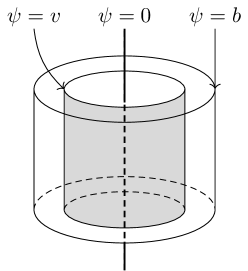
Figure 17. Cylinder

Example 8.13 (Sphere).

Let $\psi(x)=|x|$ and $D=\{x\in\text{\ym R}^{d};0<|x|\}$. Then $\bm{n}(x)=x/|x|$ ($x\in D$), $[\psi\geq 0]=\text{\ym R}^{d}$ and, for $F\in C_{c}^{1}(\text{\ym R}^{d},\text{\ym R}^{d})$,

$$\int_{[|x|<r]}\text{div}\,F(x)\,dx=\int_{[|x|=r]}\frac{F(x)\cdot x}{r}\,|dx|_{[|x|=r]}=r^{d-1}\int_{S^{d-1}}F(r\omega)\cdot\omega\,d\omega.$$

Exercise 41 (hydrostatic balance equation).

Let $D$ be a bounded open subset of $\text{\ym R}^{d}$ with a smooth boundary $\partial D$. Then

$$\int_{\partial D}dx_{\partial D}=0$$

as a vector in $\text{\ym R}^{d}$.

Exercise 42.

Show that, if $[0\leq\psi<b]$ is open for some $0<b<c$, then $[0\leq\psi<v]$ is open for any $v\geq b$.

9. Complex Functions

So far, we have dealt with real functions. For further applications in subjects such as Fourier analysis or quantum analysis, we should not avoid complex functions in values as well as in variables. Here the results established for real-valued functions are naturally extended to complex-valued functions.

Given a linear lattice $L$, we shall work with the complexified function space $L_{\text{\ym C}}=L+iL$, which is referred to as a complex lattice if the lattice condition is strengthened to $|f|\in L_{\text{\ym C}}$ ($f\in L_{\text{\ym C}}$), i.e. $\sqrt{f^{2}+g^{2}}\in L$ ($f,g\in L$). A linear functional $I:L\to\text{\ym R}$ is obviously extended to a complex-linear functional on $L_{\text{\ym C}}$, which is also denoted by $I$.

Here are some of simple facts on complex lattices.

Proposition 9.1.

Let $L_{\text{\ym C}}$ be a complex lattice.

1. Given a positive functional $I$ on $L$, the integral inequality $|I(f)|\leq I(|f|)$ ($f\in L_{\text{\ym C}}$) holds.

2. The complexification $L_{\uparrow}\cap L_{\downarrow}+iL_{\uparrow}\cap L_{\downarrow}$ of $L_{\uparrow}\cap L_{\downarrow}$ is also a complex lattice.

Proof.

(i) Since $I$ is real-valued on $L$, $\overline{I(f)}=I(\overline{f})$ for $f\in L_{\text{\ym C}}$. If $I(f)=0$, the integral inequality holds trivially. Otherwise the polar expression $I(f)=|I(f)|e^{i\theta}$ ($\theta\in\text{\ym R}$) is combined with $e^{-i\theta}f+e^{i\theta}\overline{f}\leq 2|f|$ to get

$$2|I(f)|=e^{-i\theta}I(f)+e^{i\theta}\overline{I(f)}=I(e^{-i\theta}f+e^{i\theta}\overline{f})\leq 2I(|f|).$$

(ii) In the expression $|f+ig|=\bigl{|}|f|+i|g|\bigr{|}$ ($f,g\in L_{\uparrow}\cap L_{\downarrow}$), we approximate $|f|,|g|\in L_{\uparrow}\cap L_{\downarrow}$ by sequences $\varphi^{\prime}_{n}$, $\varphi^{\prime\prime}_{n}$, $\psi^{\prime}_{n}$ and $\psi^{\prime\prime}_{n}$ in $L^{+}$ so that $\varphi_{n}^{\prime}\uparrow|f|$, $\varphi_{n}^{\prime\prime}\downarrow|f|$, $\psi_{n}^{\prime}\uparrow|g|$ and $\psi_{n}^{\prime\prime}\downarrow|g|$.

Then $|\varphi_{n}^{\prime}+i\psi_{n}^{\prime}|,|\varphi_{n}^{\prime\prime}+i\psi_{n}^{\prime\prime}|\in L$ satisfy

$$|\varphi_{n}^{\prime}+i\psi_{n}^{\prime}|\uparrow\bigl{|}|f|+i|g|\bigr{|},\quad|\varphi_{n}^{\prime\prime}+i\psi_{n}^{\prime\prime}|\downarrow\bigl{|}|f|+i|g|\bigr{|},$$

which implies $|f+ig|\in L_{\uparrow}\cap L_{\downarrow}$. ∎

Example 9.2.

The complexification $S_{\text{\ym C}}(\text{\ym R}^{d})=S(\text{\ym R}^{d})+iS(\text{\ym R}^{d})$ is a complex lattice and the volume integral on $S^{1}(\text{\ym R}^{d})$ is therefore complex-linearly extended to a functional $I:S_{\text{\ym C}}(\text{\ym R}^{d})\to\text{\ym C}$ and then further to

$$I_{\updownarrow}:S_{\uparrow}(\text{\ym R}^{d})\cap S_{\downarrow}(\text{\ym R}^{d})+iS_{\uparrow}(\text{\ym R}^{d})\cap S_{\downarrow}(\text{\ym R}^{d})\to\text{\ym C}$$

so that $|I_{\updownarrow}(f)|\leq I_{\updownarrow}(|f|)$ for $f\in S_{\uparrow}(\text{\ym R}^{d})\cap S_{\downarrow}(\text{\ym R}^{d})+iS_{\uparrow}(\text{\ym R}^{d})\cap S_{\downarrow}(\text{\ym R}^{d})$.

When $d=1$, definite and indefinite integrals as well as improper integrals are extended to complex-valued functions by replacing $S_{\uparrow}(\text{\ym R})\cap S_{\downarrow}(\text{\ym R})$ with its complexifications in such a way that the fundamental theorem of calculus remains valid.

Example 9.3.

For a complex parameter $c\not=0$,

$$\int e^{cx}\,dx=\frac{1}{c}e^{cx}.$$

For $c=-a-ib$ with $a>0$ and $b\in\text{\ym R}$, $e^{-(a+ib)t}=e^{-at}(\cos bt-i\sin bt)$ is integrable on $(0,\infty)$ and

$$\int_{0}^{\infty}e^{-(a+ib)t}\,dt=\frac{1}{a+ib}=\frac{a}{a^{2}+b^{2}}-i\frac{b}{a^{2}+b^{2}}.$$

Example 9.4.

Let $0\not=a\in\text{\ym C}$ have a non-negative real part. Then

$$\int_{-\infty}^{\infty}e^{-ax^{2}}\,dx=\sqrt{\frac{\pi}{a}},$$

where the complex root $\sqrt{a}$ is chosen so that $\sqrt{a}>0$ for $a>0$.

For the proof, see the compuation below.

As to the Daniell extension of a preintegral $I$ on a linear lattice $L$, the dominated convergence theorem as well as parametric differentiation holds for complex-valued functions. When $L_{\text{\ym C}}$ is a complex lattice, so is $L_{\text{\ym C}}^{1}=L^{1}+iL^{1}$ (Proposition B.7) but this is not obvious at all (see Appendix B for details).

For the volume integral in $\text{\ym R}^{d}$, however, it is practically enough to consider an open set $U\subset\text{\ym R}^{d}$ and the associated linear lattice $C(U)\cap L^{1}(U)$, for which $C(U)\cap L^{1}(U)+iC(U)\cap L^{1}(U)$ is a complex lattice.

Example 9.5.

The identity in Example 9.3 is differentiated repeatedly with respect to a complex parameter $c\in\text{\ym C}^{\times}$ to get

$$\int x^{n}e^{cx}\,dx=\frac{\partial^{n}}{(\partial c)^{n}}\left(\frac{1}{c}e^{cx}\right).$$

Example 9.6.

Example 9.4 is extended to

$$\int_{-\infty}^{\infty}e^{-ax^{2}+bx}\,dx=e^{b^{2}/4a}\sqrt{\frac{\pi}{a}}$$

for $b\in\text{\ym C}$. This is most simply related to Example 9.4 by Cauchy’s integral theorem but we here calculate as follows:

$$\sum_{n\geq 0}\frac{1}{n!}b^{n}\int_{-\infty}^{\infty}x^{n}e^{-ax^{2}}\,dx =\sum_{m\geq 0}\frac{1}{(2m)!}b^{2m}\int_{-\infty}^{\infty}x^{2m}e^{-ax^{2}}\,dx$$

$$=\sum_{m\geq 0}\frac{1}{(2m)!}b^{2m}\left(-\frac{\partial}{\partial a}\right)^{m}\int_{-\infty}^{\infty}e^{-ax^{2}}\,dx$$

$$=\sum_{m\geq 0}\frac{1}{(2m)!}b^{2m}\frac{(2m)!}{4^{m}m!}a^{-m-1/2}\pi^{1/2}$$

$$=e^{b^{2}/4a}\sqrt{\frac{\pi}{a}}.$$

For $f\in S_{\text{\ym C}}^{1}(\text{\ym R}^{d})=S^{1}(\text{\ym R}^{d})+iS^{1}(\text{\ym R}^{d})$ and $\xi\in\text{\ym R}^{d}$, $e^{-ix\xi}f(x)$ ($x\xi=x_{1}\xi_{1}+\dots+x_{d}\xi_{d}$) is integrable and the Fourier transform $\widehat{f}$ of $f$ is defined by

$${\widehat{f}}(\xi)=\int_{\text{\ym R}^{d}}f(x)e^{-ix\xi}\,dx,$$

which is a continuous function of $\xi\in\text{\ym R}^{d}$ by Proposition 4.17.

The Fourier transform is known to be isometric (called the Plancherel formula) in the sense that

$$\int_{\text{\ym R}^{d}}|\widehat{f}(\xi)|^{2}\,d\xi=(2\pi)^{d}\int_{\text{\ym R}^{d}}|f(x)|^{2}\,dx$$

for any integrable $f$ satisfying $\int|f(x)|^{2}\,dx<\infty$.

Example 9.7.

The Fourier transform of an interval $f=[-1,1]$ is

$$\widehat{f}(\xi)=2\frac{\sin\xi}{\xi}$$

with the Plancherel formula of the form $\int_{-\infty}^{\infty}(\sin\xi)^{2}/\xi^{2}\,d\xi=\pi$, which turns out to be the Dirichlet integral by Example 2.24.

Example 9.8.

The Fourier transform of $(0,\infty)e^{-rx}$ ($r>0$) is

$$\int_{0}^{\infty}e^{-rx}e^{-ix\xi}\,dx=\frac{1}{r+i\xi}.$$

Example 9.9.

For $0\not=a\in\text{\ym R}$, $0\not=b\in\text{\ym R}$ and $r>0$,

$$\int_{0}^{\infty}e^{-rt}\frac{e^{iat}-e^{ibt}}{t}\,dt=\log\frac{r-ib}{r-ia}.$$

Let $s\in\text{\ym R}$ and consider

$$f(s)=\int_{0}^{\infty}e^{-rt}\frac{e^{iast}-e^{ibst}}{t}\,dt$$

Then

$$f^{\prime}(s)=\int_{0}^{\infty}e^{-rt}(iae^{iast}-ibe^{ibst})\,dt=\frac{ia}{r-ias}-\frac{ib}{r-ibs}$$

is integrated to get

$$f(s)=\log(s-r/(ib))-\log(s-r/(ia))=\log\frac{r-ibs}{r-ias}.$$

Here the constant of integration is specified by the condition $f(0)=0$.

Example 9.10.

For $a>0$, $b>0$ and $r\geq 0$, the following holds.

$$\int_{0}^{\infty}e^{-rt}\frac{\cos(at)-\cos(bt)}{t}\,dt =\frac{1}{2}\log\frac{r^{2}+b^{2}}{r^{2}+a^{2}},$$

$$\int_{0}^{\infty}e^{-rt}\frac{b\sin(at)-a\sin(bt)}{t^{2}}\,dt =\frac{ab}{2}\int_{0}^{1}\log\frac{r^{2}+b^{2}u^{2}}{r^{2}+a^{2}u^{2}}\,du$$

with

$$\lim_{r\to+0}\int_{0}^{1}\log\frac{r^{2}+b^{2}u^{2}}{r^{2}+a^{2}u^{2}}\,du=2\log\frac{b}{a}.$$

The first equality for $r>0$ is just the real part of the formula in the previous example and the limit case $r=0$ is a consequence of Theorem 2.27 because $(\cos(at)-\cos(bt))/t$ is improperly integrable on $(0,\infty)$ in view of

$$\left(\frac{\sin(at)}{at}-\frac{\sin(bt)}{bt}\right)^{\prime}=\frac{\cos(at)-\cos(bt)}{t}-\frac{b\sin(at)-a\sin(bt)}{abt^{2}}.$$

To see the second equality, the function

$$g(s)=\int_{0}^{\infty}e^{-rt}\frac{b\sin(ast)-a\sin(bst)}{t^{2}}\,dt$$

of $s\in\text{\ym R}$ is differentiated to have

$$g^{\prime}(s)=ab\int_{0}^{\infty}e^{-rt}\frac{\cos(ast)-\cos(bst)}{t}\,dt=\frac{ab}{2}\log\frac{r^{2}+b^{2}s^{2}}{r^{2}+a^{2}s^{2}},$$

whence

$$g(s)=\frac{ab}{2}\int_{0}^{s}\log\frac{r^{2}+b^{2}u^{2}}{r^{2}+a^{2}u^{2}}\,du.$$

Finally, in view of $1\leq(r^{2}+b^{2}u^{2})/(r^{2}+a^{2}u^{2})\leq b^{2}/a^{2}$, the dominated convergence theorem is applied to get $\lim_{r\to+0}g(s)=sab\log(b/a)$.

Exercise 43.

1. With the help of $(u\log(r^{2}+a^{2}u^{2}))^{\prime}$, express the indefinite integral of $\log(r^{2}+a^{2}u^{2})$ by arctangent.

2. By integrating $\displaystyle\frac{d}{dt}\log(r^{2}+u^{2}t)$ from $t=a^{2}$ to $t=b^{2}$ and using repeated integrals, show that

   $$\lim_{r\to+0}\int_{0}^{1}\log\frac{r^{2}+b^{2}u^{2}}{r^{2}+a^{2}u^{2}}\,du=2\log\frac{b}{a}.$$

We shall evaluate Fresnel integrals by imitating Gaussian integrals in polar coordinates. We first recall that

$$\int_{0}^{\infty}e^{ix^{2}}\,dx$$

has a measning as a complex-valued improper integral (Exercise 11). To improve the convergence, we insert $e^{-tx^{2}}$ with $t>0$ a positive parameter and consider the continuous function

$$G(t)=\int_{0}^{\infty}e^{-tx^{2}}e^{ix^{2}}\,dx$$

of $t>0$. Then

$$G(t)^{2} =\int_{x>0,y>0}e^{-t(x^{2}+y^{2})}e^{i(x^{2}+y^{2})}\,dxdy$$

$$=\frac{\pi}{2}\int_{0}^{\infty}e^{-tr^{2}+ir^{2}}r\,dr=\frac{\pi}{4}\int_{0}^{\infty}e^{-(t-i)u}\,du=\frac{\pi}{4}\frac{1}{t-i}$$

and we get

$$G(t)=\frac{\sqrt{\pi}}{2\sqrt{t-i}}$$

with the branch of square root specified by

$$\text{Re}\,G(t)=\frac{1}{2}\int_{0}^{\infty}\frac{e^{-tu}}{\sqrt{u}}\cos u\,du>0.$$

Here the positivity follows from the fact that $e^{-tu}/\sqrt{u}$ is monotone-decreasing in $u>0$ and $\cos u$ oscillates periodically.

Consequently,

$$G(0)\equiv\lim_{t\to+0}G(t)=\lim_{t\to+0}\frac{\sqrt{\pi}}{2\sqrt{t-i}}=\frac{\sqrt{\pi}}{2}e^{i\pi/4}.$$

Since $e^{ix^{2}}$ is improperly integrable (Excercise 11), we can apply Theorem 2.27 to $G(t)$ and obtain

$$\int_{0}^{\infty}e^{ix^{2}}\,dx=\frac{\sqrt{\pi}}{2}e^{i\pi/4}.$$

Finally, as an interlude to the section on Coulomb potentials, we comment on $\text{\ym R}^{n}$-valued functions.

By the obvious identification $(\text{\ym R}^{n})^{X}=(\text{\ym R}^{X})^{n}$, an $\text{\ym R}^{n}$-valued function $f$ is an $n$-tuple $(f_{j})_{1\leq j\leq n}$ of real functions $f_{j}$. When $X$ is furnished with an integral system $(L,I)$, we say that $f$ is $I$-integrable if each $f_{j}$ is $I$-integrable. The set of $\text{\ym R}^{n}$-valued integrable functions is then a real vector space by pointwise operations.

From the complex lattice condition on $L$, $|f|=\sqrt{\sum_{j=1}^{n}f_{j}^{2}}$ is integrable and satisfies

$$\sqrt{I(f_{1})^{2}+\dots+I(f_{n})^{2}}\leq I(|f|).$$

In fact, the integrability is an easy induction on $n$ starting with $n=2$. For the inequality part, $|\sum_{j}t_{j}f_{j}|\leq|t|\,|f|$ ($t\in\text{\ym R}^{n}$) is integrated to

$$\Bigl{|}\sum_{j}t_{j}I(f_{j})\Bigr{|}\leq|t|I(|f|),$$

which gives the assertion by choosing $t_{j}=I(f_{j})$.

10. Regularity on Coulomb Potentials

Let $\gamma>0$ and $\rho$ be a locally integrable function on $\text{\ym R}^{d}$. Consider a function of $x\in\text{\ym R}^{d}$ described by

$$\phi_{\gamma}(x)=\int_{\text{\ym R}^{d}}\frac{\rho(y)}{|x-y|^{\gamma}}\,dy=\int_{0}^{\infty}dr\,r^{d-\gamma-1}\int_{S^{d-1}}\rho(x+r\omega)\,d\omega,$$

which is well-defined if

$$\int_{0}^{\infty}dr\,r^{d-\gamma-1}\int_{S^{d-1}}|\rho(x+r\omega)|\,d\omega<\infty.$$

Note that local integrability of $\rho$ is equivalent to the integrability of $(0,R)\times S^{d-1}\ni(r,\omega)\mapsto r^{d-1}\rho(r\omega)$ for every $R>0$ and in that case the above absolute-value integral has a meaning.

In what follows, we assume $\gamma<d$ to get the integrability near $r=0$ and $|\rho(y)|\leq M(1+|y|)^{-\beta}$ ($y\in\text{\ym R}^{d}$) for some $\beta+\gamma>d$ and $M>0$ to get the integrability for a large $|y|$ and local boundedness of $\rho$.

With this assumption, we can even show the continuity of $\phi_{\gamma}(x)$ at $x=a\in\text{\ym R}^{d}$. To see this, use a singularity cut of the integral region near $a$ to control moving singularities: Set $\|\rho\|_{a,\delta}=\sup\{|\rho(y)|;|y-a|\leq\delta\}$ for $\delta>0$. Then we have

$$\int_{|y-a|\leq\delta}\frac{|\rho(y)|}{|x-y|^{\gamma}}\,dy \leq\|\rho\|_{a,\delta}\int_{|y-a|\leq\delta}\frac{1}{|x-y|^{\gamma}}\,dy$$

$$\leq\|\rho\|_{a,\delta}\int_{|y-x|\leq\delta+|x-a|}\frac{1}{|x-y|^{\gamma}}\,dy$$

$$=\|\rho\|_{a,\delta}|S^{d-1}|\frac{(\delta+|x-a|)^{d-\gamma}}{d-\gamma},$$

which can be arbitrarily small if $|x-a|\leq\delta$ with $\delta$ sufficiently small.

The continuity is therefore reduced to that of

$$\int_{|y-a|>\delta}\frac{\rho(y)}{|x-y|^{\gamma}}\,dy$$

at $x=a$. To see this, let $|x-a|\leq\delta/2$. Then $|\rho(y)|/|x-y|^{\gamma}\leq M/|y-a|^{\beta+\gamma}$ ($|y-a|\geq\delta$) for some $M>0$, whence the integrand is dominated by $M/|y-a|^{\beta+\gamma}$ with

$$\int_{|y-a|\geq\delta}\frac{1}{|y-a|^{\beta+\gamma}}\,dy=|S^{d-1}|\int_{\delta}^{\infty}r^{d-\beta-\gamma-1}\,dr=|S^{d-1}|\frac{\delta^{d-\beta-\gamma}}{\beta+\gamma-d}<\infty$$

in view of $\beta+\gamma>d$. The dominated convergence theorem is then applied to have

$$\lim_{x\to a}\int_{|y-a|>\delta}\frac{\rho(y)}{|x-y|^{\gamma}}\,dy=\int_{|y-a|>\delta}\frac{\rho(y)}{|a-y|^{\gamma}}\,dy.$$

Exercise 44.

Write down the above proof of continuity in an $\epsilon$-$\delta$ form.

Example 10.1.

Let $\rho(y)=1/|y|^{\beta}$ ($|y|>1$) and $\rho(y)=0$ ($|y|\leq 1$). If the assumption on $\gamma$ is strengthened to $\gamma<d-1$, then the continuous function $\phi_{\gamma}$ vanishes at $\infty$:

$$\phi_{\gamma}(x) =\int_{1}^{\infty}dr\,r^{d-\beta-1}\int_{S^{d-1}}\frac{1}{|x-r\omega|^{\gamma}}\,d\omega$$

$$=|S^{d-2}|\int_{1}^{\infty}dr\,r^{d-\beta-1}\int_{0}^{\pi}\frac{\sin^{d-2}\theta}{(|x|^{2}+r^{2}-2|x|r\cos\theta)^{\gamma/2}}\,d\theta$$

$$=|S^{d-2}|\int_{1}^{\infty}dr\,\frac{r^{d-\beta-1}}{(|x|^{2}+r^{2})^{\gamma/2}}\int_{0}^{\pi}\frac{\sin^{d-2}\theta}{(1-s\cos\theta)^{\gamma/2}}\,d\theta,$$

where $s=2|x|r/(|x|^{2}+r^{2})\in[0,1]$.

Since the inner latitude integral is estimated by

$$\int_{0}^{\pi/2}\frac{\sin^{d-2}\theta}{(1-s\cos\theta)^{\gamma/2}}\,d\theta+\int_{0}^{\pi/2}\frac{\sin^{d-2}\theta}{(1+s\cos\theta)^{\gamma/2}}\,d\theta$$

$$\leq \int_{0}^{\pi/2}\frac{\sin^{d-2}\theta}{(1-s\cos\theta)^{\gamma/2}}\,d\theta+\int_{0}^{\pi/2}\sin^{d-2}\theta\,d\theta$$

$$= \int_{0}^{\pi/2}\frac{\sin^{d-2}\theta}{(1-s\cos\theta)^{\gamma/2}}\,d\theta+\frac{\Gamma((d-1)/2)\Gamma(1/2)}{2\Gamma(d/2)}$$

$$\leq \int_{0}^{\pi/2}\frac{\sin^{d-2}\theta}{(1-\cos\theta)^{\gamma/2}}\,d\theta+\frac{\Gamma((d-1)/2)\Gamma(1/2)}{2\Gamma(d/2)},$$

with

$$\int_{0}^{\pi/2}\frac{\sin^{d-2}\theta}{(1-\cos\theta)^{\gamma/2}}\,d\theta<\infty\iff d-\gamma-1>0,$$

one sees that

$$0\leq\phi_{\gamma}(x)\leq|S^{d-2}|C_{d,\gamma}\int_{1}^{\infty}\frac{r^{d-\beta-1}}{(|x|^{2}+r^{2})^{\gamma/2}}\,dr,$$

where

$$C_{d,\gamma}=\int_{0}^{\pi/2}\frac{\sin^{d-2}\theta}{(1-\cos\theta)^{\gamma/2}}\,d\theta+\frac{\Gamma((d-1)/2)\Gamma(1/2)}{2\Gamma(d/2)}$$

and

$$\int_{1}^{\infty}\frac{r^{d-\beta-1}}{(|x|^{2}+r^{2})^{\gamma/2}}\,dr\leq\int_{1}^{\infty}\frac{r^{d-\beta-1}}{r^{\gamma}}\,dr=\frac{1}{\beta+\gamma-d}<\infty.$$

Now the dominated convergence theorem shows $\displaystyle\lim_{|x|\to\infty}\phi_{\gamma}(x)=0$.

Next we move on to the differentiability of $\phi_{\gamma}$. Consider the formal derivative (an $\text{\ym R}^{d}$-valued function)

$$\int_{\text{\ym R}^{d}}\left(\frac{\partial}{\partial x_{i}}\frac{1}{|x-y|^{\gamma}}\right)_{1\leq i\leq d}\rho(y)\,dy=\gamma\int_{\text{\ym R}^{d}}\frac{y-x}{|x-y|^{\gamma+2}}\rho(y)\,dy,$$

whose integrability

$$\int_{\text{\ym R}^{d}}\frac{|y-x|}{|x-y|^{\gamma+2}}|\rho(y)|\,dy=\int_{\text{\ym R}^{d}}\frac{1}{|x-y|^{\gamma+1}}|\rho(y)|\,dy<\infty$$

is exactly the well-definedness of $\phi_{\gamma+1}$ and satisfied if $d-\gamma-1>0$ (note that $\beta>d-\gamma-1$ follows from $\beta>d-\gamma$ then).

We shall show that this condition in turn implies

$$\phi_{\gamma}^{\prime}(x)=\gamma\int_{\text{\ym R}^{d}}\frac{y-x}{|x-y|^{\gamma+2}}\rho(y)\,dy$$

and $\phi_{\gamma}^{\prime}(x)$ is continuous in $x\in\text{\ym R}^{d}$.

Recall that the above equality at $x=a\in\text{\ym R}^{d}$ means that, given $\epsilon>0$, there exists $\delta>0$ such that $|x-a|\leq\delta$ implies

$$\left|\phi_{\gamma}(x)-\phi_{\gamma}(a)-\gamma\int_{\text{\ym R}^{d}}\frac{(x-a)\cdot(y-a)}{|a-y|^{\gamma+2}}\rho(y)\,dy\right|\leq\epsilon|x-a|.$$

To see this, we argue as in the proof of continuity of $\phi_{\gamma}$: For the differential term,

$$\int_{|y-a|\leq\delta}\frac{|a-y|}{|a-y|^{\gamma+2}}|\rho(y)|\,dy \leq\|\rho\|_{a,\delta}\int_{|y-a|\leq\delta}\frac{1}{|a-y|^{\gamma+1}}\,dy$$

$$=\|\rho\|_{a,\delta}|S^{d-1}|\frac{\delta^{d-\gamma-1}}{d-\gamma-1},$$

which approaches $0$ as $\delta\to 0$.

To control the difference term, letting $x(t)=tx+(1-t)a$, we introduce

$$D(t,y)=\gamma\frac{y-x(t)}{|x(t)-y|^{\gamma+2}}$$

so that

$$\frac{1}{|x-y|^{\gamma}}-\frac{1}{|a-y|^{\gamma}}=\int_{0}^{1}\frac{\partial}{\partial t}|x(t)-y|^{-\gamma}\,dt=(x-a)\cdot\int_{0}^{1}D(t,y)\,dt.$$

In view of $|y-a|\leq\delta\Longrightarrow|y-x(t)|\leq\delta+t|x-a|$, the singularity cut of the difference term is estimated by

$$|x-a| \int_{0}^{1}dt\,\int_{|y-a|\leq\delta}|D(t,y)||\rho(y)|\,dy$$

$$\leq|x-a|\|\rho\|_{a,\delta}\int_{0}^{1}dt\,\int_{|y-a|\leq\delta}|D(t,y)|\,dy$$

$$\leq\gamma|x-a|\|\rho\|_{a,\delta}\int_{0}^{1}dt\,\int_{|y-x(t)|\leq\delta+t|x-a|}\frac{1}{|x(t)-y|^{\gamma+1}}\,dy$$

$$=\gamma|x-a|\|\rho\|_{a,\delta}\frac{|S^{d-1}|}{d-\gamma-1}\int_{0}^{1}(\delta+t|x-a|)^{d-\gamma-1}\,dt$$

$$\leq\gamma|x-a|\|\rho\|_{a,\delta}\frac{|S^{d-1}|}{d-\gamma-1}(\delta+|x-a|)^{d-\gamma-1},$$

which approaches $0$ uniformly in $|x-a|\leq\delta$ as $\delta\to 0$.

The remaining part is given by

$$\int_{0}^{1}dt\,\int_{|y-a|>\delta}(x-a)\cdot(D(t,y)-D(0,y))\rho(y)\,dy$$

and the validity of the differential formula is reduced to

$$\lim_{x\to a}\int_{0}^{1}dt\,\int_{|y-a|>\delta}|D(t,y)-D(0,y)||\rho(y)|\,dy=0.$$

Note here that $D(t,y)$ depends on $x$ and $\lim_{x\to a}D(t,y)=D(0,y)$ for $0\leq t\leq 1$ and $|y-a|\geq\delta$. The above convergence is then a conseuqence of the dominated convergence theorem once $|D(t,y)||\rho(y)|$ is majorized uniformly in $|x-a|\leq\delta/2$ by an integrable function on $|y-a|\geq\delta$.

In fact, in view of $\rho(y)=O(|y|^{-\beta})$ and

$$|a-y|+|x-a|\geq|x(t)-y|\geq|a-y|-|x-a|\geq|a-y|-\frac{\delta}{2}\geq\frac{\delta}{2},$$

we can find $M>0$ satisfying

$$|D(t,y)||\rho(y)|=\frac{|\rho(y)|}{|x(t)-y|^{\gamma+1}}\leq M\frac{|y-a|^{-\beta}}{|y-a|^{\gamma+1}}=M\frac{1}{|y-a|^{\beta+\gamma+1}}$$

for $|y-a|\geq\delta$ in such a way that

$$\int_{|y-a|>\delta}\frac{1}{|y-a|^{\beta+\gamma+1}}\,dy=|S^{d-1}|\frac{\delta^{d-\beta-\gamma-1}}{\beta+\gamma+1-d}<\infty.$$

We shall now check the continuity of $\phi_{\gamma}^{\prime}$, which can be done analogously with that of $\phi_{\gamma}$: The singularity part is estimated by

$$\int_{|y-a|\leq\delta}\frac{|y-x|}{|x-y|^{\gamma+2}}|\rho(y)|\,dy \leq\|\rho\|_{a,\delta}\int_{|y-a|\leq\delta}\frac{1}{|x-y|^{\gamma+1}}\,dy$$

$$\leq\|\rho\|_{a,\delta}\int_{|y-x|\leq\delta+|x-a|}\frac{1}{|x-y|^{\gamma+1}}\,dy$$

$$=\|\rho\|_{a,\delta}|S^{d-1}|\frac{\delta^{d-\gamma-1}}{d-\gamma-1}<\infty,$$

which can be arbitrarily small if $|x-a|\leq\delta$ with $\delta$ sufficiently small.

The continuity of $\phi_{\gamma}^{\prime}(x)$ at $x=a$ is therefore reduced to that of

$$\int_{|y-a|>\delta}\frac{y-x}{|x-y|^{\gamma+2}}\rho(y)\,dy,$$

which follows from the dominated convergence theorem: We can find $M>0$ satisfying $|\rho(y)|/|x-y|^{\gamma+1}\leq M/|y-a|^{\beta+\gamma+1}$ ($|x-a|\leq\delta/2$, $|y-a|\geq\delta$) so that $\int_{|y-a|>\delta}|y-a|^{-\beta-\gamma-1}\,dy<\infty$ due to $d-\beta-\gamma<0$.

We can repeat this process up to the $n$-th differential $\phi_{\gamma}^{(n)}$ as far as $d-\gamma-n>0$.

Theorem 10.2.

Assume that $\rho$ is a locally bounded function satisfying $\rho(y)=O(1/|y|^{\beta})$ with $\beta>d-\gamma$. Let $n\geq 0$ be the maximal integer satisfying $d-\gamma-n>0$. Then $\phi_{\gamma}$ is a $C^{n}$ function.

Remark 13.

The condition $\beta>d-\gamma$ is weaker than the integrability of $\rho$, i.e., $\beta>d$. Thus the source function $\rho$ of an infinite total charge may produce a finite and continuously differentiable potential.

The overall differentiability discussed so far is connected with the degree $\gamma$ of singularity of $1/|x-y|^{\gamma}$ and $\phi_{\gamma}^{\prime}$ is well-defined if $d-\gamma-1>0$ but not for $\phi_{\gamma}^{\prime\prime}$ if $d-\gamma-2\leq 0$. Even in that case, we can convert local differentiability of $\rho$ into the local differentiability of $\phi_{\gamma}^{\prime}$.

Keep the condition including $d-\gamma-1>0$ which enables us to have an overall integral expression of $\phi_{\gamma}^{\prime}$ and assume that $\rho$ is continuously differentiable on a bounded open set $V$ in such a way that the boundary $\partial V$ is piece-wise smooth and $\rho^{\prime}$ on $V$ is continuously extended to the closure $\overline{V}$.

Theorem 10.3.

For $x\in V$, we have

$$\frac{\partial\phi_{\gamma}}{\partial x_{j}}(x)=\gamma\int_{\text{\ym R}^{d}\setminus V}\frac{y_{j}-x_{j}}{|x-y|^{\gamma+2}}\rho(y)\,dy\\ +\int_{V}\frac{1}{|x-y|^{\gamma}}\frac{\partial\rho}{\partial y_{j}}(y)\,dy-\int_{\partial V}\frac{\rho(y)}{|x-y|^{\gamma}}e_{j}\cdot(dy)_{\partial V},$$

which is continuously differentiable on $V$ and $\phi_{\gamma}^{\prime\prime}(x)$ is given by

$$\frac{\partial^{2}\phi_{\gamma}}{\partial x_{i}\partial x_{j}}(x)=\int_{\text{\ym R}^{d}\setminus V}\frac{\partial^{2}}{\partial x_{i}\partial x_{j}}\left(\frac{1}{|x-y|^{\gamma}}\right)\rho(y)\,dy\\ +\int_{V}\frac{\partial}{\partial x_{i}}\left(\frac{1}{|x-y|^{\gamma}}\right)\frac{\partial\rho}{\partial y_{j}}(y)\,dy-\int_{\partial V}\frac{\partial}{\partial x_{i}}\frac{\rho(y)}{|x-y|^{\gamma}}e_{j}\cdot(dy)_{\partial V}.$$

Proof.

In the expression

$$\phi_{\gamma}^{\prime}(x)=\gamma\int_{\text{\ym R}^{d}\setminus\overline{V}}\frac{y-x}{|x-y|^{\gamma+2}}\rho(y)\,dy+\gamma\int_{\overline{V}}\frac{y-x}{|x-y|^{\gamma+2}}\rho(y)\,dy,$$

the first integral is infinitely differentiable in $x\in V$ with its differentials given by differentiating the integrand. To make the singularity mild in the second integral, we rewrite

$$\gamma\frac{y_{j}-x_{j}}{|x-y|^{\gamma+2}}\rho(y) =-\rho(y)\frac{\partial}{\partial y_{j}}\frac{1}{|x-y|^{\gamma}}$$

$$=-\frac{\partial}{\partial y_{j}}\frac{\rho(y)}{|x-y|^{\gamma}}+\frac{1}{|x-y|^{\gamma}}\frac{\partial\rho}{\partial y_{j}}$$

and apply the divergence theorem (Corollary 8.11) to have an expression

$$\phi_{\gamma}^{\prime}(x)=\gamma\int_{\text{\ym R}^{d}\setminus V}\frac{y-x}{|x-y|^{\gamma+2}}\rho(y)\,dy\\ +\int_{V}\frac{\rho^{\prime}(y)}{|x-y|^{\gamma}}\,dy-\int_{\partial V}\frac{\rho(y)}{|x-y|^{\gamma}}e_{j}\cdot(dy)_{\partial V}.$$

which is valid for $x\in V$ and continuously differentiable in $x\in V$ with the second derivative $\phi_{\gamma}^{\prime\prime}(x)$ given by differentiating each integrand. ∎

Corollary 10.4.

If $\rho(y)=0$ ($y\in V$), $\phi_{\gamma}(x)$ is infinitely differentiable in $x\in V$ with

$$\frac{\partial^{|\alpha|}}{\partial x^{\alpha}}\phi_{\gamma}(x)=\int_{\text{\ym R}^{d}\setminus V}\frac{\partial^{|\alpha|}}{\partial x^{\alpha}}\left(\frac{1}{|x-y|^{\gamma}}\right)\rho(y)\,dy.$$

We now restrict ourselves to the case $\gamma=d-2$ ($d\geq 3$) of Coulomb potential, for which $\phi=\phi_{d-2}$ is continuouly differentiable but $d-\gamma-2=0$.

Theorem 10.5.

Let $d\geq 3$ and $D$ be the domain of continuous differentiability of $\rho$, i.e., $a\in\text{\ym R}^{d}$ belongs to $D$ if $\rho(y)$ is continuously differentiable in a neighborhood of $a$.

Then $\phi$ is $C^{2}$ on $D$ and satisifies the Poisson equation

$$-\Delta\phi(x)=|S^{d-1}|\rho(x)\quad(x\in D),$$

where $\displaystyle\Delta=\sum_{j=1}^{d}\frac{\partial^{2}}{\partial x_{j}^{2}}$ is the Laplacian in $\text{\ym R}^{d}$.

Proof.

Let $a\in D$ and $V$ be a small ball $|y-a|<\delta$ in Theorem 10.3. Then, for $|x-a|<\delta$,

$$\Delta\phi(x)=\int_{|y-a|>\delta}\Delta\frac{1}{|x-y|^{d-2}}\rho(y)\,dy\\ +\int_{|y-a|<\delta}\sum_{i=1}^{d}\frac{y_{i}-x_{i}}{|x-y|^{d}}\frac{\partial\rho}{\partial y_{i}}(y)\,dy\\ -\int_{|y-a|=\delta}\sum_{i=1}^{d}\frac{y_{i}-x_{i}}{|x-y|^{d}}\rho(y)e_{j}\cdot(dy)_{|y-a|=\delta}.$$

Due to the identity $\Delta(1/|x-y|^{d-2})=0$, the first term vanishes. In the second integrand, an inner product inequality is used to have

$$\sum_{i=1}^{d}\frac{|y_{i}-x_{i}|}{|x-y|^{d}}\left|\frac{\partial\rho}{\partial y_{i}}(y)\right|\leq\frac{\|\rho^{\prime}\|_{a,\delta}}{|x-y|^{d-1}}$$

and the second integral is estimated by

$$\|\rho^{\prime}\|_{a,\delta}\int_{0}^{\delta+|x-a|}dr\,r^{d-1}\frac{1}{r^{d-1}}\,|S^{d-1}|=\|\rho^{\prime}\|_{a,\delta}|S^{d-1}|(\delta+|x-a|),$$

which vanishes as $\delta\to 0$ for the choice $x=a$.

We evaluate the surface integral in the third term by putting $x=a$:

$$\int_{|y-a|=\delta} \sum_{j=1}^{d}\frac{y_{j}-a_{j}}{|a-y|^{d}}\rho(y)\frac{e_{j}\cdot(y-a)}{|y-a|}\,|dy|_{|y-a|=\delta}$$

$$=\int_{|y-a|=\delta}\frac{\rho(y)}{|y-a|^{d-1}}\,|dy|_{|y-a|=\delta}$$

$$=\int_{S^{d-1}}\rho(a+\delta\omega)\,d\omega\xrightarrow{\delta\to 0}|S^{d-1}|\rho(a).$$

∎

A formal expression for $d=2$ loses its meaning. Even in that case, we can work with the differential of $1/|x-y|^{\gamma}$ at $\gamma=0$: Let $\rho(y)$ be a locally integrable function of $y\in\text{\ym R}^{2}$ and assume that $\rho(y)=O(1/(1+|y|)^{\beta})$ for $\beta>2$. Then

$$\phi(x)=-\int_{\text{\ym R}^{2}}\rho(y)\log|x-y|\,dy.$$

is continuously differentiable with

$$\phi^{\prime}(x)=\int_{\text{\ym R}^{2}}\frac{y-x}{|x-y|^{2}}\rho(y)\,dy.$$

Moreover in the situation of the previous theorem, we can show that $\phi$ is $C^{2}$ on $D$ and satisfies

$$-\Delta\phi(x)=2\pi\rho(x)\quad(x\in D).$$

Exercise 45.

Check these assertions.

Remark 14.

The substantial part $1/|x|^{d-2}$ (or $\log|x|$), which is a Coulomb potential produced by a point charge at $x=0$, is known (up to a multiplicative constant) as a fundamental solution or a Green’s function of the Laplacian in $\text{\ym R}^{d}$.

Appendix A Compact Sets and Continuous Functions

Recall that we use the notation $|x|=\sqrt{(x_{1})^{2}+\dots+(x_{d})^{2}}$ for $x=(x_{1},\dots,x_{d})\in\text{\ym R}^{d}$.

The following is a sophisticated paraphrase of continuity (completeness) of real numbers.

Theorem A.1 (Heine-Borel).

For a subset of $\text{\ym R}^{d}$, the following conditions are equivalent.

1. $K$ is bounded and closed.

2. (finite covering property) Given a family $(U_{i})$ of open subsets of $\text{\ym R}^{d}$ satisfying $K\subset\bigcup_{i}U_{i}$, we can find a finite set $J$ of indices so that $K\subset\bigcup_{j\in J}U_{j}$.

3. (finite intersection property) Given a family $(F_{i})$ of closed subsets of $\text{\ym R}^{d}$, if $\bigcap_{j\in J}(K\cap F_{j})\not=\emptyset$ for any finite set $J$ of indices, then $\bigcap_{i}(K\cap F_{i})\not=\emptyset$.

Proof.

(ii) and (iii) are equivalent because they are just in the relation of complements on open sets and closed sets.

(i) $\Longrightarrow$ (ii): Assume that $K\not\subset\bigcup_{j\in J}U_{j}$ for any finite set $J$ of indices and we shall show that $K\not\subset\bigcup_{i}U_{i}$. Choose a closed (and bounded) rectangle $R$ including $K$ and divide $R$ at middle coordinates into $2^{d}$ pieces of closed subrectangles.

By the assumption, there exists at least one piece $R^{\prime}$ for which $K\cap R^{\prime}$ does not fulfill the finite-covering property. Next, dividing $R^{\prime}$ likewise, we can find a subpiece $R^{\prime\prime}$ of $R^{\prime}$ so that $K\cap R^{\prime\prime}$ does not fulfill the finite-covering property.

The process is then repeated to get a decreasing sequence $R^{(n)}$ of closed renctangles so that each $R^{(n)}$ has the half-size width of $R^{(n-1)}$ and $K\cap R^{(n)}$ does not satisfy the finite covering property.

By the nested interval property of real numbers, $\bigcap R^{(n)}$ is a one-point set $\{x\}$. Since $K\cap R^{(n)}\not=\emptyset$, $x$ belongs to $\overline{K}=K$.

If there is any index $i$ satisfying $x\in U_{i}$, then $R^{(n)}\subset U_{i}$ for a sufficiently large $n$ and $K\cap R^{(n)}$ is covered by a single open set $U_{i}$, which contradicts with our choice of $R^{(n)}$. Thus $x\not\in\bigcup_{i}U_{i}$, proving $K\not\subset\bigcup_{i}U_{i}$.

(ii) $\Longrightarrow$ (i): If $K$ is not bounded, we can find a sequence $(x_{n})$ in $K$ so that $|x_{n}|\uparrow\infty$. Clearly open balls $B_{|x_{n}|}(0)$ covers $K$ but not for any finitely many balls. If $K$ is not closed, there is $a\not\in K$ satisfying $B_{r}(a)\cap K\not=\emptyset$ ($r>0$) and an increasing sequence $\text{\ym R}^{d}\setminus\overline{B}_{1/n}(a)$ of open sets covers $K$ but not for any finite subfamily. ∎

Figure 18. Nested Rectangles

Equivalent topological properties (ii) and (iii) are also referred to as being compact in other topological situations.

Exercise 46 (Bolzano-Weierstrass).

Show that any bounded sequence in $\text{\ym R}^{d}$ has a convergent subsequence.

The following is immediate from finite covering property.

Proposition A.2.

1. Continuous images of a compact set are compact.

2. A continuous real function on a compact set $K$ attains maximum and minimum.

For a function $f$ defined on a subset $X$ of $\text{\ym R}^{d}$ and $\delta>0$, set

$$C_{f}(\delta)=\sup\{|f(x)-f(y)|;x,y\in X,|x-y|\leq\delta\}\in[0,\infty].$$

Clearly $C_{f}(\delta)$ is an increasing function of $\delta$ and $f$ is said to be uniformly continuous if $\lim_{\delta\to 0}C_{f}(\delta)=0$. Notice that uniformly continuous functions are continuous.

Theorem A.3 (Heine).

A continuous function $f$ defined on a compact subset $K$ of $\text{\ym R}^{d}$ is uniformly continuous.

Proof.

Given $\epsilon>0$, we show that $C_{f}(\delta)\leq 2\epsilon$ for some $\delta>0$. Since $f$ is continuous, for any $a\in K$, we can choose $\delta(a)>0$ so that $|x-a|\leq 2\delta(a)$ implies $|f(x)-f(a)|\leq\epsilon$. Then $K\subset\bigcup_{a\in K}B_{\delta(a)}(a)$ and by the finite covering property we can find a finitely many points $a_{1},\dots,a_{n}$ of $K$ so that $K\subset\bigcup_{1\leq j\leq n}B_{\delta(a_{j})}(a_{j})$.

Let $\delta=\delta(a_{1})\wedge\dots\wedge\delta(a_{n})$ and $x,y\in K$ satisfy $|x-y|\leq\delta$. Since $x\in B_{\delta(a_{j})}(a_{j})$ for some $j$, $|y-a_{j}|\leq|x-y|+|x-a_{j}|\leq\delta+\delta(a_{j})\leq 2\delta(a_{j})$ implies $|f(x)-f(y)|\leq|f(x)-f(a_{j})|+|f(y)-f(a_{j})|\leq 2\epsilon$. ∎

Theorem A.4 (Tietze extension a la Riesz).

Given a continuous positive function $h$ defined on a compact subset $K$ of $\text{\ym R}^{d}$,

$$g(x)=d(x,K)\max\Bigl{\{}\frac{h(y)}{|x-y|};y\in K\Bigr{\}}\quad(x\in\text{\ym R}^{d}\setminus K)$$

and $g(x)=h(x)$ ($x\in K$) give a continuous function $g$ on $\text{\ym R}^{d}$.

Proof.

Clearly $g=h$ is continuous on an open set $K\setminus\partial K$ and we show that $g$ is continous on $\text{\ym R}^{d}\setminus K$ as well. Since $d(x,K)$ is a strictly positive continuous function of $x\not\in K$, this is equivalent to the continuity of $g(x)/d(x,K)$ at $x=a\in\text{\ym R}^{d}\setminus K$.

Let $a_{n}\to a$ in $\text{\ym R}^{d}\setminus K$. Since $h(y)/|y-a_{n}|$ and $h(y)/|y-a|$ are continuous in $y\in K$ with $K$ compact, we can find a sequence $c_{n}\in K$ and $c\in K$ satisfying

$$\frac{g(a_{n})}{d(a_{n},K)}=\frac{h(c_{n})}{|c_{n}-a_{n}|},\quad\frac{g(a)}{d(a,K)}=\frac{h(c)}{|c-a|}.$$

In the obvious inequality

$$\frac{h(c)}{|c-a_{n}|}\leq\frac{h(c_{n})}{|c_{n}-a_{n}|},$$

we move over to any accumulation point $c_{\infty}\in K$ of $(c_{n})$ to get

$$\frac{h(c)}{|c-a|}\leq\frac{h(c_{\infty})}{|c_{\infty}-a|}\leq\frac{h(c)}{|c-a|},$$

which implies

$$\lim_{n\to\infty}\frac{g(a_{n})}{d(a_{n},K)}=\lim_{n\to\infty}\frac{h(c_{n})}{|c_{n}-a_{n}|}=\frac{h(c)}{|c-a|}=\frac{g(a)}{d(a,K)},$$

proving the continuity of $g$ on $\text{\ym R}^{d}\setminus K$.

Thus the whole problem is reduced to the continuity of $g(x)$ at $x=a\in\partial K\subset K$. Choose again a sequence $a_{n}\to a$, this time $a_{n}\in K$ or not. For a subsequence $a_{n^{\prime}}\in K$, the continuity of $h$ shows $\lim_{n\to\infty}g(a_{n^{\prime}})=\lim_{n\to\infty}h(a_{n^{\prime}})=h(a)=g(a)$. So we focus on the case $a_{n}\not\in K$ and choose this time $b_{n}\in K$ and $c_{n}\in K$ so that

$$|a_{n}-b_{n}|=d(a_{n},K),\quad\frac{h(c_{n})}{|c_{n}-a_{n}|}=\max\left\{\frac{h(y)}{|y-a_{n}|};y\in K\right\}.$$

From $|b_{n}-a_{n}|=d(a_{n},K)\leq|a_{n}-a|$, one sees that $\lim_{n\to\infty}b_{n}=a$.

The obvious inequality

$$\frac{h(b_{n})}{|a_{n}-b_{n}|}\leq\frac{h(c_{n})}{|a_{n}-c_{n}|}\iff|a_{n}-c_{n}|h(b_{n})\leq|a_{n}-b_{n}|h(c_{n}),$$

then shows that any accumulation point $c_{\infty}$ of $(c_{n})$ satisfies $|a-c_{\infty}|h(a)\leq 0$. Thus, if $h(a)>0$, $c_{n}\to a$ and inequalities

$$h(b_{n})\leq\frac{|a_{n}-b_{n}|}{|a_{n}-c_{n}|}h(c_{n})=\frac{d(a_{n},K)}{|a_{n}-c_{n}|}h(c_{n})\leq h(c_{n})$$

become equalities in the limit and we have

$$\lim_{n\to\infty}g(a_{n})=\lim_{n\to\infty}\frac{|a_{n}-b_{n}|}{|a_{n}-c_{n}|}h(c_{n})=h(a)=g(a).$$

Finally, if $h(a)=0$ and there is any subsequence $(c_{n^{\prime}})$ of $(c_{n})$ which converges to $c_{\infty}\not=a$,

$$\lim_{n\to\infty}g(a_{n^{\prime}})=\lim_{n\to\infty}\frac{|a_{n^{\prime}}-b_{n^{\prime}}|}{|a_{n^{\prime}}-c_{n^{\prime}}|}h(c_{n^{\prime}})=0=h(a)=g(a).$$

∎

Appendix B More on Integrability

We here introduce other definitions of integrability on real-valued functions, which turn out to be equivalent as seen below. The following can be read after the section on null sets.

A function $f:X\to\text{\ym R}$ is said to be R-integrable if we can find $f_{\updownarrow}\in L_{\updownarrow}$ so that $I_{\updownarrow}(f_{\updownarrow})\not=\pm\infty$ and $f\;\mathring{=}\;f_{\uparrow}+f_{\downarrow}$. From Corollary 5.4, this implies that $f\in L^{1}$ and $I^{1}(f)=I_{\uparrow}(f_{\uparrow})+I_{\downarrow}(f_{\downarrow})$.

Related to this, $f$ is said to be M-integrable if we can find sequences $(f_{n})$ and $(\varphi_{n})$ in $L$ satisfying $|f_{n}|\leq\varphi_{n}$, $\sum I(\varphi_{n})<\infty$ and $f(x)=\sum f_{n}(x)$ for $x\in[\sum\varphi_{n}<\infty]\iff\sum\varphi_{n}(x)<\infty$ (the condition is expressed by $f\stackrel{{\scriptstyle(\varphi_{n})}}{{\simeq}}\sum_{n}f_{n}$). Then, letting $\varphi=\sum\varphi_{n}\in L_{\uparrow}^{+}$, we have

$$[\varphi<\infty]f=\sum[\varphi<\infty]f_{n}=[\varphi<\infty]\sum(f_{n}\vee 0)+[\varphi<\infty]\sum(f_{n}\wedge 0).$$

Since $\sum(f_{n}\vee 0)\in L_{\uparrow}$, $\sum(f_{n}\wedge 0)\in L_{\downarrow}$ and $\sum|f_{n}|\leq\varphi$ with $I_{\uparrow}(\varphi)<\infty$, this implies that $f$ is R-integrable in view of negligibleness of $[\varphi=\infty]f$, whence it belongs to $L^{1}$ and

$$I^{1}(f)=I_{\uparrow}(\sum f_{n}\vee 0)+I_{\downarrow}(\sum f_{n}\wedge 0)\\ =\sum I(f_{n}\vee 0)+\sum I(f_{n}\wedge 0)=\sum I(f_{n}).$$

Note here that outer summations are absolutely convergent thanks to $\sum I(|f_{n}|)\leq\sum I(\varphi_{n})<\infty$.

Henceforth we focus on the fact that integrability in turn implies M-integrability. This is, however, not so obvious and we need to know more about M-integrability.

From the definition, it is immediate to see that M-integrable functions constitute a linear subspace of $L^{1}$. Moreover it is a sublattice of $L^{1}$:

Lemma B.1.

For an M-integrable function $f$ with $f\stackrel{{\scriptstyle(\varphi_{n})}}{{\simeq}}\sum f_{n}$, $|f|$ is M-integrable and $I^{1}(|f|)=\lim I(|f_{1}+\dots+f_{n}|)$.

Proof.

Let $g_{n}=f_{1}+\dots+f_{n}$ and $(h_{n})$ be the difference of $(|g_{n}|)$ in $L^{+}$: $h_{1}=|g_{1}|$ and $h_{n}=|g_{n}|-|g_{n-1}|$ for $n\geq 2$. Then $|h_{n}|\leq|g_{n}-g_{n-1}|=|f_{n}|\leq\varphi_{n}$ and $|f(x)|=\lim|g_{n}(x)|=\sum h_{n}(x)$ if $\sum\varphi_{n}(x)<\infty$.

Thus $|f|\stackrel{{\scriptstyle(\varphi_{n})}}{{\simeq}}\sum_{n}h_{n}$ and $I^{1}(|f|)=\sum I(h_{n})=\lim I(|g_{n}|)$. ∎

Lemma B.2.

Null functions are M-integrable.

Proof.

Let $f:X\to\text{\ym R}$ be a null function. Then we can find a sequence $h_{m}\in L_{\uparrow}^{+}$ so that $|f|\leq h_{m}$ and $I_{\uparrow}(h_{m})\leq 1/2^{m}$. Write $h_{m}=\sum_{n}\varphi_{m,n}$ with $\varphi_{m,n}\in L^{+}$ so that $\sum_{m,n}I(\varphi_{m,n})\leq 1$. Now $\sum_{m,n}\varphi_{m,n}(x)<\infty$ implies $h_{m}(x)<\infty$ ($m\geq 1$) and hence $\sum_{m}|f(x)|\leq\sum_{m}h_{m}(x)<\infty$, i.e., $f(x)=0$. Thus $f\stackrel{{\scriptstyle(\varphi_{m,n})}}{{\simeq}}\sum_{m,n}0$ and $f$ is M-integrable. ∎

Lemma B.3.

Given $\epsilon>0$ and an M-integrable positive function $h$, we can find sequences $(h_{n})$ and $(\varphi_{n})$ in $L$ so that $h\stackrel{{\scriptstyle(\varphi_{n})}}{{\simeq}}\sum h_{n}$ and $\sum I(\varphi_{n})\leq I^{1}(h)+3\epsilon$.

Proof.

Let $h\stackrel{{\scriptstyle(\psi_{n})}}{{\simeq}}\sum g_{n}$ in $L$ and choose $m^{\prime}$ so that $\sum_{n>m^{\prime}}I(\psi_{n})\leq\epsilon$. From Lemma B.1 we can find $m^{\prime\prime}$ so that $I(|g_{1}+\dots+g_{n}|)\leq I^{1}(h)+\epsilon$ ($n\geq m^{\prime\prime}$).

Let $m=m^{\prime}\vee m^{\prime\prime}$ and set $h_{1}=g_{1}+\dots+g_{m}$, $\phi_{1}=\psi_{1}+\dots+\psi_{m}$, $h_{n}=g_{m+n-1}$ and $\phi_{n}=\psi_{m+n-1}$ for $n\geq 2$. With this arrangement, we have $h\stackrel{{\scriptstyle(\phi_{n})}}{{\simeq}}\sum h_{n}$ and

$$\sum_{n}I(|h_{n}|) =I(|g_{1}+\dots+g_{m}|)+\sum_{n>m}I(|g_{n}|)$$

$$\leq I^{1}(h)+\epsilon+\sum_{n>m}I(\psi_{n})\leq I^{1}(h)+2\epsilon.$$

Finally set $\varphi_{n}=|h_{n}|+\epsilon^{\prime}\phi_{n}$ with $\epsilon^{\prime}>0$. Then, in view of $\sum\varphi_{n}(x)<\infty\iff\sum\phi_{n}(x)<\infty$, we have $h\stackrel{{\scriptstyle(\varphi_{n})}}{{\simeq}}\sum_{n}h_{n}$, whereas

$$\sum I(\varphi_{n})=\sum I(|h_{n}|)+\epsilon^{\prime}\sum I(\phi_{n})\leq I^{1}(h)+2\epsilon+\epsilon^{\prime}\sum I(\phi_{n}).$$

Thus, choosing $\epsilon^{\prime}>0$ so that $\epsilon^{\prime}\sum I(\phi_{n})\leq\epsilon$, $\sum I(\varphi_{n})\leq I^{1}(h)+3\epsilon$. ∎

Corollary B.4 (Monotone Continuity).

Let $(f_{n})$ be a decreasing sequence of M-integrable functions satisfying $f_{n}\downarrow f$ with $f:X\to\text{\ym R}$ and $\inf\{I^{1}(f_{n})\}>-\infty$. Then $f$ is M-integrable and $I^{1}(f_{n})\downarrow I^{1}(f)$.

Proof.

Define M-integrable positive functions by $\theta_{n}=f_{n}-f_{n+1}$, which satisfy $\sum_{n}\theta_{n}=f_{1}-f$. Thus the problem is reduced to showing that $\sum_{n}\theta_{n}$ is M-integrable and $I^{1}(\sum_{n}\theta_{n})=\sum I^{1}(\theta_{n})$.

Now express $\theta_{n}\stackrel{{\scriptstyle(\varphi_{n,k})}}{{\simeq}}\sum_{k}\theta_{n,k}$ with $\theta_{n,k}\in L$ and $\varphi_{n,k}\in L^{+}$ so that $\sum_{k}I(\varphi_{n,k})\leq I^{1}(\theta_{n})+1/2^{n}$ (Lemma B.3). Then

$$\sum_{n,k}I(\varphi_{n,k})\leq\sum_{n}I^{1}(\theta_{n})+\sum_{n}\frac{1}{2^{n}}=1+I^{1}(f_{1})-\inf\{I^{1}(f_{n})\}<\infty.$$

Moreover, for $x$ satisfying $\sum_{n,k}\varphi_{n,k}(x)<\infty$, $\sum_{k}\varphi_{n,k}(x)<\infty$ implies $\theta_{n}(x)=\sum_{k}\theta_{n,k}(x)$ ($n\geq 1$) and hence $\sum_{n}\theta_{n}(x)=\sum_{n,k}\theta_{n,k}(x)$. Thus $\sum_{n}\theta_{n}\stackrel{{\scriptstyle(\varphi_{n,k})}}{{\simeq}}\sum_{n,k}\theta_{n,k}$ is M-integrable and

$$I^{1}(\sum\theta_{n})=\sum_{n,k}I(\theta_{n,k})=\sum_{n}I^{1}(\theta_{n}).$$

∎

Lemma B.5.

If $f,g\in L_{\uparrow}$ satisfy $f\leq g$ and $I_{\uparrow}(g)<\infty$, then $[g<\infty]f$ is M-integrable and $I^{1}([g<\infty]f)=I_{\uparrow}(f)$.

Proof.

Letting $f_{n}\uparrow f$ and $g_{n}\uparrow g$ with $f_{n},g_{n}\in L$, $\varphi_{k}=f_{k}-f_{k-1}+g_{k}-g_{k-1}$ ($k\geq 2$) in $L^{+}$ majorizing $f_{k}-f_{k-1}$ are summed up to $\sum_{k\geq 2}\varphi_{k}=f-f_{1}+g-g_{1}$, which satisfies

$$g-g_{1}\leq\sum_{k\geq 2}\varphi_{k}\leq 2g-f_{1}-g_{1}.$$

Consequently $[\sum_{k\geq 2}\varphi_{k}=\infty]=[g=\infty]$ and

$$\sum_{k\geq 2}I(\varphi_{k})=I_{\uparrow}(\sum_{k\geq 2}\varphi_{k})\leq I_{\uparrow}(2g-f_{1}-g_{1})=2I_{\uparrow}(g)-I(f_{1})-I(g_{1})<\infty.$$

Thus, by adding $\varphi_{1}=|f_{1}|$ as an initial term, if $\sum_{n}\varphi_{n}(x)<\infty\iff g(x)<\infty$, then

$$f(x)=f_{1}(x)+\sum_{k=2}^{\infty}(f_{k}(x)-f_{k-1}(x))$$

and one sees that

$$[g<\infty]f\stackrel{{\scriptstyle(\varphi_{n})}}{{\simeq}}f_{1}+(f_{2}-f_{1})+\cdots.$$

∎

Being prepared, we show that integrable functions are M-integrable. Start with the fact that $\underline{I}(f)=\overline{I}(f)\in\text{\ym R}$ for $f\in L^{1}$. Since $L_{\updownarrow}$ are lattices, we can choose a decreasing sequence $(h_{n})$ in $L_{\uparrow}$ and an increasing sequence $(g_{n})$ in $L_{\downarrow}$ so that $g_{n}\leq f\leq h_{n}$, $I_{\uparrow}(h_{n})\downarrow\overline{I}(f)$ and $I_{\downarrow}(g_{n})\uparrow\underline{I}(f)$ by Lemma 3.10 and Theorem 3.11.

Then limit functions $g=\lim g_{n}$ and $h=\lim h_{n}$ satisfy $g\leq f\leq h$ and we see that $h:X\to(-\infty,\infty]$, $g:X\to[-\infty,\infty)$ and $h-g:X\to[0,\infty]$ so that $(h_{n}-g_{n})\downarrow(h-g)$.

Thus $\overline{I}(h-g)\leq\overline{I}(h_{n}-g_{n})=I_{\uparrow}(h_{n}-g_{n})$ implies that $h-g$ is a null function due to $I_{\uparrow}(h_{n}-g_{n})\downarrow 0$, whence $f$ is different from $h$ (or $g$) at most on a null set.

We now apply Lemma B.5 for $h_{n}\leq h_{1}$ to see that $[h_{1}<\infty]h_{n}$ is M-integrable and $I^{1}([h_{1}<\infty]h_{n})=I_{\uparrow}(h_{n})$.

Finally apply Corollary B.4 to $[h_{1}<\infty]h_{n}\downarrow[h_{1}<\infty]h$ with $I^{1}([h_{1}<\infty]h_{n})=I_{\uparrow}(h_{n})$ bounded below to conclude that $[h_{1}<\infty]h$ is M-integrable and

$$I^{1}([h_{1}<\infty]h)=\lim I^{1}([h_{1}<\infty]h_{n})=\lim I_{\uparrow}(h_{n}).$$

Since both $h-f$ and $h-[h_{1}<\infty]h$ are null functions (consequently M-integrable by Lemma B.2), so is $f-[h_{1}<\infty]h$ and $f$ is M-integrable as s sum of M-integrable finctions $[h_{1}<\infty]h$ and $f-[h_{1}<\infty]h$.

As an application of equivalent descriptions of integrability, we show that the complexified Daniell extension $(L_{\text{\ym C}}^{1},I^{1})$ of an integral system $(L,I)$ satisfies $|f|\in L_{\text{\ym C}}^{1}$ ($f\in L_{\text{\ym C}}^{1}$) if $L_{\text{\ym C}}$ is a complex lattice. This part can be read after the section on complex functions.

Lemma B.6.

For $f\in L^{1}$, we can find a function $\varphi\in L^{1}$, a sequence $(f_{n})$ in $L$ and a null set $N$ so that $|f_{n}(x)|\leq\varphi(x)$ and $\lim_{n}f_{n}(x)=f(x)$ for $x\not\in N$.

Proof.

Since $f$ is R-integrable, $f\mathring{=}f_{\uparrow}+f_{\downarrow}$ with $f_{\updownarrow}\in L_{\updownarrow}$ satisfying $I_{\updownarrow}(f_{\updownarrow})\in\text{\ym R}$. Let $h_{n}\uparrow f_{\uparrow}$ and $g_{n}\downarrow f_{\downarrow}$ with $g_{n},h_{n}\in L$. From finiteness of $I_{\updownarrow}(f_{\updownarrow})$, $[f_{\updownarrow}=\pm\infty]$ are null sets (Theorem 5.3) and so is

$$N=[f_{\uparrow}=\infty]\cup[f_{\downarrow}=-\infty]\cup\Bigl{(}[f\not=f_{\uparrow}+f_{\downarrow}]\cap[f_{\uparrow}<\infty]\cap[f_{\downarrow}>-\infty]\Bigr{)}.$$

In view of $|g_{n}|\leq g_{1}-g_{n}+|g_{1}|\leq g_{1}-f_{\downarrow}+|g_{1}|$ and $|h_{n}|\leq h_{n}-h_{1}+|h_{1}|\leq f_{\uparrow}-h_{1}+|h_{1}|$, define $\varphi\in L^{1}$ by

$$\varphi=[f_{\downarrow}>-\infty](g_{1}-f_{\downarrow}+|g_{1}|)+[f_{\uparrow}<\infty](f_{\uparrow}-h_{1}+|h_{1}|).$$

Then $f_{n}=g_{n}+h_{n}$ satisfies all the requirements. ∎

Proposition B.7.

Let $(L,I)$ be an integral system with $L_{\text{\ym C}}$ a complex lattice. Then $L_{\text{\ym C}}^{1}=L^{1}+iL^{1}$ is a complex lattice and the complexified Daniell extension $I^{1}:L_{\text{\ym C}}^{1}\to\text{\ym C}$ satisfies

$$|I^{1}(f)|\leq I^{1}(|f|)\quad(f\in L^{1}_{\text{\ym C}}).$$

Proof.

Consider $f+ig\in L_{\text{\ym C}}$ with $f,g\in L^{1}$. By the previous lemma, we can find a null set $N$, $\varphi,\psi\in L^{1}$, and sequences $(f_{n})$, $(g_{n})$ in $L$ so that $|f_{n}(x)|\leq\varphi(x)$, $|g_{n}(x)|\leq\psi(x)$ and $\lim_{n}f_{n}(x)=f(x)$, $\lim_{n}g_{n}(x)=g(x)$ for $x\not\in N$.

Then $|f(x)+ig(x)|=\lim_{n}|f_{n}(x)+ig_{n}(x)|\leq\varphi(x)+\psi(x)$ ($x\not\in N$) and the dominated convergence theorem is applied to a sequence $|f_{n}+ig_{n}|$ in $L$ to conclude that $|f+ig|$ is integrable. Thus $L_{\text{\ym C}}^{1}$ is a complex lattice and hence the positivity of $I^{1}$ on $L^{1}$ gives rise to the integral inequality on $L_{\text{\ym C}}^{1}$. ∎

Appendix C Measurable Sets and Functions

Given an integral system $(L,I)$ on a set $X$ with $(L^{1},I^{1})$ its Daniell extension, recall that a subset $A$ of $X$ is said to be $I$-integrable or simply integrable if it belongs to $L^{1}$ as an indicator function (Definition 3.9) and $\bm{\sigma}$-integrable if it is a countable union of integrable sets (Definition 4.8).

We say that the integral system $(L,I)$ or the integral $I$ itself is $\bm{\sigma}$-finite (finite) if $X$ is $\sigma$-integrable (integrable). Notice that the Lebesgue integral is $\sigma$-finite (Proposition 4.9 (iv)).

If $I$ is $\sigma$-finite so that $X_{n}\uparrow X$ with $X_{n}$ integrable, then $1\in L^{1}_{\uparrow}$ in view of $X_{n}\uparrow 1$.

Figure 19. Push-up

Lemma C.1 (Push-up).

For $t\in\text{\ym R}$ and $f:X\to(-\infty,\infty]$, $1\wedge(n(f-f\wedge t))\uparrow[f>t]$ as $n\to\infty$. Recall here that $[f>t]\subset X$ is identified with its indicator function.

Corollary C.2.

Assume that $1\in L^{1}_{\uparrow}$ and let $f\in L^{1}_{\uparrow}$ satisfy $I^{1}_{\uparrow}(f)<\infty$. Then, for $r>0$, $r\wedge f$, $[f>r]$ and $[f\geq r]$ are integrable.

Proof.

Express $h_{n}\uparrow 1$ and $f_{n}\uparrow f$ with $0\leq h_{n}\in L^{1}$ and $f_{n}\in L^{1}$. Then $(rh_{n})\wedge f_{n}\uparrow r\wedge f$ so that

$$I^{1}((rh_{n})\wedge f_{n})\leq I^{1}(f_{n})\leq\lim_{n\to\infty}I^{1}(f_{n})=I^{1}_{\uparrow}(f)<\infty$$

and Theorem 5.3 is applied to see $r\wedge f\in L^{1}$.

Thus $f-r\wedge f\in L^{1}_{\uparrow}$ with $I^{1}_{\uparrow}(f-r\wedge f)=I^{1}_{\uparrow}(f)-I^{1}(r\wedge f)<\infty$ and $[f>r]$ is an increasing limit of $1\wedge(n(f-r\wedge f))\in L^{1}$ by the lemma in such a way that $[f>r]\leq f/r$. Theorem 5.3 is again applied to observe that $[f>r]$ is integrable. ∎

Proposition C.3.

$I$ is $\sigma$-finite if and only if $1\in L^{1}_{\uparrow}$.

Proof.

To see the if part, the corollary is applied for $h_{n}\in L^{1}$ to see $[h_{n}>1/m]\in L^{1}$ ($m,n\geq 1$), which together with $h_{n}\uparrow 1$ implies that $X=\bigcup_{n\geq 1}[h_{n}>0]=\bigcup_{m,n\geq 1}[h_{n}>1/m]$ is $\sigma$-integrable. ∎

Given a positive function $h:X\to[0,\infty]$, we introduce a level approximation of $h$ relative to $\varrho$ a finite set $\varrho=\{r_{1}<\dots<r_{n}\}$ in $(0,\infty)$ by

$$h_{\varrho}=\sum_{j=1}^{n-1}[r_{j}\leq h<r_{j+1}]r_{j}:X\to[0,\infty).$$

The correspondence $h\mapsto h_{\varrho}$ is clearly semilinear and monotone in $h$ and increasing in $\rho$. Moreover, if $\rho_{n}$ is increasing in $n\geq 1$ in such a way that $|\varrho_{n}|\to 0$, then $h_{\varrho_{n}}\uparrow h$. Here the mesh $|\varrho|$ of $\varrho$ is defined by

$$|\varrho|=\max\{r_{1},r_{2}-r_{1},\dots,r_{n}-r_{n-1},1/r_{n}\}.$$

Example C.4 (binary partition).

$$\varrho_{n}=\Bigl{\{}\frac{1}{2^{n}},\frac{2}{2^{n}},\dots,\frac{n2^{n}-1}{2^{n}},\frac{n2^{n}}{2^{n}}\Bigr{\}},\quad|\varrho_{n}|=\frac{1}{n}.$$

From here on, $I$ is assumed to be $\sigma$-finite and $\sigma$-integrable sets are then referred to as $\bm{I}$-measurable (simply measurable) sets. Let ${\hbox{\sy L}}={\hbox{\sy L}}(I)$ be the collection of $I$-measurable sets. Notice that ℒ is closed under taking countable unions, countable intersections and differences (Proposition 4.9). Thus the $\sigma$-finiteness assumption means that ℒ is also closed under taking complements in $X$.

Lemma C.5.

For $f\in L^{1}_{\uparrow}$ and $t\in\text{\ym R}$, $[f>t]\in{\hbox{\sy L}}$ and $[f\geq t]\in{\hbox{\sy L}}$.

Proof.

Since $[f\geq t]=\bigcap_{m\geq 1}[f>t-1/m]$, it suffices to check $[f>t]\in{\hbox{\sy L}}$. Letting $f_{n}\uparrow f$ with $f_{n}\in L^{1}$, $[f>t]=\bigcup_{n}[f_{n}>t]$ shows that the problem is further reduced to the case $f\in L^{1}$.

If $t>0$, $[f>t]$ is integrable (Corollary C.2) and then $[f>0]=\bigcup_{n}[f>1/n]$ is $\sigma$-integrable.

If $t=-r<0$, $[f>t]=[-f<r]=X\setminus[-f\geq r]$ is also $\sigma$-integrable as a complement of an integrable set. ∎

Proposition C.6.

The following conditions on a function $f:X\to[-\infty,\infty]$ are equivalent.

1. Both $0\vee f$ and $0\vee(-f)$ belong to $L^{1}_{\uparrow}$.

2. For each $t\in\text{\ym R}$, $[f>t]\in{\hbox{\sy L}}$.

3. For each $t\in\text{\ym R}$, $[f\geq t]\in{\hbox{\sy L}}$.

4. For each $t\in\text{\ym R}$, $[f<t]\in{\hbox{\sy L}}$.

5. For each $t\in\text{\ym R}$, $[f\leq t]\in{\hbox{\sy L}}$.

Proof.

The equivalence from (ii) to (v) is immediate.

(i)$\Rightarrow$ (ii): Let $f^{\pm}=0\vee(\pm f)$ so that $f=f^{+}-f^{-}$. Then $[f^{\pm}>t]$ is measurable by Lemma C.5, whence $[f>t]=[f^{+}>t]\in{\hbox{\sy L}}$ for $t>0$ and so is

$$[f>0]=[f^{+}>0]=\bigcup_{n}[f^{+}>1/n].$$

For $t=-r<0$,

$$[f>t]=[f^{-}<r]=\bigcup_{n\geq 1}[f^{-}\leq r-1/n]=\bigcup_{n\geq 1}(X\setminus[f^{-}>r-1/n])$$

is measurable as well.

(ii)$\Rightarrow$ (i): From $\sigma$-finiteness, $X_{m}\uparrow X$ with $X_{m}$ integrable. Let $f^{\pm}_{n,m}$ be the level approximation of $X_{m}(0\vee(\pm f))$ relative to the binary partition $\varrho_{n}$ in Example C.4, which is integrable as a linear combination of integrable sets

$$X_{m}\cap[r_{j}<0\vee(\pm f)\leq r_{j+1}] =X_{m}\cap[r_{j}<\pm f\leq r_{j+1}]$$

$$=X_{m}\cap\Bigl{(}[\pm f>r_{j}]\setminus[\pm f>r_{j+1}]\Bigr{)}$$

(cf. Proposition 4.10) and satisfies $f^{\pm}_{n,m}\uparrow X_{m}(0\vee(\pm f))$ for each $m\geq 1$, whence $0\vee(\pm f)$ is in $L^{1}_{\uparrow}$ as an increasing limit of $f^{\pm}_{n,n}\in L^{1}$. ∎

Definition C.7.

Under the assumption of $\sigma$-finiteness on $I$, a function $f:X\to[-\infty,\infty]$ is said to be $\bm{I}$-measurable (or simply measurable) if it satisfies the equivalent conditions in the above proposition. When $I$ is the volume integral in $\text{\ym R}^{d}$, it is called Lebesgue measurable.

Here are basic properties of measurable functions.

Proposition C.8.

1. Measurable functions constitute a lattice so that they are closed under taking sequential limits in $[-\infty,\infty]^{X}$.

2. For real-valued measurable functions $f_{1},\dots,f_{m}$ and a continuous function $\phi:\text{\ym R}^{m}\to\text{\ym R}$, $\phi(f_{1},\dots,f_{m})$ is measurable.

Proof.

(i) Let $(f_{n})$ be a sequence of measurable functions. Then $[\bigvee f_{n}>t]=\bigcup_{n}[f_{n}>t]\in{\hbox{\sy L}}$ and $[\bigwedge f_{n}\leq t]=\bigcap_{n}[f_{n}\leq t]$ show that $\sup f_{n}$ and $\inf f_{n}$ are measurable. Consequently, $\limsup f_{n}=\inf_{m}\sup_{n\geq m}f_{n}$ and $\liminf f_{n}=\sup_{m}\inf_{n\geq m}f_{n}$ are measurable as well.

(ii) Since $\phi$ is continuous, $[\phi>t]$ is an open subset of $\text{\ym R}^{m}$ and we can find rectangles $(a_{n},b_{n}]$ in $\text{\ym R}^{m}$ so that $[\phi>t]=\bigcup_{n}(a_{n},b_{n}]$ (Proposition 4.12 (i)). Then

$$[\phi(f_{1},\dots,f_{m})>t]=\bigcup_{n}\Bigl{(}[a_{n}^{(1)}<f_{1}\leq b_{n}^{(1)}]\cap\dots\cap[a_{n}^{(m)}<f_{m}\leq b_{n}^{(m)}]\Bigr{)}$$

belongs to ℒ in view of $[a_{n}^{(j)}<f_{j}\leq b_{n}^{(j)}]=[f_{j}>a_{n}^{(j)}]\setminus[f_{j}>b_{n}^{(j)}]\in{\hbox{\sy L}}$. ∎

Corollary C.9.

1. If $f,g:X\to\text{\ym R}$ are measurable, so are $f+g$ and $fg$.

2. If $f:X\to\text{\ym C}$ is measurable in the sense that $\Re f$ and $\,\hbox{Im}\,f$ are measurable, so is $|f|^{r}$ for any $r>0$.

Proposition C.10.

A measurable function $f$ is integrable if and only if $|f|\leq g$ with $g$ an integrable function.

Proof.

If $|f|\leq g$, $0\vee(\pm f)\in L^{1}_{\uparrow}$ satisfies $0\vee(\pm f)\leq g$ and then $0\vee(\pm f)$ is integrable. Hence $f=(0\vee f)-(0\vee(-f))$ is integrable as well. ∎

Corollary C.11.

If $f_{1},\dots,f_{m}:X\to\text{\ym R}$ are integrable functions, so is $\left(\sum_{i=1}^{m}|f_{i}|^{p}\right)^{1/p}$ for $1\leq p<\infty$. This for $m=2$ and $p=2$ means that $L^{1}(I)+iL^{1}(I)$ is a complex lattice if $I$ is $\sigma$-finite.

Proof.

This follows from $\left(\sum_{i=1}^{m}|f_{i}|^{p}\right)^{1/p}\leq\sum_{i=1}^{m}|f_{i}|$, which is a consequence of $\sum_{j=1}^{m}t_{j}^{p}\leq\sum_{j}t_{j}$ ($0<t_{j}\leq 1$) for the choice $t_{j}=|f_{j}|/(|f_{1}|+\dots+|f_{m}|)$. ∎

Appendix D Determinant Formulas

Let $A$ be an $m\times n$ matrix and $B$ an $n\times m$ matrix. Sylvester’s formula is the identity

$$t^{n}\det(tI_{m}+AB)=t^{m}\det(tI_{n}+BA)$$

as polynomials of indeterminate $t$. Here $I_{m}$ and $I_{n}$ denote unit matrices of size $m$ and $n$ respectively.

In the following identities on square matrices

$$\begin{pmatrix}tI_{m}&A\\ 0&I_{n}\end{pmatrix}\begin{pmatrix}I_{m}&-A\\ B&tI_{n}\end{pmatrix} =\begin{pmatrix}tI_{m}+AB&0\\ B&tI_{n}\end{pmatrix},$$

$$\begin{pmatrix}I_{m}&0\\ -B&I_{n}\end{pmatrix}\begin{pmatrix}I_{m}&-A\\ B&tI_{n}\end{pmatrix} =\begin{pmatrix}I_{m}&-A\\ 0&tI_{n}+BA\end{pmatrix},$$

we take determinants to have

$$t^{m}\det\begin{pmatrix}I_{m}&-A\\ B&tI_{n}\end{pmatrix} =t^{n}\det(tI_{m}+AB),$$

$$\det\begin{pmatrix}I_{m}&-A\\ B&tI_{n}\end{pmatrix} =\det(tI_{n}+BA)$$

and the formula is obtained by eliminating the intermediate determinant.

Now assume that $m<n$. The Cauchy-Binet formula then states that

$$\det(AB)=\sum_{|J|=m}\det(BA)_{k,l\not\in J}.$$

Here the summation is taken over finite subsets $J$ of $\{1,2,\dots,n\}$ satisfying $|J|=m$ and the determinants in the right hand side are for square matrices $(BA)_{k,l\not\in J}$ of size $n-m$.

Proof.

For notational simplicity, we just check the case $m=n-1$. In Sylvester’s formula, compare coefficients of $t^{n}$. From the left hand side, we have $\det(AB)$. The right hand side

$$t^{n-1}\det(tI_{n}+BA)=t^{n-1}\sum_{\sigma\in S_{n}}\epsilon(\sigma)\prod_{k=1}^{n}(t\delta_{k,\sigma(k)}+(BA)_{k,\sigma(k)})$$

($\epsilon(\sigma)$ being the signature of a permutation $\sigma$) is expanded in $t$ to

$$t^{n-1}\sum_{\sigma\in S_{n}}\epsilon(\sigma)(BA)_{k,\sigma(k)}+t^{n}\sum_{\sigma\in S_{n}}\epsilon(\sigma)\sum_{j=1}^{n}\delta_{j,\sigma(j)}\prod_{k\not=j}(BA)_{k,\sigma(k)}+\cdots$$

and the coefficient of $t^{n}$ is given by

$$\sum_{\sigma\in S_{n}}\epsilon(\sigma)\sum_{j=1}^{n}\delta_{j,\sigma(j)}\prod_{k\not=j}(BA)_{k,\sigma(k)} =\sum_{j=1}^{n}\sum_{\sigma\in S_{n}}\epsilon(\sigma)\delta_{j,\sigma(j)}\prod_{k\not=j}(BA)_{k,\sigma(k)}$$

$$=\sum_{j=1}^{n}\sum_{\sigma(j)=j}\epsilon(\sigma)\prod_{k\not=j}(BA)_{k,\sigma(k)}$$

$$=\sum_{j=1}^{n}\det(BA)_{k\not=j,l\not=j}.$$

∎