An active learning method for solving competitive multi-agent decision-making and control problems

Abstract

We propose a scheme based on active learning to reconstruct private strategies executed by a population of interacting agents and predict an exact outcome of the underlying multi-agent interaction process, here identified as a stationary action profile. We envision a scenario where an external observer, endowed with a learning procedure, can make queries and observe the agents’ reactions through private action-reaction mappings, whose collective fixed point corresponds to a stationary profile. By iteratively collecting sensible data and updating parametric estimates of the action-reaction mappings, we establish sufficient conditions to assess the asymptotic properties of the proposed active learning methodology so that, if convergence happens, it can only be towards a stationary action profile. This fact yields two main consequences: i) learning locally-exact surrogates of the action-reaction mappings allows the external observer to succeed in its prediction task, and ii) working with assumptions so general that a stationary profile is not even guaranteed to exist, the established sufficient conditions hence act also as certificates for the existence of such a desirable profile. Extensive numerical simulations involving typical competitive multi-agent control and decision-making problems illustrate the practical effectiveness of the proposed learning-based approach.

I Introduction

Making use of machine learning tools to efficiently handle large amounts of data represents a contemporary challenge in the systems-and-control community, where learning-based methods are thus becoming increasingly popular[1, 2, 3, 4].

Over the years, a research area that has gained first-hand experience of the powerful tools falling within the machine learning literature is that of reconstruction of unknown signals from data, or more generally of systems identification [5, 6, 7]. Such a wealth of experience historically traces back from the need to deal with real-world systems, where information is typically available only in the form of empirical (often expensive and/or noisy) observations of the underlying system evolution. This crucial issue is even more pronounced when considering modern multi-agent system applications, whose complexity is rapidly growing [8]. Given the widespread use of embedded sensors and distributed control systems, nowadays, agents are frequently required to make autonomous decisions to maximize some private performance index while, at the same time, interacting with their peers. The competitive or cooperative nature of such interactions may reveal several emerging behaviors, which in addition to the possibly large-scale structure and potential privacy issues, considerably complicate the analysis of the multi-agent system at hand. Besides, those systems made of interacting decision-makers typically feature desirable collective outcomes meant as solutions of the interaction process, which can be gathered under some (loose) stationarity notion, for example, a Nash equilibrium in noncooperative game theory [9].

The considerations above hence create a fertile ground for the problem investigated in this paper. Consider, for instance, a population of competitive agents that interact with each other through private action-reaction mappings, which may (or may not) lead to a particular collective outcome, here identified as a stationary action profile. Our work aims to answer the following question: given an agnostic scenario in which an external entity is only allowed to query the action-reaction mappings, is it possible to learn a stationary action profile of the underlying multi-agent interaction process?

I-A Related work

The results provided in this paper can be positioned within those branches of literature referring to the learning of equilibria in an empirical game-theoretic or black-box setting. However, the framework we consider here can encompass a broader class of multi-agent decision-making and control problems.

The pioneering work [10] focused on congestion games, showing how one can learn the agents’ cost functions while querying only a portion of decision spaces. This work then originated a series of contributions investigating query and/or communication complexity of algorithms for specific classes of games [11, 12, 13, 14]. Along the same line, in [15], several schemes were devised with provable bounds on the best-response query complexity for computing approximate equilibria of two-player games with a finite number of strategies. Few other works belonging to the simulation-based game literature, instead, took a probably approximately correct learning perspective to reconstruct an analytical representation of normal form games (i.e., matrix games) for which a black-box simulator provides noisy samples of agents’ utilities, devising algorithms that uniformly approximate the original games and associated equilibria with finite-sample guarantees [16, 17, 18]. Stochastic [19] or sample-average approximation [20] of simulated games, and Bayesian optimization-based methods [19, 21, 22] have also been adopted. In the former cases, the authors investigated matrix games with finite decision sets, providing an asymptotic analysis of Nash equilibria obtained from simulation-based models, along with probabilistic bounds on their approximation quality. Bayesian approaches are, instead, empirical and typically rely on Gaussian processes used as emulators of the black-box cost functions. Posterior distributions provided by the Gaussian process are successively adopted to design acquisition functions tailored to solve Nash games, which are based on the probability of achieving an equilibrium. More recently, [23] proposed an active-set-based first-order algorithm to learn the rationality parameters of the agents taking part in a potential game from historical observations of Nash equilibria.

Partially unrelated to the contributions mentioned so far, [24] addressed payoff-function learning as a standard regression problem. The methodology presented there, however, focused on games in normal form and came with no theoretical guarantees. Combining proximal-point iterations and ordinary least-squares (LS) estimators, [25] designed a distributed algorithm with probabilistic convergence guarantees to an equilibrium in stochastic games where the agents learn their own cost functions. In [26, 27], instead, a coordinator aims at reconstructing private information held by the agents to enable the distributed computation of an equilibrium by designing personalized incentives affecting the cost functions.

I-B Summary of contributions

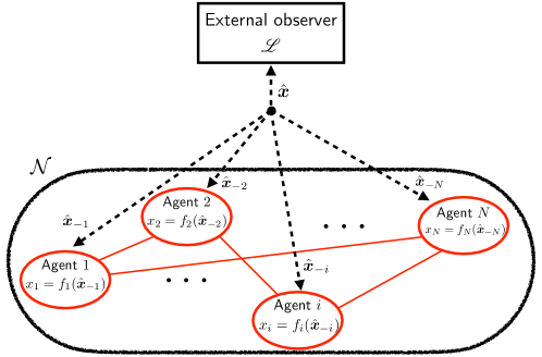
Figure 1: An external observer, endowed with some learning procedure $\mathscr{L}$, is allowed to make queries $\hat{\boldsymbol{x}}$ and observe the reactions taken by a set of $N$ agents through private action-reaction mappings, $f_{i}(\cdot)$, aiming at learning them to predict an outcome of the underlying multi-agent interaction process.

Unlike the works above, we design an active learning scheme that allows an agnostic external entity to reproduce faithful approximations of action-reaction mappings, privately held by a population of competitive agents, in order to predict a desirable outcome of the underlying multi-agent interaction process exactly, identified as a stationary profile.

Specifically, we consider the scenario illustrated in Fig. 1 and mathematically formalized in §II-A, where such an external observer, endowed with a learning procedure $\mathscr{L}$, can get samples of the action-reaction mappings $f_{i}(\cdot)$ of each agent $i$, for all $i=1,\ldots,N$; in particular, the external observer iteratively proposes to agent $i$ a configuration $\hat{\boldsymbol{x}}_{-i}$ of possible other agents’ decisions and gets back the reaction $x_{i}=f_{i}(\hat{\boldsymbol{x}}_{-i})$ of the agent to that configuration (see also the different tasks reported in Algorithm 1). The proposed scheme is of active learning nature in that the queries $\hat{\boldsymbol{x}}_{-i}$ are generated based on the current surrogate models $\hat{f}_{i}(\cdot)$ of the agents’ responses. We stress that, in our framework, the low-level interaction among agents is not particularly relevant in the sense that they are left free to interact with each other. On the contrary, we mainly focus on the external entity, which iteratively makes queries to estimate private action-reaction mappings with the ultimate goal of predicting a collective fixed point $\boldsymbol{x}^{\star}$ corresponding to a stationary profile. We summarize our contributions as follows:

1. An active learning algorithm allowing an external entity to collect sensible data and update parametric estimates of the agents’ action-reaction mappings;

2. Sufficient conditions to assess the asymptotic properties of the proposed active learning scheme so that, if convergence happens, it can only be towards a stationary action profile. This fact entails two main implications:

   1. Learning locally exact surrogates of the action-reaction mappings allows the external observer to succeed in its prediction task;

   2. Working with very general assumptions, the established conditions also serve as certificates for the existence of a stationary action profile.

3. A demonstration of the practical effectiveness of our methodology through extensive numerical simulations on typical multi-agent control and decision-making problems, including generalized Nash games and competitive linear feedback design problems.

To the best of our knowledge, this work represents a first attempt integrating traditional machine learning paradigms within a smart query process, with the overall goal of predicting a possible outcome in multi-agent decision-making and control problems in which the decision policies of the agents are private. As illustrated throughout the paper, we note that the scenario considered here covers a wide variety of multi-agent problems featuring competitive and cooperative interactions.

I-C Paper organization

In §II we formalize and properly motivate the learning problem addressed, while in §III we establish some preliminary, technical results. In §IV, instead, we introduce our active learning scheme and establish the asymptotic properties of the resulting learning process, which is then accompanied by a technical discussion in §V, also paving the way to possible extensions. Finally, in §VI we verify the practical effectiveness of the proposed active learning method through extensive numerical simulations. The proofs of the technical results of the paper are all deferred to Appendix A, while Appendix A-B reports suitable mathematical derivations adopted in the implementation of the proposed approach.

Notation

$\mathbb{N}$, $\mathbb{R}$ and $\mathbb{R}_{\geq 0}$ denote the set of natural, real, and nonnegative real numbers, respectively. $\mathbb{N}_{0}\coloneqq\mathbb{N}\cup\{0\}$, while $\bar{\mathbb{R}}\coloneqq\mathbb{R}\cup\{+\infty\}$ identifies the set of extended real numbers. Given a matrix $A\in\mathbb{R}^{n\times n}$, $A^{\top}$ denotes its transpose, while $A\succ 0$ ($\succcurlyeq 0$) denotes that $A$ is a positive (semi)definite matrix. Given a vector $v\in\mathbb{R}^{n}$ and a matrix $A\succ 0$, we denote by $\|v\|_{2}$ the standard Euclidean norm, while by $\|\cdot\|_{A}$ the $A$–induced norm $\|v\|_{A}\coloneqq\sqrt{v^{\top}Av}=\sqrt{\langle Av,v\rangle}$, where $\langle\cdot,\cdot\rangle:\mathbb{R}^{n}\times\mathbb{R}^{n}\rightarrow\mathbb{R}$ stands for the standard inner product. $\mathcal{B}_{\theta}(\bar{x})$ represents the $n$-dimensional ball centred around $\bar{x}$ with radius $\theta>0$, i.e., $\mathcal{B}_{\theta}(\bar{x})\coloneqq\left\{x\in\mathbb{R}^{n}\ \left|\ \|x-\bar{x}\|_{2}\leq\theta\right.\right\}$. $I_{n}$, $\boldsymbol{1}_{n}$, and $\boldsymbol{0}_{n}$ denote the $n\times n$ identity matrix, the vector of all $1$, and $0$, respectively (we omit the dimension $n$ whenever clear). Given a set $\mathcal{X}\subseteq\mathbb{R}^{n}$, $\iota_{\mathcal{X}}:\mathbb{R}^{n}\to\bar{\mathbb{R}}$ denote the associated indicator function, i.e., $\iota_{\mathcal{X}}(x)=0$ if $x\in\mathcal{X}$, $\iota_{\mathcal{X}}(x)=+\infty$ otherwise. The operator $\mathrm{col}(\cdot)$ stacks its arguments in column vectors or matrices of compatible dimensions. For example, given vectors $x_{1},\dots,x_{N}$ with $x_{i}\in\mathbb{R}^{n_{i}}$ and $\mathcal{N}=\{1,\dots,N\}$, we denote $\boldsymbol{x}\coloneqq(x_{1}^{\top},\dots,x_{N}^{\top})^{\top}=\mathrm{col}((x_{i})_{i\in\mathcal{N}})\in\mathbb{R}^{n}$, $n\coloneqq\sum_{i\in\mathcal{N}}n_{i}$, and $\boldsymbol{x}_{-i}\coloneqq\mathrm{col}((x_{j})_{j\in\mathcal{N}\setminus\{i\}})$. With a slight abuse of notation, we sometimes use also $\boldsymbol{x}=(x_{i},\boldsymbol{x}_{-i})$. The uniform distribution on the interval $[a,b]$ is denoted by $\mathcal{U}(a,b)$.

II Learning problem

We now formalize the learning problem addressed, which is successively motivated through two multi-agent control and decision-making problems that fit the framework we investigate.

II-A Mathematical formulation

We consider the scenario illustrated in Fig. 1. Here, an external observer (or entity) is allowed to make queries and observe the reactions taken by a set of $N$ (possibly competitive) agents, indexed by $\mathcal{N}\coloneqq\{1,\ldots,N\}$, which mutually influence each other. Specifically, we assume that each agent controls a vector of variables $x_{i}\in\mathbb{R}^{n_{i}}$ to react, by means of a private action-reaction mapping $f_{i}:\mathbb{R}^{n_{-i}}\to\mathbb{R}^{n_{i}}$, to the other agents’ actions $\boldsymbol{x}_{-i}\in\mathbb{R}^{n_{-i}}$, $n_{-i}\coloneqq\sum_{j\in\mathcal{N}\setminus\{i\}}n_{j}$. Within the multi-agent interaction process, the whole population of agents has also to meet collective constraints, i.e., $\boldsymbol{x}\coloneqq(x_{i},\boldsymbol{x}_{-i})\in\Omega\subseteq\mathbb{R}^{n}$, $n\coloneqq n_{i}+n_{-i}$, which are known to every agent and the external entity, and whose portion involving the $i$-th agent can be embedded directly within the action choice $f_{i}(\cdot)$. Specifically, for any given $\boldsymbol{x}_{-i}$, $f_{i}(\boldsymbol{x}_{-i})$ is so that $(f_{i}(\boldsymbol{x}_{-i}),\boldsymbol{x}_{-i})\in\Omega$, for all $i\in\mathcal{N}$. We assume that possible additional local constraints $x_{i}\in\mathcal{X}_{i}$, such as lower and upper bounds on $x_{i}$, are either private (i.e., unknown to the other agents and the external entity), or shared. In both cases, it always holds that the resulting values $f_{i}(\boldsymbol{x}_{-i})\in\mathcal{X}_{i}$. In the former case, this is a de facto situation that the external observer and the other agents take cognizance of. In the latter case, we assume that $x_{i}\in\mathcal{X}_{i}$ is already embedded in the collective constraint $\boldsymbol{x}\in\Omega$.

Being completely agnostic on the overall multi-agent interaction process and main quantities involved, we assume the underlying external entity endowed with some parametric learning procedure $\mathscr{L}$, which exploits non-private data (i.e., the decisions $f_{i}(\boldsymbol{x}_{-i})$) collected iteratively from the agents through a query process. Specifically, the main goal of the external entity is to learn, at least locally, faithful surrogates $\hat{f}_{i}$ (formally defined later in this section) of the unknown mappings $f_{i}(\cdot)$ in order to predict a desirable outcome of the multi-agent interaction process, here identified in accordance with the following definition:

Definition 2.1.

(Stationary action profile) A collective action profile $\boldsymbol{x}^{\star}\in\Omega$ is stationary if, for all $i\in\mathcal{N}$, $x^{\star}_{i}=f_{i}(\boldsymbol{x}^{\star}_{-i})$. $\square$

Coinciding with a fixed point of the action-reaction mappings characterizing the $N$ agents, the definition of stationary action profile is widely inspired by the game-theoretic notion of Nash equilibrium [9]. Given a stationary profile, indeed, none of the agents has incentive to deviate from the action currently taken. We will discuss in §II-B (and §V-B when introducing a generalization of the problem investigated) suitable multi-agent control and decision-making applications calling for a stationarity condition as the one in Definition 2.1.

We now state some conditions on the formalized problem that we assume will hold true throughout the paper:

Standing Assumption 2.2 (Mappings and constraints).

For all $i\in\mathcal{N}$, the single-valued mapping $f_{i}:\mathbb{R}^{n_{-i}}\to\mathbb{R}^{n_{i}}$ is continuous. In addition, the set $\Omega\subseteq\mathbb{R}^{n}$ of feasible collective actions is nonempty. $\square$

While the non-emptiness of $\Omega$ is an obvious requirement for the problem to be solvable, continuity of $f_{i}$ is a technical, yet not very restrictive, condition needed to prove our results.

As mentioned above, we endow the external observer with a learning procedure $\mathscr{L}$ to produce faithful proxies of the action-reaction mappings $f_{i}(\cdot)$ executed by the agents. Specifically, we let $\hat{f}_{i}:\mathbb{R}^{n_{-i}}\times\mathbb{R}^{p_{i}}\to\mathbb{R}^{n_{i}}$ denote the mapping of agent $i$ as estimated by the external entity, which is parametrized by a vector $\theta_{i}\in\mathbb{R}^{p_{i}}$ to be updated iteratively by integrating data retrieved from the agents through a query process as will be described in §IV.

Since our technical analysis will only require $\hat{f}_{i}(\cdot,\theta_{i})$ to approximate $f_{i}(\cdot)$ locally around a possible stationary action, for simplicity, we parameterize $\hat{f}_{i}(\cdot,\theta_{i})$ as the affine mapping

$$\hat{f}_{i}(\boldsymbol{x}_{-i},\theta_{i})=\Lambda_{i}\begin{bmatrix}\boldsymbol{x}_{-i}\\ 1\end{bmatrix},$$ (1)

for a matrix of coefficients $\Lambda_{i}\in\mathbb{R}^{n_{i}\times(n_{-i}+1)}$ (in this case, $\theta_{i}$ is the vectorization of $\Lambda_{i}$, with $p_{i}=n_{i}(n_{-i}+1)$). In §IV-B we will show that even such a simple surrogate mapping actually guarantees the external entity to succeed in its prediction task. The case involving a generic $\hat{f}_{i}(\cdot,\theta_{i})$ will be discussed in §V-C.

Finally, we remark that the conditions postulated in Standing Assumption 2.2 on the multi-agent interaction process are very general and, as a result, they do not even guarantee the existence of a stationary action profile in the sense of Definition 2.1. As a distinct feature of our approach, we will show that sufficient conditions can be established to assess the asymptotic properties of the proposed learning-based algorithm so that, if convergence happens, it can only be towards a stationary action profile, thus also providing certificates for the existence of the latter.

II-B Applications in multi-agent control and decision-making

II-B1 Learning equilibria in generalized Nash games

In view of the considered interaction structure at the multi-agent level, the learning problem just introduced shares similarities with the centralized learning of a generalized Nash equilibrium (GNE) in (generalized) Nash games. In fact, a generalized Nash equilibrium problem (GNEP) [9] typically involves a population of $N$ agents where each one of them aims at minimizing a predefined cost function $J_{i}:\mathbb{R}^{n}\to\mathbb{R}$ that depends both on its own (locally constrained) decision $x_{i}\in\mathcal{X}_{i}\subseteq\mathbb{R}^{n_{i}}$, as well as on the decisions of all the other agents $\boldsymbol{x}_{-i}$. In addition to local constraints, the selfish agents also compete for shared resources, and are thus required to satisfy coupling constraints, i.e., $(x_{i},\boldsymbol{x}_{-i})\in\Omega\subseteq\mathbb{R}^{n}$. The resulting game is hence defined by a collection of mutually coupled optimization problems:

$$\forall i\in\mathcal{N}:\left\{\begin{aligned} &\underset{x_{i}\in\mathcal{X}_{i}}{\textrm{min}}&&J_{i}(x_{i},\boldsymbol{x}_{-i})\\ &\textrm{ s.t. }&&(x_{i},\boldsymbol{x}_{-i})\in\Omega.\end{aligned}\right.$$ (2)

A key notion is represented here by the GNE, which typically identifies a desirable outcome of the noncooperative multi-agent decision-making process. In particular, by introducing $f_{i}(\boldsymbol{x}_{-i})=\textrm{argmin}_{y_{i}\in\mathcal{X}_{i}(\boldsymbol{x}_{-i})}\;J_{i}(y_{i},\boldsymbol{x}_{-i})$ as the so-called best-response (BR) mapping, single-valued under strict convexity of $x_{i}\mapsto J_{i}(x_{i},\boldsymbol{x}_{-i})$, and $\mathcal{X}_{i}(\boldsymbol{x}_{-i})\coloneqq\left\{x_{i}\in\mathcal{X}_{i}\ \left|\ (x_{i},\boldsymbol{x}_{-i})\in\Omega\right.\right\}$, a GNE $\boldsymbol{x}^{\star}$ amounts to a fixed point of the stack of the BR mappings of the agents, i.e., $x^{\star}_{i}=f_{i}(\boldsymbol{x}_{-i}^{\star})$ for all $i\in\mathcal{N}$.

The decision-making scenario just described clearly mirrors the problem considered in this paper. In this way, a GNE coincides with a stationary action profile as in Definition 2.1, and an external entity aims at reconstructing the BR mappings of the agents to predict a possible outcome of the observed GNEP, i.e., a GNE. Note that, also in this case, the assumptions made in Standing Assumption 2.2 are not sufficient to guarantee the existence of a Nash equilibrium profile.

II-B2 Multi-agent feedback controller synthesis

Inspired by traditional decentralized control synthesis problems [28, 29], we consider a competitive version in which each agent within a population of $N$ wants to stabilize some prescribed output $y_{i}\in\mathbb{R}^{n_{y_{i}}}$ of a global dynamical system, a goal that may be shared with other agents, by manipulating a subvector $u_{i}\in\mathbb{R}^{n_{u_{i}}}$ of control inputs. The overall linear time-invariant (LTI) dynamics thus reads as:

$$\left\{\begin{aligned} &z(k+1)=Az(k)+\sum_{i\in\mathcal{N}}B_{i}u_{i}(k),\\ &y_{i}(k)=C_{i}z(k),\text{ for all }i\in\mathcal{N},\end{aligned}\right.$$ (3)

where $z\in\mathbb{R}^{n_{z}}$ denotes the full state vector, $A\in\mathbb{R}^{n_{z}\times n_{z}}$ and $B=[B_{1}\ \ldots\ B_{N}]\in\mathbb{R}^{n_{z}\times n_{u}}$, $n_{u}\coloneqq\sum_{i\in\mathcal{N}}n_{u_{i}}$, the matrices of the state-update function, with $B_{i}\in\mathbb{R}^{n_{z}\times n_{u_{i}}}$, and $C_{i}\in\mathbb{R}^{n_{y_{i}}\times n_{z}}$ the $i$-th output matrix. We assume each pair $(A,B_{i})$ controllable and $(A,C_{i})$ observable, for all $i\in\mathcal{N}$. Note that while the input vector $u=\mathrm{col}((u_{i})_{i\in\mathcal{N}})\in\mathbb{R}^{n_{u}}$ is partitioned in $N$ subvectors, the output vectors $y_{i}$ are rather arbitrary linear combinations of the full state $z$, for example $y_{i}$ and $y_{j}$ might contain overlapping subvectors of $z$. In case each agent adopts a linear, full-state feedback controller $u_{i}(z(k))=\kappa_{i}z(k)$, the overall control design then reduces to synthesizing linear gains $\kappa_{i}\in\mathbb{R}^{n_{u_{i}}\times n_{z}}$. Taking the perspective of the $i$-th agent, the state evolution in (3) turns into:

$$z(k+1)=\underbrace{\left(A+\sum_{j\in\mathcal{N}\setminus\{i\}}B_{j}\kappa_{j}\right)}_{\eqqcolon A_{i}(\boldsymbol{\kappa}_{-i})=A_{i}}z(k)+B_{i}\kappa_{i}z(k).$$

In case each agent has full knowledge of the global model $(A,B)$ and is interested in minimizing a standard infinite-horizon cost as local performance index $J_{i}(\kappa_{i},\boldsymbol{\kappa}_{-i})=\sum_{k=0}^{\infty}\left(y_{i}(k)^{\top}Q_{i}y_{i}(k)+u^{\top}_{i}(k)R_{i}u_{i}(k)\right)$, $R_{i}\succ 0$ and $Q_{i}\succcurlyeq 0$, the $i$-th action-reaction mapping in this case reads as:

$$f_{i}(\boldsymbol{\kappa}_{-i})=\left\{\kappa_{i}\in\mathbb{R}^{n_{z}}\ \left|\ \begin{aligned} &\kappa^{\top}_{i}=\left(R_{i}+B_{i}^{\top}P_{i}B_{i}\right)^{-1}B_{i}^{\top}P_{i}A_{i},\\ &A_{i}^{\top}P_{i}A_{i}-A_{i}^{\top}P_{i}B_{i}\left(R_{i}+B_{i}^{\top}P_{i}B_{i}\right)^{-1}B_{i}^{\top}P_{i}A_{i}+\bar{Q}_{i}=0,\\ &P_{i}\succcurlyeq 0\end{aligned}\right.\right\},$$ (4)

where $\bar{Q}_{i}\coloneqq C_{i}^{\top}Q_{i}C_{i}$. Each agent thus aims at designing a standard linear quadratic regulator (LQR) trying to stabilize only the particular output of interest $y_{i}$ so that (3) is steered to the origin. Note that whenever a solution to each algebraic Riccati equation (ARE) in (4) exists and is unique, every action-reaction mapping $f_{i}(\cdot)$ happens to be single-valued.

However, since the evolution of each $y_{i}$ heavily depends on the linear gains $\kappa_{j}$, $j\in\mathcal{N}\setminus\{i\}$, the outputs $y_{i}$’s can be partially overlapping, and the weights $Q_{i}$ are individually chosen, a conflicting scenario among agents’ decisions may be triggered. The solution of the underlying multi-agent feedback controller synthesis thus calls for a collective action profile in the spirit of Definition 2.1. Note that, in case such a profile does exist, then it is necessarily stabilizing since (4) requires that, for fixed $\boldsymbol{\kappa}_{-i}$, $(A_{i}(\boldsymbol{\kappa}_{-i})+B_{i}\kappa_{i})$ has eigenvalues strictly inside the unit circle for all $i\in\mathcal{N}$. Establishing the existence of a collective action profile a-priori, however, is less obvious.

III Preliminary results

We now provide general convergence results, under certain assumptions, whose proofs are reported in the Appendix. Such results will be further specialized in §IV-B to establish the properties of our active learning scheme.

Then, consider a generic function $f:\mathbb{R}^{n}\times\mathbb{R}^{p}\to\mathbb{R}$, which we evaluate as $f(x,\theta)$ with $x\in\mathbb{R}^{n}$ and $\theta\in\mathbb{R}^{p}$, and some feasible set $\mathcal{X}\subseteq\mathbb{R}^{n}$ satisfying the following conditions:

Assumption 3.1.

The set $\mathcal{X}$ is convex. Moreover, for all $\theta\in\mathbb{R}^{p}$, $x\mapsto f(x,\theta)$ is a convex function. $\square$

Assumption 3.2.

The set $\mathcal{X}$ is bounded and nonempty. Moreover, it holds that:

1. For all $x\in\mathcal{X}$, $\theta\mapsto f(x,\theta)$ is convex and differentiable;

2. For all $\theta\in\mathbb{R}^{p}$, $x\mapsto f(x,\theta)$ is continuous;

3. For all $\theta\in\mathbb{R}^{p}$, the vector $\partial f(x,\theta)/\partial\theta\in\mathbb{R}^{p}$ of partial derivatives is bounded with respect to (w.r.t.) $x$. $\square$

Lemma 3.3.

Let Assumption 3.1 hold true. Then, given any $\theta\in\mathbb{R}^{p}$, the set $\mathcal{M}(\theta)\coloneqq{\textnormal{{argmin}}}_{y\in\mathcal{X}}~{}f(y,\theta)$ is convex. If also Assumption 3.2 holds true, then the value function $f^{\star}:\mathbb{R}^{p}\to\mathbb{R}$, $f^{\star}(\theta)\coloneqq\textnormal{{min}}_{y\in\mathcal{X}}~{}f(y,\theta)$, is continuous. $\square$

Before proceeding further, we recall some basic definitions from [30] useful for the remainder of this section:

Definition 3.4 (Lower semicontinuity, [30, Def. 1.5]).

A function $h:\mathbb{R}^{n}\to\bar{\mathbb{R}}$ is lower semicontinuous if, for all $\tilde{x}\in\mathbb{R}^{n}$,

$$\lim_{x\rightarrow\tilde{x}}\inf h(x)\coloneqq\lim_{\varepsilon\rightarrow 0}\left(\inf_{y\in\mathcal{B}_{\varepsilon}(\tilde{x})}h(y)\right)\geq h(\tilde{x}). \square$$

Definition 3.5 (Level-boundedness, [30, Def. 1.16]).

A function $g:\mathbb{R}^{n}\times\mathbb{R}^{p}\to\bar{\mathbb{R}}$ is level-bounded in $x$ locally uniformly in $\theta$ if, for all $\tilde{\theta}\in\mathbb{R}^{p}$ and $\alpha\in\mathbb{R}$, there exists a neighbourhood $\mathcal{I}=\mathcal{I}(\tilde{\theta})\subseteq\mathbb{R}^{p}$ and a bounded set $\mathcal{S}\subset\mathbb{R}^{n}$ such that $\left\{x\in\mathbb{R}^{n}\ \left|\ g(x,\theta)\leq\alpha\right.\right\}\subset\mathcal{S}$ for all $\theta\in\mathcal{I}$. $\square$

Lemma 3.6.

Let Assumption 3.1 and 3.2 hold true. Moreover, let $\mathcal{X}$ be a closed set. Then, the function $\bar{f}:\mathbb{R}^{n}\times\mathbb{R}^{p}\to\bar{\mathbb{R}}$, defined as $\bar{f}(x,\theta)\coloneqq f(x,\theta)+\iota_{\mathcal{X}}(x)$ is lower semicontinuous and level-bounded in $x$ locally uniformly in $\theta$. $\square$

We conclude this section with the following result establishing the convergence of the sequence of minimizers for $f$ with minimum norm, $\{x^{k}\}_{k\in\mathbb{N}}$. Specifically, given some $\theta^{k}\in\mathbb{R}^{p}$ the corresponding element $x^{k}$ is defined as follows:

$$x^{k}\coloneqq{} \underset{y\in\mathbb{R}^{n}}{\textrm{argmin}} \tfrac{1}{2}\|y\|_{2}^{2}$$ (5)

   s.t. $$y\in\mathcal{M}(\theta^{k}).$$

Lemma 3.7.

Let Assumption 3.1 and 3.2 hold true, and assume that $\mathcal{X}$ is also closed. Let $\{\theta^{k}\}_{k\in\mathbb{N}}$ be a sequence so that $\lim_{k\rightarrow\infty}\theta^{k}=\tilde{\theta}$, and let $\mathcal{M}(\tilde{\theta})=\{\tilde{x}\}$. Then, the sequence $\{x^{k}\}_{k\in\mathbb{N}}$ generated by (5) is feasible and satisfies $\lim_{k\rightarrow\infty}x^{k}=\tilde{x}.$ $\square$

The technical results just introduced will be instrumental to establish the asymptotic properties of the active learning scheme presented in the next section. Specifically, we will see in §IV-B how the proposed method meets Assumption 3.1 and 3.2 to exploit the convergence of the sequence of minimum-norm minimizers of a suitable collection of parametric programs.

IV Active learning procedure and main results

Armed with the notions and preliminary results introduced in the previous sections, we now propose and discuss the asymptotic properties of a scheme in which, by actively learning local surrogates of the private action-reaction mappings through an iterative sample collection procedure, the external entity attempts to converge to a stationary action profile.

IV-A Algorithm description

Initialization: $\boldsymbol{x}^{0}\in\Omega$, $\theta_{i}^{0}\in\mathbb{R}^{p_{i}}\text{ for all }i\in\mathcal{N}$

Iteration $(k\in\mathbb{N}_{0})$:

• $\theta_{i}^{k+1}\in\underset{\xi_{i}\in\mathbb{R}^{p_{i}}}{\textrm{argmin}}\;\frac{1}{k}\sum_{t=1}^{k}\ell_{i}(x_{i}^{t},\hat{f}_{i}(\hat{\boldsymbol{x}}^{t}_{-i},\xi_{i})),\forall i\in\mathcal{N}$

• $\hat{\boldsymbol{x}}^{k+1}=\underset{\boldsymbol{y}\in\mathbb{R}^{n}}{\textrm{argmin}}~{}\tfrac{1}{2}\|\boldsymbol{y}\|_{2}^{2}~{}\textrm{ s.t. }~{}\boldsymbol{y}\in\mathcal{M}(\theta^{k+1})$

• $\text{For all }i\in\mathcal{N}:x^{k+1}_{i}=f_{i}(\hat{\boldsymbol{x}}^{k+1}_{-i})$

Algorithm 1 Active learning-based method

The main steps of our active learning scheme are summarized in Algorithm 1, where the black-filled bullets refer to the tasks the external observer is required to perform, while the empty bullet to the one performed by the agents in $\mathcal{N}$. Note that in the context of Algorithm 1, the low-level interaction among agents takes a back seat in the sense that they are required to provide an answer whenever queried.

Thus, at the generic $k$-th iteration of Algorithm 1, the external entity updates the affine surrogate mappings $\hat{f}_{i}(\cdot,\theta_{i}^{k})$ including the most recent samples according to the following rule:

$$\theta_{i}^{k+1}\in\underset{\xi_{i}\in\mathbb{R}^{p_{i}}}{\textrm{argmin}}\;\frac{1}{k}\sum_{t=1}^{k}\ell_{i}(x_{i}^{t},\hat{f}_{i}(\hat{\boldsymbol{x}}^{t}_{-i},\xi_{i}))\eqqcolon\Theta_{i}(\left\{(x_{i}^{t},\hat{\boldsymbol{x}}^{t}_{-i})\right\}_{t=1}^{k})=\Theta_{i}^{k},\text{ for all }i\in\mathcal{N},$$ (6)

where $\ell_{i}:\mathbb{R}^{n}\times\mathbb{R}^{p_{i}}\to\mathbb{R}$ is some loss function, typically dictated by the function approximation type adopted and the problem at hand. Referring to Algorithm 1, we preliminarily define, for all $i\in\mathcal{N}$, $\textrm{argmin}_{\xi_{i}\in\mathbb{R}^{p_{i}}}\;(1/k)\sum_{t=1}^{k}\ell_{i}(x_{i}^{t},\hat{f}_{i}(\hat{\boldsymbol{x}}^{t}_{-i},\xi_{i}))\eqqcolon\Theta_{i}(\left\{(x_{i}^{t},\hat{\boldsymbol{x}}^{t}_{-i})\right\}_{t=1}^{k})=\Theta_{i}^{k}$. By referring to Fig. 1, the vector $\hat{\boldsymbol{x}}^{t}$ hence denotes the query point employed by the external entity at the $t$-th iteration to gather all the best responses $f_{i}(\hat{\boldsymbol{x}}^{t}_{-i})$.

Successively, by relying on the updated proxies for the agents’ action-reaction mappings $\hat{f}_{i}$, the external entity chooses the next query point $\hat{\boldsymbol{x}}^{k+1}$ as the minimum norm strategy profile in the set $\mathcal{M}:\mathbb{R}^{p}\to 2^{\Omega}$, $p\coloneqq\sum_{i\in\mathcal{N}}p_{i}$, formally defined as:

$$\mathcal{M}(\theta^{k+1})\coloneqq\underset{\boldsymbol{y}\in\Omega}{\textrm{argmin}}\;\sum_{i\in\mathcal{N}}\left\|y_{i}-\hat{f}_{i}(\boldsymbol{y}_{-i},\theta^{k+1}_{i})\right\|^{2}_{2},$$ (7)

which contains all collective profiles that are the closest (according to the squared Euclidean norm, although different metrics could be used) to a fixed point of each $\hat{f}_{i}(\cdot,\theta_{i}^{k+1})$. This step is motivated by the notion of stationary action profile in Definition 2.1, which coincides with a fixed point of the stack of the agents’ mappings, i.e., $x_{i}^{\star}=f_{i}(\boldsymbol{x}_{-i}^{\star})$ for all $i\in\mathcal{N}$. Indeed, if $\hat{f}_{i}$ were exactly equal to $f_{i}$ and the minimum in (7) were zero, any $\boldsymbol{x}^{\star}\in\mathcal{M}(\theta^{k+1})$ would be a stationary action profile. Note that, by referring to (7), $\theta^{k+1}$ identifies the whole collection of parameters $\{\theta_{i}^{k+1}\}_{i\in\mathcal{N}}$ characterizing the surrogate mappings, which at every iteration represent the argument of the corresponding parameter-to-query mapping $\mathcal{M}(\cdot)$.

Under the special choice in (1), program (7) turns out to be a constrained LS problem, which is convex whenever $\Omega$ is convex. To simplify notation, assume $n_{i}=1$ for all $i\in\mathcal{N}$ so that $\Lambda_{i}=[\nu_{i}^{\top}\;c_{i}]$ in (1) (the extension to the case $n_{i}\geq 2$ follows readily). Then, the minimization problem (7) becomes:

$$\underset{\boldsymbol{y}\in\Omega}{\textrm{min}}\;\sum_{i\in\mathcal{N}}\left\|y_{i}-(\nu^{k+1}_{i})^{\top}\boldsymbol{y}_{-i}-c^{k+1}_{i}\right\|^{2}_{2}.$$ (8)

Moreover, in the absence of constraints ($\Omega=\mathbb{R}^{n}$), we can further characterize the stationary action profile we wish to compute. In fact, problem (7) can be solved by imposing $y_{i}-\hat{f}_{i}(\boldsymbol{y}_{-i},\theta_{i})=y_{i}-\nu^{\top}_{i}\boldsymbol{y}_{-i}-c_{i}=0$ for all $i\in\mathcal{N}$, therefore getting the following system of $N$ equations with $N$ unknowns:

$$\begin{bmatrix}1&&-\nu_{1}^{\top}\\ \vdots&\ddots&\vdots\\ -\nu_{N}^{\top}&&1\end{bmatrix}\boldsymbol{y}=\begin{bmatrix}c_{1}\\ \vdots\\ c_{N}\end{bmatrix},$$ (9)

where the superscript ^k+1 has been omitted for simplicity. In particular, if (9) is solvable, every solution lies on a subspace $\mathcal{M}(\theta^{k+1})$ of dimension smaller than $N$ (a single point when it is unique), and the vector $\hat{\boldsymbol{x}}^{k+1}$ corresponds to the minimum-norm solution of (9). When $\Omega\subset\mathbb{R}^{n}$, one might still be tempted to solve (9) to get the next query point $\hat{\boldsymbol{x}}^{k+1}$. However, further queries may return infeasible reactions by some of the agents, as shown in the pictorial representation in Fig. 2.

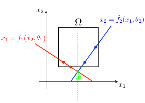
Figure 2: Consider $N=2$ agents controlling a scalar decision variable, and both $\hat{f}_{i}$ are affine surrogates constructed using feasible samples (red and blue dots) in $\Omega$ (black box). Solving (9) would return the green point as a unique global minimizer (green dot) outside $\Omega$. While agent number $2$ can still provide a feasible reaction to this infeasible query point, as it has to make a decision along the dashed blue line, agent $1$ can not (decision to be made along the dashed red line).

The postulated assumptions are not sufficient to guarantee the existence of a vector $\boldsymbol{x}^{\star}$ such that $\left\|x^{\star}_{i}-f_{i}(\boldsymbol{x}^{\star}_{-i})\right\|_{2}=0$ for all $i\in\mathcal{N}$. We will establish in our main result (i.e., Theorem 4.5), sufficient conditions for the existence of such a vector $\boldsymbol{x}^{\star}$.

Once obtained the minimum norm vector $\hat{\boldsymbol{x}}^{k+1}$ in (7), this serves as a query profile to collect the next agents’ reaction data, $x^{k+1}_{i}=f_{i}(\hat{\boldsymbol{x}}^{k+1}_{-i})$. Within the final step of the procedure, indeed, $\hat{\boldsymbol{x}}^{k+1}$ is broadcasted to the agents, which on their side react to $\hat{\boldsymbol{x}}^{k+1}_{-i}$ by computing $f_{i}(\cdot)$, and finally return the results to the external entity. Therefore, each $x^{k+1}_{i}$ enriches the training dataset used in (6) to improve the affine model $\hat{f}_{i}(\cdot,\theta_{i}^{k+1})$.

IV-B Asymptotic properties

Before characterizing the asymptotic properties of the active learning procedure in Algorithm 1, we first postulate some assumptions on the learning procedure $\mathscr{L}$ the external observer is endowed with and then establish some results, whose proofs are reported in the Appendix, that will be instrumental for the main statement of the paper.

Standing Assumption 4.1 (Training loss).

For all $i\in\mathcal{N}$, the loss function $\ell_{i}$ is continuous in both arguments and, for all $(x_{i},\boldsymbol{x}_{-i},\theta_{i})\in\Omega\times\mathbb{R}^{p_{i}}$, $0\leq\ell_{i}(x_{i},\hat{f}_{i}(\boldsymbol{x}_{-i},\theta_{i}))<\infty$, with $\ell_{i}(x_{i},\hat{f}_{i}(\boldsymbol{x}_{-i},\theta_{i}))=0$ if and only if $x_{i}=\hat{f}_{i}(\boldsymbol{x}_{-i},\theta_{i})$. $\square$

The conditions reported in Standing Assumption 4.1 allow to characterize the choice of the loss functions adopted in (6).

A key property possessed by the affine surrogates $\hat{f}_{i}(\cdot,\theta_{i})$, which will be key to prove our main result, is the possibility to match pointwise (and, therefore, not necessarily globally nor even locally) the action-reaction mapping $f_{i}$ of each agent. Specifically, for all $i\in\mathcal{N}$ and for all $(x_{i},\boldsymbol{x}_{-i})\in\Omega$, there exists a set $\mathcal{A}_{i}=\mathcal{A}_{i}(x_{i},\boldsymbol{x}_{-i})\subseteq\mathbb{R}^{p_{i}}$ such that $\ell_{i}(x_{i},\hat{f}_{i}(\boldsymbol{x}_{-i},\tilde{\theta}_{i}))=0$, for all $\tilde{\theta}_{i}\in\mathcal{A}_{i}$. While this condition is intrinsic for affine surrogates, it shall therefore be assumed to hold true in case of generic proxies $\hat{f}_{i}(\cdot,\theta_{i})$ within the discussion in §V-C. Moreover, in view of the specific structure (1) we consider, the affine proxies are also continuous with respect to their second argument, i.e., $\hat{f}_{i}(\boldsymbol{x}_{-i},\cdot)$ is continuous for all $\boldsymbol{x}_{-i}\in\mathbb{R}^{n_{-i}}$.

The crucial result stated next requires the external entity to solve (6) at the global minimum at every iteration. In case there exist multiple (global) minimizers we then tacitly assume further the external observer being endowed with a tailored tie-break rule, i.e., some single-valued mapping $\mathcal{T}:2^{\mathbb{R}^{p_{i}}}\to\mathbb{R}^{p_{i}}$ used consistently across iterations, such as picking up the solution $\theta^{k}_{i}$ with minimum norm at every $k\in\mathbb{N}$, to single-out one of those minimizers, for all $i\in\mathcal{N}$. With this tie-break rule $\mathcal{T}$ in place, which takes a set of vectors in $\mathbb{R}^{p_{i}}$ as argument and returns one element from it according to some criterion, the first step in Algorithm 1 performed by the external observer turns into an equality rather than an inclusion.

Lemma 4.2.

For all $i\in\mathcal{N}$, let $\{(x_{i}^{t},\hat{\boldsymbol{x}}^{t}_{-i})\}_{t=1}^{k}$ be a collection of samples to be employed in the update rule for the parameter $\theta_{i}$ in (6), where each $(x_{i}^{t},\hat{\boldsymbol{x}}^{t}_{-i})\in\Omega$. Assume that, for every $k\in\mathbb{N}$, (6) is solved at the global minimum and a tie-break rule $\mathcal{T}$ is applied to single-out a minimizer. If $\lim_{k\to\infty}x_{i}^{k}=\bar{x}_{i}$, $\lim_{k\to\infty}\hat{\boldsymbol{x}}^{k}_{-i}=\bar{\boldsymbol{x}}_{-i}$ so that $(\bar{x}_{i},\bar{\boldsymbol{x}}_{-i})\in\Omega$, and $\lim_{k\to\infty}\theta_{i}^{k}=\bar{\theta}_{i}$, then $\bar{\theta}_{i}\in\mathcal{A}_{i}(\bar{x}_{i},\bar{\boldsymbol{x}}_{-i})$, for all $i\in\mathcal{N}$. $\square$

Lemma 4.2 shows a sort of “consistency property” of the affine surrogates $\hat{f}_{i}$, meaning that if all the ingredients involved in Algorithm 1 happen to converge, then the pointwise approximation of $f_{i}$ shall be exact at ${\boldsymbol{x}}_{-i}$, i.e., $\hat{f}_{i}({\boldsymbol{x}}_{-i},\tilde{\theta}_{i})=f_{i}({\boldsymbol{x}}_{-i})$.

Standing Assumption 4.3 (Feasible set $\Omega$).

The set $\Omega$ is a nonempty polytope. $\square$

We now characterize the properties of the sequence of query points $\{\hat{\boldsymbol{x}}^{k}\}_{k\in\mathbb{N}}$ produced by the central entity in the second step of Algorithm 1 by computing the optimal solution to:

$$\hat{\boldsymbol{x}}^{k}\coloneqq{} \underset{\boldsymbol{y}\in\mathbb{R}^{n}}{\textrm{argmin}} \tfrac{1}{2}\|\boldsymbol{y}\|_{2}^{2}$$ (10)

   s.t. $$\boldsymbol{y}\in\mathcal{M}(\theta^{k}),$$

for all $k\in\mathbb{N}$, thus mirroring the strategy to generate $x^{k}$ in (5).

Proposition 4.4.

Let $\{\theta^{k}\}_{k\in\mathbb{N}}$ be a sequence so that $\lim_{k\to\infty}\theta_{i}^{k}=\tilde{\theta}_{i}$ for all $i\in\mathcal{N}$, and let $\mathcal{M}(\tilde{\theta})=\{\tilde{\boldsymbol{x}}\}$. Then the sequence $\{\hat{\boldsymbol{x}}^{k}\}_{k\in\mathbb{N}}$ generated by (10) is feasible and satisfies $\lim_{k\rightarrow\infty}\hat{\boldsymbol{x}}^{k}=\tilde{\boldsymbol{x}}.$ $\square$

We are now ready to state the asymptotic properties of the active learning methodology described in Algorithm 1:

Theorem 4.5.

Let $\{\theta^{k}\}_{k\in\mathbb{N}}$ be a sequence so that $\lim_{k\to\infty}\theta_{i}^{k}=\tilde{\theta}_{i}$ for all $i\in\mathcal{N}$, and let $\mathcal{M}(\tilde{\theta})=\{\tilde{\boldsymbol{x}}\}$. For every $k\in\mathbb{N}$, let (6) be solved at the global minimum and a tie-break rule $\mathcal{T}$ applied to single-out a minimizer. Then, $\lim_{k\to\infty}\|\hat{\boldsymbol{x}}^{k}-\boldsymbol{x}^{k}\|_{2}=0$, and the sequence $\{\boldsymbol{x}^{k}\}_{k\in\mathbb{N}}$ and $\{\hat{\boldsymbol{x}}^{k}\}_{k\in\mathbb{N}}$ generated by Algorithm 1 converge to the same stationary action profile.  $\square$

As a direct consequence implied by Theorem 4.5, we obtain that the external entity is actually able to succeed in its prediction task. Specifically, in case the convergence of the parametric estimates happens, it can only be towards the true (at least pointwise) values. This fact, together with $\lim_{k\to\infty}\|\hat{\boldsymbol{x}}^{k}-\boldsymbol{x}^{k}\|_{2}=0$, yields $\sum_{i\in\mathcal{N}}\|\hat{\boldsymbol{x}}_{i}-\hat{f}_{i}(\hat{\boldsymbol{x}}_{-i},\tilde{\theta}_{i})\|^{2}_{2}=\sum_{i\in\mathcal{N}}\|\hat{\boldsymbol{x}}_{i}-f_{i}(\hat{\boldsymbol{x}}_{-i})\|^{2}_{2}=0$, and hence $\|\hat{\boldsymbol{x}}_{i}-\hat{f}_{i}(\hat{\boldsymbol{x}}_{-i},\tilde{\theta}_{i})\|_{2}$ for all $i\in\mathcal{N}$, i.e., the external entity has in its hands both a stationary action profile $\hat{\boldsymbol{x}}$, and pointwise-exact surrogates of the action-reaction mappings $\hat{f}_{i}(\hat{\boldsymbol{x}}_{-i},\tilde{\theta}_{i})=f_{i}(\hat{\boldsymbol{x}}_{-i})$. The following corollary assessing the existence of at least a stationary action profile is an immediate consequence of Theorem 4.5.

Corollary 4.6.

Under the conditions stated in Theorem 4.5, the multi-agent interaction process at hand admits a stationary action profile $\boldsymbol{x}^{\star}$ in the sense of Definition 2.1. $\square$

V Technical discussion and possible extensions

In this section we elaborate around the conditions granting the asymptotic properties stated in Theorem 4.5. In addition, we discuss possible extensions to a more general framework involving the composition of action-reaction policies, or to the adoption of generic surrogate mappings for their estimate.

V-A Discussion on Theorem 4.5

Assuming that $\lim_{k\to\infty}\theta_{i}^{k}=\tilde{\theta}_{i}$ for all $i\in\mathcal{N}$, along with the existence of a single minimizer contained in $\mathcal{M}(\tilde{\theta})$ (7), appear rather strong requirements to achieve the convergence of the proposed active learning scheme that, to the best of our knowledge, can not be guaranteed beforehand, not even by imposing further structure on the learning procedure $\mathscr{L}$ or the multi-agent problem at hand. Both can indeed be verified only a-posteriori, or in practice after a large enough number of iterations of Algorithm 1. Note that, in the specific scenario of affine surrogate mappings $\hat{f}_{i}$ in (1), checking whether $\mathcal{M}(\tilde{\theta})$ is a singleton simply translates into verifying the positive definiteness of the Hessian matrix characterizing (8).

We note that, however, the technical conditions assumed in Standing Assumption 2.2 are so general that they do not even seem to be sufficient to establish the existence of a stationary action profile for the underlying problem. This should be put together with the fact that the external observer: i) has very little knowledge of such a process, ii) can be endowed with any learning procedure $\mathscr{L}$ satisfying Standing Assumption 4.1, and iii) could succeed in its prediction task even with a simple, i.e., affine, parametrization for the surrogate mappings $\hat{f}_{i}$.

In the considered framework, the a-posteriori verification of the convergence of the parametric estimates yielding a single minimizer in $\mathcal{M}(\cdot)$ brings the considerable consequence of representing a certificate for both the existence of a stationary action profile, which is not a foregone conclusion in the considered scenario, along with the possibility for the external entity to predict an outcome of the multi-agent interaction process observed. We point to §VI for many numerical results in which the a-posteriori verification step indeed succeeds, thus demonstrating the practical effectiveness of our methodology.

V-B Learning composition of action-reaction mappings

Consider the case in which the decision variable $x_{i}$ does not follow directly as a result of some reaction process through $f_{i}(\cdot)$, but it coincides with a function of some other inner variable, say $w_{i}\in\mathcal{W}_{i}\subseteq\mathbb{R}^{m_{i}}$ (in this new framework, $f_{i}$ should be suitably redefined taking $\mathbb{R}^{m_{i}}$ as codomain). By introducing $g_{i}:\mathbb{R}^{m_{i}}\to\mathbb{R}^{n_{i}}$ as an additional, private mapping we have that $x_{i}$ is obtained through the composition $(g_{i}~{}\raisebox{1.0pt}{ \leavevmode\hbox to3.1pt{\vbox to3.1pt{\text{[drawing]}}}}~{}f_{i})(\boldsymbol{x}_{-i})$, i.e.,

$$x_{i}=g_{i}(w_{i})=g_{i}(f_{i}(\boldsymbol{x}_{-i})).$$

This different perspective can be justified, for instance, by privacy reasons or simply agents’ decisions require a first pass through some additional mapping, thus making the reaction process to $\boldsymbol{x}_{-i}$ indirect. As a motivating example, consider a population of agents obeying to the following dynamics:

$$\forall i\in\mathcal{N}:\left\{\begin{aligned} &z_{i}(k+1)=d_{i}(z_{i}(k),u_{i}(k))+s_{i}(\boldsymbol{u}_{-i}(k),\boldsymbol{v}_{-i}(k)),\\ &v_{i}(k)=t_{i}(z_{i}(k),u_{i}(k)),\end{aligned}\right.$$ (11)

where $z_{i}\in\mathbb{R}^{n_{z_{i}}}$, $u_{i}\in\mathbb{R}^{n_{u_{i}}}$, and $v_{i}\in\mathbb{R}^{n_{v_{i}}}$ denote the state vector, the control input, and the controlled output of each agent, respectively, whose evolution (except for $u_{i}$, which has to be designed) is determined by mappings $d_{i}:\mathbb{R}^{n_{z_{i}}}\times\mathbb{R}^{n_{u_{i}}}\to\mathbb{R}^{n_{z_{i}}}$ and $t_{i}:\mathbb{R}^{n_{z_{i}}}\times\mathbb{R}^{n_{u_{i}}}\to\mathbb{R}^{n_{v_{i}}}$. The behavior of the state variables, however, is also affected by some function $s_{i}:\mathbb{R}^{n_{u_{-i}}}\times\mathbb{R}^{n_{v_{-i}}}$ of the other agents’ control inputs and outputs. Planning an optimal control strategy over some horizon of length $T\geq 1$ traditionally requires each agent to find a solution to the following optimal control problem:

$$\forall i\in\mathcal{N}:\left\{\begin{aligned} &\underset{w_{i}}{\textrm{min}}&&\Psi_{i}(z_{i}(T))+\sum_{k=0}^{T-1}\,\Phi_{i}(x_{i}(k),\boldsymbol{x}_{-i}(k),k)\\ &\textrm{ s.t. }&&\eqref{eq:dynamics},~{}\forall k=1,\ldots,T-1,\\ &&&z_{i}(0)=z_{i,0},\\ &&&x_{i}(k)\in\mathcal{\mathcal{missing}}X_{i},~{}\forall k=0,\ldots,T-1,\end{aligned}\right.$$ (12)

where $z_{i,0}\in\mathbb{R}^{n_{z_{i}}}$ is the measured initial state, $w_{i}(k)=\mathrm{col}(u_{i}(k),z_{i}(k+1))$, $w_{i}\coloneqq\mathrm{col}((w_{i}(k))_{k=0}^{T-1})\in\mathbb{R}^{n_{w_{i}}}$, $n_{w_{i}}\coloneqq T(n_{u_{i}}+n_{z_{i}})$, $x_{i}(k)\coloneqq\mathrm{col}(u_{i}(k),v_{i}(k))\in\mathbb{R}^{n_{u_{i}}+n_{v_{i}}}$, with $x_{i}\coloneqq g(w_{i})=\mathrm{col}((x_{i}(k))_{k=0}^{T-1})\in\mathbb{R}^{n_{i}}$, $n_{i}\coloneqq T(n_{u_{i}}+n_{v_{i}})$, $g:\mathbb{R}^{n_{w_{i}}}\to\mathbb{R}^{n_{i}}$, $\mathcal{\mathcal{missing}}X_{i}\subseteq\mathbb{R}^{n_{u_{i}}}\times\mathbb{R}^{n_{v_{i}}}$ denotes the input-output constraint set, $\Phi_{i}:\mathbb{R}^{n_{u_{i}}+n_{v_{i}}}\times\mathbb{R}^{n_{x_{-i}}}\times\mathbb{N}\to\mathbb{R}$ is the $i$-th stage cost that depends on $k$ to include a possible reference output signal to track, and $\Psi_{i}:\mathbb{R}^{n_{z_{i}}}\to\mathbb{R}$ is a terminal cost.

The exogenous term $s_{i}$ in (11) thus makes (12) a collection of optimization problems with coupling terms dependent on $\boldsymbol{x}_{-i}$ both in the cost and constraints, whose overall solution, if any, naturally calls for a collective action profile in the spirit of Definition 2.1, which in this generalized setting reads as:

$$\boldsymbol{x}^{\star}\in\Omega\text{ s.t., for all }i\in\mathcal{N},~{}x^{\star}_{i}=g_{i}(f_{i}(\boldsymbol{x}^{\star}_{-i})).$$

The agnostic external entity will therefore collect data by querying the agents with tailored opponents’ input/output profiles, and then update proxies for each composition $(g_{i}~{}\raisebox{1.0pt}{ \leavevmode\hbox to3.1pt{\vbox to3.1pt{\text{[drawing]}}}}~{}f_{i})$ to predict the optimal control actions adopted by the set of agents over the $T$-steps long horizon.

From a merely technical perspective, to let our machinery work also in this more general setting, the conditions on $f_{i}(\cdot)$ in Standing Assumption 2.2 shall be replaced with the following:

1. Each mapping $(g_{i}~{}\raisebox{1.0pt}{ \leavevmode\hbox to3.1pt{\vbox to3.1pt{\text{[drawing]}}}}~{}f_{i})(\cdot)$ is continuous and single-valued;

2. For all $\boldsymbol{x}_{-i}\in\mathbb{R}^{n_{-i}}$, $f_{i}(\boldsymbol{x}_{-i})$ produces some $w_{i}\in\mathcal{W}_{i}$ so that $(g_{i}(w_{i}),\boldsymbol{x}_{-i})\in\Omega$.

Then, nothing prevents the external entity from adopting the same affine surrogate mappings (1) to estimate each composition $(g_{i}~{}\raisebox{1.0pt}{ \leavevmode\hbox to3.1pt{\vbox to3.1pt{\text{[drawing]}}}}~{}f_{i})(\cdot)$, whereas the final step of the active learning scheme in Algorithm 1 will require to simply collect $x^{k+1}_{i}=g_{i}(f_{i}(\hat{\boldsymbol{x}}_{-i}^{k+1}))$ for all $i\in\mathcal{N}$. The technical analysis on the asymptotic properties of the variant of Algorithm 1 just discussed then mimics the one carried out in §IV-B.

V-C Generic surrogate mappings $\hat{f}_{i}$

In case one is interested in endowing the central entity with more flexible surrogate mappings $\hat{f}_{i}$ different from the affine ones in (1), some further conditions have to be imposed.

Specifically, by mirroring the discussion in §IV-B tailored for affine proxies, one shall necessarily integrate Standing Assumption 4.1 with a requirement on the continuity of the mapping $\theta_{i}\mapsto\hat{f}_{i}(\boldsymbol{x}_{-i},\theta_{i})$ for all $\boldsymbol{x}_{-i}\in\mathbb{R}^{n_{-i}}$. Nevertheless, the proxies $\hat{f}_{i}$ shall also be able to match at least pointwise the action-reaction mapping $f_{i}$ of each agent, thus requiring that for all $(x_{i},\boldsymbol{x}_{-i})\in\Omega$, there exists a set $\mathcal{A}_{i}=\mathcal{A}_{i}(x_{i},\boldsymbol{x}_{-i})\subseteq\mathbb{R}^{p_{i}}$ such that $\ell_{i}(x_{i},\hat{f}_{i}(\boldsymbol{x}_{-i},\tilde{\theta}_{i}))=0$, for all $\tilde{\theta}_{i}\in\mathcal{A}_{i}$. These two conditions together are key to prove the consistency property in Lemma 4.2 also with generic surrogate mappings. In addition, to rely on Proposition 4.4 one should also ensure that the chosen proxies $\hat{f}_{i}$ allow meeting Assumption 3.1 and Assumption 3.2 characterizing the second task performed by the external entity in Algorithm 1, so that the arguments made in the proof of Theorem 1 could be applied also to this more generic case. A main drawback of using nonlinear surrogates is that the cost function in problem (7) may easily become nonconvex.

VI Numerical results

We now test the practical effectiveness of the active learning scheme in Algorithm 1 on several numerical instances of the multi-agent control and decision-making problems in §II. All simulations are run in MATLAB on a laptop with an Apple M2 chip featuring an 8-core CPU and 16 Gb RAM.

To keep problem (6) convex and quadratic, we use the affine setting (1) along with the mean squared error (MSE) loss:

$$\ell_{i}(x_{i}^{t},\hat{f}_{i}(\hat{\boldsymbol{x}}^{t}_{-i},\xi_{i}))=\|x_{i}^{t}-\hat{f}_{i}(\hat{\boldsymbol{x}}^{t}_{-i},\xi_{i})\|_{2}^{2}.$$

Hence, due to the incremental number $k$ of training data, we can use simple recursive methods to update the estimate $\theta_{i}^{k+1}$ in (6), as described for instance in [31, 32], such as recursive LS [33]. In our numerical simulations, to control the learning-rate of the algorithm we adopt the following linear Kalman filter iterations [34] tailored for $n_{i}=1$ (see Appendix A-B for the derivation):

$$\phi_{i}^{k}=\begin{bmatrix}\hat{\boldsymbol{x}}^{k}_{-i}\\ 1\end{bmatrix},\ a_{i}^{k}=P_{i}^{k}\phi_{i}^{k}$$ (13a)

$$P^{k+\nicefrac{{1}}{{2}}}_{i}=P_{i}^{k}-\frac{a_{i}^{k}(a_{i}^{k})^{\top}}{1+(\phi_{i}^{k})^{\top}a_{i}^{k}}$$ (13b)

$$\theta_{i}^{k+1}=\theta_{i}^{k}+P_{i}^{k+\nicefrac{{1}}{{2}}}\phi_{i}^{k}(x_{i}^{k}-(\phi_{i}^{k})^{\top}\theta_{i}^{k})$$ (13c)

$$P_{i}^{k+1}=P_{i}^{k+\nicefrac{{1}}{{2}}}+\beta I$$ (13d)

In case $n_{i}>1$, a bank of KF’s as in (13) is run in parallel for each of the $n_{i}$ components of $\hat{f}_{i}$. Specifically, in (13) $\beta\geq 0$ defines the learning-rate of the Kalman filter, and the initial value of the $N$-by-$N$ covariance matrix $P_{i}^{0}=\alpha I$ the amount of $\ell_{2}$-regularization on $\theta_{i}$ (cf. [35, Eq. (12)]). In particular, the larger the $\beta$, the faster is the convergence of the linear estimator (we obtain standard recursive LS updates for $\beta=0$ [31, 32]), while the smaller the $\alpha$, the larger is the $\ell_{2}$-regularization. The tuning of $\beta$ will be discussed later in each subsection.

As commonly done in most active learning algorithms [36, 37, 38], the execution of Algorithm 1 is preceded by a (passive) random data collection phase to make an initial estimate of the affine surrogates $\hat{f}_{i}$. During this initialization procedure, the external entity draws iteratively a random feasible point $\boldsymbol{x}^{k}\in\Omega$ as follows. First, it forms a random vector $\boldsymbol{x}_{r}^{k}\in\mathbb{R}^{n}$ by extracting its components $x_{r_{i}}^{k}$ from the uniform distribution $\mathcal{U}(m^{-}_{i},m^{+}_{i})$ where $m^{-}\leq\boldsymbol{x}\leq m^{+}$ are a known estimate of the range of $\boldsymbol{x}$. Then, the following constrained LS problem

$$\boldsymbol{x}^{k}=\underset{\boldsymbol{y}\in\Omega}{\textrm{argmin}}\;\|\boldsymbol{y}-\boldsymbol{x}_{r}^{k}\|_{2}^{2},$$

is solved to define $\boldsymbol{x}^{k}$ and pass it in parallel to each agent, which in turn responds through the private action-reaction mapping $f_{i}$. The resulting actions are collected by the external entity to update its estimates $\theta_{i}^{k}$. Lasting for a percentage $K_{\textrm{in}}$ of the total number of iterations $K$ of Algorithm 1, as expected, we noticed that this random initialization procedure affects the performance of our active learning scheme, and therefore we discuss it in details within each numerical example.

VI-A Generalized Nash games

For this multi-agent decision-making problem we consider examples from [39, 40] to cover several cases of interest.

Specifically, we start by considering the noncooperative Nash game described in [39, Ex. 1], where $N=10$ agents have cost functions $J_{i}(x_{i},\boldsymbol{x}_{-i})=N(1+(i-1)/2)x_{i}-x_{i}(60N-\boldsymbol{1}^{\top}_{N}\boldsymbol{x})$, while $\Omega=[7,100]^{N}$.

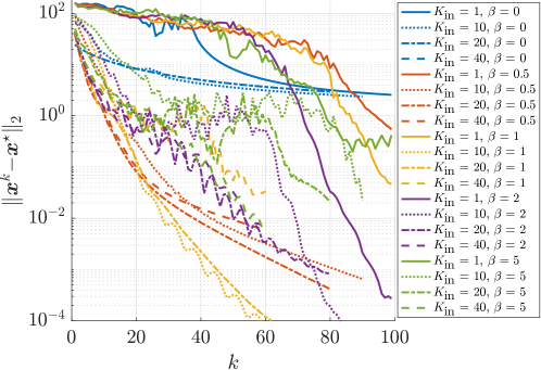
Figure 3: Hyperparameters analysis on the Nash equilibrium problem formalized in [39, Ex. 1].

We first perform a numerical analysis to set the two main hyperparameters affecting the execution of Algorithm 1, namely the learning coefficient $\beta$ and the number $K_{\textrm{in}}$ of iterations during the data collection phase. The selected values will be adopted also for the remaining numerical instances considered in this subsection. Fig. 3 illustrates the impact those hyperparameters have on the convergence of Algorithm 1 to an equilibrium of the underlying game (computed through a standard extragradient type method [41]), averaged over $20$ random initialization procedures for each coefficients combination. In particular, we have considered $\beta\in\{0,0.5,1,2,5\}$ and $K_{\textrm{in}}\in\{0.01,0.1,0.2,0.4\}\cdot K$, with $K=100$. Different rules for selecting $K_{\textrm{in}}$ can be adopted, e.g., choosing $K_{\textrm{in}}$ as a function of the dimension $n_{-i}\!-\!1$ of $\theta_{i}$.

We remark here that Theorem 4.5 ensures the convergence to some stationary action profile if the estimation parameters converge that the minimizer in (8) is unique, for which a sufficient condition is that the associated Hessian matrix $H$ is positive definite. These are conditions that depend on multiple factors and, although easily verifiable a posteriori, are unpredictable a priori. That is why one should not expect convergence in all numerical instances considered to draw Fig. 3: this fact will be explored more in detail in §VI-B through statistical analysis. What we can infer from Fig. 3 instead is that while, on the one hand, it seems that some long enough random initialization procedure is indeed required (solid lines corresponding to $K=1$ are indeed associated with the slowest behaviors), on the other hand, an exceedingly large learning rate (green and violet lines) does not appear to bring significant benefit in terms of rate of convergence. Therefore, for this subsection we decide to use $\beta=1$ and $K_{\textrm{in}}=\lceil K/10\rceil$.

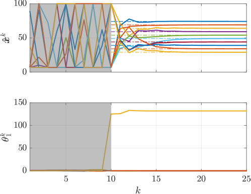
Figure 4: Nash equilibrium problem formalized in [39, Ex. 1]. The shaded regions correspond to the passive random data collection phase. Top: query points (solid lines) obtained by the external entity once solved (10) after updating the parametric estimates iteratively, converging to an equilibrium (dashed lines). Bottom: convergent behavior of the parameter vector reconstructing the BR mapping of agent $1$. Only the first 25 samples out of the allocated $K=100$ are reported in the plots.

The performance of the active learning-based approach in predicting an equilibrium solution of the considered quadratic game with no coupling constraints is illustrated in Fig. 4. In particular, the top plot shows the behaviors of the query points $\hat{\boldsymbol{x}}^{k}$ computed iteratively by the external entity to collect information on the agents’ BR mappings. Remarkably, the approximation accuracy of the BR mapping surrogates increases over the iterations, yielding $\lim_{k\to\infty}\|\hat{\boldsymbol{x}}^{k}-\boldsymbol{x}^{k}\|_{2}=0$, and therefore allowing the external entity to practically succeed in its prediction task in less than $20$ iterations. These considerations are motivated by the bottom plot in Fig. 4 that reports the convergent behavior of $\theta_{1}^{k}$ (the other parameter vectors have a similar evolution), thus supporting numerically the conditions established in Theorem 4.5.

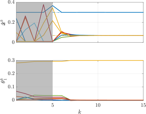
Figure 5: GNEP formalized in [40, Ex. 1]. The shaded regions correspond to the random data collection phase. Top: query points (solid lines) obtained by the external entity once solved (10) after updating the parametric estimates iteratively, converging to an equilibrium (dashed lines). Bottom: convergent behavior of the parameter vector reconstructing the BR mapping of agent $1$.

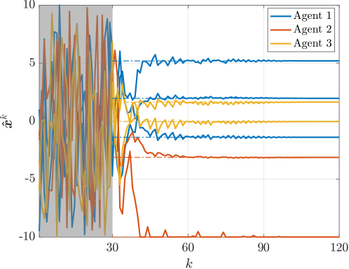
Figure 6: GNEP described in [40, Ex. 3]. The shaded region corresponds to the random data collection phase ($K_{\textrm{in}}=30$). Query points (solid lines) obtained by the external entity once solved (10) after updating the parametric estimates iteratively, converging to an equilibrium (dashed lines).

Similar conclusions can be also drawn from Fig. 5 that illustrates the case in which Algorithm 1 is applied to the example described in [40, Ex. 1] (in this case, $K=50$). Modelling the internet switching behavior induced by selfish users, in this example each cost function reads as:

$$J_{i}(x_{i},\boldsymbol{x}_{-i})=-\frac{x_{i}}{\boldsymbol{1}^{\top}_{N}\boldsymbol{x}}\left(1-\boldsymbol{1}^{\top}_{N}\boldsymbol{x}\right).$$

Then, while the first agent’s strategy is constrained so that $x_{1}\in[0.3,0.5]$, for all $j\neq 1$ we have $x_{j}\in[0.01,100]$. In addition, a standard linear constraint $\boldsymbol{1}^{\top}_{N}\boldsymbol{x}\leq 1$ couples the strategies of the whole population of decision-makers, thus actually resulting into a GNEP. An example with multidimensional decision vectors is instead the one illustrated in Fig. 6, which amounts to the GNEP described in [40, Ex. 3] and involving $N=3$ agents with three, two and two variables, respectively. Even though the point $\{\hat{\boldsymbol{x}}^{k}\}_{k\in\mathbb{N}}$ converges to is different from the GNE reported in [40, Ex. 3], it still coincides with an equilibrium of the underlying GNEP, being a fixed point of the BR mappings.

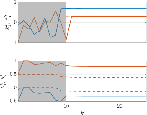
Figure 7: GNEP formalized in [40, Ex. 11]. The shaded region corresponds to the random data collection phase ($K=100$). Top: query points (solid lines) obtained by the external entity once solved (10) after updating the parametric estimates iteratively, still converging to the normalized equilibrium (dashed lines). Bottom: convergent behavior of the parameter vectors reconstructing the BR mapping for both agents (same colour, solid lines correspond to the first element of each $\theta_{i}$, while dashed lines to the second).

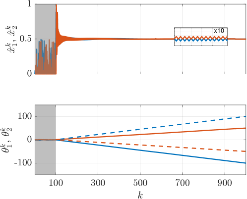
Figure 8: Nash equilibrium problem with no equilibria. The shaded region corresponds to the random data collection phase ($K_{\textrm{in}}=100$, $K=1000$). Top: query points obtained by the external entity once solved (10) after updating the parametric estimates iteratively. Bottom: diverging behavior of the parameter vectors reconstructing the BR mapping for both agents (same colour, solid lines correspond to the first element of each $\theta_{i}$, while dashed lines to the second one).

We conclude this part by discussing two simple, yet significant, examples involving two agents only. The first one consists in the GNEP in [40, Ex. 11] featuring an infinite number of equilibria $\left\{\mathrm{col}(\alpha,1-\alpha)\ \left|\ \alpha\in[1/2,1]\right.\right\}$, for which Fig. 7 shows that Algorithm 1 is actually able to return one of those solutions – specifically that coinciding with $\alpha=0.7$. On the contrary, the second example considered does not have any Nash equilibrium due to the lack of quasiconvexity in the agents’ cost functions, which are taken as $J_{1}(x_{1},x_{2})=-x_{1}^{2}+2x_{1}x_{2}$ and $J_{2}=x_{2}-2x_{1}x_{2}$, $x_{i}\in[0,1]$ for $i\in\{1,2\}$. Figure 8 reports the numerical results for this example, where it is evident the non-convergent behavior of the main quantities involved, particularly the parameter vectors $\theta_{i}$. According to the discussion in §V-A, in this case the sufficient conditions established in Theorem 4.5 do not hold, and therefore no certificate for the existence of Nash equilibria is provided, which is indeed the case. Finally, Table I shows that, in all those numerical instances considered for which convergence of the parametric estimates happens, also the sufficient condition for the uniqueness of the solution in $\mathcal{M}(\tilde{\theta})$ is met (namely, positive definiteness of the Hessian matrix $H$ of the cost function, along with convexity of $\Omega$), thus verifying the requirements in Theorem 4.5 numerically.

TABLE I: Minimum eigenvalue of the Hessian matrix of (7)

	Fig. 4	Fig. 5	Fig. 6	Fig. 7	Fig. 8
$\lambda_{\textrm{min}}(H)$	$0.11$	$0.16$	$0.001$	$0.65$	$\ast$

VI-B Multi-agent feedback controller synthesis

The control application described in §II-B is slightly more challenging, mostly because the conditions for the stack of the (highly nonlinear) action-reaction mappings (4) to admit a stationary action profile are not clear. For this reason, we selected $10$ random numerical instances on which Algorithm 1 returned a fixed point of each $f_{i}(\cdot)$ in (4) after just one execution, thus ensuring the existence of a stationary action profile according to Corollary 4.6 (Fig. 10 reports just one converging instance of the first example for agent $1$). In particular, we generated random, discrete-time LTI test models with unstable eigenvalues, satisfying the observability and reachability conditions discussed in §II-B2. Given $N=3$ agents with $n_{u_{i}}=1$ for simplicity, we have $n_{z}\sim\mathcal{U}(N,3N)$, $n_{y}\sim\mathcal{U}(N,2N)$ and $n_{y_{i}}\sim\mathcal{U}(2,n_{y})$, while weights $r_{i}\sim\mathcal{U}(1,10)$, $Q_{i}=WW^{\top}$ and $W\sim\mathcal{U}(0,1)$, $i\in\mathcal{N}$.

We started by analyzing the impact the hyperparameters have on the convergence of Algorithm 1 when applied to the first randomnly generated instance. We replicate precisely the same approach as described in the previous subsection, i.e., $K=100$, average over $20$ executions of Algorithm 1 for coefficients combination $\beta\in\{0,0.5,1,2,5\}$ and $K_{\textrm{in}}\in\{0.01,0.1,0.2,0.4\}\cdot K$. The results in Fig. 9 show that, unlike the GNEP setting, for this application the convergence rate is more sensible to the learning rate $\beta$ rather than the length of the random initialization phase (the blue lines do not even converge indeed). We thus set $\beta=2$ and $K_{\textrm{in}}=0.1K$ to conduct the numerical simulations of this subsection.

The random initialization phase is here performed by presenting to the agents centralized LQR gains obtained with output and input weights $Q=I_{n_{y}}$ and $R=I_{N}$, and after perturbing the original dynamical matrix. Moreover, to avoid the emptiness of (4) due to the unboundedness of $\kappa_{i}$, for some $\boldsymbol{\kappa}_{-i}$ the external entity computes points $\hat{\boldsymbol{\kappa}}\in\hat{\Omega}=\Omega=[-20,20]^{Nn_{z}}$.

As already spotted out in the comments following Fig. 3, from our numerical experience we have found that, given a numerical instance enjoying the existence of a stationary action profile, Algorithm 1 may not converge at each execution. With the application considered in this subsection, however, this behavior is even more pronounced, possibly also in view of the highly nonlinear structure of the underlying mappings. These considerations hence motivate us in performing a statistical analysis to shed further light on this fact, and the last column of Table II reports the percentage of convergent runs over $1000$ executions of Algorithm 1. In all the numerical simulations in which convergence of the parametric estimates happens – possibly to different points – we observe that: i) Algorithm 1 returns a fixed point of the stack of the action-reaction mappings, thus verifying numerically the theory in §IV; and, quite interestingly, ii) the point it returns is always the same. Finally, to populate the last column of Table II, for each numerical example we have taken the smallest eigenvalue of the Hessian matrix for (8) among the minimum ones $\lambda^{i}_{\textrm{min}}(H)$ in all those cases in which the convergence of the parametric estimates happened. Such a column indeed shows that the condition on $\mathcal{M}(\tilde{\theta})$ of being a singleton is always met.

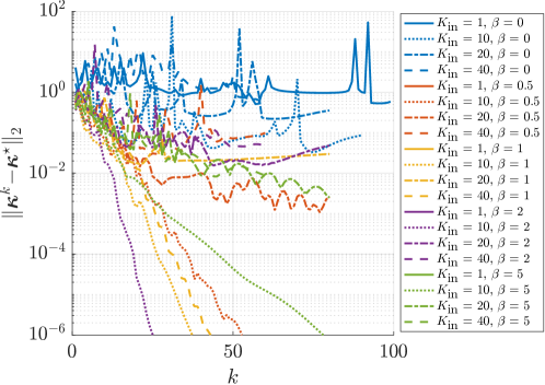
Figure 9: Hyperparameters analysis on the first randomly drawn multi-agent feedback controller synthesis problem.

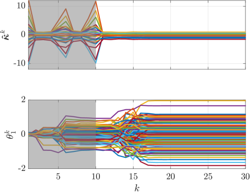
Figure 10: First randomly drawn multi-agent feedback controller synthesis problem. The shaded region corresponds to the random data collection phase ($K=100$). Top: query points obtained by the external entity once solved (10) after updating the parametric estimates, converging to a stationary action profile. Bottom: convergent behavior of the parameter vector reconstructing the action-reaction mapping (4) of agent $1$.

TABLE II: Multi-agent feedback controller synthesis – Numerical results

Example	$n_{z}$	$n_{y}$	$n_{y_{i}}$	$\%_{\textrm{conv}}$	$\underset{i}{\textrm{min}}~{}\{\lambda^{i}_{\textrm{min}}(H)\}$
$1$	$8$	$6$	$\{5,2,5\}$	$60$	$5.39\times 10^{-4}$
$2$	$7$	$4$	$\{3,2,4\}$	$49.3$	$1.23\times 10^{-3}$
$3$	$4$	$6$	$\{2,4,2\}$	$87.6$	$4.29\times 10^{-4}$
$4$	$5$	$6$	$\{4,5,5\}$	$82.5$	$1.76\times 10^{-4}$
$5$	$6$	$5$	$\{2,5,3\}$	$98.1$	$1.05\times 10^{-4}$
$6$	$4$	$6$	$\{2,3,3\}$	$89.5$	$2.59\times 10^{-4}$
$7$	$8$	$6$	$\{2,5,4\}$	$94.9$	$6.80\times 10^{-3}$
$8$	$4$	$3$	$\{3,3,2\}$	$98.6$	$1.85\times 10^{-4}$
$9$	$5$	$6$	$\{2,5,2\}$	$62.9$	$1.79\times 10^{-4}$
$10$	$8$	$5$	$\{4,5,2\}$	$94.7$	$3.54\times 10^{-3}$

VII Conclusion and outlook

We have proposed an active learning scheme allowing an external entity to reproduce faithful surrogates of action-reaction mappings, privately held by a population of interacting agents, in order to find a stationary action profile of the underlying multi-agent interaction process. We have established sufficient conditions to assess the asymptotic properties of the proposed active learning method so that, if convergence happens, it can only be towards a stationary action profile. This fact has two important consequences: i) learning locally exact surrogates of the action-reaction mappings allows the external entity to succeed in its prediction task, and ii) working with assumptions so general that a stationary profile is not even guaranteed to exist, the established conditions hence act also as certificates for the existence of such a desirable profile. We have shown the practical effectiveness of our active learning procedure numerically on a number of typical competitive multi-agent decision-making and control problems.

The proposed learning-based approach paves the way to numerous extensions in several (possibly complementary) directions. Looking at the specific problem of learning a GNE in GNEPs, for instance, given the tight connection between an equilibrium solution and a minimizer of the so-called Nikaido-Isoda function [42], one may design a tailored procedure along the line of Algorithm 1 to locally approximate such a function. According to the discussion in §V-C, investigating conditions under which also family of surrogate mappings different from the affine one may lead to the same asymptotic properties for our active learning procedure is a challenging problem. In addition, one may consider the case in which $\Omega$ is not known by also learning an appropriate surrogate set $\hat{\Omega}$ of $\Omega$ during the execution of Algorithm 1. Finally, we remark that problem (7) is based completely on exploiting the current predictors $\hat{f}_{i}$. In alternative to the initial random exploration phase, one could also investigate possible solution for better exploring the decision set $\Omega$, as typically done for example in reinforcement learning  [43] and surrogate-based global optimization [44], and analyze its potential benefits.

Appendix A Appendix

A-A Technical proofs

Proof of Lemma 3.3: Let $\bar{f}:\mathbb{R}^{n}\times\mathbb{R}^{p}\to\bar{\mathbb{R}}$ be defined by $\bar{f}(x,\theta)\coloneqq f(x,\theta)+\iota_{\mathcal{X}}(x)$. Since $\mathcal{X}$ is a convex set and $f$ is a convex function, then $\bar{f}$ is also a convex function for each given $\theta\in\mathbb{R}^{p}$. By applying [30, Th. 2.6], it follows that $\mathcal{M}(\theta)=\textrm{argmin}_{y\in\mathbb{R}^{n}}~{}\bar{f}(y,\theta)$ is a convex set for all $\theta\in\mathbb{R}^{p}$.

To show continuity of $f^{\star}$ at a generic $\tilde{\theta}\in\mathbb{R}^{p}$, we need to prove that $\lim_{k\rightarrow\infty}f^{\star}(\theta^{k})=f^{\star}(\tilde{\theta}),$ for any sequence $\{\theta^{k}\}_{k\in\mathbb{N}}$ such that $\lim_{k\rightarrow\infty}\theta^{k}=\tilde{\theta}$. Consider such a generic sequence and let $x^{k}\in\mathcal{M}(\theta^{k})$ and $\tilde{x}\in\mathcal{M}(\tilde{\theta})$. In view of Assumption 3.2, $\theta\mapsto f(x^{k},\theta)$ is also convex and differentiable w.r.t. $\theta$ and $\tilde{x}\in\mathcal{M}(\tilde{\theta})$, i.e., $\tilde{x}$ is a global minimizer of $f(\cdot,\tilde{\theta})$, and therefore we have that

$$\begin{split}f^{\star}(\theta^{k})=f(x^{k},\theta^{k})&\geq f(x^{k},\tilde{\theta})+\frac{\partial f(x^{k},\theta)}{\partial\theta}\Big{\rvert}_{\theta=\tilde{\theta}}^{\top}(\theta^{k}-\tilde{\theta})\\ &\geq f(\tilde{x},\tilde{\theta})+\frac{\partial f(x^{k},\tilde{\theta})}{\partial\theta}\Big{\rvert}_{\theta=\tilde{\theta}}^{\top}(\theta^{k}-\tilde{\theta})\\ &\geq f(\tilde{x},\tilde{\theta})-D(\tilde{\theta})\|\theta^{k}-\tilde{\theta}\|,\end{split}$$

where the last inequality holds since the partial derivative $\partial f(x,\theta)/\partial\theta$ evaluated in $\tilde{\theta}$ is bounded w.r.t. $x$, with bound $D(\tilde{\theta})\coloneqq\textrm{sup}_{x\in\mathcal{X}}\left|\tfrac{\partial f(x,\theta)}{\partial\theta}\Big{\rvert}_{\theta=\tilde{\theta}}\right|\in\mathbb{R}$. Therefore, we obtain:

$$f(\tilde{x},\tilde{\theta})-D(\tilde{\theta})\|\theta^{k}-\tilde{\theta}\|\leq f^{\star}(\theta^{k})=f(x^{k},\theta^{k})\leq f(\tilde{x},\theta^{k})$$ (14)

where the last inequality follows by the optimality of $x^{k}$. Since $\theta\mapsto f(x,\theta)$ is continuous and $\lim_{k\rightarrow\infty}\theta^{k}=\tilde{\theta}$, we have that $\lim_{k\rightarrow\infty}f(\tilde{x},\theta^{k})=f(\tilde{x},\tilde{\theta})$, and the proof concludes by applying the squeeze theorem to (14). $\blacksquare$

Proof of Lemma 3.6: Lower semicontinuity of $\bar{f}(x,\theta)$ readily follows by the continuity of $f(x,\theta)$ at any given point $(\tilde{x},\tilde{\theta})\in\mathbb{R}^{n}\times\mathbb{R}^{p}$, as

$$\lim_{(x,\theta)\rightarrow(\tilde{x},\tilde{\theta})}\inf\bar{f}(x,\theta) =\lim_{\varepsilon\rightarrow 0}\left[\inf_{(y,\xi)\in\mathcal{B}_{\varepsilon}(\tilde{x},\tilde{\theta})}f(y,\xi)\right]$$

$$=\left\{\begin{array}[]{lll}f(\tilde{x},\tilde{\theta})&\mbox{if}&\tilde{x}\in\mathcal{X}\\ +\infty&\mbox{if}&\tilde{x}\not\in\mathcal{X}\end{array}\right.$$

which in turn implies that $\lim_{(x,\theta)\rightarrow(\tilde{x},\tilde{\theta})}\inf\bar{f}(x,\theta)\geq\bar{f}(\tilde{x},\tilde{\theta})$ for all $(\tilde{x},\tilde{\theta})\in\mathbb{R}^{n}\times\mathbb{R}^{p}$. To show level-boundedness, note that $\mathcal{X}$ is bounded and nonempty, and therefore, for all $\alpha\in\mathbb{R}$, $\left\{x\in\mathbb{R}^{n}\ \left|\ \bar{f}(x,\theta)\leq\alpha\right.\right\}\subseteq\mathcal{X}$ for all $\theta\in\mathbb{R}^{p}$. Thus, by setting $\mathcal{S}=\mathcal{X}$ and $g=\bar{f}$ in Definition 3.5, the claim follows. $\blacksquare$

Proof of Lemma 3.7: By [30, Th. 2.6], each vector $x^{k}$ in (5) is uniquely defined since $\tfrac{1}{2}\|\cdot\|_{2}^{2}$ is strictly convex, proper because $\mathcal{X}$ is nonempty and therefore, by Lemma 3.3, $\mathcal{M}(\theta^{k})$ is a convex set. Moreover, since $x\mapsto f(x,\theta)$ is continuous for all $\theta\in\mathbb{R}^{p}$ and $\mathcal{X}$ is compact, by Lemma 3.6 the function $\bar{f}(x,\theta)$, defined by $\bar{f}(x,\theta)=f(x,\theta)+\iota_{\mathcal{X}}(x)$, is lower semicontinuous w.r.t. $x$ and level-bounded in $x$ locally uniformly w.r.t. $\theta$. Still in view of Lemma 3.3, we also have that $\lim_{k\rightarrow\infty}f^{\star}(\theta^{k})=f^{\star}(\tilde{\theta})$. Thus, from [30, Th. 1.17(b)] it follows that the sequence $\{x^{k}\}_{k\in\mathbb{N}}$ generated by (5) is bounded and all its cluster points lie in $\mathcal{M}(\tilde{\theta})$, which is however a singleton and contains $\tilde{x}$ only.

For the sake of contradiction, assume that $x^{k}\not\rightarrow\tilde{x}$ as $k\rightarrow\infty$. Then, there exists some $\varepsilon>0$ and an infinite subsequence $\{x^{k}\}_{k\in\mathcal{I}}$ so that $\|x^{k}-\tilde{x}\|_{2}>\varepsilon$ for all $k\in\mathcal{I}$. Since $\{x^{k}\}_{k\in\mathcal{I}}$ is also bounded, by the Bolzano-Weierstrass theorem there exists an infinite subsequence $\{x^{k}\}_{k\in\mathcal{I}^{\prime}}$, with $\mathcal{I}^{\prime}\subset\mathcal{I}$, such that $\lim_{k\rightarrow\infty,k\in\mathcal{I}^{\prime}}x^{k}=\bar{x}$, with $\bar{x}\neq\tilde{x}$. Since $\bar{x}$ is a cluster point of $\{x^{k}\}_{k\in\mathbb{N}}$, by relying on [30, Th. 1.17(b)] we have that $\bar{x}\in\mathcal{M}(\tilde{\theta})$. This however is in conflict with the fact that $\mathcal{M}(\tilde{\theta})$ is a singleton, i.e., $\mathcal{M}(\tilde{\theta})=\{\tilde{x}\}$, and hence the assumption $x^{k}\not\rightarrow\tilde{x}$ for $k\rightarrow\infty$ is contradicted, proving the statement. $\blacksquare$

Proof of Lemma 4.2: Let us consider a single agent $i\in\mathcal{N}$, as the proof for the remaining ones is identical mutatis mutandis. By making use of a contradiction argument, we will show that any of the parameters $\bar{\theta}_{i}\in\mathcal{A}_{i}\coloneqq\mathcal{A}_{i}(\bar{x}_{i},\bar{\boldsymbol{x}}_{-i})$ asymptotically belongs to the set of minimizers of $\xi_{i}\mapsto\frac{1}{k}\sum_{t=1}^{k}\ell_{i}(x_{i}^{t},\hat{f}_{i}(\hat{\boldsymbol{x}}^{t}_{-i},\xi_{i}))$, and therefore it shall happen that $\bar{\theta}_{i}\in\mathcal{A}_{i}$. Recall, indeed, that the parameter update reads as $\theta_{i}^{k+1}=\textrm{argmin}_{\xi_{i}\in\mathbb{R}^{p_{i}}}\,\frac{1}{k}\sum_{t=1}^{k}\ell_{i}(x_{i}^{t},\hat{f}_{i}(\hat{\boldsymbol{x}}^{t}_{-i},\xi_{i}))$, where equality follows by virtue of the global optimality assumed and the tie-break rule $\mathcal{T}(\cdot)$ in place. Thus, for the sake of contradiction, let us assume that $\lim_{k\to\infty}\theta_{i}^{k}=\tilde{\theta}_{i}$ with $\tilde{\theta}_{i}\notin\mathcal{A}_{i}$.

To start we note that, by combining the definition of limit [45, Def. 5.4] and the properties of the loss function stated in Standing Assumption 4.1, along with those of the affine surrogates $\hat{f}_{i}$ described in §IV-B, $\lim_{k\to\infty}x_{i}^{k}=\bar{x}_{i}$ and $\lim_{k\to\infty}\hat{\boldsymbol{x}}^{k}_{-i}=\bar{\boldsymbol{x}}_{-i}$ so that $(\bar{x}_{i},\bar{\boldsymbol{x}}_{-i})\in\Omega$ directly imply that $\lim_{k\to\infty}\ell_{i}(x_{i}^{k},\hat{f}_{i}(\hat{\boldsymbol{x}}^{k}_{-i},\tilde{\theta}_{i}))=v>0$, for any $\tilde{\theta}_{i}\notin\mathcal{A}_{i}$, while for all $\tilde{\theta}_{i}\in\mathcal{A}_{i}$ instead, $\lim_{k\to\infty}\ell_{i}(x_{i}^{k},\hat{f}_{i}(\hat{\boldsymbol{x}}^{k}_{-i},\tilde{\theta}_{i}))=0$. Since we are assuming that $\lim_{k\to\infty}\theta_{i}^{k}=\tilde{\theta}_{i}$, by considering a generic $\theta_{i}^{k}$ obtained from (6) we know that for any $\tilde{\varepsilon}>0$ there exists some $\tilde{M}\coloneqq\tilde{M}(\tilde{\varepsilon})\geq 0$ so that $|\ell_{i}(x_{i}^{k},\hat{f}_{i}(\hat{\boldsymbol{x}}^{k}_{-i},\theta^{k}_{i}))-v|\leq\tilde{\varepsilon}$, i.e., $-\tilde{\varepsilon}+v\leq\ell_{i}(x_{i}^{k},\hat{f}_{i}(\hat{\boldsymbol{x}}^{k}_{-i},\theta^{k}_{i}))\leq\tilde{\varepsilon}+v$, for all $k\geq\tilde{M}$. On the other hand, we also know from $\lim_{k\to\infty}\ell_{i}(x_{i}^{k},\hat{f}_{i}(\hat{\boldsymbol{x}}^{k}_{-i},\tilde{\theta}_{i}))=0$ that for any $\bar{\varepsilon}>0$ there exists some $\bar{M}\coloneqq\bar{M}(\bar{\varepsilon})\geq 0$ so that $\ell_{i}(x_{i}^{k},\hat{f}_{i}(\hat{\boldsymbol{x}}^{k}_{-i},\tilde{\theta}_{i}))\leq\bar{\varepsilon}$ for all $k\geq\bar{M}$.

Without loss of generality, let us then pick $\tilde{\varepsilon}=v/2$ so that $-\ell_{i}(x_{i}^{k},\hat{f}_{i}(\hat{\boldsymbol{x}}^{k}_{-i},\theta^{k}_{i}))\leq-v/2$, and fix $\bar{\varepsilon}<\tilde{\varepsilon}=v/2$, which is always possible by continuity and $k$ sufficiently large. Under this latter condition, precisely $k>\textrm{max}\{\tilde{M},\bar{M}\}$, evaluating the summation of the difference of the loss functions in $\bar{\theta}_{i}$ and $\theta^{k}_{i}$ at iteration $k$, with each term $\Delta\ell_{i,k}^{t}\coloneqq\ell_{i}(x_{i}^{t},\hat{f}_{i}(\hat{\boldsymbol{x}}^{t}_{-i},\tilde{\theta}_{i}))-\ell_{i}(x_{i}^{t},\hat{f}_{i}(\hat{\boldsymbol{x}}^{t}_{-i},\theta^{k}_{i}))$, leads to:

$$\frac{1}{k}\sum_{t=1}^{k}\Delta\ell_{i,k}^{t}=\frac{1}{k}\left[\sum_{t=1}^{\textrm{min}\{\tilde{M},\bar{M}\}-1}\Delta\ell_{i,k}^{t}+\sum_{t=\textrm{min}\{\tilde{M},\bar{M}\}}^{\textrm{max}\{\tilde{M},\bar{M}\}-1}\Delta\ell_{i,k}^{t}+\sum_{t=\textrm{max}\{\tilde{M},\bar{M}\}}^{k}\Delta\ell_{i,k}^{t}\right].$$

While the first term in the summation is constant for fixed $\bar{\varepsilon}$ and $\tilde{\varepsilon}$ (and therefore for fixed $\bar{M}$ and $\tilde{M}$), namely $\sum_{t=1}^{\textrm{min}\{\tilde{M},\bar{M}\}-1}\Delta\ell_{i,k}^{t}\eqqcolon\alpha$, the second and third elements can always be upper bounded by $(k-\bar{\rho})\bar{\varepsilon}-(k-\tilde{\rho})v/2+\beta$, where $\bar{\rho}$, $\tilde{\rho}\geq 0$ and $\beta\in\mathbb{R}$ are constants depending on the values $\tilde{M}$ and $\bar{M}$ take. Specifically, if $\bar{M}<\tilde{M}$, $\bar{\rho}=\bar{M}$, $\tilde{\rho}=\tilde{M}$ and $\beta<0$, whereas if $\bar{M}\geq\tilde{M}$, $\bar{\rho}=\tilde{M}$, $\tilde{\rho}=\bar{M}$ and $\beta>0$. Thus, taking the limit for $k\to\infty$ yields inequality:

$$\lim\limits_{k\to\infty}\frac{1}{k}\sum_{t=1}^{k}\Delta\ell_{i,k}^{t}\leq\lim\limits_{k\to\infty}\frac{1}{k}[\alpha+\beta+(k-\bar{\rho})\bar{\varepsilon}-(k-\tilde{\rho})v/2]<0$$

in view of $\bar{\varepsilon}<\tilde{\varepsilon}=v/2$, meaning that we can always find some iteration index such that the cost obtained with some $\tilde{\theta}_{i}\in\mathcal{A}_{i}$ is strictly smaller than the one obtained with $\theta^{k}_{i}$ updated through the rule in (6), and assumed to be convergent to some $\tilde{\theta}_{i}\notin\mathcal{A}_{i}$. This clearly represents a contradiction and hence concludes the proof. $\blacksquare$

Proof of Proposition 4.4: Let us prove that $f(\boldsymbol{x},\theta)=\sum_{i\in\mathcal{N}}\|x_{i}-(\nu^{k+1}_{i})^{\top}\boldsymbol{x}_{-i}-c^{k+1}_{i}\|^{2}_{2}$ satisfies Assumption 3.1 and 3.2. Since $\Omega$ is a nonempty polytope, it is convex and bounded. Moreover, function $f$ is quadratic and positive semidefinite, and therefore continuous and convex w.r.t. $\boldsymbol{x}$, for all $\theta\in\mathbb{R}^{p}$. In addition, $f(\boldsymbol{x},\theta)$ can be expressed also as:

$$f(\boldsymbol{x},\theta) =\|A(\boldsymbol{x})\theta-b(\boldsymbol{x})\|_{2}^{2}$$

$$=\theta^{\top}A(\boldsymbol{x})^{\top}A(\boldsymbol{x})\theta+2b(\boldsymbol{x})^{\top}A(\boldsymbol{x})\theta+b(\boldsymbol{x})^{\top}b(\boldsymbol{x})$$

where $A(\boldsymbol{x})$, $b(\boldsymbol{x})$ are suitably defined affine functions of $\boldsymbol{x}$, which is a quadratic positive semidefinite function w.r.t. to $\theta$, and therefore convex and differentiable for all $\boldsymbol{x}\in\Omega$. Thus,

$$\begin{split}\underset{\boldsymbol{x}\in\Omega}{\textrm{sup}}~{}\left|\frac{\partial f(\boldsymbol{x},\theta)}{\partial\theta}\right|&=\underset{\boldsymbol{x}\in\Omega}{\textrm{max}}~{}\left|2A(\boldsymbol{x})^{\top}A(\boldsymbol{x})\theta+A(\boldsymbol{x})^{\top}b(\boldsymbol{x})\right|\\ &=\underset{i=1,\ldots,q}{\textrm{max}}~{}\pm\{2A(v_{i})^{\top}A(v_{i})\theta+A(v_{i})^{\top}b(v_{i})\}\end{split}$$

where $v_{1},\ldots,v_{q}$ are the vertices of $\Omega$ and the last inequality follows since $2A(\boldsymbol{x})^{\top}A(\boldsymbol{x})\theta+A(\boldsymbol{x})^{\top}b(\boldsymbol{x})$ is convex and quadratic w.r.t. $\boldsymbol{x}$ and the maximum of a convex quadratic function over a polytope is attained at one of its vertices. For all $\theta\in\mathbb{R}^{p}$, we thus obtain that:

$$\begin{split}&\underset{\boldsymbol{x}\in\Omega}{\textrm{max}}~{}\left|2A(\boldsymbol{x})^{\top}A(\boldsymbol{x})\theta+A(\boldsymbol{x})^{\top}b(\boldsymbol{x})\right|\\ &=\max\{2A(v_{i(\theta)})^{\top}A(v_{i(\theta)})\theta+A(v_{i(\theta)})^{\top}b(v_{i(\theta)}),\\ &~{}~{}~{}~{}~{}~{}~{}~{}-2A(v_{j(\theta)})^{\top}A(v_{j(\theta)})\theta+A(v_{j(\theta)})^{\top}b(v_{j(\theta)})\}\eqqcolon D(\theta)\end{split}$$

for some indices ${i(\theta)}$, ${j(\theta)}\in\{1,\ldots,q\}$. By relying on Lemma 3.7 we hence obtain the desired result, since all its assumptions are satisfied. $\blacksquare$

Proof of Theorem 4.5: The convergence of each $\theta_{i}^{k}$ to some $\tilde{\theta}_{i}$ clearly implies that, in view of Standing Assumption 4.1, also the associated composition mapping estimate converges, i.e., for all $i\in\mathcal{N}$, $\lim_{k\to\infty}\hat{f}_{i}(\boldsymbol{x}_{-i},\theta^{k}_{i})=\hat{f}_{i}(\boldsymbol{x}_{-i},\tilde{\theta}_{i})$ with $\hat{f}_{i}(\boldsymbol{x}_{-i},\tilde{\theta}_{i})$ possibly different from the true action-reaction mapping $f_{i}(\boldsymbol{x}_{-i})$. Then, in view of Proposition 4.4, we also have that $\lim_{k\to\infty}\hat{\boldsymbol{x}}^{k}=\tilde{\boldsymbol{x}}$. This latter relation in turn yields $\lim_{k\to\infty}\boldsymbol{x}^{k}=\bar{\boldsymbol{x}}$, as the action-reaction mappings $f_{i}(\cdot)$ are single-valued and continuous in view of Standing Assumption 2.2. Note that both sequences $\{\hat{\boldsymbol{x}}^{k}\}_{k\in\mathbb{N}}$ and $\{\boldsymbol{x}^{k}\}_{k\in\mathbb{N}}$ are feasible in view of (7) and the fact that each $x_{i}^{k}$ is determined through $f_{i}(\cdot)$ that implicitly accounts for the common constraints $\Omega$. Since $\hat{\boldsymbol{x}}^{k}$ is iteratively chosen following the tie-break rule induced by $\tfrac{1}{2}\|\cdot\|_{2}^{2}$, as the set of global minimizers in (7) may not be unique, it may happen that $\tilde{\boldsymbol{x}}\neq\bar{\boldsymbol{x}}$. We now make use of a local exact approximation argument to show that $\lim_{k\to\infty}\|\hat{\boldsymbol{x}}^{k}-\boldsymbol{x}^{k}\|_{2}=0$, and hence that the two limit points above coincide, and actually yield, by virtue of Lemma 4.2, a stationary action profile $\boldsymbol{x}^{\star}$ in the sense of Definition 2.1.

In view of the definition of limit we can then always find some $\bar{k}\in\mathbb{N}$ and $\mu_{i}>0$ such that a neighbourhood of $\bar{x}_{i}$, say $\mathcal{B}_{\mu_{i}}(\bar{x}_{i})$, contains infinitely many points [46], meaning that $x_{i}^{k}\in\mathcal{B}_{\mu_{i}}(\bar{x}_{i})$ for all $k\geq\bar{k}$, $i\in\mathcal{N}$. By virtue of the consistency property proved in Lemma 4.2 it thus follows that the pointwise approximation shall be exact, namely each $\tilde{\theta}_{i}$ is so that $\|\hat{f}_{i}(\bar{\boldsymbol{x}}_{-i},\tilde{\theta}_{i})-f_{i}(\bar{\boldsymbol{x}}_{-i})\|_{2}=0$, i.e., $\tilde{\theta}_{i}\in\mathcal{A}_{i}=\mathcal{A}_{i}(\tilde{x}_{i},\bar{\boldsymbol{x}}_{i})$.

This latter relation has hence two main consequences. First, it excludes the possibility that, due to the presence of some tie-break rule $\mathcal{T}(\cdot)$, $\lim_{k\to\infty}\|\hat{\boldsymbol{x}}^{k}-\boldsymbol{x}^{k}\|_{2}\neq 0$, namely the external entity can not learn any map but the true one locally, thus forcing $\tilde{\boldsymbol{x}}=\bar{\boldsymbol{x}}$. If this were not the case, indeed, the update rule for each $\theta_{i}$ would be fed with different samples, thus possibly preventing their convergence (this would also happen if a tie-break rule for singling out a minimizer from (6) were not adopted). Furthermore, in view of Definition 2.1 and since (7) is solved at the global optimum at every $k\in\mathbb{N}$, it shall happen that $\sum_{i\in\mathcal{N}}\|\hat{\boldsymbol{x}}_{i}-\hat{f}_{i}(\hat{\boldsymbol{x}}_{-i},\tilde{\theta}_{i})\|^{2}_{2}=\sum_{i\in\mathcal{N}}\|\hat{\boldsymbol{x}}_{i}-f_{i}(\hat{\boldsymbol{x}}_{-i})\|^{2}_{2}=0=\sum_{i\in\mathcal{N}}\|\bar{\boldsymbol{x}}_{i}-f_{i}(\bar{\boldsymbol{x}}_{-i})\|^{2}_{2}$, and hence $\|\bar{\boldsymbol{x}}_{i}-f_{i}(\bar{\boldsymbol{x}}_{-i})\|_{2}=0$ for all $i\in\mathcal{N}$. This latter $\bar{\boldsymbol{x}}\in\Omega$ therefore coincides with a fixed point of the action-reaction mappings $f_{i}(\cdot)$, and hence with a stationary action profile in the sense of Definition 2.1, concluding the proof. $\blacksquare$

A-B Derivation of Kalman filter equations in (13)

The updates (13) are obtained by applying linear Kalman filtering to the following linear time-varying system (we omit the index $i$ for simplicity of notation):

$$\begin{array}[]{rcl}\theta^{k+1}&=&\theta^{k}+\xi^{k}\\ x^{k}&=&(\phi^{k})^{\top}\theta^{k}+\zeta^{k},\end{array}$$

where $\xi^{k}$, $\zeta^{k}$ are zero-mean white noise terms with covariance $\beta I$ and 1, respectively. The Kalman filter equations are:

$$\begin{array}[]{rcl}M^{k}&=&P^{k}\phi^{k}/(1+(\phi^{k})^{\top}P^{k}\phi^{k})\\ \theta^{k+\nicefrac{{1}}{{2}}}&=&\theta^{k}+M^{k}(x^{k}-(\phi^{k})^{\top}\theta^{k})\\ P^{k+\nicefrac{{1}}{{2}}}&=&(I-M^{k}(\phi^{k})^{\top})P^{k}\\ &=&P^{k}-P^{k}\phi^{k}(\phi^{k})^{\top}P^{k}/(1+(\phi^{k})^{\top}P^{k}\phi^{k})\\ \theta^{k+1}&=&\theta^{k+\nicefrac{{1}}{{2}}}\\ P^{k+1}&=&P^{k+\nicefrac{{1}}{{2}}}+\beta I.\end{array}$$

Since

$$P^{k+\nicefrac{{1}}{{2}}}\phi^{k}=P^{k}\phi^{k}-P^{k}\phi^{k}(\phi^{k})^{\top}P^{k}\phi^{k}/(1+(\phi^{k})^{\top}P^{k}\phi^{k})$$

$$~{}~{}~{}~{}~{}=P^{k}\phi^{k}-P^{k}\phi^{k}(1+(\phi^{k})^{\top}P^{k}\phi^{k}-1)/(1+(\phi^{k})^{\top}P^{k}\phi^{k})$$

$$~{}~{}~{}~{}~{}=P^{k}\phi^{k}/(1+(\phi^{k})^{\top}P^{k}\phi^{k})=M^{k},$$

we finally obtain $\theta^{k+1}=\theta^{k}+P^{k}\phi^{k}/(1+(\phi^{k})^{\top}P^{k}\phi^{k})(x^{k}-(\phi^{k})^{\top}\theta^{k})$.

References

- [1] F. Fabiani and P. J. Goulart, “Reliably-stabilizing piecewise-affine neural network controllers,” IEEE Transactions on Automatic Control, pp. 1–15, 2022.
- [2] W. Jongeneel, T. Sutter, and D. Kuhn, “Efficient learning of a linear dynamical system with stability guarantees,” IEEE Transactions on Automatic Control, vol. 68, no. 5, pp. 2790–2804, 2023.
- [3] A. Bemporad and D. Piga, “Global optimization based on active preference learning with radial basis functions,” Machine Learning, vol. 110, no. 2, pp. 417–448, 2021.
- [4] D. Masti and A. Bemporad, “Learning nonlinear state–space models using autoencoders,” Automatica, vol. 129, p. 109666, 2021.
- [5] L. Ljung, “Perspectives on system identification,” Annual Reviews in Control, vol. 34, no. 1, pp. 1–12, 2010.
- [6] G. Pillonetto, F. Dinuzzo, T. Chen, G. De Nicolao, and L. Ljung, “Kernel methods in system identification, machine learning and function estimation: A survey,” Automatica, vol. 50, no. 3, pp. 657–682, 2014.
- [7] A. Bemporad, “A piecewise linear regression and classification algorithm with application to learning and model predictive control of hybrid systems,” IEEE Transactions on Automatic Control, vol. 68, no. 6, pp. 3194–3209, 2023, (Code available at http://cse.lab.imtlucca.it/ bemporad/parc).
- [8] K. J. Aström, P. Albertos, M. Blanke, A. Isidori, W. Schaufelberger, and R. Sanz, Control of complex systems. Springer Science & Business Media, 2011.
- [9] F. Facchinei and C. Kanzow, “Generalized Nash equilibrium problems,” Annals of Operations Research, vol. 175, no. 1, pp. 177–211, 2010.
- [10] J. Fearnley, M. Gairing, P. Goldberg, and R. Savani, “Learning equilibria of games via payoff queries,” in Proceedings of the fourteenth ACM conference on Electronic commerce, 2013, pp. 397–414.
- [11] Y. Babichenko, “Query complexity of approximate Nash equilibria,” Journal of the ACM (JACM), vol. 63, no. 4, pp. 1–24, 2016.
- [12] P. W. Goldberg and A. Roth, “Bounds for the query complexity of approximate equilibria,” ACM Transactions on Economics and Computation (TEAC), vol. 4, no. 4, pp. 1–25, 2016.
- [13] Y. Babichenko and A. Rubinstein, “Communication complexity of approximate Nash equilibria,” in Proceedings of the 49th Annual ACM SIGACT Symposium on Theory of Computing, 2017, pp. 878–889.
- [14] S. Hart and N. Nisan, “The query complexity of correlated equilibria,” Games and Economic Behavior, vol. 108, pp. 401–410, 2018.
- [15] P. W. Goldberg and F. J. Marmolejo-Cossío, “Learning convex partitions and computing game-theoretic equilibria from best-response queries,” ACM Transactions on Economics and Computation (TEAC), vol. 9, no. 1, pp. 1–36, 2021.
- [16] E. A. Viqueira and C. Cousins, “Learning simulation-based games from data,” in Proceeding AAMAS’19 Proceedings of the 18th International Conference on Autonomous Agents and Multi-Agent Systems, vol. 2019, 2019.
- [17] E. A. Viqueira, C. Cousins, and A. Greenwald, “Improved algorithms for learning equilibria in simulation-based games,” in Proceedings of the 19th International Conference on Autonomous Agents and Multi-Agent Systems, 2020, pp. 79–87.
- [18] A. Marchesi, F. Trovò, and N. Gatti, “Learning probably approximately correct maximin strategies in simulation-based games with infinite strategy spaces,” in Proceedings of the 19th International Conference on Autonomous Agents and Multi-Agent Systems, 2020, pp. 834–842.
- [19] Y. Vorobeychik and M. P. Wellman, “Stochastic search methods for Nash equilibrium approximation in simulation-based games,” in Proceedings of the 7th International Conference on Autonomous Agents and Multi-Agent Systems, 2008, pp. 1055–1062.
- [20] Y. Vorobeychik, “Probabilistic analysis of simulation-based games,” ACM Transactions on Modeling and Computer Simulation (TOMACS), vol. 20, no. 3, pp. 1–25, 2010.
- [21] A. Al-Dujaili, E. Hemberg, and U. M. O’Reilly, “Approximating Nash equilibria for black-box games: A bayesian optimization approach,” arXiv preprint arXiv:1804.10586, 2018.
- [22] V. Picheny, M. Binois, and A. Habbal, “A Bayesian optimization approach to find Nash equilibria,” Journal of Global Optimization, vol. 73, no. 1, pp. 171–192, 2019.
- [23] S. Clarke, G. Dragotto, J. F. Fisac, and B. Stellato, “Learning rationality in potential games,” arXiv preprint arXiv:2303.11188, 2023.
- [24] Y. Vorobeychik, M. P. Wellman, and S. Singh, “Learning payoff functions in infinite games,” Machine Learning, vol. 67, no. 1, pp. 145–168, 2007.
- [25] Y. Huang and J. Hu, “Distributed stochastic Nash equilibrium learning in locally coupled network games with unknown parameters,” in Learning for Dynamics and Control Conference. PMLR, 2022, pp. 342–354.
- [26] F. Fabiani, A. Simonetto, and P. J. Goulart, “Learning equilibria with personalized incentives in a class of nonmonotone games,” in 2022 European Control Conference (ECC), 2022, pp. 2179–2184.
- [27] ——, “Personalized incentives as feedback design in generalized Nash equilibrium problems,” IEEE Transactions on Automatic Control, pp. 1–16, 2023.
- [28] C. A. R. Crusius and A. Trofino, “Sufficient LMI conditions for output feedback control problems,” IEEE Transactions on Automatic Control, vol. 44, no. 5, pp. 1053–1057, 1999.
- [29] D. Barcelli, D. Bernardini, and A. Bemporad, “Synthesis of networked switching linear decentralized controllers,” in 49th IEEE Conference on Decision and Control (CDC). IEEE, 2010, pp. 2480–2485.
- [30] R. T. Rockafellar and R. J.-B. Wets, Variational analysis. Springer Science & Business Media, 2009, vol. 317.
- [31] L. Ljung and T. Söderström, Theory and practice of recursive identification. MIT press, 1983.
- [32] T. Kailath, A. H. Sayed, and B. Hassibi, Linear estimation. Prentice-Hall, 2000.
- [33] S. T. Alexander and A. L. Ghirnikar, “A method for recursive least squares filtering based upon an inverse QR decomposition,” IEEE Transactions on Signal Processing, vol. 41, no. 1, pp. 20–30, 1993.
- [34] R. E. Kalman, “A new approach to linear filtering and prediction problems,” Journal of basic Engineering, vol. 82, no. 1, pp. 35–45, 1960.
- [35] A. Bemporad, “Recurrent neural network training with convex loss and regularization functions by extended Kalman filtering,” IEEE Transactions on Automatic Control, pp. 1–8, 2022.
- [36] B. Settles, “Active learning,” in Synthesis Lectures on Artificial Intelligence and Machine Learning. Morgan & Claypool Publishers, 2012, no. 18.
- [37] P. Kumar and A. Gupta, “Active learning query strategies for classification, regression, and clustering: A survey,” Journal of Computer Science and Technology, vol. 35, no. 4, pp. 913–945, 2020.
- [38] A. Bemporad, “Active learning for regression by inverse distance weighting,” Information Sciences, vol. 626, pp. 275–292, 2023.
- [39] F. Salehisadaghiani, W. Shi, and L. Pavel, “An ADMM approach to the problem of distributed Nash equilibrium seeking.” CoRR, 2017.
- [40] F. Facchinei and C. Kanzow, “Penalty methods for the solution of generalized Nash equilibrium problems (with complete test problems),” Institute of Mathematics, University of Würzburg, Würzburg, Tech. Rep., 2009.
- [41] M. V. Solodov and P. Tseng, “Modified projection-type methods for monotone variational inequalities,” SIAM Journal on Control and Optimization, vol. 34, no. 5, pp. 1814–1830, 1996.
- [42] H. Nikaidô and K. Isoda, “Note on non-cooperative convex games,” Pacific Journal of Mathematics, vol. 5, no. S1, pp. 807–815, 1955.
- [43] R. S. Sutton and A. G. Barto, Reinforcement learning: An introduction. MIT press, 2018.
- [44] A. Bemporad, “Global optimization via inverse distance weighting and radial basis functions,” Computational Optimization and Applications, vol. 77, pp. 571–595, 2020, (Code available at http://cse.lab.imtlucca.it/ bemporad/glis).
- [45] B. S. Thomson, J. B. Bruckner, and A. M. Bruckner, Elementary real analysis. Prentice-Hall, 2001.
- [46] G. Bachman and L. Narici, Functional analysis. Courier Corporation, 2000.