Effects of quantum geometric phase of a particle in an oscillating hard-wall spherical trap

Abstract

We obtain the geometric phase for states of a particle in a spherical infinite potential well with moving walls in two different cases; First, when the radius of the well increases (or decreases) monotonically. Second, when the radius changes oscillatory. In the latter case, we have solved the Schrödinger equation and found its solutions approximately. We obtain the transition rate for the possible real situation in an acousto-optic case which can reveal the effect of the geometric phase. We show that the absorption or radiation peaks will appear if the energy gap between the incident photon and the modified energy difference of two levels by the geometric phase, is equal to the integer multiple of oscillation frequency.

I Introduction

The Berry phase is a gauge invariant and geometrical phase which is firstly defined by Berry in 1984 Berry1984 . As a matter of fact, many physical situations are contained of objects whose behavior is specified up to a phase by certain parameters. Berry phase appears when the transversal of a closed path by the parameters, which at the end of the path they have returned to their initial values, leads to a change of phase whose magnitude depends only on the path (For a collection of papers on the subject, see wilczek ).

As a simple example consider a magnet precessing about a magnetic field. Here the parameters are the three components of the field. The field is slowly rotated and finally, returns to its original direction. In this situation, the phase angle of the precession will be shifted from what it would be if the field had been held constant Cina1986 . In addition, recently many works have been published on the Berry phase and its applications in various fields. For example, in Ref. marija a system of strongly interacting one-dimensional (1D) bosons on a ring pierced by a synthetic magnetic flux tube is studied. In Ref. Antti , Employing the spectral interference law of electromagnetic waves, a general expression for the Berry phase in Young’s two-pinhole setup is established.

The most of applications of the Berry phase are in solid state physics, especially in macroscopic phenomena which are slow in time and smooth in space in comparison with the atomic scales (for review see Xiao2010 ). For example, due to the Berry phase, when an electron completes a cycle around the Dirac point (a particular location in graphene’s electronic structure), the phase of its wave function changes by $\pi$. Scanning tunneling spectroscopy revealed sudden jumps in conductivity as the external magnetic field was increased past a threshold value science . As another important application of optical manipulation of the Berry phase in a solid-state spin qubit, in Ref. nature authors demonstrate an all-optical method to accumulate a geometric phase, in an individual nitrogen–vacancy centre in diamond. Also, the measuring Berry phase of graphene from wavefront dislocations in Friedel oscillations has been done recently in Ref. nature2 . In Quantum field theory the subject of the Berry phase is also considered baggio ; hsin .

The solutions of time-dependent Schrödinger equation for an infinite square-well potential with a moving wall in one dimension are known Doescher1969 . Here we derive its solutions in three dimensions for a spherical infinite potential well with moving wall, which also has been reported previously in Ref. musavi . Then we calculate the geometric phase for this case.

The other three-dimensional case which we consider in this paper is the oscillatory moving wall, i.e. we assume the radius of potential well changes oscillatory. In both cases, the changes in the radius of the well should occur slow enough so that we can use the adiabatic theorem. In the latter case, the solutions of Schrödinger equation are found approximately. We then calculate the geometrical phase for this situation. Finally, we consider a more realistic situation in which a system oscillates with an acoustic wave. For this case, we derive the transition rate and discuss the absorption and radiation modes. Note that, in this problem, we have only one time-dependent parameter, the radius of the well. However, this does not mean that the geometric phase is irrelevant in this problem. In fact, here, we present a way to measure some manifestations of geometric phase for this problem.

II Moving with constant velocity

II.1 Solutions of Schrödinger Equation

In this section we first find the solutions of the time dependent Schrödinger equation for an infinite spherical well in which the radius of the well move with the constant velocity $v$. The time-dependent Schrödinger equation is

$$H(\mathbf{r},t){\Phi_{nlm}}(\mathbf{r},t)=i\hbar\frac{{\partial{\Phi_{nlm}}(\mathbf{r},t)}}{{\partial t}},$$ (1)

where $H(\mathbf{r},t)=-\frac{\hbar^{2}}{2m}\nabla^{2}+V(\mathbf{r},t)$ is the time-dependent Hamiltonian with

$$V(\mathbf{r},t)=\left\{\begin{array}[]{l}0{\qquad\ \,}r<a(t){\rm{}}\\ \infty{\qquad}r\geq a(t).{\rm{}}\end{array}\right.$$ (2)

where $a(t)=a_{0}+vt$. The general solution of the problem has the following form:

$$\Psi(\mathbf{r},t)=\sum_{nlm}c_{nlm}\Phi_{nlm}(\mathbf{r},t).$$ (3)

Since the potential is spherically symmetric we can easily separate the angular part of the solutions $\Phi_{nlm}(\mathbf{r},t)$, and write it down as

$$\Phi_{nlm}(\mathbf{r},t)=\frac{u_{nl}(r,t)}{r}Y_{l}^{m}(\theta,\varphi)\,{e^{i\phi(r,t)}}$$ (4)

where ${{\phi(r,t)}}$ is some phase, $Y_{l}^{m}(\theta,\varphi)$ are the spherical harmonics and $u_{nl}(r,t)$ satisfy the Schrödinger radial equation

$$-\frac{{{\hbar^{2}}}}{{2m}}\frac{{{\partial^{2}}{u_{nl}}(r,t)}}{{\partial{r^{2}}}}+\frac{{{\hbar^{2}}}}{{2m}}\frac{{l(l+1)}}{{{r^{2}}}}{u_{nl}}(r,t)=i\hbar\frac{{\partial{u_{nl}}(r,t)}}{{\partial t}}.$$ (5)

On the other hand, using adiabatic theorem we know that the solutions should have the following form

$${\Phi_{nlm}}(\mathbf{r},t)=\frac{1}{{j_{l+1}({\beta_{nl}})}}\sqrt{\frac{2}{{{a(t)^{3}}}}}{j_{l}}[{\beta_{nl}}r/a(t)]$$

$$\times Y_{l}^{m}(\theta,\varphi)\,{e^{i{\theta_{nl}}(t)}}{e^{if(r,t)}},$$ (6)

with the energies ${E_{nl}}(t)={{{\hbar^{2}\beta_{nl}^{2}}}}/{{2m{a(t)^{2}}}}$ (similar to a well with radius of constant $a$). The requrement of the appling adiabatic theorem is that the speed of the walls is much less than the characteristic speed of the particle i.e. $v\ll\frac{\hbar}{ma}$. In (II.1), $j_{l}(x)$ is the spherical Bessel function of order $l$, $\beta_{nl}$ is $n$th zero of the $l$th spherical Bessel function. Now the dynamical phase is defined by

$${\theta_{nl}}(t) = -\frac{1}{\hbar}\int_{0}^{t}{{E_{nl}}(t^{\prime})}dt^{\prime}$$ (7)

$$= -\frac{{\hbar\beta_{nl}^{2}}}{{2mv}}\left({\frac{1}{{{a_{\,0}}}}-\frac{1}{{{a_{\,0}}+vt}}}\right).$$ (8)

To find $f(r,t)$ in (II.1), we try to solve the Eq. (1) by this solution. If we solve the real and imaginary part separately, we find that

$$f\left({r,t}\right)=\frac{{mv{r^{2}}}}{{2\hbar\left({{a_{0}}+vt}\right)}}.$$ (9)

Therefore the solution of the Schrodinger equation for infinite spherical well with moving wall is

$${\Phi_{nlm}}(\mathbf{r},t) = {\varphi_{nlm}}(\mathbf{r},t){e^{i{\theta_{nl}}(t)}}$$

$$= \frac{1}{{j_{l+1}({\beta_{nl}})}}{\sqrt{\frac{2}{{{{({a_{0}}+vt)}^{3}}}}}}\,\,{j_{l}}\left[{\frac{{{\beta_{nl}}r}}{{{a_{0}}+vt}}}\right]$$

$$\times{\exp{\left[i{\frac{{mv{r^{2}}}}{{2\hbar\left({{a_{0}}+vt}\right)}}-i\frac{{\hbar\beta_{nl}^{2}}}{{2mv}}\left({\frac{1}{{{a_{0}}}}-\frac{1}{{{a_{0}}+vt}}}\right)}\right]}}Y_{l}^{m}(\theta,\varphi).$$

These solutions are in agreement with the ones reported in Ref. musavi .

II.2 The geometric phase

Now, we are ready to obtain the geometric phase

$${\gamma_{nl}}(t)=i\int_{0}^{t}{\left\langle{{\varphi_{nlm}}(\mathbf{r},t^{\prime})\left|{\frac{\partial}{{\partial t^{\prime}}}{\varphi_{nlm}}(\mathbf{r},t^{\prime}}\right.)}\right\rangle\,}dt^{\prime}.$$ (11)

The Berry phase is the above geometric phase when the system returns to its original state (or to one of its degenerate state) in a cyclic path

$${\gamma_{nl}}(C)=i\oint_{C}{\left\langle{{\varphi_{nlm}}(\mathbf{r},t^{\prime})\left|{\frac{\partial}{{\partial t^{\prime}}}{\varphi_{nlm}}(\mathbf{r},t^{\prime}}\right.)}\right\rangle\,}dt^{\prime}.$$ (12)

Computing the inner product of (11) we have

$$\left\langle{{\varphi_{nlm}}\left|{\frac{{\partial{\varphi_{nlm}}}}{{\partial t^{\prime}}}}\right.}\right\rangle=\int_{0}^{a}{\varphi_{nlm}^{*}(r,t)}\frac{\partial}{{\partial t^{\prime}}}\varphi_{nlm}(r,t){r^{2}}drd\Omega$$

$$=-i\frac{{mv^{2}}}{{6\hbar\beta_{nl}^{2}}}{\left[{\frac{{j_{l-1}\left({{\beta_{nl}}}\right)}}{{j_{l+1}\left({{\beta_{nl}}}\right)}}}\right]^{2}}\left[{4l(l+1)-3+2\beta_{nl}^{2}}\right].$$ (13)

Therefore,

$${\gamma_{nl}}(t)=\frac{{mv}}{{6\hbar\beta_{nl}^{2}}}{\left({\frac{{j_{l-1}\left({{\beta_{nl}}}\right)}}{{j_{l+1}\left({{\beta_{nl}}}\right)}}}\right)^{2}}\left[{4l(l+1)-3+2\beta_{nl}^{2}}\right]$$

$$\times\left[{a(t)-{a_{\,0}}}\right].$$ (14)

The appearance of $v$ in the above relation shows how this geometric phase depends on the path taken. We can write (II.2) as

$${\gamma_{nl}}(\mathbf{a})=f_{nl}a+\gamma_{0},$$ (15)

where $f_{nl}$ and $\gamma_{0}$ are constant. It is clear that the above time dependent geometric phase directly depends on the radius of the well which is a geometric parameter.

III The oscillatory moving wall

III.1 Solutions of the Schrödinger equation

In this section we derive the Berry phase when the wall of the well is moving oscillatory. Again the potential is the same as Eq. (2) but with $a(t)=a_{0}+b\sin(\omega t)$. The dynamical phase is now

$$\theta_{nl}^{\rm{osc}}(t) = -\frac{1}{\hbar}\int^{t}\frac{\hbar^{2}\beta_{nl}^{2}}{2m(a_{0}+b\sin\omega t^{\prime})^{2}}\,dt^{\prime}$$ (16)

$$= -\frac{\hbar\beta_{nl}^{2}}{2m\omega}\Bigg{\{}\frac{2a_{0}\arctan\left[\frac{b+a_{0}\tan(\omega t/2)}{\sqrt{a_{0}^{2}-b^{2}}}\right]}{(a_{0}^{2}-b^{2})^{3/2}}$$

$$+\frac{b\cos\omega t}{(a_{0}^{2}-b^{2})(a_{0}+b\sin\omega t)}\Bigg{\}}+\phi_{0}$$

$$= {-\frac{\bar{E}_{nl}}{\hbar}t+\zeta_{nl}(t)+\phi_{0}},$$ (17)

where $\bar{E}_{nl}$ is the averaged energy in one period, $\zeta_{nl}(t)$ some periodic function of $t$ and $\phi_{0}$ a constant phase. We try the following solution:

$${\Phi_{nlm}^{\rm{osc}}}(\mathbf{r},t)=\frac{1}{{j_{l+1}({\beta_{nl}})}}\sqrt{\frac{2}{{{a(t)^{3}}}}}{j_{l}}[{\beta_{nl}}r/a(t)]Y_{l}^{m}(\theta,\varphi)$$

$$\times e^{i{\theta_{nl}^{\rm{osc}}(t)}}{e^{ig(r,t)}},$$ (18)

in the Schrödinger equation (1). We encounter two separate equations for imaginary and real parts. To satisfy the imaginary part it is sufficient that these two following relations hold:

$$\left\{\begin{array}[]{l}\hbar(a_{0}+b\sin\omega t)\dfrac{\partial g(r,t)}{\partial r}-bm\omega r\cos\omega t=0\vspace{.2cm}\\ \hbar(a_{0}+b\sin\omega t)\left(r\dfrac{\partial^{2}g(r,t)}{\partial r^{2}}+2(l+1)\dfrac{\partial g(r,t)}{\partial r}\right)\\ \hskip 71.13188pt-bm\omega r(2l+3)\cos\omega t=0\end{array}\right.$$ (22)

The solution of the first differential equation in (22) is

$$g(r,t)=\frac{bm\omega r^{2}\cos\omega t}{2\hbar(a_{0}+b\sin\omega t)}+h(t),$$ (23)

where $h(t)$ is some function of time. By the way, this result satisfies also the second equation. But now, for the real part it is necessary that following differential equation holds:

$$\frac{\hbar}{2m}\left(\dfrac{\partial g(r,t)}{\partial r}\right)^{2}+\dfrac{\partial g(r,t)}{\partial t}=0$$ (24)

This equation leads us to take $h(t)=0$. Unfortunately, the resultant $g$ does not satisfy the Eq. (24) exactly. However, it can be approximately hold if

$$\frac{mb\omega^{2}r^{2}\sin\omega t}{2a{(t)}}\approx 0.$$ (25)

When we compare the above expression with a particle energy level, $\hbar^{2}\beta_{nl}^{2}/2ma^{2}$, we find

$$\omega\ll{\frac{\hbar\beta_{nl}}{ma_{0}^{2}}\sqrt{\frac{a_{0}}{b}}\sim 10^{-2}\mbox{[m${}^{2}$/S]}a_{0}^{-2}}$$ (26)

Note that this condition is weaker than adiabatic theorem requirement $b\omega\ll\frac{\hbar}{ma}$. Satisfying the requirement (26), the solution of the Scherödinger equation for an infinite oscillatory spherical well can be written as

$${\Phi_{nlm}^{\rm{osc}}}(\mathbf{r},t)={\varphi_{nlm}^{\rm{osc}}}(\mathbf{r},t){e^{i{\theta_{nl}^{\rm{osc}}}(t)}}$$

$$\approx\frac{1}{{j_{l+1}({\beta_{nl}})}}{\left({\frac{2}{{{{({a_{\,0}}+b\sin\omega t)}^{3}}}}}\right)^{1/2}}{j_{l}}\left({\frac{{{\beta_{nl}}r}}{{{a_{\,0}}+b\sin\omega t}}}\right)$$

$$\times{\exp\left[i\frac{bm\omega r^{2}\cos\omega t}{2\hbar(a_{0}+b\sin\omega t)}+i\theta_{nl}^{\rm{osc}}(t)\right]}\,Y_{l}^{m}(\theta,\varphi).$$ (27)

III.2 The geometric phase

To obtain the geometric phase, again we use the Eq. (11). In this case we need to the following inner product

$$\left\langle{{\varphi_{nlm}^{\rm{osc}}}\left|{\frac{{\partial{\varphi_{nlm}^{\rm{osc}}}}}{{\partial t^{\prime}}}}\right.}\right\rangle=-i\frac{bm\omega^{2}}{{12\hbar\beta_{nl}^{2}}}\left(4l^{2}+4l-3+2\beta_{nl}^{2}\right)$$

$$\times j_{l-1}^{2}\left(\beta_{nl}\right)(a_{0}+b\sin\omega t).$$ (28)

Note that the integral of the above expression is not elementary. We use the following integral relation

$$\int{{x^{4}}{j_{l}}{{\left(x\right)}^{2}}dx}=$$ (29)

$$\frac{{\pi{x^{2l+5}}{{}_{2}}{F_{3}}\left({l+1,l+\frac{5}{2};l+\frac{3}{2},l+\frac{7}{2},2l+2;-{x^{2}}}\right)}}{{{2^{2l+2}}\left({2l+5}\right)\Gamma{{\left({l+\frac{3}{2}}\right)}^{2}}}}+C$$

$$=\frac{1}{{12}}\left({-2l-3}\right){x^{2}}\left({4{l^{2}}+2{x^{2}}-1}\right){j_{l-1}}\left(x\right){j_{l}}\left(x\right)$$

$$\hskip 28.45274pt+\frac{1}{{12}}{x^{3}}\left({4{l^{2}}+8l+2{x^{2}}+3}\right){j_{l}}{\left(x\right)^{2}}$$

$$\hskip 28.45274pt+\frac{1}{{12}}{x^{3}}\left({4{l^{2}}+4l+2{x^{2}}-3}\right){j_{l-1}}{\left(x\right)^{2}}+C,$$ (30)

where ${{}_{2}}{F_{3}}(a;b;x)$ is the generalized hypergeometric function and $\Gamma(x)$ the gamma function. Then, for the geometric phase we have

$$\gamma_{nl}^{\rm{osc}}(t) = \frac{mb\omega}{{12\hbar\beta_{nl}^{2}}}\left(4l^{2}+4l-3+2\beta_{nl}^{2}\right)$$ (31)

$$\qquad{\times j_{l-1}^{2}}\left(\beta_{nl}\right)\left[b\omega t+a_{0}(1-\cos\omega t)\right]$$

$$= {-\frac{\varepsilon_{nl}}{\hbar}t+\zeta^{\prime}_{nl}(t)},$$ (32)

where

$$\varepsilon_{nl}=\frac{-mb^{2}\omega^{2}}{{12\beta_{nl}^{2}}}j_{l-1}^{2}\left(\beta_{nl}\right)\left(4l^{2}+4l-3+2\beta_{nl}^{2}\right)$$

$$\zeta^{\prime}_{nl}(t)=\frac{mb\omega a_{0}}{{12\hbar\beta_{nl}^{2}}}j_{l-1}^{2}\left(\beta_{nl}\right)\left(4l^{2}+4l-3+2\beta_{nl}^{2}\right)(1-\cos\omega t).$$

The second term in Eq. (32) is some periodic function and therefore the first term is just the Berry phase if we put $t=T=\frac{2\pi}{\omega}$. In Fig. 1 we have plotted the dynamical, geometrical and total phases separately for some first quantum numbers. We have illustrated the ratio of geometric and dynamic phases in Fig. 2.

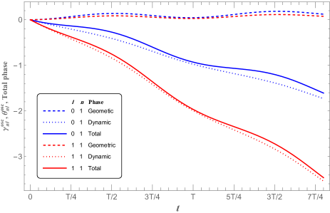
Figure 1: The dynamical, geometrical and total phases.

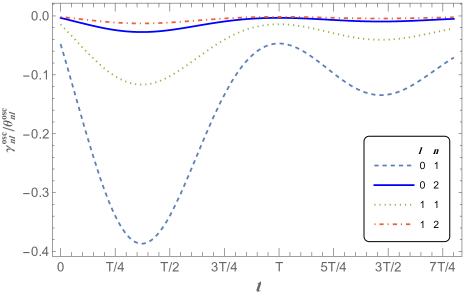
Figure 2: The ratio of geometric and dynamic phases.

IV Acousto-optic example

Consider a metal sphere that fluctuates sinusoidally under an elastic acoustic wave. Such waves can be easily created with frequencies much more than MHz, so that for a well radius about 500 nm, the condition of Eq.(26) is satisfied. For the approximation of the infinite potential well to be acceptable, the metal must have a high work function. This structure can be considered as an example of a soluble system. Now, we have

$$H_{0}(t)|\phi_{nlm}^{\rm{osc}}\rangle=i\hbar\frac{\partial}{\partial t}|\phi_{nlm}^{\rm{osc}}\rangle.$$ (33)

Here,

$$|\phi_{nlm}^{\rm{osc}}\rangle=|\phi^{0}_{nlm}\rangle e^{-i\eta_{nl}},$$ (34)

where $\eta_{nl}$ is the total phase (dynamical plus geometrical, see Eq. (32))

$$\eta_{nl} = -\frac{\bar{E}_{nl}}{\hbar}t-\frac{\varepsilon_{nl}}{\hbar}t+\zeta_{nl}+\zeta^{\prime}_{nl}$$ (35)

and $|\phi^{0}_{nlm}\rangle$ is the rest of wave function. We can generally write Eq. (35) in the form

$$\eta_{nl}=-\frac{\tilde{E}_{nl}}{\hbar}t+\tilde{\zeta}_{nl},$$ (36)

where, $\tilde{E}_{nl}=\bar{E}_{nl}+\varepsilon_{nl}$ that we call modified time-averaged energy in one period and $\tilde{\zeta}_{nl}=\zeta_{nl}+\zeta^{\prime}_{nl}$ is some periodic function. Now, if we expose this system to electromagnetic fields, we can consider the Hamiltonian of the system as $H(t)=H_{0}+\lambda V(t)$. Considering

$$|\psi\rangle=\sum_{nlm}c_{nlm}(t)|\phi_{nlm}^{\rm{osc}}\rangle$$ (37)

we can solve the Schrödinger equation to have

$$i\hbar\frac{\partial}{\partial t}c_{nlm}(t)=\sum_{n^{\prime}m^{\prime}l^{\prime}}c_{n^{\prime}l^{\prime}m^{\prime}}(t)\langle\phi_{nlm}^{\rm{osc}}|\lambda V(t)|\phi_{n^{\prime}l^{\prime}m^{\prime}}^{\rm{osc}}\rangle.$$ (38)

Note that, one can easily show, that for a typical metal the penetration depth of the electric field is much more than the dimensions of the metal sphere. On the other hand, since $\lambda V=-e\bf E\cdot r$, we simply take the field in the $z$ direction, so that $\lambda V=-eEr\cos\theta$. Therefore,

$$\langle\phi_{nlm}|\lambda V|\phi_{n^{\prime}l^{\prime}m^{\prime}}\rangle=\frac{a_{0}+b\sin\omega t}{a_{0}}\langle\phi_{nlm}^{0}|\lambda V(t)|\phi_{n^{\prime}l^{\prime}m^{\prime}}^{0}\rangle,$$ (39)

where $|\phi_{n^{\prime}l^{\prime}m^{\prime}}^{0}\rangle$ is time independent for constant sphere ($b=0$). Consequently we get

$$i\hbar\frac{\partial}{\partial t}c_{nlm}(t)=\sum_{n^{\prime}m^{\prime}l^{\prime}}c_{n^{\prime}l^{\prime}m^{\prime}}(t)\frac{a_{0}+b\sin\omega t}{a_{0}}e^{-i(\eta_{n^{\prime}l^{\prime}}-\eta_{nl})}$$

$$\hskip 85.35826pt\times\langle\phi_{nlm}^{0}|\lambda V(t)|\phi_{n^{\prime}l^{\prime}m^{\prime}}^{0}\rangle.$$ (40)

Now, if at initial point, the electron is in $n_{0}l_{0}m_{0}$ level, then $c_{nlm}(0)=\delta_{nn_{0}}\delta_{ll_{0}}\delta_{mm_{0}}$ and up to ${\cal O}(\lambda)$ we have

$$i\hbar\frac{\partial}{\partial t}c_{nlm}(t)=\frac{a_{0}+b\sin\omega t}{a_{0}}e^{-i(\eta_{n_{0}l_{0}}-\eta_{nl})}$$

$$\hskip 85.35826pt\times\langle\phi_{nlm}^{0}|\lambda V(t)|\phi_{n_{0}l_{0}m_{0}}^{0}\rangle.$$ (41)

and accordingly,

$$c_{nlm}(t)=\frac{1}{i\hbar}\int_{0}^{t}\frac{a_{0}+b\sin\omega t^{\prime}}{a_{0}}e^{-i\Delta\eta_{nl}}$$

$$\hskip 71.13188pt\times\langle\phi_{nlm}^{0}|\lambda V(t^{\prime})|\phi_{n_{0}l_{0}m_{0}}^{0}\rangle dt^{\prime},$$ (42)

where $\Delta\eta_{nl}=\eta_{n_{0}l_{0}}-\eta_{nl}$. Since the electric field is periodic and Hermitian operator, we can write $V(t)=V_{0}e^{-i\omega_{\rm{ph}}t}+V_{0}^{\dagger}e^{i\omega_{\rm{ph}}t}$, where $\omega_{\rm{ph}}$ is the frequency of photon. On the other hand, since $\tilde{\zeta}_{nl}(t)$ is a periodic function with angular frequency $\omega$, we can write the oscillating terms in Fourier series form as follows:

$$\frac{a_{0}+b\sin\omega t}{a_{0}}e^{-i\tilde{\zeta_{nl}}(t)}=\sum_{k=-\infty}^{\infty}f^{k}_{nl}e^{-ik\omega t}.$$ (43)

Therefore,

$$c_{nlm}(t) = \frac{1}{i\hbar}\sum_{k}f^{k}_{nl}\bigg{[}\langle\phi_{nlm}^{0}|\lambda V_{0}|\phi_{n_{0}l_{0}m_{0}}^{0}\rangle\int_{0}^{t}e^{-i(\Delta\tilde{E}_{nl}+\hbar\omega_{\rm{ph}}+\hbar k\omega)t/\hbar}dt^{\prime}$$ (44)

$$\hskip 45.52458pt+\langle\phi_{nlm}^{0}|\lambda V_{0}^{\dagger}|\phi_{n_{0}l_{0}m_{0}}^{0}\rangle\int_{0}^{t}e^{-i(\Delta\tilde{E}_{nl}-\hbar\omega_{\rm{ph}}+\hbar k\omega)t/\hbar}dt^{\prime}\bigg{]}$$

$$= \frac{1}{i\hbar}\sum_{k}f^{k}_{nl}\bigg{\{}\langle\phi_{nlm}^{0}|\lambda V_{0}|\phi_{n_{0}l_{0}m_{0}}^{0}\rangle e^{-i(\Delta\tilde{E}_{nl}+\hbar\omega_{\rm{ph}}+\hbar k\omega)t/2\hbar}\mbox{sinc}\left[(\Delta\tilde{E}_{nl}+\hbar\omega_{\rm{ph}}+\hbar k\omega)t/2\hbar\right]t$$

$$\hskip 14.22636pt+\langle\phi_{nlm}^{0}|\lambda V^{\dagger}_{0}|\phi_{n_{0}l_{0}m_{0}}^{0}\rangle e^{-i(\Delta\tilde{E}_{nl}-\hbar\omega_{\rm{ph}}+\hbar k\omega)t/2\hbar}\mbox{sinc}\left[(\Delta\tilde{E}_{nl}-\hbar\omega_{\rm{ph}}+\hbar k\omega)t/2\hbar\right]t\bigg{\}}.$$

To have the probability, we should multiply Eq. (44) in its complex conjugate. At large $t$ we have

$$\left[t\ \mbox{sinc}(tx/2)\right]^{2}=\frac{\sin^{2}(tx/2)}{(x/2)^{2}}\cong 2\pi\delta(x)t.$$

For the transition rate we have

$$\Gamma_{n_{0}l_{0}m_{0}\to nlm} = \frac{2\pi}{\hbar^{2}}\sum_{k}|f^{k}_{nl}|^{2}\Bigg{\{}|\langle\phi_{nlm}^{0}|\lambda V_{0}|\phi_{n_{0}l_{0}m_{0}}^{0}\rangle|^{2}\delta\left[\frac{\Delta\tilde{E}_{nl}}{\hbar}+\omega_{ph}+k\omega\right]$$ (45)

$$\hskip 56.9055pt+|\langle\phi_{nlm}^{0}|\lambda V_{0}^{\dagger}|\phi_{n_{0}l_{0}m_{0}}^{0}\rangle|^{2}\delta\left[\frac{\Delta\tilde{E}_{nl}}{\hbar}-\omega_{ph}+k\omega\right]\Bigg{\}}.$$

This is just the transition rate for dielectric radiation modified with respect to oscillation. From Eq. (45) we can understand that if the energy gap between the incident photon $\omega_{\rm{ph}}$, and difference of the modified energy of two levels $\Delta\tilde{E}_{nl}$, is equal to the integer multiple of oscillation frequency $\omega$, we will also have absorption or radiation peaks. Here, the effect of geometric phase is hidden in the $\Delta\tilde{E}_{nl}$.

V Summary

The geometric phase for spherical infinite potential well with moving wall in two different cases has been considered. First, when the radius of well increases (or decreases) monotonically. The counterpart of this problem in one dimension is standard and well-known. We have shown that there is a way to observe some manifestations of geometric phase, though the parameter space of this problem is one-dimensional. To solve this problem we have, at first, found the wave functions which satisfy the Schrödinger equation. Second, when the radius changes oscillatory. This problem is closer to physical situations. For this case, we have also solved the Schrödinger equation and found its solutions approximately. For both cases, we compute the geometrical phases. In the other section, we have derived the transition rate for a possible real situation which manifests the effect of geometric phase . We have shown that, in an acousto-optic case, the absorption or radiation peaks will appear if the energy gap between the incident photon and the difference of modified averaged energy of two levels due to Berry phase, is equal to the integer multiple of oscillation frequency.

References

• (1) M V Berry, P. Roy. Soc A-Math. Phy. 392, 45 (1984)
• (2) A Shapere and F Wilczek, Geometric Phases in Physics (World Scientific, Singapore, 1989)
• (3) J A Cina, Chem. Phys. Lett. 132, 393 (1986)
• (4) D Xiao, M C Chang and Q Niu, Rev. Mod. Phys. 82, 1959 (2010)
• (5) M Todorić, B Klajn, D Jukić and H Buljan Phys. Rev. A 102, 013322 (2020)
• (6) A Hannonen, H Partanen, J Tervo, T Setälä and A.T. Friberg Phys. Rev. A 99, 053826 (2019)
• (7) F Ghahari, et al. Science 356, 845 (2017)
• (8) C G Yale, F J Heremans, B B Zhou, A Auer, G Burkard and D D Awschalom, Nat. photonics 10, 184 (2016)
• (9) C Dutreix, H González-Herrero, I Brihuega, M I Katsnelson, C Chapelier and V T Renard,Nature 574, 219 (2019)
• (10) M Baggio, V Niarchos and K Papadodimas. J. high Energy Phys. 04, 1 (2017)
• (11) P S Hsin, A Kapustin and R Thorngren, Phys. Rev. B 102, 245113 (2020).
• (12) S W Doescher and M H Rice, Am. J. Phys. 37, 1246 (1969)
• (13) S V Mousavi, Europhys. Lett. 99, 30002 (2012)