Large Eddy Simulations of Supersonic Jet Flows for Aeroacoustic Applications

Abstract

Abstract

Current design constraints have encouraged the studies of aeroacoustics fields around compressible jet flows. The present work addresses the numerical study of unsteady turbulent jet flows for aeroacoustic analyses of main engine rocket plumes. A novel large eddy simulation (LES) tool is developed in order to reproduce high fidelity results of compressible jet flows which could be used for aeroacoustic studies with the Ffowcs Williams and Hawkings approach. The numerical solver is an upgrade of an existing Reynolds-averaged Navier-Stokes solver previously developed in the group. The original framework is rewritten in a modern fashion and intensive parallel computation capabilities have been added to the code. The LES formulation is written using the finite difference approach. The energy equation is carefully discretized in order to model the energy equation of the filtered Navier-Stokes formulation. The classical Smagorinsky model is the chosen subgrid scale closure for the present work. Numerical simulations of perfectly expanded jets are performed and compared with the literature in order to validate the new solver. Moreover, speedup and the computational performance of the code are evaluated and discussed. Flow results are used for an initial evaluation of the noise radiated from the rocket plume.

Nomenclature

Abbreviations

1-D: One dimensional
2-D: Two dimensional
3-D: Three dimensional
CFD: Computational fluid dynamics
CFL: Courant-Friedrichs-Lewys number
CGNS: CFD general notation system
EDQNM: Eddy-damped quasi-normal Markovian
IAE: Instituto de Aeronáutica e Espaço
LES: Large eddy simulation
MPI: Message passing interface
SGS: Subgrid scale

English Characters

$a$: Speed of sound
$B_{i}$: Subgrid terms of energy equation
$C_{p}$: Specific heat at constant pressure
$C_{s}$: Smagorinsky constant
$C_{v}$: Specific heat at constant volume
$d$: Inlet diameter
$\mathbf{d}$: Artificial dissipation term
$\mathcal{D}$: SGS viscous diffusion term
$E$: Total energy per mass unity
$\mathbf{E}_{e}$: Inviscid flux vector in the axial direction
$\mathbf{E}_{v}$: Viscous flux vector in the axial direction
$\mathbf{F}_{e}$: Inviscid flux vector in the radial direction
$\mathbf{F}_{v}$: Viscous flux vector in the radial direction
$\mathbf{G}_{e}$: Inviscid flux vector in the azimuthal direction
$\mathbf{G}_{v}$: Viscous flux vector in the azimuthal direction
$J$: Jacobian of the coordinate transformation
$l$: Reference lenght
$M$: Mach number
$p$: Static pressure
$Pr$: Prandtl number
$q$: Heat flux vector
$\mathcal{Q}_{j}$: Components of SGS temperature flux
$R$: Gas constant
$\mathbf{R}$: Riemman invariant
$Re$: Reynolds number
$RHS$: Right hand side of the equation
$S_{1}$: Sutherland constant
$S_{ij}$: Components of rate-of-strain tensor
$Sp_{N}$: Speedup for N processors
$t$: time
$T$: Temperature
$T_{N}$: CPU time using N processors
$T_{s}$: CPU time using single processor
u: Velocity vector
$u$: Components of the velocity vector in a Catesian coordinate system
$U$: Component of the contravariant velocity in the axial direction
$V$: Component of the contravariant velocity in the radial direction
$\vec{n}$ : Unity outward normal vector
$W$: Component of the contravariant velocity in the azimuthal direction
$\mathcal{W}$: Modified conservative properties of Turkel and Vatsa artificial dissipation
x: Spacial coordinates of a Cartesian coordinate system

Greek Characters

$\alpha_{l}$: Runge-Kutta constants
$\beta_{j}$: Viscous terms of energy equation
$\gamma$: Specific heat ratio
$\Delta t$: Time-step
$\mathcal{E}$: SGS viscous dissipation
$\epsilon$: Turkel and Vatsa artificial dissipation terms
$\zeta$: Azimuthal direction
$\eta$: Radial direction
$\kappa$: Thermal conductivity
$\lambda$: Spectral radius-based scaling factor
$\lambda_{\zeta}$: Spectral radii in the $\zeta$ direction
$\lambda_{\eta}$: Spectral radii in the $\eta$ direction
$\lambda_{\xi}$: Spectral radii in the $\xi$ direction
$\mu$: Dynamic viscosity
$\nu$: Kinematicc viscosity
$\xi$: Axial direction
$\Pi_{dil}$: SGS pressure-diatation
$\rho$: Density
$\sigma_{ij}$: Components of the SGS tensor
$\tau_{ij}:$ Shear-stress tensor

Subscripts

$j$: Relative to the jet
$\infty$: Relative to the freestream
$e$: Relative to interior domain
$f$: Relative to boundary face
$sgs$: subgrid property

1 Introduction

One of the main design issues related to launch vehicles lies on noise emission originated from the complex interaction between the high-temperature/high-velocity exhaustion gases and the atmospheric air. These emissions yield very high noise levels, which must be minimized due to several design constraints. For instance, the resulting pressure fluctuations can damage the solid structure of different parts of the launcher by vibrational acoustic stress. Therefore, it is a design constraint to consider the loads resulting from acoustic sources in the structural dimensioning of large launch vehicles during the take off and also during the transonic flight. Moreover, one cannot neglect the energy dissipation effect caused by the acoustic waves generated even if the vehicles is far from the ground. Theoretically, all chemical energy should be converted into kinectic energy. However, in reallity, the noise generation consumes part of the chemical energy.

The acoustic design constraints have encouraged the studies of aeroacoustic fields around compressible jet flows. Instituto de Aeronautica e Espaço (IAE) in Brazil is interested in this flow configuration for rocket design applications. Unsteady property fields of the flow are necessary for the aerocoustic studies. Therefore, the present work addresses the development of a new numerical tool for the study of unsteady turbulent compressible jet flows for aeroacoustic applications. The novel code uses the large eddy simulation (LES) formulation due to recent successful results of such approach for similar flow configurations [1, 2]. Such formulation is able to reproduce high fidelity results for compressible jet flows, which, in turn, could be used for aeroacoustic studies using the Ffowcs Williams and Hawkings approach [3].

The solver is an upgrade of a finite difference Reynolds-averaged Navier-Stokes (RANS) solver developed to study turbulent flows for aerospace applications [4]. Generally, LES calculations demand very dense grids. Hence, high performance computing (HPC) is a requirement for such simulations. Dynamic memory allocation and parallel computation capabilities have been added to the legacy code [4]. The communication between processors is performed by message passing interface (MPI) protocols. The CFD general notation system (CGNS) is also included in the numerical tool. The LES formulation is written using the finite difference approach. Inviscid numerical fluxes are calculated using a second-order accurate centered scheme with the explicit addition of artificial dissipation. A five-step second-order accurate Runge-Kutta scheme is the chosen time marching method.

The System I formulation [5] is used here in order to model the filtered terms of the energy equation. The Smagorinsky [6] model is the chosen model to calculate the components of the subgrid scale (SGS) tensor. The Eidson [7] hypothesis is the chosen model to calculate the subgrid scale terms of the filtered energy equation. For the sake of simplicity, only perfectly expanded jet configurations are studied in the current work. The LES tool is validated through a comparison of results of perfectly expanded jets with numerical [1, 8] and experimental [9, 10] data. Moreover, the computational performance of the solver is evaluated and discussed. Flow results are used for an initial evaluation of the noise radiated from the rocket plume.

2 Large Eddy Simulation Formulation

The numerical strategy used in the present study is based on the System I filtered compressible Navier-Stokes equations [5] formulated as

$$\displaystyle\frac{\partial\overline{\rho}}{\partial t}+\frac{\partial}{\partial x_{j}}\left(\overline{\rho}\widetilde{u_{j}}\right) = 0\,\mbox{,}$$ (1)

$$\displaystyle\frac{\partial}{\partial t}\left(\overline{\rho}\widetilde{u_{i}}\right)+\frac{\partial}{\partial x_{j}}\left(\overline{\rho}\widetilde{u_{i}}\widetilde{u_{j}}\right)+\frac{\partial\overline{p}}{\partial x_{i}}-\frac{\partial\check{\tau}_{ij}}{\partial x_{j}} = -\frac{\partial}{\partial x_{j}}\left[\sigma_{ij}-\left(\overline{\tau_{ij}}-\check{\tau}_{ij}\right)\right]\,\mbox{,}$$ (2)

$$\displaystyle\frac{\partial\overline{\rho}\check{E}}{\partial t}+\frac{\partial\left(\overline{\rho}\check{E}+\overline{p}\right)\widetilde{u_{j}}}{\partial x_{j}}-\frac{\partial\check{\tau}_{ij}\widetilde{u_{i}}}{\partial x_{j}}+\frac{\partial\check{q}_{j}}{\partial x_{j}} = -B_{1}-B_{2}-B_{3}+B_{4}+B_{5}+B_{6}-B_{7}\,\mbox{,}$$ (3)

in which $t$ and $x_{i}$ are independent variables representing time and spatial coordinates of a Cartesian coordinate system x, respectively. The components of the velocity vector u are written as $u_{i}$, and $i=1,2,3$. Density, pressure and total energy per mass unit are denoted by $\rho$, $p$ and $E$, respectively. $\overline{\left(\cdot\right)}$ stands for filtered properties and $\tilde{\left(\cdot\right)}$ stands for Favre averaged properties. The filtered heat flux, $\check{q}_{j}$, is given by

$$\check{q}_{j}=\left[\kappa(\tilde{T})\right]\frac{\partial\tilde{T}}{\partial x_{j}}\,\mbox{,}$$ (4)

where $\tilde{T}$ is the averaged static temperature and $\kappa$ is the thermal conductivity, which can by expressed by

$$\kappa(T)=\left[\mu(T)\right]\frac{C_{p}}{Pr}\,\mbox{.}$$ (5)

The thermal conductivity is a function of the specific heat at constant pressure, $Cp$, of the Prandtl number, $Pr$, which is equal to $0.72$ for air, and of the dynamic viscosity, $\mu$. The last is calculated using the Sutherland Law,

$$\mu(T)=\mu_{\infty}\left(\frac{T}{T_{\infty}}\right)^{\frac{3}{2}}\frac{T_{0}+S_{1}}{T+S_{1}} \mbox{with}\>S_{1}=110.4K\,\mbox{.}$$ (6)

In the present work, $\check{\tau}_{ij}$ is calculated using the Stokes hypothesis for Newtonian fluids,

$$\check{\tau}_{ij}=2\left[\mu(\tilde{T})\right]\left(\check{S}_{ij}-\frac{1}{3}\delta_{ij}\check{S}_{kk}\right)\,\mbox{,}$$ (7)

in which $\check{S}_{ij}$, components of rate-of-strain tensor, is given by

$$\check{S}_{ij}=\frac{1}{2}\left(\frac{\partial\widetilde{u_{i}}}{\partial x_{j}}+\frac{\partial\widetilde{u_{j}}}{\partial x_{i}}\right)\,\mbox{.}$$ (8)

In order to close the system of equations the density, the static pressure and the static temperature are correlated by the equation of state given by

$$\overline{p}=\overline{\rho}R\tilde{T}\,\mbox{,}$$ (9)

where $R$ is the gas constant, written as

$$R=C_{p}-C_{v}\,\mbox{,}$$ (10)

and $C_{v}$ is the specif heat at constant volume. The System I formulation [5] neglects the double correlation term of the total energy per mass unity and writes

$$\overline{\rho E}=\overline{\rho}\check{E}=\frac{\overline{p}}{\gamma-1}+\frac{1}{2}\rho\tilde{u}_{i}\tilde{u}_{i}\,\mbox{,}$$ (11)

in which $\gamma$ is the specif heat ratio written as $\gamma=Cp/Cv$. The components of the SGS stress tensor, $\sigma$, are given by

$$\sigma_{ij}=\overline{\rho}\left(\widetilde{u_{i}u_{j}}-\widetilde{u_{i}}\widetilde{u_{j}}\right)\,\mbox{,}$$ (12)

and the SGS $B_{i}$ terms are written as

$$B_{1}=\frac{1}{(\gamma-1)}\frac{\partial}{\partial x_{j}}\left(\overline{pu_{j}}-\overline{p}\widetilde{u_{j}}\right)=\frac{\partial C_{v}\mathcal{Q}_{j}}{\partial x_{j}}\,\mbox{,}$$ (13)

$$B_{2}=\overline{p\frac{\partial u_{k}}{\partial x_{k}}}-\overline{p}\frac{\partial\widetilde{u_{k}}}{\partial x_{k}}=\Pi_{dil}\,\mbox{,}$$ (14)

$$B_{3}=\frac{\partial}{\partial x_{j}}\left(\sigma_{kj}\widetilde{u_{k}}\right)\,\mbox{,}$$ (15)

$$B_{4}=\sigma_{kj}\frac{\partial}{\partial x_{j}}\widetilde{u_{k}}\,\mbox{,}$$ (16)

$$B_{5}=\overline{\tau_{kj}\frac{\partial}{\partial x_{j}}u_{k}}-\overline{\tau_{ij}}\frac{\partial}{\partial x_{j}}\widetilde{u_{k}}=\mathcal{E}\,\mbox{,}$$ (17)

$$B_{6}=\frac{\partial}{\partial x_{j}}\left(\overline{\tau_{ij}}\widetilde{u_{i}}-\check{\tau}_{ij}\widetilde{u_{i}}\right)=\frac{\partial\mathcal{D}}{\partial x_{j}}\,\mbox{,}$$ (18)

$$B_{7}=\frac{\partial}{\partial x_{j}}\left(\overline{q_{j}}-\check{q}_{j}\right)\,\mbox{,}$$ (19)

where $\mathcal{Q}_{j}$ is the SGS temperature flux, written as

$$\mathcal{Q}_{j}=\overline{\rho}\left(\widetilde{u_{j}T}-\widetilde{u_{j}}\widetilde{T}\right)\,\mbox{,}$$ (20)

$\Pi_{dil}$ is the SGS pressure-dilatation term, $\mathcal{E}$ is the SGS viscous dissipation and $\mathcal{D}$ is the SGS viscous diffusion term.

3 Subgrid Scale Modeling

The SGS terms presented in Eqs. (2) and (3) cannot be directly calculated. Subgrid scale models are necessary in order to close the LES set of equations. The closure models presented here are based on homogeneous turbulence theory, which is usually developed in spectral space as an atempt to quantify the interaction between the different scales of turbulence.

3.1 Subgrid Scale Viscosity

The SGS stress tensor is here calculated using the concept that the forward energy cascade is analogous to the molecular mechanisms represented by the molecular viscosity whose mathematical structure follows the Boussinesq hypothesis [11] to explicitly introduce the subgrid scale viscosity, $\mu_{sgs}$,

$$\sigma_{ij}^{d}=\sigma_{ij}-\frac{1}{3}\delta_{ij}\sigma_{kk}=-2\mu_{sgs}\left(\check{S}_{ij}-\frac{1}{3}\check{S}_{kk}\right)\,\mbox{.}$$ (21)

The isotropic portion of the SGS stress tensor is generally weak with respect to the thermodynamic pressure [12]. Therefore, $\sigma_{kk}$ is neglected in the present paper and $\sigma_{ij}$ is written as

$$\sigma_{ij}=-2\mu_{sgs}\left(\check{S}_{ij}-\frac{1}{3}\check{S}_{kk}\right)\,\mbox{.}$$ (22)

The Smagorinsky model [6, 13] is used to calculate the SGS viscosity and it is given by

$$\mu_{sgs}=\overline{\rho}\left(C_{s}\Delta\right)^{2}\left(2\check{S}_{ij}\check{S}_{ij}\right)^{\frac{1}{2}}\,\mbox{,}$$ (23)

and $C_{s}$ is the Smagorinsky constant. Several attempts can be found in the literature regarding the evaluation of the Smagorinsky constant. The value of this constant is adjusted to improve the results of different flow configurations. In pratical terms, the Smagorinsky constant assumes value ranging from 0.1 to 0.2 depending on the flow. The present work uses $C_{s}=0.18$ as suggested by Lilly [14].

3.2 Subgrid Scale Modeling of the Energy Equation

Some of the SGS terms within the System I formulation [5] are not directly computable. Therefore, modeling is applied in order to close the system. Several papers in the literature [2, 12, 15, 16, 17, 18] evaluate the relevance of the SGS terms on different applications. The LES community commonly uses the hypothesis of Eidson [7], which assumes that the energy transfer from the resolved scales is proportional to the gradient of the resolved temperature [2]. The proportionality coefficient is the subgrid scale conductivity, $\kappa_{sgs}$, which is linked to the subgrid scale viscosity through the relation

$$\kappa_{sgs}=\frac{\overline{\rho}\,\nu_{sgs}\,C_{p}}{{Pr}_{sgs}}\,\mbox{,}$$ (24)

in which $Pr_{sgs}$ is the SGS Prandtl number. The eddy-damped quasi-normal Markovian (EDQNM) theory [19] considers $Pr_{sgs}=0.6$. In the present work, the concept of SGS conductivity, $\kappa_{sgs}$, is used in order to model $B_{1}+B_{2}$, i.e.,

$$B_{1}+B_{2}=-\frac{\partial}{\partial x_{j}}\left(\kappa_{sgs}\frac{\partial\tilde{T}}{\partial x_{j}}\right)\,\mbox{,}$$ (25)

Following the work of Larcheveque [20], $B_{4}$, $B_{5}$, $B_{6}$ and $B_{7}$ are neglected in the present paper.

3.3 Shear-Stress Tensor Modeling

The difference between the shear-stress tensors at the right-hand side of the momentum equations is neglected in the present work,

$$\overline{\tau_{ij}}-\check{\tau}_{ij}=0$$ (26)

4 Transformation of Coordinates

The legacy code formulation [4] was originally written in the a general curvilinear coordinate system in order to facilitate the implementation and add more generality for the CFD tool. This approach is kept in the present LES solver for the simulation of compressible jet flows. Hence, the filtered Navier-Stokes equations can be written in strong conservation form for a 3-D general curvilinear coordinate system as

$$\frac{\partial\hat{Q}}{\partial\mathcal{T}}+\frac{\partial}{\partial\xi}\left(\hat{\mathbf{E}_{e}}-\hat{\mathbf{E}_{v}}\right)+\frac{\partial}{\partial\eta}\left(\hat{\mathbf{F}_{e}}-\hat{\mathbf{F}_{v}}\right)+\frac{\partial}{\partial\zeta}\left(\hat{\mathbf{G}_{e}}-\hat{\mathbf{G}_{v}}\right)=0\,\mbox{.}$$ (27)

In the present work, the chosen general coordinate transformation is given by

$$\mathcal{T} = t\,\mbox{,}$$

$$\xi = \xi\left(x,y,z,t\right)\,\mbox{,}$$

$$\eta = \eta\left(x,y,z,t\right)\,\mbox{,}$$ (28)

$$\zeta = \zeta\left(x,y,z,t\right)\ \,\mbox{.}$$

In the jet flow configuration, $\xi$ is the axial jet flow direction, $\eta$ is the radial direction and $\zeta$ is the azimuthal direction. The vector of conserved properties is written as

$$\hat{Q}=J^{-1}\left[\overline{\rho}\quad\overline{\rho}\tilde{u}\quad\overline{\rho}\tilde{v}\quad\overline{\rho}\tilde{w}\quad\overline{e}\right]^{T}\quad\mbox{,}$$ (29)

where the Jacobian of the transformation, $J$, is given by

$$J=\left(x_{\xi}y_{\eta}z_{\zeta}+x_{\eta}y_{\zeta}z_{\xi}+x_{\zeta}y_{\xi}z_{\eta}-x_{\xi}y_{\zeta}z_{\eta}-x_{\eta}y_{\xi}z_{\zeta}-x_{\zeta}y_{\eta}z_{\xi}\right)^{-1}\,\mbox{,}$$ (30)

and

$$\displaystyle x_{\xi}=\frac{\partial x}{\partial\xi}\,\mbox{,} \displaystyle x_{\eta}=\frac{\partial x}{\partial\eta}\,\mbox{,} \displaystyle x_{\zeta}=\frac{\partial x}{\partial\zeta}\,\mbox{,}$$

$$\displaystyle y_{\xi}=\frac{\partial y}{\partial\xi}\,\mbox{,} \displaystyle y_{\eta}=\frac{\partial y}{\partial\eta}\,\mbox{,} \displaystyle y_{\zeta}=\frac{\partial y}{\partial\zeta}\,\mbox{,}$$ (31)

$$\displaystyle z_{\xi}=\frac{\partial z}{\partial\xi}\,\mbox{,} \displaystyle z_{\eta}=\frac{\partial z}{\partial\eta}\,\mbox{,} \displaystyle z_{\zeta}=\frac{\partial z}{\partial\zeta}\,\mbox{.}$$

The inviscid flux vectors, $\hat{\mathbf{E}}_{e}$, $\hat{\mathbf{F}}_{e}$ and $\hat{\mathbf{G}}_{e}$, are given by

$$\hat{\mathbf{E}}_{e}=J^{-1}\left\{\begin{array}[]{c}\overline{\rho}U\\ \overline{\rho}\tilde{u}U+\overline{p}\xi_{x}\\ \overline{\rho}\tilde{v}U+\overline{p}\xi_{y}\\ \overline{\rho}\tilde{w}U+\overline{p}\xi_{z}\\ \left(\overline{e}+\overline{p}\right)U-\overline{p}\xi_{t}\end{array}\right\}\,\mbox{,} \hat{\mathbf{F}}_{e}=J^{-1}\left\{\begin{array}[]{c}\overline{\rho}V\\ \overline{\rho}\tilde{u}V+\overline{p}\eta_{x}\\ \overline{\rho}\tilde{v}V+\overline{p}\eta_{y}\\ \overline{\rho}\tilde{w}V+\overline{p}\eta_{z}\\ \left(\overline{e}+\overline{p}\right)V-\overline{p}\eta_{t}\end{array}\right\}\,\mbox{,} \hat{\mathbf{G}}_{e}=J^{-1}\left\{\begin{array}[]{c}\overline{\rho}W\\ \overline{\rho}\tilde{u}W+\overline{p}\zeta_{x}\\ \overline{\rho}\tilde{v}W+\overline{p}\zeta_{y}\\ \overline{\rho}\tilde{w}W+\overline{p}\zeta_{z}\\ \left(\overline{e}+\overline{p}\right)W-\overline{p}\zeta_{t}\end{array}\right\}\,\mbox{.}$$ (47)

The contravariant velocity components, $U$, $V$ and $W$, are calculated as

$$U=\xi_{t}+\xi_{x}\overline{u}+\xi_{y}\overline{v}+\xi_{z}\overline{w}\,\mbox{,}$$

$$V=\eta_{t}+\eta_{x}\overline{u}+\eta_{y}\overline{v}+\eta_{z}\overline{w}\,\mbox{,}$$ (48)

$$W=\zeta_{t}+\zeta_{x}\overline{u}+\zeta_{y}\overline{v}+\zeta_{z}\overline{w}\,\mbox{.}$$

The metric terms are given by

$$\xi_{x}=J\left(y_{\eta}z_{\zeta}-y_{\zeta}z_{\eta}\right)\,\mbox{,} \xi_{y}=J\left(z_{\eta}x_{\zeta}-z_{\zeta}x_{\eta}\right)\,\mbox{,} \xi_{z}=J\left(x_{\eta}y_{\zeta}-x_{\zeta}y_{\eta}\right)\,\mbox{,}$$

$$\eta_{x}=J\left(y_{\eta}z_{\xi}-y_{\xi}z_{\eta}\right)\,\mbox{,} \eta_{y}=J\left(z_{\eta}x_{\xi}-z_{\xi}x_{\eta}\right)\,\mbox{,} \eta_{z}=J\left(x_{\eta}y_{\xi}-x_{\xi}y_{\eta}\right)\,\mbox{,}$$ (49)

$$\zeta_{x}=J\left(y_{\xi}z_{\eta}-y_{\eta}z_{\xi}\right)\,\mbox{,} \zeta_{y}=J\left(z_{\xi}x_{\eta}-z_{\eta}x_{\xi}\right)\,\mbox{,} \zeta_{z}=J\left(x_{\xi}y_{\eta}-x_{\eta}y_{\xi}\right)\,\mbox{,}$$

$$\xi_{t}=-x_{\mathcal{T}}\xi_{x}-y_{\mathcal{T}}\xi_{y}-z_{\mathcal{T}}\xi_{z}\,\mbox{,} \eta_{t}=-x_{\mathcal{T}}\eta_{x}-y_{\mathcal{T}}\eta_{y}-z_{\mathcal{T}}\eta_{z}\,\mbox{,} \zeta_{t}=-x_{\mathcal{T}}\zeta_{x}-y_{\mathcal{T}}\zeta_{y}-z_{\mathcal{T}}\zeta_{z}\,\mbox{.}$$

The viscous flux vectors, $\hat{\mathbf{E}}_{v}$, $\hat{\mathbf{F}}_{v}$ and $\hat{\mathbf{G}}_{v}$, are written as

$$\hat{\mathbf{E}}_{v}=J^{-1}\left\{\begin{array}[]{c}0\\ \xi_{x}\hat{\tau}_{xx}+\xi_{y}\hat{\tau}_{xy}+\xi_{z}\hat{\tau}_{xz}\\ \xi_{x}\hat{\tau}_{xy}+\xi_{y}\hat{\tau}_{yy}+\xi_{z}\hat{\tau}_{yz}\\ \xi_{x}\hat{\tau}_{xz}+\xi_{y}\hat{\tau}_{yz}+\xi_{z}\hat{\tau}_{zz}\\ \xi_{x}{\beta}_{x}+\xi_{y}{\beta}_{y}+\xi_{z}{\beta}_{z}\end{array}\right\}\,\mbox{,}$$ (50)

$$\hat{\mathbf{F}}_{v}=J^{-1}\left\{\begin{array}[]{c}0\\ \eta_{x}\hat{\tau}_{xx}+\eta_{y}\hat{\tau}_{xy}+\eta_{z}\hat{\tau}_{xz}\\ \eta_{x}\hat{\tau}_{xy}+\eta_{y}\hat{\tau}_{yy}+\eta_{z}\hat{\tau}_{yz}\\ \eta_{x}\hat{\tau}_{xz}+\eta_{y}\hat{\tau}_{yz}+\eta_{z}\hat{\tau}_{zz}\\ \eta_{x}{\beta}_{x}+\eta_{y}{\beta}_{y}+\eta_{z}{\beta}_{z}\end{array}\right\}\,\mbox{,}$$ (51)

$$\hat{\mathbf{G}}_{v}=J^{-1}\left\{\begin{array}[]{c}0\\ \zeta_{x}\hat{\tau}_{xx}+\zeta_{y}\hat{\tau}_{xy}+\zeta_{z}\hat{\tau}_{xz}\\ \zeta_{x}\hat{\tau}_{xy}+\zeta_{y}\hat{\tau}_{yy}+\zeta_{z}\hat{\tau}_{yz}\\ \zeta_{x}\hat{\tau}_{xz}+\zeta_{y}\hat{\tau}_{yz}+\zeta_{z}\hat{\tau}_{zz}\\ \zeta_{x}{\beta}_{x}+\zeta_{y}{\beta}_{y}+\zeta_{z}{\beta}_{z}\end{array}\right\}\,\mbox{,}$$ (52)

where $\beta_{x}$, $\beta_{y}$ and $\beta_{z}$ are defined as

$$\beta_{x}=\hat{\tau}_{xx}\tilde{u}+\hat{\tau}_{xy}\tilde{v}+\hat{\tau}_{xz}\tilde{w}-\overline{q}_{x}\,\mbox{,}$$

$$\beta_{y}=\hat{\tau}_{xy}\tilde{u}+\hat{\tau}_{yy}\tilde{v}+\hat{\tau}_{yz}\tilde{w}-\overline{q}_{y}\,\mbox{,}$$ (53)

$$\beta_{z}=\hat{\tau}_{xz}\tilde{u}+\hat{\tau}_{yz}\tilde{v}+\hat{\tau}_{zz}\tilde{w}-\overline{q}_{z}\mbox{.}$$

and $\hat{\tau}_{ij}$ is given by

$$\hat{\tau}_{ij}=2\left(\mu+\mu_{sgs}\right)\left(\check{S}_{ij}-\frac{1}{3}\check{S}_{kk}\right)\,\mbox{.}$$ (54)

5 Dimensionless Formulation

A convenient nondimensionalization is necessary in to order to achieve a consistent implementation of the governing equations of motion. Dimensionless formulation yields to a more general numerical tool. There is no need to change the formulation for each configuration intended to be simulated. Moreover, dimensionless formulation scales all the necessary properties to the same order of magnitude which is a computational advantage [4]. Dimensionless variables are presented in the present section in order perform the nondimensionalization of Eq. (27)

The dimensionless time, $\underline{\mathcal{T}}$, is written as function of the speed of sound of the jet at the inlet, $a_{j}$, and of a reference lenght, $l$,

$$\underline{\mathcal{T}}=\mathcal{T}\frac{a_{j}}{l}\,\mbox{.}$$ (55)

In the present work $l$ represents the jet entrance diameter $d$. This reference lenght is also applied to write the dimensionless length,

$$\underline{l}=\frac{l}{d}\,\mbox{.}$$ (56)

The dimensionless velocity components are obtained using the speed of sound of the jet at the inlet,

$$\underline{\textbf{u}}=\frac{\textbf{u}}{a_{j}}\,\mbox{.}$$ (57)

Dimensionless pressure and energy are calculated using density and speed of the sound of the jet at the inlet as

$$\underline{p}=\frac{p}{\rho_{j}a_{j}^{2}}\,\mbox{,}$$ (58)

$$\underline{E}=\frac{E}{\rho_{j}a_{j}^{2}}\,\mbox{.}$$ (59)

Dimensionless density, $\underline{\rho}$, temperature, $\underline{T}$ and viscosity, $\underline{\mu}$, are calculated using freestream properties

$$\underline{\rho}=\frac{\rho}{\rho_{j}}\,\mbox{.}$$ (60)

One can use the dimensionless properties described above in order to write the dimensionless form of the RANS equations as

$$\frac{\partial\underline{Q}}{\partial\mathcal{T}}+\frac{\partial\underline{\mathbf{E}}_{e}}{\partial\xi}+\frac{\partial\underline{\mathbf{F}}_{e}}{\partial\eta}+\frac{\partial\underline{\mathbf{G}}_{e}}{\partial\zeta}=\frac{1}{Re}\left(\frac{\partial\underline{\mathbf{E}}_{v}}{\partial\xi}+\frac{\partial\underline{\mathbf{F}}_{v}}{\partial\eta}+\frac{\partial\underline{\mathbf{G}}_{v}}{\partial\zeta}\right)\,\mbox{,}$$ (61)

where the underlined terms are calculated using dimensionless properties and the Reynolds number is based on the jet properties such as the speed of sound, $a_{j}$, density, $\rho_{j}$, viscosity, $\mu_{j}$ and the jet entrance diameter, $d$,

$$Re=\frac{\rho_{j}a_{j}d}{\mu_{j}}\,\mbox{.}$$ (62)

6 Numerical Formulation

The governing equations previously described are discretized in a structured finite difference context for general curvilinear coordinate system [4]. The numerical flux is calculated through a central difference scheme with the explicit addition of the anisotropic scalar artificial dissipation of Turkel and Vatsa [21]. The time integration is performed by an explicit, 2nd-order, 5-stage Runge-Kutta scheme [22, 23]. Conserved properties and artificial dissipation terms are properly treated near boundaries in order to assure the physical correctness of the numerical formulation.

6.1 Spatial Discretization

For the sake of simplicity the formulation discussed in the present section is no longer written using bars. However, the reader should notice that the equations are dimensionless and filtered. The Navier-Stokes equations, presented in Eq. (61), are discretized in space in a finite difference fashion and, then, rewritten as

$$\left(\frac{\partial Q}{\partial\mathcal{T}}\right)_{i,j,k}\ =\ -RHS_{i,j,k}\,\mbox{,}$$ (63)

where $RHS$ is the right hand side of the equation and it is written as function of the numerical flux vectors at the interfaces between grid points,

$${RHS}_{i,j,k} = \frac{1}{\Delta\xi}\left({\mathbf{E}_{e}}_{(i+\frac{1}{2},j,k)}-{\mathbf{E}_{e}}_{(i-\frac{1}{2},j,k)}-{\mathbf{E}_{v}}_{(i+\frac{1}{2},j,k)}+{\mathbf{E}_{v}}_{(i-\frac{1}{2},j,k)}\right)$$

$$\frac{1}{\Delta\eta}\left({\mathbf{F}_{e}}_{(i,j+\frac{1}{2},k)}-{\mathbf{F}_{e}}_{(i,j-\frac{1}{2},k)}-{\mathbf{F}_{v}}_{(i,j+\frac{1}{2},k)}+{\mathbf{F}_{v}}_{(i,j-\frac{1}{2},k)}\right)$$

$$\frac{1}{\Delta\zeta}\left({\mathbf{G}_{e}}_{(i,j,k+\frac{1}{2})}-{\mathbf{G}_{e}}_{(i,j,k-\frac{1}{2})}-{\mathbf{G}_{v}}_{(i,j,k+\frac{1}{2})}+{\mathbf{G}_{v}}_{(i,j,k-\frac{1}{2})}\right)\,\mbox{.}$$

For the general curvilinear coordinate case $\Delta\xi=\Delta\eta=\Delta\zeta=1$. The anisotropic scalar artificial dissipation method of Turkel and Vatsa [21] is implemented through the modification of the inviscid flux vectors, $\mathbf{E}_{e}$, $\mathbf{F}_{e}$ and $\mathbf{G}_{e}$. The numerical scheme is nonlinear and allows the selection between artificial dissipation terms of second and fourth differences, which is very important for capturing discontinuities in the flow. The numerical fluxes are calculated at interfaces in order to reduce the size of the calculation cell and, therefore, facilitate the implementation of second derivatives since the the concept of numerical fluxes vectors is used for flux differencing. Only internal interfaces receive the corresponding artificial dissipation terms, and differences of the viscous flux vectors use two neighboring points of the interface.

The inviscid flux vectors, with the addition of the artificial dissipation contribution, can be written as

$${\mathbf{E}_{e}}_{(i\pm\frac{1}{2},j,k)}=\frac{1}{2}\left({\mathbf{E}_{e}}_{(i,j,k)}+{\mathbf{E}_{e}}_{(i\pm 1,j,k)}\right)-J^{-1}\mathbf{d}_{(i\pm\frac{1}{2},j,k)}\,\mbox{,}$$

$${\mathbf{F}_{e}}_{(i,j\pm\frac{1}{2},k)}=\frac{1}{2}\left({\mathbf{F}_{e}}_{(i,j,k)}+{\mathbf{F}_{e}}_{(i,j\pm 1,k)}\right)-J^{-1}\mathbf{d}_{(i,j\pm\frac{1}{2},k)}\,\mbox{,}$$ (65)

$${\mathbf{G}_{e}}_{(i,j,k\pm\frac{1}{2})}=\frac{1}{2}\left({\mathbf{G}_{e}}_{(i,j,k)}+{\mathbf{G}_{e}}_{(i,j,k\pm 1)}\right)-J^{-1}\mathbf{d}_{(i,j,k\pm\frac{1}{2})}\,\mbox{,}$$

in which the $\mathbf{d}_{(i\pm 1,j,k)}$,$\mathbf{d}_{(i,j\pm 1,k)}$ and $\mathbf{d}_{(i,j,k\pm 1)}$ terms are the Turkel and Vatsa [21] artificial dissipation terms in the $i$, $j$, and $k$ directions respectively. The scaling of the artificial dissipation operator in each coordinate direction is weighted by its own spectral radius of the corresponding flux Jacobian matrix, which gives the non-isotropic characteristics of the method [4]. The artificial dissipation contribution in the $\xi$ direction is given by

$$\mathbf{d}_{(i+\frac{1}{2},j,k)} = \lambda_{(i+\frac{1}{2},j,k)}\left[\epsilon_{(i+\frac{1}{2},j,k)}^{(2)}\left(\mathcal{W}_{(i+1,j,k)}-\mathcal{W}_{(i,j,k)}\right)\right.$$

$$\epsilon_{(i+\frac{1}{2},j,k)}^{(4)}\left(\mathcal{W}_{(i+2,j,k)}-3\mathcal{W}_{(i+1,j,k)}+3\mathcal{W}_{(i,j,k)}-\mathcal{W}_{(i-1,j,k)}\right)\left.\right]\,\mbox{,}$$

in which

$$\epsilon_{(i+\frac{1}{2},j,k)}^{(2)} = k^{(2)}\mbox{max}\left(\nu_{(i+1,j,k)}^{d},\nu_{(i,j,k)}^{d}\right)\,\mbox{,}$$ (67)

$$\epsilon_{(i+\frac{1}{2},j,k)}^{(4)} = \mbox{max}\left[0,k^{(4)}-\epsilon_{(i+\frac{1}{2},j,k)}^{(2)}\right]\,\mbox{.}$$ (68)

The original article [21] recomends using $k^{(2)}=0.25$ and $k^{(4)}=0.016$ for the dissipation artificial constants. The pressure gradient sensor, $\nu_{(i,j,k)}^{d}$, for the $\xi$ direction is written as

$$\nu_{(i,j,k)}^{d}=\frac{|p_{(i+1,j,k)}-2p_{(i,j,k)}+p_{(i-1,j,k)}|}{p_{(i+1,j,k)}-2p_{(i,j,k)}+p_{(i-1,j,k)}}\,\mbox{.}$$ (69)

The $\mathcal{W}$ vector from Eq. (6.1) is calculated as a function of the conserved variable vector, $\hat{Q}$, written in Eq. (29). The formulation intends to keep the total enthalpy constant in the final converged solution, which is the correct result for the Navier-Stokes equations with $Re\rightarrow\infty$. This approach is also valid for the viscous formulation because the dissipation terms are added to the inviscid flux terms, in which they are really necessary to avoid nonlinear instabilities of the numerical formulation. The $\mathcal{W}$ vector is given by

$$\mathcal{W}=\hat{Q}+\left[0\,\,0\,\,0\,\,0\,\,p\right]^{T}\,\mbox{.}$$ (70)

The spectral radius-based scaling factor, $\lambda$, for the $i-\mbox{th}$ direction is written

$$\lambda_{(i+\frac{1}{2},j,k)}=\frac{1}{2}\left[\left(\overline{\lambda_{\xi}}\right)_{(i,j,k)}+\left(\overline{\lambda_{\xi}}\right)_{(i+1,j,k)}\right]\,\mbox{,}$$ (71)

where

$$\overline{\lambda_{\xi}}_{(i,j,k)}=\lambda_{\xi}\left[1+\left(\frac{\lambda_{\eta}}{\lambda_{\xi}}\right)^{0.5}+\left(\frac{\lambda_{\zeta}}{\lambda_{\xi}}\right)^{0.5}\right]\,\mbox{.}$$ (72)

The spectral radii, $\lambda_{\xi}$, $\lambda_{\eta}$ and $\lambda_{\zeta}$ are given by

$$\lambda_{\xi} = |U|+a\sqrt{\xi_{x}^{2}+\eta_{y}^{2}+\zeta_{z}^{2}}\,\mbox{,}$$

$$\lambda_{\xi} = |V|+a\sqrt{\xi_{x}^{2}+\eta_{y}^{2}+\zeta_{z}^{2}}\,\mbox{,}$$ (73)

$$\lambda_{\xi} = |W|+a\sqrt{\xi_{x}^{2}+\eta_{y}^{2}+\zeta_{z}^{2}}\,\mbox{,}$$

in which, $U$, $V$ and $W$ are the contravariants velocities in the $\xi$, $\eta$ and $\zeta$, previously written in Eq. (4), and $a$ is the local speed of sound, which can be written as

$$a=\sqrt{\frac{\gamma p}{\rho}}\,\mbox{.}$$ (74)

The calculation of artificial dissipation terms for the other coordinate directions are completely similar and, therefore, they are not discussed in the present work.

6.2 Time Marching Method

The time marching method used in the present work is a 2nd-order, 5-step Runge-Kutta scheme based on the work of Jameson [23, 22]. The time integration can be written as

$$\begin{array}[]{ccccc}Q_{(i,jk,)}^{(0)}&=&Q_{(i,jk,)}^{(n)}\,\mbox{,}&&\\ Q_{(i,jk,)}^{(l)}&=&Q_{(i,jk,)}^{(0)}-&\alpha_{l}{\Delta t}_{(i,j,k)}{RHS}_{(i,j,k)}^{(l-1)}&\,\,\,\,l=1,2\cdots 5,\\ Q_{(i,jk,)}^{(n+1)}&=&Q_{(i,jk,)}^{(5)}\,\mbox{,}&&\end{array}$$ (75)

in which $\Delta t$ is the time step and $n$ and $n+1$ indicate the property values at the current and at the next time step, respectively. The literature [23, 22] recommends

$$\begin{array}[]{ccccc}\alpha_{1}=\frac{1}{4}\,\mbox{,}&\alpha_{2}=\frac{1}{6}\,\mbox{,}&\alpha_{3}=\frac{3}{8}\,\mbox{,}&\alpha_{4}=\frac{1}{2}\,\mbox{,}&\alpha_{5}=1\,\mbox{,}\end{array}$$ (76)

in order to improve the numerical stability of the time integration. The present scheme is theoretically stable for $CFL\leq 2\sqrt{2}$, under a linear analysis [4].

7 Boundary Conditions

The original solver was created for two flow configurations, the 3D zero-pressure gradient flat plate and the 3D axisymmetric flows. For the configuration of interest here, the types of boundary conditions include a combination of the boundary conditions coming from the two original cases: entrance and exit conditions, centerline and far fields conditions. Considering the new case as perfectly 3D, instead of the symmetric condition, a new periodic condition is implemented in the azimuthal direction.

7.1 Far Field Boundary

Riemann invariants [24] are used to implement far field boundary conditions. They are derived from the characteristic relations for the Euler equations. At the interface of the outer boundary, the following expressions apply

$$\mathbf{R}^{-}={\mathbf{R}}_{\infty}^{-} = q_{n_{\infty}}-\frac{2}{\gamma-1}a_{\infty}\,\mbox{,}$$ (77)

$$\mathbf{R}^{+}={\mathbf{R}}_{e}^{+} = q_{n_{e}}-\frac{2}{\gamma-1}a_{e}\,\mbox{,}$$ (78)

where $\infty$ and $e$ indexes stand for the property in the freestream and in the internal region, respectively. $q_{n}$ is the velocity component normal to the outer surface, defined as

$$q_{n}={\bf u}\cdot\vec{n}\,\mbox{,}$$ (79)

and $\vec{n}$ is the unit outward normal vector

$$\vec{n}=\frac{1}{\sqrt{\eta_{x}^{2}+\eta_{y}^{2}+\eta_{z}^{2}}}[\eta_{x}\ \eta_{y}\ \eta_{z}]^{T}\,\mbox{.}$$ (80)

Equation (79) assumes that the $\eta$ direction is pointing from the jet to the external boundary. Solving for $q_{n}$ and $a$, one can obtain

$$q_{nf}=\frac{\mathbf{R}^{+}+\mathbf{R}^{-}}{2}\,\mbox{,} a_{f}=\frac{\gamma-1}{4}(\mathbf{R}^{+}-\mathbf{R}^{-})\,\mbox{.}$$ (81)

The index $f$ is linked to the property at the boundary surface and will be used to update the solution at this boundary. For a subsonic exit boundary, $0<q_{n_{e}}/a_{e}<1$, the velocity components are derived from internal properties as

$$u_{f} = u_{e}+(q_{nf}-q_{n_{e}})\eta_{x}\,\mbox{,}$$

$$v_{f} = v_{e}+(q_{nf}-q_{n_{e}})\eta_{y}\,\mbox{,}$$ (82)

$$w_{f} = w_{e}+(q_{nf}-q_{n_{e}})\eta_{z}\,\mbox{.}$$

Density and pressure properties are obtained by extrapolating the entropy from the adjacent grid node,

$$\rho_{f}=\left(\frac{\rho_{e}^{\gamma}a_{f}^{2}}{\gamma p_{e}}\right)^{\frac{1}{\gamma-1}}\,\mbox{,} p_{f}=\frac{\rho_{f}a_{f}^{2}}{\gamma}\,\mbox{.}$$

For a subsonic entrance, $-1<q_{n_{e}}/a_{e}<0$, properties are obtained similarly from the freestream variables as

$$u_{f} = u_{\infty}+(q_{nf}-q_{n_{\infty}})\eta_{x}\,\mbox{,}$$

$$v_{f} = v_{\infty}+(q_{nf}-q_{n_{\infty}})\eta_{y}\,\mbox{,}$$ (83)

$$w_{f} = w_{\infty}+(q_{nf}-q_{n_{\infty}})\eta_{z}\,\mbox{,}$$

$$\rho_{f}=\left(\frac{\rho_{\infty}^{\gamma}a_{f}^{2}}{\gamma p_{\infty}}\right)^{\frac{1}{\gamma-1}}\,\mbox{.}$$ (84)

For a supersonic exit boundary, $q_{n_{e}}/a_{e}>1$, the properties are extrapolated from the interior of the domain as

$$\rho_{f} = \rho_{e}\,\mbox{,}$$

$$u_{f} = u_{e}\,\mbox{,}$$

$$v_{f} = v_{e}\,\mbox{,}$$ (85)

$$w_{f} = w_{e}\,\mbox{,}$$

$$e_{f} = e_{e}\,\mbox{,}$$

and for a supersonic entrance, $q_{n_{e}}/a_{e}<-1$, the properties are extrapolated from the freestream variables as

$$\rho_{f} = \rho_{\infty}\,\mbox{,}$$

$$u_{f} = u_{\infty}\,\mbox{,}$$

$$v_{f} = v_{\infty}\,\mbox{,}$$ (86)

$$w_{f} = w_{\infty}\,\mbox{,}$$

$$e_{f} = e_{\infty}\,\mbox{.}$$

7.2 Entrance Boundary

For a jet-like configuration, the entrance boundary is divided in two areas: the jet and the area above it. The jet entrance boundary condition is implemented through the use of the 1-D characteristic relations for the 3-D Euler equations for a flat velocity profile. The set of properties then determined is computed from within and from outside the computational domain. For the subsonic entrance, the $v$ and $w$ components of the velocity are extrapolated by a zero-order extrapolation from inside the computational domain and the angle of flow entrance is assumed fixed. The rest of the properties are obtained as a function of the jet Mach number, which is a known variable.

$$\left(u\right)_{1,j,k} = u_{j}\,\mbox{,}$$

$$\left(v\right)_{1,j,k} = \left(v\right)_{2,j,k}\,\mbox{,}$$ (87)

$$\left(w\right)_{1,j,k} = \left(w\right)_{2,j,k}\,\mbox{.}$$

The dimensionless total temperature and total pressure are defined with the isentropic relations:

$$T_{t}=1+\frac{1}{2}(\gamma-1)M_{\infty}^{2}\, P_{t}=\frac{1}{\gamma}(T_{t})^{\frac{\gamma}{\gamma-1}}\,\mbox{.}$$ and (88)

The dimensionless static temperature and pressure are deduced from Eq. (88), resulting in

$$\left(T\right)_{1,j,k}=\frac{T_{t}}{1+\frac{1}{2}(\gamma-1)(u^{2}+v^{2}+w^{2})_{1,j,k}}\, \left(p\right)_{1,j,k}=\frac{1}{\gamma}(T)_{1,j,k}^{\frac{\gamma}{\gamma-1}}\,\mbox{.}$$ and (89)

For the supersonic case, all conserved variables receive jet property values.

The far field boundary conditions are implemented outside of the jet area in order to correctly propagate information comming from the inner domain of the flow to the outter region of the simulation. However, in the present case, $\xi$, instead of $\eta$, as presented in the previous subsection, is the normal direction used to define the Riemann invariants.

7.3 Exit Boundary Condition

At the exit plane, the same reasoning of the jet entrance boundary is applied. This time, for a subsonic exit, the pressure is obtained from the outside and all other variables are extrapolated from the interior of the computational domain by a zero-order extrapolation. The conserved variables are obtained as

$$(\rho)_{I_{MAX},j,k} = \frac{(p)_{I_{MAX},j,k}}{(\gamma-1)(e)_{I_{MAX}-1,j,k}}\mbox{,}$$ (90)

$$(\vec{u})_{I_{MAX},j,k} = (\vec{u})_{I_{MAX}-1,j,k}\mbox{,}$$ (91)

$$(e_{i})_{I_{MAX},j,k} = (\rho)_{I_{MAX},j,k}\left[(e)_{I_{MAX}-1,j,k}+\frac{1}{2}(\vec{u})_{I_{MAX},j,k}\cdot(\vec{u})_{I_{MAX},j,k}\right]\,\mbox{,}$$ (92)

in which $I_{MAX}$ stands for the last point of the mesh in the axial direction. For the supersonic exit, all properties are extrapolated from the interior domain.

7.4 Centerline Boundary Condition

The centerline boundary is a singularity of the coordinate transformation, and, hence, an adequate treatment of this boundary must be provided. The conserved properties are extrapolated from the ajacent longitudinal plane and are averaged in the azimuthal direction in order to define the updated properties at the centerline of the jet.

The fourth-difference terms of the artificial dissipation scheme, used in the present work, are carefully treated in order to avoid the five-point difference stencils at the centerline singularity. If one considers the flux balance at one grid point near the centerline boundary in a certain coordinate direction, let $w_{j}$ denote a component of the $\mathcal{W}$ vector from Eq. (70) and $\mathbf{d}_{j}$ denote the corresponding artificial dissipation term at the mesh point $j$. In the present example, $\left(\Delta w\right)_{j+\frac{1}{2}}$ stands for the difference between the solution at the interface for the points $j+1$ and $j$. The fouth-difference of the dissipative fluxes from Eq. (6.1) can be written as

$$\mathbf{d}_{j+\frac{1}{2}}=\left(\Delta w\right)_{j+\frac{3}{2}}-2\left(\Delta w\right)_{j+\frac{1}{2}}+\left(\Delta w\right)_{j-\frac{1}{2}}\,\mbox{.}$$ (93)

Considering the centerline and the point $j=1$, as presented in Fig. 1, the calculation of $\mathbf{d}_{1+\frac{1}{2}}$ demands the $\left(\Delta w\right)_{\frac{1}{2}}$ term, which is unknown since it is outside the computation domain. In the present work a extrapolation is performed and given by

$$\left(\Delta w\right)_{\frac{1}{2}}=-\left(\Delta w\right)_{1+\frac{1}{2}}\,\mbox{.}$$ (94)

This extrapolation modifies the calculation of $\mathbf{d}_{1+\frac{1}{2}}$ that can be written as

$$\mathbf{d}_{j+\frac{1}{2}}=\left(\Delta w\right)_{j+\frac{3}{2}}-3\left(\Delta w\right)_{j+\frac{1}{2}}\,\mbox{.}$$ (95)

The approach is plausible since the centerline region is smooth and does not have high gradient of properties.

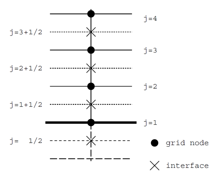
Figure 1: Boundary points dissipation [4].

7.5 Periodic Boundary Condition

A periodic condition is implemented between the first ($K=1$) and the last point in the azimutal direction ($K=K_{MAX}$) in order to close the 3-D computational domain. There are no boundaries in this direction, since all the points are inside the domain. The first and the last points, in the azimuthal direction, are superposed in order to facilitate the boundary condition implementation which is given by

$$(\rho)_{i,j,K_{MAX}} = (\rho)_{i,j,1}\,\mbox{,}$$

$$(u)_{i,j,K_{MAX}} = (u)_{i,j,1}\,\mbox{,}$$

$$(v)_{i,j,K_{MAX}} = (v)_{i,j,1}\,\mbox{,}$$ (96)

$$(w)_{i,j,K_{MAX}} = (w)_{i,j,1}\,\mbox{,}$$

$$(e)_{i,j,K_{MAX}} = (e)_{i,j,1}\,\mbox{.}$$

8 Mesh Generation

A structured mesh generator is created in order to provide CGNS grid files for the simulations performed in the present work. Figure 2(a) illustrates a frontal view of a representative domain for the jet flow simulations. The blue boundary is the freestream region and the red one is the entrance of the jet flow. The complete 3-D mesh is created by rotating a 2-D mesh around the horizontal direction, $x$. A view of this 2-D mesh is illustrated in Fig. 2(b). This approach generates a singularity at the centerline of the domain. The treatment of this region is discussed in the boundary conditions section. The authors chose not to include the nozzle geometry and the jet entrance is located at $x=0$, between $|r|/d\leq 0.5$, where $|r|$ is the distance from the centerline in the radial direction and $d$ is the incoming jet diameter. In Fig. 2(b), two distinct regions are visible: the developing region for $x/d<20$ and the fully-developed region where the flow is self-similar. In the latter, the shear layer has a constant growth rate given by $\mathcal{S}\approx 0.094$ [25]. This trend is typical of jet flows and the mesh refinement follows this evolution. The refinement is made using hyperbolic tangent functions, with a finest grid resolution near the jet entrance and along the slip line of the jet. The mesh is coarsened in the far field in order to diffuse the acoustic waves and avoid reflections at the farfield domain boundaries.

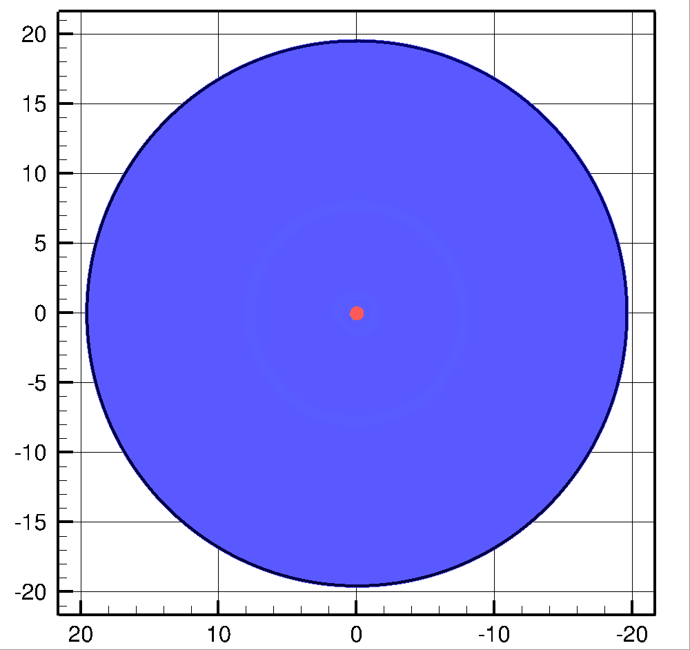
(a) Frontal view of the computational domain for the jet flow simulation

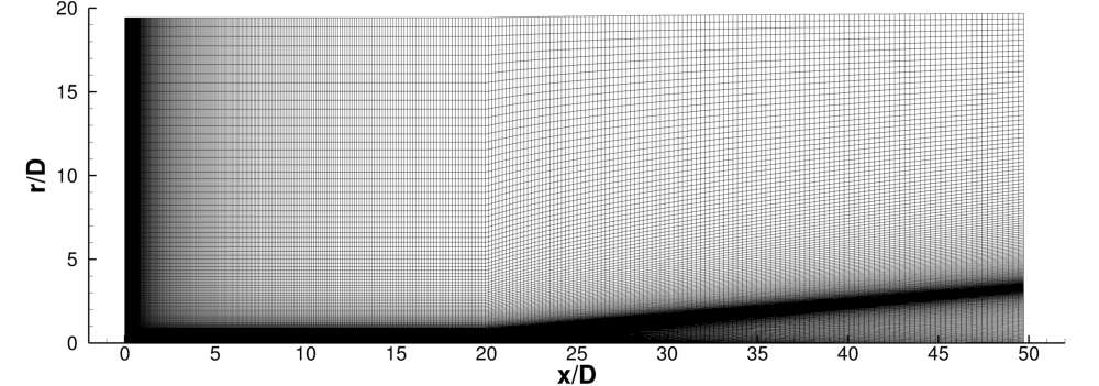
(b) 2-D view of the mesh generation.

Figure 2: Computational domain and mesh for a jet flow simulation

9 High Performance Computing

9.1 Code Parallelization and Improvements

The developement of a 3-D finite-difference numerical code within the IAE CFD group was initiated in 1997 [26, 27, 28]. In the sequence, viscous terms, multigrid techniques, implicit residual smoothing and turbulence modeling were also added to the solver [4]. As previously discussed, large eddy simulations demand very dense grids. Therefore, one can state that LES is only possible throught multi-processing computing. The authors have invested significant efforts to improve the outdated numerical solver toward a more sophisticated computational level. The FORTRAN 77 programming language was replaced by the FORTRAN 90 standard and dynamic memory allocation is included in the new version. These improvements are performed in order to simplifly the code structure and to enable the implementation of parallel computation routines.

Pre-processing and post-processing procedures are very important steps of computer-aided engineering. The original version did not have an input/output standard accepted by the vizualisation tools used by the scientific community. Hence, the CFD general notation system, also know by the CGNS [29, 30] acronym, is implemented in the present work. The main post-processing and visualization tools accept the CGNS standard.

The mesh partitioning is performed when the simulation begins. One dimensional and two dimensional partitionings are performed in the present work. The former partitionates the domain in the axial direction or the azimuthal direction and the latter partitionates the domain in both, the axial and azymuthal directions. Figure 3 illustrates the 1-D partitioning procedure in the axial direction. Each processor reads the complete domain and performs the segmentation. The partition numeration starts at zero to be consistent with the message passing interface notation which applies the C# programming language vector standard. This direction, in the general curvilinear coordinate system adopted in the present work, is the $\xi$ direction for axial partitionig and $\zeta$ for the azimuthal partitioning.

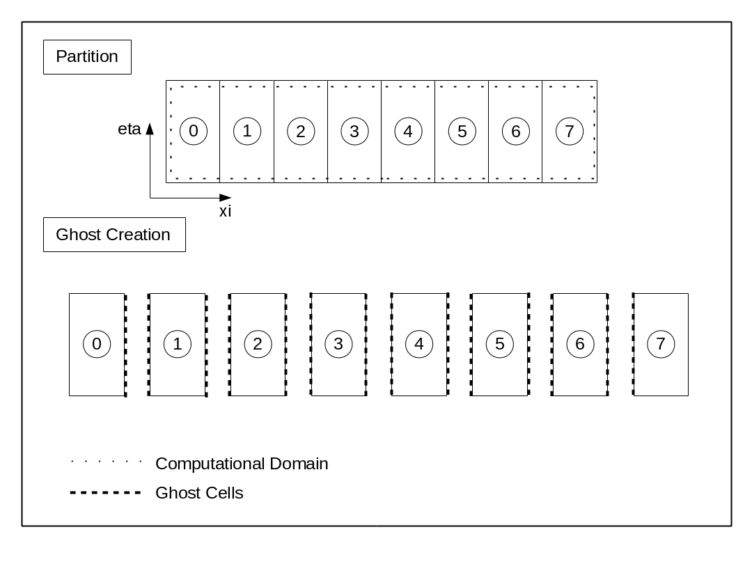
Figure 3: One dimensional mesh partitioning procedure in the axial direction.

Numerical data exchange between the partitions is necessary regarding parallel computation. In the present work, the ghost concept is applied. Ghost points are added to the local partition at the main flow direction and azimuthal direction in order to carry information of the neighboring points. The artificial dissipation scheme implemented in the code [22] uses a five points stencil which demands information of the two neighbors of a given mesh point. Hence, a two ghost-point layer is created at the beginning and at the end of each partition.

After the partitioning and the ghost cell creation, each processor performs the computation. Communication between pairs of partition neighbors are performed in order to allow data information pass through the computational domain. For each direction, the data exchange is performed in four blocking steps. Figures 4(a) and 4(b) demonstrate the 1-D communication which initially is performed in the forward direction. Even partitions send information of their two last local layers to the ghost points at the left of odd partitions. If the last partition is even, it does not share information in this step. In the sequence, odd partitions send information of their two last local layers to the ghost points at the left of even partitions. If the last partition is odd, it does not share information in this step. The third and the fourth steps are backward communications. First, odd partitions send data of their two first local layers to the ghost points at the right of even partitions. Finally, all even partitions, but the first one, send data of their two first local layers to the ghost points at the right of odd partitions.

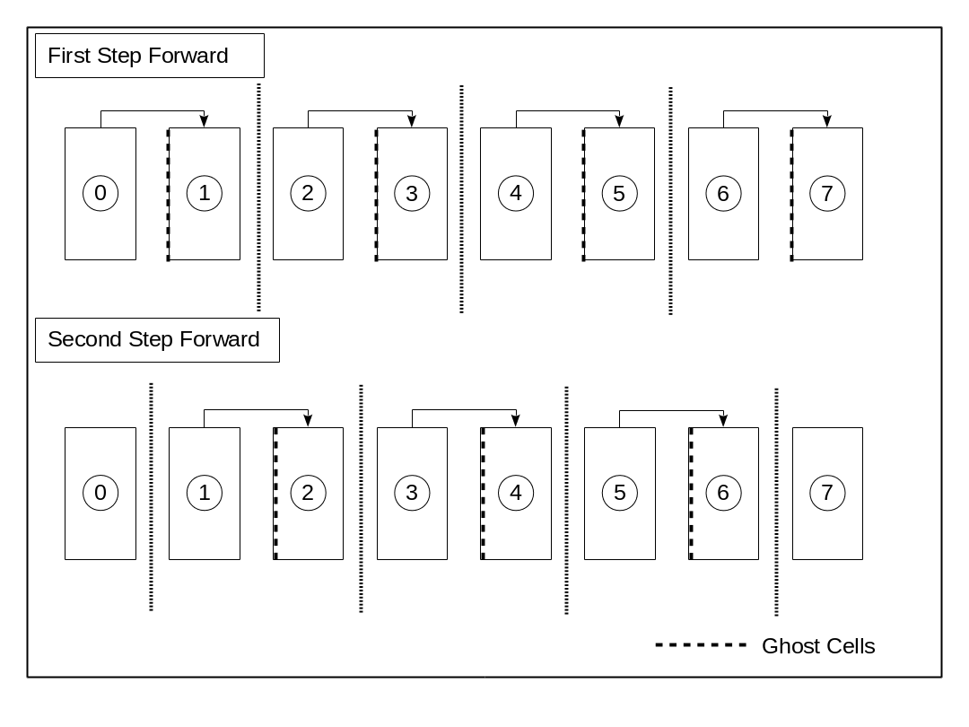
(a) Forward communication between 1-D partitions.

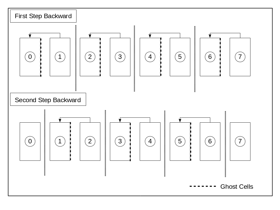
(b) Backward communication between 1-D partitions.

Figure 4: 1-D communication between partitions.

The extention to the 2-D communication is straightforward. Figures 5(a) and 5(b) illutrate the 2-D segmentation and mapping of the domain. The numeration of each partition is performed using a matrix index system in which the rows represent the position in the axial direction and the columns represent the position in the azimuthal direction. NPX and NPZ denote the number of partitions in the axial and azimuthal directions, respectively. The 2-D communication is performed first in the azimuthal direction and, then, in the axial direction in the same fashion as the 1-D data exchange is performed.

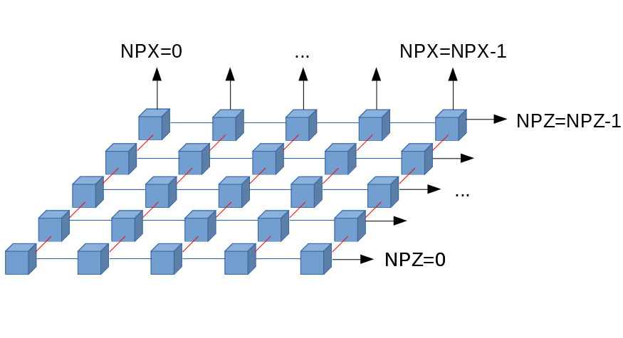
(a) 2-D partitioning in the axial and azimuthal direction.

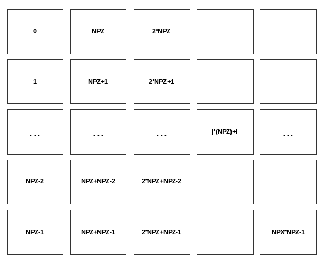
(b) Mapping of the 2-D communication.

Figure 5: 2-D partitioning and mapping.

The user can choose the frequency in which the solution is written in a CGNS file. After a chosen number of iterations, the main processor collects the data from all other processors and appends the solution to the CGNS file in a time-dependent fashion. Therefore, after the simulation, it is possible to recover the solution as a function of the physical time. However, despite the advantages, the output approach, in which one processor collects data of all other processors, is a serial output and, consequently, it can reduce the parallel computational performance. CGNS provides parallel I/O software which needs to be implemented in the future.

9.2 Computational Performance Assessment

Parallel computations can largely decrease the time of CFD simulations. However, high performance computing upgrade of a serial solver must be carefully performed. The parallel version of a solver ought to produce exactly the same results as the single processed version. Moreover, the communication between partitions is not free and can affect the computational performance in parallel. The partitioning of the domain increases the amount of communication between processors which can race with the time spent on computation and, consequently, deteriorate the performance of the solver.

The speedup is one of the most common figures-of-merit for the performance evaluation of parallel algorithms and architectures [31] and it is used in the present work in order to measure the computational efficiency of the parallel solver and compare with the ideal case. Different approaches are used by the scientific community in order to calculate the speedup [32, 33]. In the present work, the speedup, ${Sp}_{N}$, is calculated as

$${Sp}_{N}=\frac{T_{N}}{T_{s}}\,\mbox{,}$$ (97)

in which $T_{N}$ and $T_{s}$ stand for the time spent to perform one thousand iterations using $N$ processors and one single processor, respectively. The efficiency as a function of the number of processors, $\eta_{N}$, is written considering Amdahl’s law [34] as

$$\eta_{N}=\frac{{Sp}_{N}}{N}\,\mbox{.}$$ (98)

Gustafson [32] has discussed that the efficiency of a parallel task scales with the size of the problem. Therefore, different meshes are created in order to evaluate the performance of the solver as a function of the number of points within partitions. Table 1 presents the mesh size and the number of points in the three directions of the domain, $n_{\xi}$, $n_{\eta}$ and $n_{\zeta}$.

Table 1: Mesh information

Mesh	$n_{\xi}$	$n_{\eta}$	$n_{\zeta}$	Mesh size	Mesh	$n_{\xi}$	$n_{\eta}$	$n_{\zeta}$	Mesh size
1	200	150	40	1.20E06	6	400	150	10	6.00E05
2	400	150	40	2.4E06	7	400	150	60	3.60E06
3	800	150	40	4.80E06	8	800	300	120	2.88E07
4	400	75	40	1.20E06	9	200	75	40	6.00E05
5	400	300	40	4.80E06	10	200	75	20	3.00E05

The ratio of computation-communication costs per partition is measured in the present work regarding the evaluation of the best partitioning arrangement for the solver. Only the 1-D partitioning in the axial direction is evaluated in the present work. The ratio is proportional to the number of points in the main flow direction, $n_{\xi}$. This statement is true because the computational cost of a partition is directly related to the size of the domain and the communication cost is directly related to the number of ghost-points of each partition which, for the present 1-D axial partitioning, is proportional to the number of points in the radial direction times the number of points in the azimuthal direction.

A simplified flow simulation was performed using the meshes presented in Tab. 1 and different number of processors. The speedup and efficiency of the solver is presented in Tab. 2. In this table, $N$ represents the number of processors used in each test case. Figures 6(a) and 6(b) illustrate the trends for the evolution of speedup and efficiency as a function of the number of processors. In these figures, the symbols indicate the actual speedup and efficiency values obtained in the various tests, whereas the curves represent the trends given by least-squares best fits through the data. One can state that the code has the best computational performace for $n_{\xi}>50$. The efficiency is $\mathcal{O}(1)$ for all configurations with $n_{\xi}>50$ presented in this section. For $40<n_{\xi}<50$, the communication costs become significant and begin to deteriorate the performance, which decreases even further with smaller partition sizes. For $n_{\xi}\approx 5$ the communication is more expensive than computation. The speedup coefficient is higher for configurations with $n_{\xi}\approx 10$ than configurations with $n_{\xi}\approx 5$. The results motivated the extention to a 2-D partitioning in the code. However, the scalability for such partition configurations was not measured for the the current paper.

Table 2: Table of speedup and efficiency as a function of the number of processors

Mesh Nb.
1	$N$ 2 5 8 10 15 20 40 $S_{N}$ 1.937 4.768 7.858 8.165 11.35 12.00 10.95 $\eta_{N}$ 0.969 0.953 0.982 0.816 0.756 0.600 0.274 $n_{\xi}$ 100 40 25 20 13 10 5
2	$N$ 2 5 8 10 15 20 40 $S_{N}$ 2.030 4.338 9.125 9.265 11.62 14.15 15.23 $\eta_{N}$ 1.015 0.868 1.141 0.926 0.775 0.708 0.381 $n_{\xi}$ 200 80 50 40 26 20 10
3	$N$ 2 5 8 10 15 20 40 $S_{N}$ 2.644 5.021 10.51 12.02 19.00 20.64 23.75 $\eta_{N}$ 1.322 1.004 1.314 1.212 1.266 1.032 0.594 $n_{\xi}$ 400 160 100 80 53 40 20
4	$N$ 2 5 8 10 15 20 40 $S_{N}$ 2.406 4.718 8.632 10.02 13.04 15.40 15.62 $\eta_{N}$ 1.203 0.944 1.079 1.002 0.869 0.770 0.390 $n_{\xi}$ 200 80 50 40 26 20 10
5	$N$ 2 5 8 10 15 20 40 $S_{N}$ 2.030 4.909 9.124 9.257 11.55 14.13 15.17 $\eta_{N}$ 1.015 0.982 1.140 0.926 0.770 0.706 0.379 $n_{\xi}$ 200 80 50 40 26 20 10
6	$N$ 2 5 8 10 15 20 40 $S_{N}$ 2.141 3.703 7.461 8.648 10.88 13.06 14.22 $\eta_{N}$ 1.070 0.741 0.933 0.865 0.725 0.653 0.355 $n_{\xi}$ 200 80 50 40 26 20 10
7	$N$ 2 5 8 10 15 20 40 $S_{N}$ 2.300 4.916 8.393 9.599 12.60 14.24 14.15 $\eta_{N}$ 1.150 0.983 1.050 0.960 0.840 0.712 0.354 $n_{\xi}$ 200 80 50 40 26 20 10
8	$N$ 2 5 8 10 15 20 40 $S_{N}$ 2.140 5.441 9.730 9.762 20.27 20.30 22.84 $\eta_{N}$ 1.070 1.088 1.216 0.973 1.352 1.015 0.571 $n_{\xi}$ 400 160 100 80 53 40 20
9	$N$ 2 5 8 10 15 20 40 $S_{N}$ 1.915 4.482 6.585 7.576 9.838 10.66 10.37 $\eta_{N}$ 0.957 0.896 0.823 0.758 0.656 0.530 0.259 $n_{\xi}$ 100 40 25 20 13 10 5
10	$N$ 2 5 8 10 15 20 40 $S_{N}$ 2.319 4.953 8.480 9.768 12.52 14.29 15.29 $\eta_{N}$ 1.116 0.990 1.060 0.977 0.835 0.714 0.382 $n_{\xi}$ 100 40 25 20 13 10 5

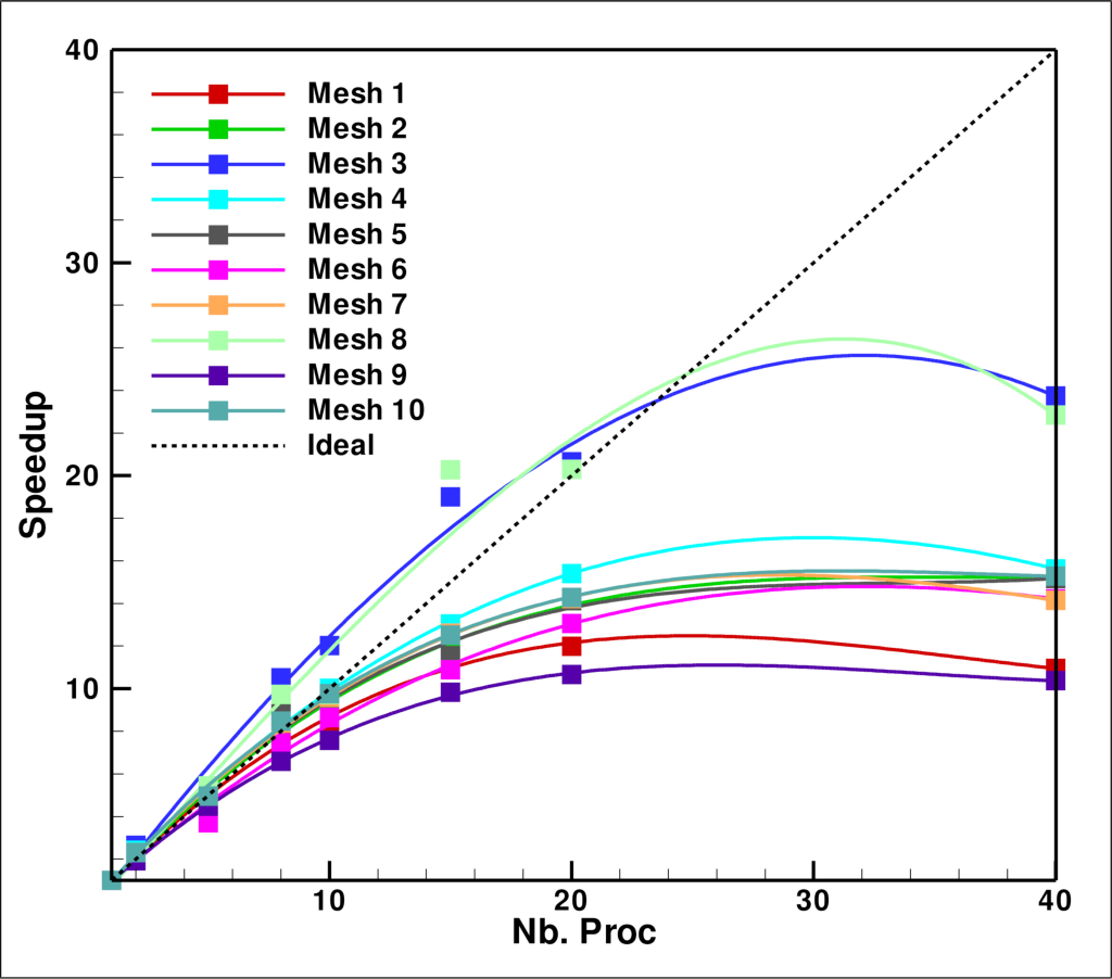
(a) Speedup as a function of the number of processors.

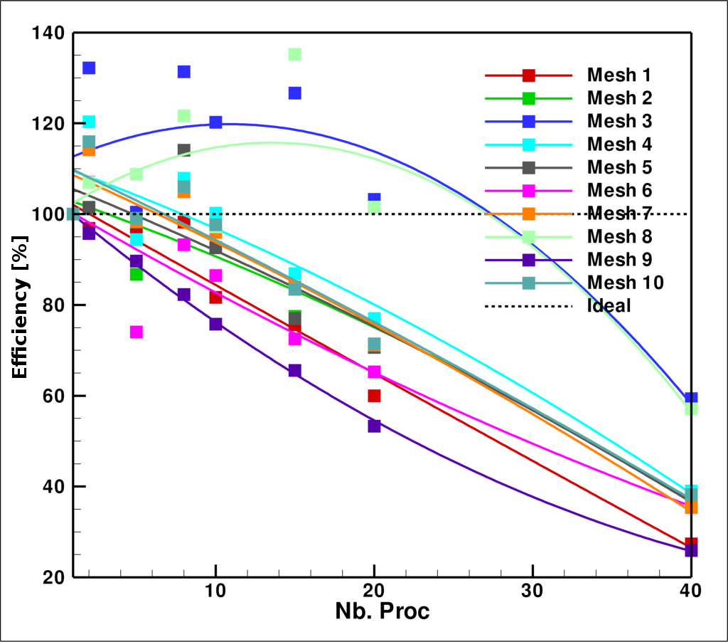
(b) Efficiency as a function of the number of processors.

Figure 6: Trends observed for speedup and computational efficiency of the parallel version of the code.

The binary reproducibility of the solver was also evaluated in the present work. A high performance computing code must produce exactly the same results as the serial version of the code, regardless of the number of processors used. Therefore, three large eddy simulations of jet flows were performed using a single processor, 1-D partitioning in the axial direction and 1-D partitioning in the azimuthal direction. Figure 7 illustrates the history of maximum absolute value of the right-hand side of the continuity equation through 1500 iterations. In other words, the figure is showing what would be the $L_{\infty}$ norm of the residue of the continuity equation if these were standard steady state calculations. The goal is the evaluation of differences between serial and parallel configurations. Visually, all the three simulations present the same behavior, independently of the number of processors. However, only the partitioning in the axial direction presents binary reproducibility compared the serial simulation. The azimuthal partitioning has accumulated differences on fifth significant figure at the end of the 1500 iterations. This is due to the fact that MPI collective communications have to be performed in the azimuthal direction in order to average properties at the centerline. Floating-point operations, such as sums and products, are commutative and not associative. Thus, the order in which they are performed makes a difference to the final outcome [35], and, for each azimuthal partitioning configuration, the result of the average at the centerline is different in the context of bitwise reproducibility.

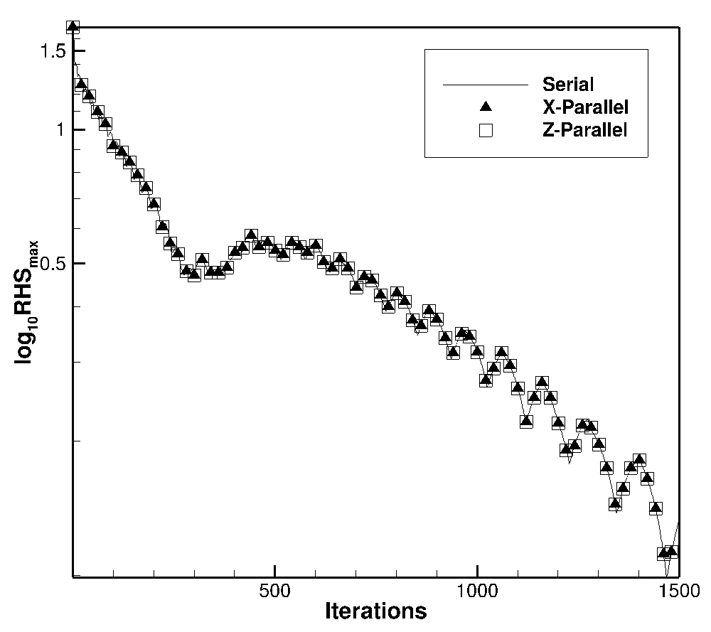
Figure 7: Maximum RHS of large eddy simulations of jet flows using different partitioning.

10 Numerical Results

The present section is devoted to a preliminary study of a supersonic perfectly expanded jet flow. Results are compared with analytical, numerical and experimental data from the literature [1, 8, 9, 10, 36, 37]. First LES results using the Smagorinsky SGS turbulence closure [6] are discussed. The flow is characterized by an unheated perfectly expanded inlet jet with a Mach number of $1.4$ at the domain entrance. Therefore, the pressure ratio, $PR=P_{j}/P_{\infty}$, and the temperature ratio, $TR=T_{j}/T_{\infty}$, between the jet exit and the ambient freestream are equal to one, $PR=1$ and $TR=1$. The time step used in the simulation is constant and equal to $2.5\times 10^{-5}$ in dimensionless form. The Reynolds number of the jet is $Re=1.57\times 10^{6}$. The radial and longitudinal dimensions of the smallest cell of the computational domain are given by $(\Delta\underline{r})_{min}=0.002$ and $(\Delta\underline{x})_{min}=0.0126$, respectively, again in dimensionless form. This cell is located in the shear layer of the jet, at the entrance of the computational domain. The number of points in the azimuthal direction is $N_{\theta}=180$. The mesh domain is composed by 14.4 million points. The present mesh reproduces well the main geometric characteristics of the reference grid[8].

Generally, compressible jet flow studies performed in the literature present mean field properties. However, as the present simulation is not statistically converged yet, mean quantities could not be calculated. As an example, using the same flow configuration, Mendez[8] needed 300 characteristic times, $\mathcal{T}_{\infty}$, to obtain averages. Here, $\mathcal{T}_{\infty}$ is defined as the ratio between the diameter D and the ambient sound speed $a_{\infty}$. The simulation time of the cited reference corresponds approximatively to four flow through times. One flow through time is the time for a particle to cross the entire domain from the jet entrance to the domain exit. The reader should remember that, as $TR=1$ and $a_{j}=a_{\infty}$, the characteristic time in the present work is equal to that reported in the work of Mendez [8]. In the present work, the code assessment of the supersonic jet flow is made by observing the last obtained snapshot. This snapshot corresponds to 18.5 $\mathcal{T}_{j}$ which is far less than the computational time in the reference. However, the authors chose to start the analysis of the jet flow using this field. Figure 8 displays instantaneous fields of pressure and vorticity of the jet at that instant. The jet is entering into the domain at the left and evolves towards the right of the domain. As the flow has been initialized from stagnation conditions and not, for instance, from a converged RANS solution, a front pressure shock wave is preceding the first vortical structures. Figure 8 focuses on the jet flow entrance. At the beginning of the mixing layer, thin axisymmetrical vortices are growing and pairing, leading then to turbulent transition at approximatively $x=1.5D$. This figure also displays Mach waves emitted by the mixing layer, displaying a downstream directivity, retrieving traditional trends [1, 8, 9, 10, 36, 37]. One can notice that the strongest acoustic sources match the coherent structure locations, identifiable by the condensed vorticity rings.

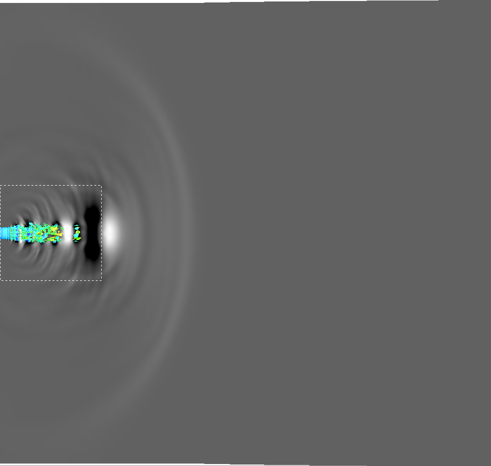
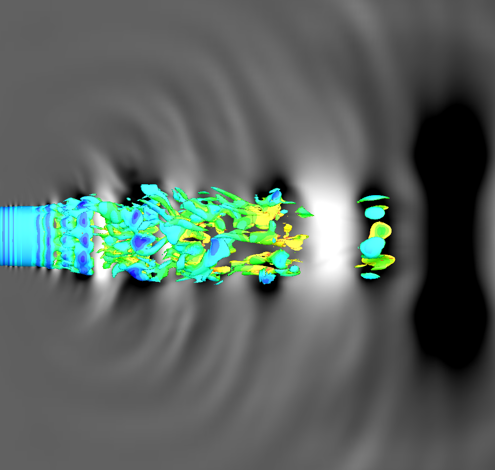
Figure 8: Instantaneous pressure and vorticity fields for the perfectly expanded supersonic jet. The gray scale contours show $\underline{p}$ from 0.4 to 0.9, while a dimensionless iso-contour of vorticity of magnitude $|\omega|D/U_{j}=10$ is colored by the streamwise velocity $\underline{u}$ from -0.2 (blue) to 1.4 (red).

Figure 9 presents the radial profile of the streamwise velocity component at $x=2.5D$ and compares it with the averaged numerical and experimental profiles from Mendez[8] and Bridges[10], respectively. The centerline values of the velocity profile are overestimated in the current simulation when compared to the references. This difference is expected since a flat inlet boundary profile is used for this simulation while a laminar profile, necessarily thicker, is used in the numerical reference work. However, keeping in mind that the current profile is instantaneous, a fair agreement is obtained. Similar observations can be made on the results comparing the centerline streamwise velocity components, shown in Figure 9. The values in the potential core, corresponding to the jet area until $U=0.95\cdot U_{j}$, compare well with the references. Moreover, one can expect that, as the jet will grow downstream, the decreasing slope after the potential core will raise to meet the reference curves, confirming thus the good trend of the present simulation.

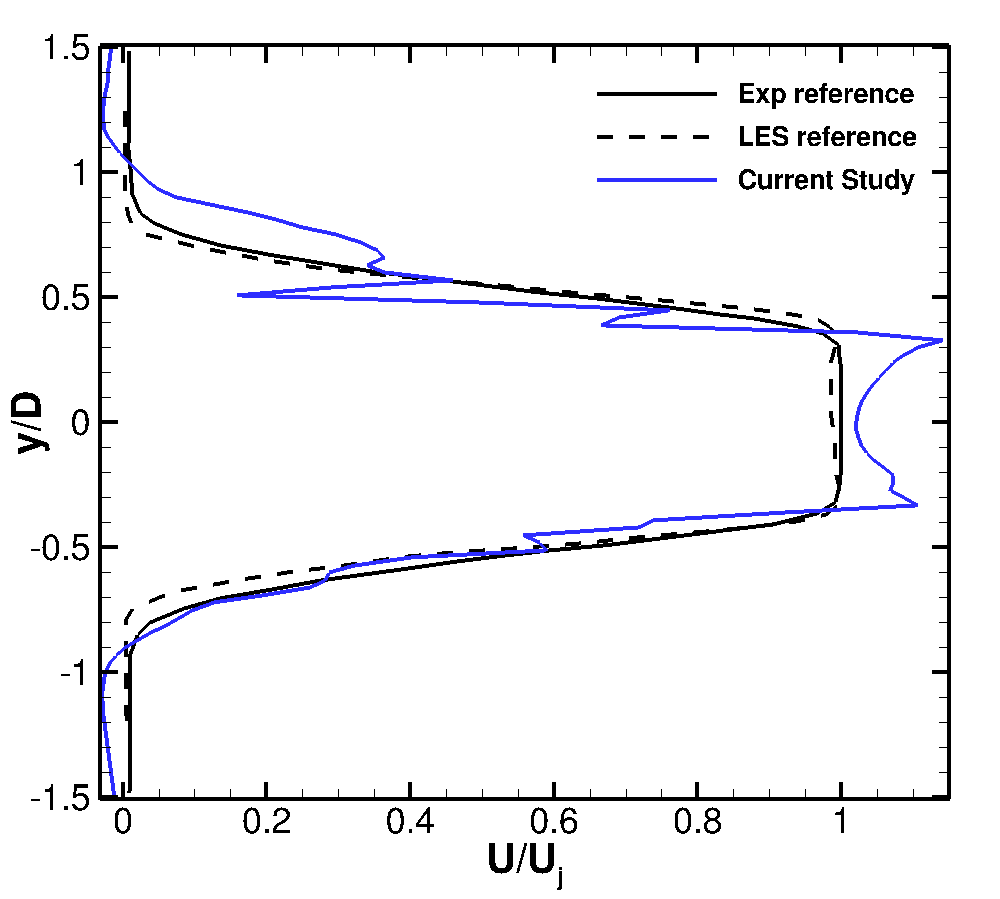
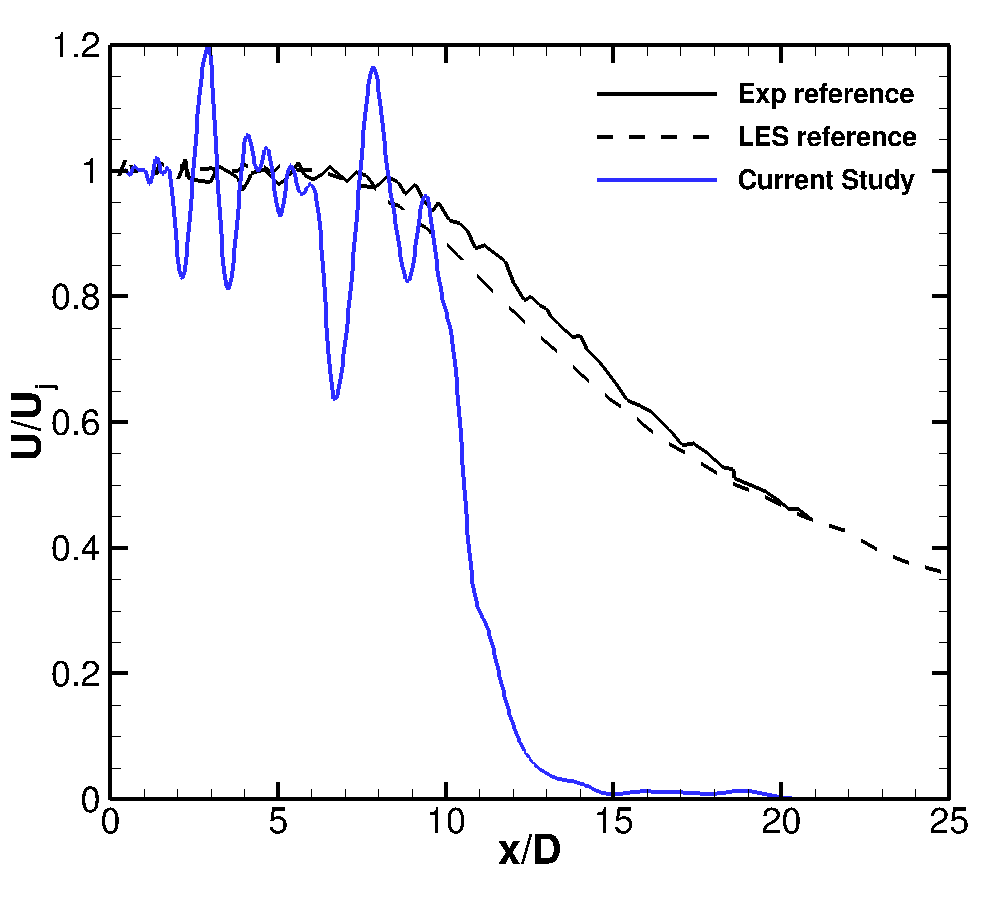
Figure 9: Comparison between numerical and experimental streamwise velocity component profiles along the centerline ($a$), and radial profiles at $x=2.5D$. Instantaneous results from the present study are compared with LES results[8] and experimental ones[10].

Another visualization of this jet flow is shown in Figure 10. It is possible to observe the evolution of the vorticity looking at different cross-flow planes from $\underline{x}=0.1$ to $7.5$. At the moment of this snapshot, slices located after the last streamwise position shown are irrelevant as the jet is not fully developed yet. From $\underline{x}=0.1$ to 0.25, the mixing layer is getting thicker and it is axisymmetric as already observed in Figure 8. Further downstream, the flow becomes completely three dimensional and is no longer axisymmetric, transitioning towards a turbulent state. Still, the turbulent vortical structures are larger than already observed in the literature[8, 38]. This is due to the low order of the computational code and the barely acceptable refinement of the grid for LES simulations. The mixing layer continues widening as one moves downstream. One can clearly expect that the mixing layer will spread until the jet centerline near the end of the potential core.

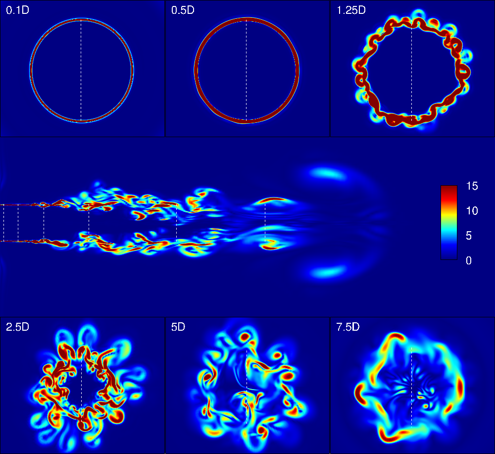
Figure 10: Instantaneous vorticity magnitude for the present simulation at $M=1.4$.

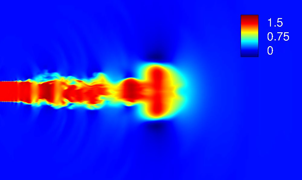
(a) $\underline{u}$

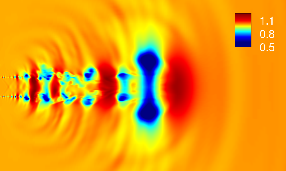
(b) $\underline{\rho}$

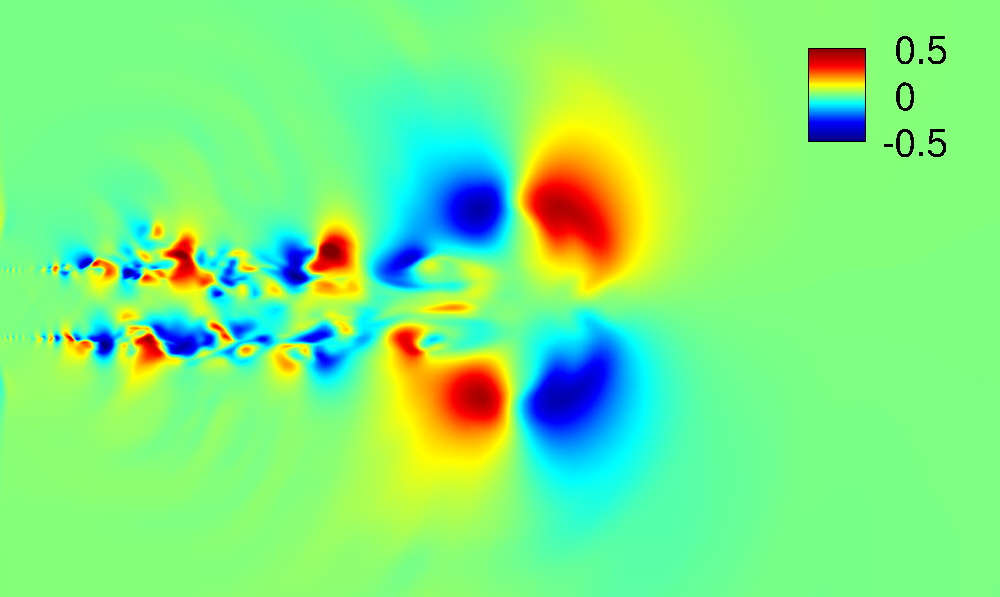
(c) $\underline{v}$

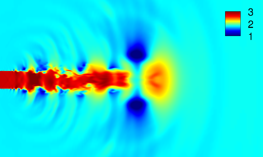
(d) $\underline{E}$

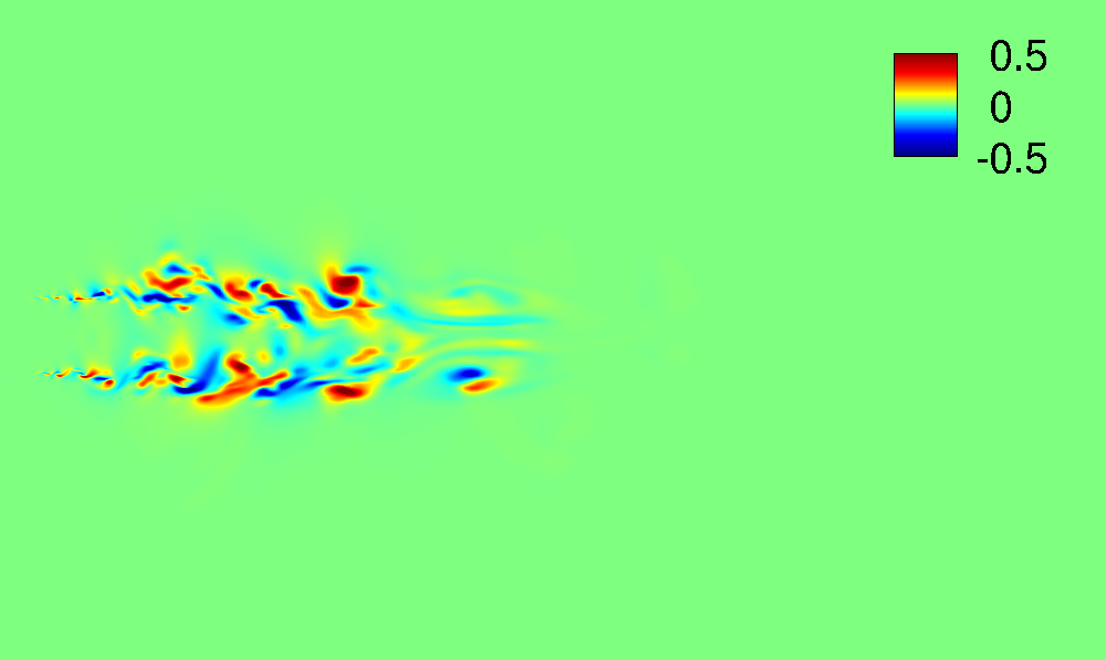
(e) $\underline{w}$

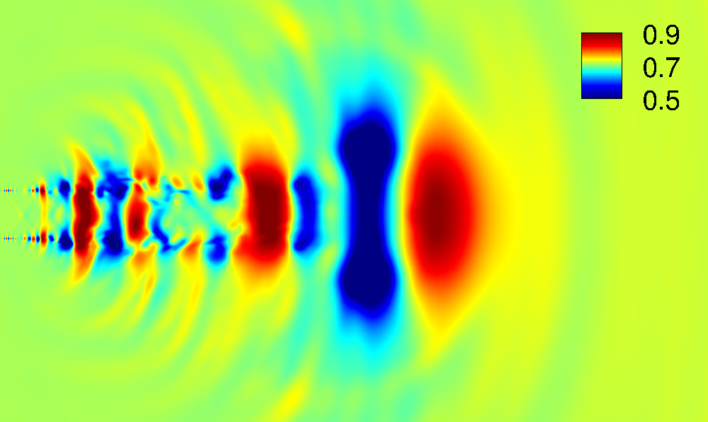
(f) $\underline{p}$

Figure 11: Instantaneous properties of the perfectly expanded supersonic jet flow.

Finally, flow properties are displayed in Figure 11. In this two dimensional snapshot, radial and azimuthal velocity components correspond to vertical and spanwise velocity components, respectively. The $\underline{v}$ and $\underline{w}$ velocity components are of the same order of magnitude in the jet mixing layer turbulent region, illustrating thus the three dimensional turbulent behaviour of the jet mixing layer. Looking at the second column of Figure 11, one can observe weak shock cells in the instantaneous density, total energy and pressure fields. Downstream directivity patterns are very similar to those seen in the reference work [8, 38], confirming one more time that the current simulation is evolving towards the correct trends.

11 Concluding Remarks

The current work is based on the development of novel large eddy simulation tool for the study of supersonic jet flows. The numerical code background is a RANS solver designed for rocket flow configurations. The original solver is improved in order to simulate supersonic jet flows using an LES formulation within a multiprocessor environment.

Parallel and serial simulations are performed in order to validate the reproducibility of the code. Two different approaches are used to partitionate the computational domain for the parallel simulation. One partitioning is performed in the axial direction and the other one in the azimuthal direction. All simulations have produced similar results. However, binarywise reproducibility was only achieved for the axial partitioning. There are differences on the last significant figure for the azimuthal partitioning. The centerline condition demands the use of collective MPI communication when the azimuthal partitioning is performed. Such communications can destroy the binarywise reproducibility of the solver. Efforts are being taken in order to solve the issue without impacting the performance of the parallel solver. The 1-D computational efficiency in the axial direction of the parallel code, using different numbers of processors, is also assessed and discussed. The code has presented linear speedups for partition width with more than 50 points in the flow direction. This behavior is expected since the communication between partitions starts to race against computation for smaller domains. However, due to the large size of the problem, the 2-D partitioning strategy has been used for all LES calculations here.

Large eddy simulations of a perfectly expanded supersonic jet flow configuration are performed. The classical Smagorinsky model is used to calculate the subgrid terms. Results obtained in this work do not allow the calculation of statistically time-averaged properties since the simulation only ran during a very limited time period. However, since the aim of the paper is mostly to validate the LES computational tool, the authors believe that the results here included should provide enough information to allow evaluation of the trends of jet physics. Early quantitative comparisons with numerical [8] and experimental [10] reference work are obtained. The jet mixing layer is showing strong instabilities evolving towards a turbulent state. The classical downstream directivity pattern already observed in the literature [1, 8, 9, 10, 37] is retrieved. The velocity profiles also show a good agreement with the references.

Finally, regarding the low order, more dissipative numerical scheme, the early results show a fairly good agreement with the references, indicating that grid refinement could probably resolve such issues. Hence, for future simulations, a much more refined new grid should be used to counterbalance the dissipation induced by the numerical scheme. In addition, the computational code needs to be further improved through the availability of more sophisticated time-marching schemes. For instance, the time step used in the present simulations is one hundred times smaller than the one used in literature [8], leading to a prohibitive simulation cost. Hence, a new time integration method should be implemented, such as a preconditioned dual-time step procedure [39]. Furthermore, acoustic predictions of the far field noise using the Ffowcs Williams and Hawkings analogy will be performed using the reference work of Wolf et al.[40]. Results will be compared one more time with the numerical studies of Mendez et al.[8], Brès et al.[38] and Khalighi et al.[41]. The influence of the inlet boundary profile on the acoustics will also be investigated.

References

- [1] Bodony, D. and Lele, S. K., “On Using Large-Eddy Simulation For the Prediction of Noise From Cold and Heated Turbulent Jets,” Physics of Fluids, Vol. 17, No. 8, Aug. 2005.
- [2] Garnier, E., Adams, N., and Sagaut, P., Large Eddy Simulation for Compressible Flows, Springer, 2009.
- [3] Wolf, W. R., Azevedo, J. L. F., and Lele, S. K., “Convective Effects and the Role of Quadrupole Sources for Aerofoil Aeroacoustics,” Journal of Fluid Mechanics, Vol. 708, 2012, pp. 502–538.
- [4] Bigarella, E. D. V., Three-Dimensional Turbulent Flow Over Aerospace Configurations, M.Sc. Thesis, Instituto Tecnológico de Aeronáutica, São José dos Campos, SP, Brasil, 2002.
- [5] Vreman, A. W., Direct and Large-Eddy Simulation of the Comperssible Turbulent Mixing Layer, Ph.D. thesis, Universiteit Twente, 1995.
- [6] Smagorinsky, J., “General Circulation Experiments with the Primitive Equations: I. The Basic Experiment,” Monthly Weather Review, Vol. 91, No. 3, March 1963, pp. 99–164.
- [7] Eidson, T. M., “Numerical Simulation of the Turbulent Rayleigh–Bénard Problem Using Subgrid Modelling,” Journal of Fluid Mechanics, Vol. 158, 1985, pp. 245–268.
- [8] Mendez, S., Shoeybi, M., Sharma, A., Ham, F. E., Lele, S. K., and Moin, P., “Large-Eddy Simulations of Perfectly-Expanded Supersonic Jets: Quality Assessment and Validation,” AIAA Paper No. 2010–0271, January 2010.
- [9] Tanna, H. K., “An Experimental Study of Jet Noise Part I: Turbulent Mixing Noise,” Journal of Sound and Vibration, Vol. 50, No. 3, 1977, pp. 405–428.
- [10] Bridges, J. and Wernet, M. P., “Turbulence Associated with Broadband Shock Noise in Hot Jets,” AIAA paper, Vol. 2834, 2008, pp. 2008.
- [11] Boussinesq, M. J., “Essai sur la Théorie des Eaux Courantes,” In: Mémoires Présentés par Divers Savants à l’Academie des Sciences, tome XXIII, Imprimerie Nationale, 1877, pp. 43–47.
- [12] Erlebacher, G., Hussaini, M. Y., Speziale, C. G., and Zang, T. A., “Toward the Large-Eddy Simulation of Compressible Turbulent Flows,” Journal of Fluid Mechanics, Vol. 238, 1992, pp. 155–185.
- [13] Lilly, D. K., “On the Computational Stability of Numerical Solutions of Time- Dependent Non-Linear Geophysical Fluid Dynamics Problems,” Monthly Weather Review, Vol. 93, No. 1, January 1965, pp. 11–25.
- [14] Lilly, D. K., “The Representation of Small-Scale Turbulence in Numerical Simulation Experiments,” IBM Form No. 320-1951, Proceedings of the IBM Scientific Computing Symposium on Environmental Sciences, Yorktown Heights, N.Y., 1967, pp. 195–210.
- [15] Moin, P., Squires, K., Cabot, W., and Lee, S., “A Dynamic Subgrid-Scale Model for Compressible Turbulence and Scalar Transport,” Physics of Fluids A: Fluid Dynamics (1989-1993), Vol. 3, No. 11, 1991, pp. 2746–2757.
- [16] Martín, M. P., Piomelli, U., and Candler, G. V., “Subgrid-Scale Models for Compressible Large-Eddy Simulations,” Theoretical and Computational Fluid Dynamics, Vol. 13, No. 5, 2000, pp. 361–376.
- [17] Lenormand, E., Sagaut, P., Phuoc, L. T., and Comte, P., “Subgrid-Scale Models for Large-Eddy Simulations of Compressible Wall Bounded Flows,” AIAA Journal, Vol. 38, No. 8, 2000, pp. 1340–1350.
- [18] Coleman, G. N., Kim, J., and Moser, R. D., “A Numerical Study of Turbulent Supersonic Isothermal-Wall Channel Flow,” Journal of Fluid Mechanics, Vol. 305, 1995, pp. 159–183.
- [19] Lesieur, M., Turbulence in Fluids, Springer, Saint Martin d´Hères, France, 4th ed., 2008.
- [20] Larchêveque, M. L., Simulation des Grandes Échelles de l‘Écoulement Au-Dessus d‘une Cavité, Ph.D. thesis, Université Paris VI - Pierre et Marie Curie, Paris, France, December 2003.
- [21] Turkel, E. and Vatsa, V. N., “Effect of Artificial Viscosity on Three-Dimensional Flow Solutions,” AIAA Journal, Vol. 32, No. 1, 1994, pp. 39–45.
- [22] Jameson, A. and Mavriplis, D., “Finite Volume Solution of the Two-Dimensional Euler Equations on a Regular Triangular Mesh,” AIAA Journal, Vol. 24, No. 4, Apr. 1986, pp. 611–618.
- [23] Jameson, A., Schmidt, W., and Turkel, E., “Numerical Solutions of the Euler Equations by Finite Volume Methods Using Runge-Kutta Time-Stepping Schemes,” AIAA Paper 81–1259, Proceedings of the AIAA 14th Fluid and Plasma Dynamic Conference, Palo Alto, Californa, USA, June 1981.
- [24] Long, L. N., Khan, M., and Sharp, H. T., “A Massively Parallel Three-Dimensional Euler/Navier-Stokes Method,” AIAA Journal, Vol. 29, No. 5, 1991, pp. 657–666.
- [25] Pope, S. B., Turbulent Flows, Cambridge University Press, Cambridge, UK, 2000.
- [26] Vieira, R., Azevedo, J. L. F., and Fico Jr., N. G. C. R., “Slotted Transonic Wind Tunnel Flow Simulations Using the Euler Equations,” Proceedings of the 14th Brazilian Congress of mechanical Engineering – COBEM 97, Bauru, SP, Brazil, Dec. 1997.
- [27] Vieira, R., Azevedo, J. L. F., Fico Jr., N. G. C. R., and Basso, E., “Three Dimensional Simulations of the Flow in a Slotted Transonic Wind Tunnel,” Proceedings of the 10h International Conference on Finite Element Methods, Tucson, AZ, USA, Jan. 1998, pp. 431–436.
- [28] Vieira, R., Azevedo, J. L. F., Fico Jr., N. G. C. R., and Basso, E., “Three Dimensional Flow Simulation in the Test Section of a Slotted Transonic Wind Tunnel,” ICAS Paper No. 98-R.3.11, Proceedings of the 21th Congress of the International Council of the Aeronautical Sciences, Melbourne, Australia, Sept. 1998.
- [29] Piorier, D. and Enomoto, F. Y., “The CGNS System,” AIAA Paper No. 98–3007, 1998.
- [30] CGNS – CFD Data Standard, CFD General Notation System Overview and Entry-Level Documentation, Document Version 3.1.2.
- [31] Ertel, W., “On the Definition of Speedup,” PARLE’94 Parallel Architectures and Languages Europe, Springer, Berlin, 1994, pp. 289–300.
- [32] Gustafson, J. L., “Reevaluating Amdahl’s Law,” Communications of the ACM, Vol. 31, No. 5, 1988, pp. 532–533.
- [33] Sun, X.-H. and Chen, Y., “Reevaluating Amdahl’s Law in Multicore Era,” J. Parallel Distrib. Comput., Vol. 70, No. 2, Feb. 2010, pp. 183–188.
- [34] Amdahl, G. M., “Validity of the Single Processor Approach to Achieving Large Scale Computing Capabilities,” AFIPS Conference Proceedings, Vol. 30, ACM, Atlantic City, N.J., USA, Apr. 1967, pp. 483–485.
- [35] Balaji, P. and Kimpe, D., “On the Reproducibility of MPI Reduction Operations,” 2013 IEEE 10th International Conference on High Performance Computing and Communications & IEEE International Conference on Embedded and Ubiquitous Computing (HPCC_EUC), IEEE, 2013, pp. 407–414.
- [36] Lo, S. C., Aikens, K. M., Blaisdell, G. A., and Lyrintzis, A. S., “Numerical Investigation of 3-D Supersonic Jet Flows using Large-Eddy Simulation,” International Journal of Aeroacoustics, Vol. 11, No. 7, 2012, pp. 783–812.
- [37] Laufer, J., Schlinker, R., and Kaplan, R., “Experiments on Supersonic Jet Noise,” AIAA Journal, Vol. 14, No. 4, 1976, pp. 489–497.
- [38] Bres, G. A., Nichols, J. W., Lele, S. K., and Ham, F. E., “Towards Best Practices for Jet Noise Predictions with Unstructured Large Eddy Simulations,” AIAA Paper No. 2012-2965, Proceedings of the 42nd AIAA Fluid Dynamics Conference and Exhibit, New Orleans, Louisiana, June 2012.
- [39] Pandya, S. A., Venkateswaran, S., and Pulliam, T. H., “Implementation of Preconditioned Dual-Time Procedures in OVERFLOW,” AIAA Paper No. 2003-0072, Proceedings of the 41st AIAA Aerospace Sciences Meeting & Exhibit, Reno, NV, Jan. 2003.
- [40] Wolf, W. R. and Lele, S. K., “Aeroacoustic Integrals Accelerated by Fast Multipole Method,” AIAA Journal, Vol. 49, No. 7, July 2011, pp. 1466–1477.
- [41] Khalighi, Y., Ham, F., Moin, P., Lele, S. K., Colonius, T., Schlinker, R. H., Reba, R. A., and Simonich, J., “Unstructured Large Eddy Simulation Technology for Prediction and Control of Jet Noise,” ASME Turbo Expo 2010: Power for Land, Sea, and Air, American Society of Mechanical Engineers, 2010, pp. 57–70.