Quantum scars in spin-$1/2$ isotropic Heisenberg clusters

Abstract

We investigate the influence of the external fields on the statistics of energy levels and towers of eigenstates in spin-$1/2$ isotropic Heisenberg clusters, including chain, ladder, square and triangular lattices. In the presence of uniform field in one direction, the SU($2$) symmetry of the system allows that almost whole spectrum consists of a large number of towers with identical level spacing. Exact diagonalization on finite clusters shows that random transverse fields in other two directions drive the level statistics from Poisson to Wigner-Dyson (WD) distributions with different values of mean level spacing ratio, indicating the transition from integrability to non-integrability. However, for the three types of clusters, it is found that the largest tower still hold approximately even the symmetry is broken, resulting to a quantum scar. Remarkably, the non-thermalized states cover the Greenberger-Horn-Zeilinger (GHZ) and W states, which maintain the feature of revival while a Neel state decays fast in the dynamic processes. In addition, some dynamic schemes for experimental detection are proposed. Our finding reveals the possibility of quantum information processing that is immune to the thermalization in finite size quantum spin clusters.

Keywords: Quantum Scar, Quantum Thermalization, Spin dynamics, Quantum information

1 Introduction

It is commonly believed that the main obstacle for the practical realization of quantum information processing is the decoherence of the quantum state caused by interactions with the environment. However, like a thermodynamic system, where the process of thermalization always eventually destroys the information of an initial state, the thermalization is also expected to be unavoidable in a generic isolated nonintegrable quantum system. Recently, it is well established that some nonintegrable systems can fail to thermalize due to rare nonthermal eigenstates called quantum many-body scars (QMBS) [1, 2, 3, 4, 5, 6, 7, 8, 9, 10, 11, 12, 13, 14, 15, 16, 17]. These nonthermal states are typically excited ones and span a subspace, in which any initial states do not thermalize and can be back periodically. The quantum many-body scarring can prevent the thermalization starting from certain initial states. Therefore, the quantum information stored in the subspace does not dissipate at finite temperature, holding promise for potential applications in quantum information processing. The main task in this field is finding scars in a variety of nonintegrable many-body systems.

In this work, we concentrate on quantum spin-$1/2$ Heisenberg clusters, which have been successfully realized in experiments and studied under their unitary time evolution[18, 19, 20, 21, 22, 23]. In this paper, our aim is to explore the transition from integrability to non-integrability induced by external field and the possible quantum scars in a simple Heisenberg model. In the presence of uniform field $h$ in $z$ direction, the SU($2$) symmetry of an isotropic Heisenberg system allows that almost whole spectrum consists of large number of towers with identical level spacing. It has been shown that the conjecture of Anderson localization (AL)[24] can be extended to quantum spin systems by applying random field, known as many-body localization (MBL)[25, 26, 27] which preventing thermalization and even protecting quantum order[28]. Here, we study the similar quantum system, but focus on an alternative aspect. We investigate the influence of the external fields on the statistics of energy levels and towers of eigenstates in Heisenberg clusters, including chain, ladder, square and triangular lattices. Exact diagonalization on finite clusters shows that random transverse fields in $x$ and $y$ directions drive the level statistics from Poisson to Wigner-Dyson (WD) distributions with two different values of mean level spacing ratio. Numerical results show that the cooperation between the uniform field $h$ in $z$ direction, and the random field in $x$ or $y$ direction within their respective regions, takes the crucial role for the transition from integrability to non-integrability. Here we emphasize that the conclusion here is obtained only from small size systems. But the number of energy levels is large enough to count its statistics. For the three types of clusters, it is found that the largest tower still hold approximately even the symmetry is broken, resulting to a quantum scar. Remarkably, The non-thermalized states cover the Greenberger-Horn-Zeilinger (GHZ) and W states, which maintain the feature of revival while a Neel state decays fast in the dynamic processes. Our finding reveals the possibility of quantum information processing that is immune to the thermalization in finite size quantum spin clusters.

The remainder of this paper is organized as follows. In Sec. 2 we review the Heisenberg model and introduce the towers of eigenstates. In Sec. 3 we perform the numerical computation of energy level statistics to investigate the transition from integrability to non-integrability. In Sec. 4 we identify the quantum scars, surviving tower in the presence of random field. We demonstrate the results by investigating the dynamics of GHZ, W and Neel states in Sec. 5. Sec. 6 concludes this paper.

2 Model and towers of eigenstates

The system we study is a cluster of spin-$1/2$ isotropic Heisenberg model in a random magnetic field with the Hamiltonian

$$H=H_{0}+H_{\mathrm{ran}},$$ (1)

which consists of two parts. The unperturbed system

$$H_{0}=\sum_{i,j\neq i}J_{ij}\mathbf{s}_{i}\cdot\mathbf{s}_{j}+h\sum_{j}s_{j}^{z},$$ (2)

and the perturbation term

$$H_{\mathrm{ran}}=\sum_{j}\left(x_{j}s_{j}^{x}+y_{j}s_{j}^{y}\right),$$ (3)

where $s_{j}^{\lambda}$ ($\lambda=x,y,z$) are canonical spin-$1/2$ variables, and $\sum_{i,j\neq i}$ means the summation over all the possible pair interactions at an arbitrary range. Here $\left\{J_{ij}\right\}$ is an arbitrary set of numbers, representing the strength of isotropic spin-spin interaction. It only determines the structure of the system. For simplicity, we set $J_{ij}=1$ or $0$ for the different cluster. It is subjected to an external uniform field along the $z$-direction but random fields along the $x$ and $y$-direction. Here the field distribution is $x_{j}=$ran($-x,x$) and $y_{j}=$ran($-y,y$), where ran($-b,b$) denotes a uniform random number within ($-b,b$).

We start with the case with $x=y=0$, which is the base of the rest study. We review the construction of ferromagnetic states, and classify them into different groups, referred as to towers of eigenstates[29]. Due to the SU(2) symmetry of an isotropic Heisenberg model, we have

$$[s^{\lambda},H_{0}-h\sum_{j}s_{j}^{z}]=[s^{2},H_{0}-h\sum_{j}s_{j}^{z}]=0,$$ (4)

with the component of total spin operators

$$s^{\lambda}=\sum_{j}s_{j}^{\lambda},$$ (5)

and

$$s^{2}=\left(s^{x}\right)^{2}+\left(s^{y}\right)^{2}+\left(s^{z}\right)^{2}.$$ (6)

The eigenstates of $H_{0}$ can be expressed in the form $\left|\psi_{n}(l,m)\right\rangle$, satisfying the eigen equations

$$H_{0}\left|\psi_{n}(l,m)\right\rangle = E_{n}(l,m)\left|\psi_{n}(l,m)\right\rangle,$$ (7)

$$s^{2}\left|\psi_{n}(l,m)\right\rangle = l(l+1)\left|\psi_{n}(l,m)\right\rangle,$$ (8)

$$s^{z}\left|\psi_{n}(l,m)\right\rangle = m\left|\psi_{n}(l,m)\right\rangle,$$ (9)

where $l=N/2,N/2-1,...,0$ and $m=l,l-1,...,-l$. Here $n$ is the index of the towers, representing a group of eigenstates with equal energy level spacing. Defining the tower operator

$$Q^{{\dagger}}=\sum_{i}\left(s_{i}^{x}+is_{i}^{y}\right),$$ (10)

we have

$$[H_{0},Q^{{\dagger}}]=hQ^{{\dagger}},[H_{0},Q]=-hQ$$ (11)

Then in each tower, the eigenstates have the relation

$$Q^{{\dagger}}\left|\psi_{n}(l,m)\right\rangle = \sqrt{N}\left|\psi_{n}(l,m+1)\right\rangle$$ (12)

$$Q\left|\psi_{n}(l,m)\right\rangle = \sqrt{N}\left|\psi_{n}(l,m-1)\right\rangle$$ (13)

and

$$E_{n}(l,m)\pm h=E_{n}(l,m\pm 1).$$ (14)

Considering a cluster with even $N$ spins, the number of tower with $l=\frac{N}{2}-k$, with $k=0$, $1$, $2$,$...$,$\ N/2$, can be obtained as

$$N_{\mathrm{tower}}(0) = 1,$$ (15)

$$N_{\mathrm{tower}}(k) = C_{N}^{k}-C_{N}^{k-1},k\neq 0$$ (16)

Taking $N=12$ as an example, the structure of towers is illustrated in the matrix consisting of diagonal blocks in Fig. (4a1). In addition, for an arbitrary cluster, the eigenstates of first tower can always be expressed explicitly as

$$\left|\psi_{1}(N/2,p-N/2)\right\rangle=\frac{1}{p!\sqrt{C_{N}^{p}}}\left(Q^{{\dagger}}\right)^{p}\left|\Downarrow\right\rangle,$$ (17)

with energy

$$E_{1}(N/2,p-N/2)=\frac{1}{4}\sum_{i,j\neq i}J_{ij}+\left(p-N/2\right)h,$$ (18)

for $p=0,...,N$, where $\left|\Downarrow\right\rangle=\left|\psi_{1}(N/2,-N/2)\right\rangle$ denotes saturated ferromagnetic state with all spins down. For other towers, it is hard to get the explicit form of the eigenstates, which are dependent of structure of the cluster. In particular, there is a set of towers with $l=0$, which essentially do not belong to tower since the corresponding tower length is $1$. However, it does not affect the statistics of whole energy levels, since the total number of such energy levels is $N_{\mathrm{tower}}(N/2)=C_{N}^{N/2}-C_{N}^{N/2-1}$, which is a vanishing portion to the whole number of energy levels $2^{N}$, as $N$ tends to infinity.

In this sense, for generic values of $\left\{J_{ij}\right\}$, the model $H_{0}$ is nonthermalizable, even in the case with a set random $\left\{J_{ij}\right\}$. This can be verified by examining the probability distribution of the spacings between energy levels (see next section). In this work we pose the question of whether a perturbation can break the integrability, and, if it can, is there any towers still remain as quantum scars.

3 Transitions of energy level statistics

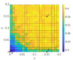
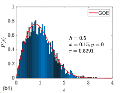
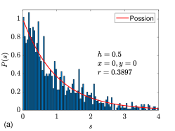
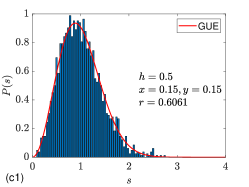
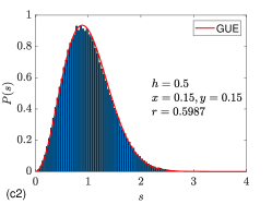
Figure 1: Exact diagonalization results on $r$-value and statistics of energy level spacings for the model on $N=12$ chain (1) with representative parameters. (a) Colour contour plot of $r$-value as functions of ($x,y$) for a given $h_{z}$, obtained from the exact diagonalization of the system with a single set of random number $\left\{x_{j}\right\}$ and $\left\{y_{j}\right\}$ for given ($x,y$). (a, b1, c1) Plots of P(s) for three typical points in $xy$-plane. The results are obtained from a a single set of random number. (b2, c2) Same plots of results obtained from the average over $100$ sets of random number. The Hamiltonian parameters and $r$-value used are indicated in the figure. The color lines indicates Poisson, WD-GOE, and WD-GUE distributions for comparison, the characteristic of integrable and chaotic systems described by random matrix theory. Excellent agreement with the typical distributions is shown, especially for the results from average scheme.

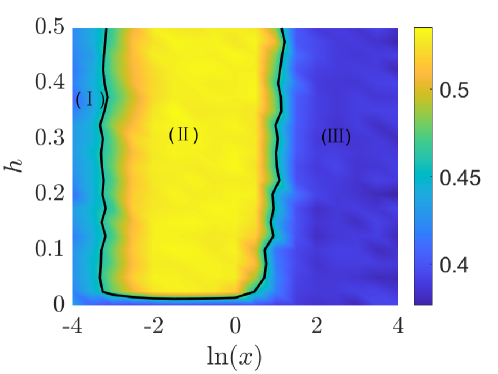
Figure 2: Color contour plot of the average level spacing ratio $r$ as function of $h$ and $x$. There are three regions separated by the black contour line. The distribution of $r(h,x)$ indicates the phase diagram: Region (I) is integrable phase, region (II) is non-integrable phase and region (III) is AL phase. It also indicates that it is always integrable phase in the vicinity of zero $h$. The results are obtained from the average over 10 sets of random number.

According to the above analysis of towers, almost each eigenstate $\left|\psi_{n}(l,m)\right\rangle$ of $H_{0}$ has its own exclusive set of conserved quantum numbers $(n,l,m)$. Thus in the absence of $H_{\mathrm{ran}}$, the system is integrable. In this section, we consider the case with nonzero $x$ and $y$. When the random transverse fields switch on, it spoils all the symmetries related the commutation relations in Eqs (4). In the following, we focus on the questions (i) whether the external field can break the integrability of the system, and (ii) if so, is there towers can prevent the thermalization.

In spite of the absence of exact solutions, this problem can be investigated from numerical simulations, e.g., by examining the probability distribution of the spacings $s$ between energy levels, $P(s)$, which appears to be well described by random matrix theory for whole levels. First of all, the above property of towers yields the following conclusions for two extreme cases: (i) $x=y=0$, but arbitrary $h$; (ii) $x,y\ll\left|h\right|$, where the contributions from $H_{\mathrm{ran}}$ are suppressed sufficiently. In both cases, all the energy levels in each invariant subspace with fixed $m$ are just shifted by amount $mh$. Therefore, the distribution $P(s)$ in each sector indexed by $m$ is Poisson distribution. For the case with nonzero $x$ and $y$, the sectors with different $m$ are hybridized, and then one has to count $P(s)$ for whole levels. In Fig. (1), we plot the energy level spacing statistics of the model with finite $N$. We find that the level spacing distribution is dependent of three parameters $\left(x,y,h\right)$: (i) $\left(x,y,h\right)$ $=\left(0,0,0.5\right)$, $P(s)$ is the Poisson distribution as expected; (ii) $\left(x,y,h\right)$ $=\left(0.15,0,0.5\right)$ or symmetrically $\left(0,0.15,0.5\right)$, $P(s)$ is the Wigner-Dyson from the Gaussian Orthogonal Ensemble (WD-GOE) distribution; (iii) $\left(x,y,h\right)$ $=\left(0.15,0.15,0.5\right)$, $P(s)\$is the Wigner-Dyson from Gaussian Unitary Ensemble (WD-GUE) distribution. Such two distributions is typical of nonintegrable models[30]. The appearence of GOE and GUE distributions accords with the random matrices theory[31], that different types of variables in a random matrix can lead to different distribution forms. If all entries in the Hamiltonian are real and satisfy $H_{ij}=H_{ji}$, the system exhibits the GOE distribution, while the GUE if the entities are complex and satisfy $H_{ij}=H_{ji}^{\ast}$.

Another standard numerical test of integrability is to compute the average level spacing ratio $r$-value[32]. For a selected set of energy levels $\left\{E_{l}\right\}$ (e.g. including the whole levels, or levels in a certain sector), $r$ is the ratio of adjacent gaps as

$$r_{l}=\frac{\mathrm{min}\{s_{l},s_{l+1}\}}{\mathrm{max}\{s_{l},s_{l+1}\}},$$ (19)

and average this ratio over $l$, where $s_{l}$ is level spacings $E_{l}-E_{l-1}$. In general, WD-GOE and WD-GUE distributions correspond to $r\approx 0.53$ and $r\approx 0.60$ respectively, while Poisson distribution is $r\approx 0.39$. We introduce a slightly perturbation in numerical calculations to avoid numerical difficulties arising from degenerate eigenstates, such as superposition of degenerate eigenstates or the occurrence of $0/0$ and so on. In Fig. (2), we also plot a phase in terms of average level spacing ratio $r$ in $h$ vs disorder strength $x$ plane. As can be seen from the figure, there is a crossover from integrable to non-integrable phase, and an emergence of Anderson localization (AL) phase when $x$ is large. There are three regions: (I) and (III) are integrable phases while (II) is non-integrable phase. The strong disorder region (III) is Anderson localization (AL) phase[33]. And now, we concentrate on the non-integrable phase which $x=0.15$. Fig. (3a-c), we plot the $r$-value as functions of ($x,y$) for three types of lattices, which accord to the plots of $P(s)$.

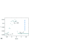
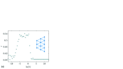
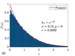
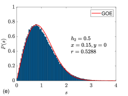
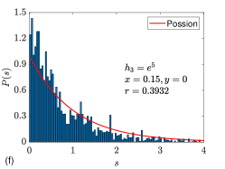
Figure 3: The same plots as Fig. (1) but for three types of clusters with $N=12$. (a-c) Plots of $r$-value as functions of $h_{z}$ for a given ($x,y$), obtained from the exact diagonalization of the system with a single set of random number $\left\{x_{j}\right\}$ and $\left\{y_{j}\right\}$ for given ($x,y$). (d-f) Plots of P(s) for three typical values of $h_{z}$. The results are obtained from the average over $100$ sets of random number. The Hamiltonian parameters and $r$-value used are indicated in the figure. The color lines indicates Poisson and WD-GOE distributions for comparison. Here we only plot the result for the chain, which has no difference with that from other two clusters.

In order to investigate the effect of the uniform field $h$ on the transition of energy level statistics of system with nonzero $x$ and $y$, we plot the $r$-value as function of $h$, and the distributions $P(s)\$at representative points in Fig. (3d-f). We find that the field $h$ takes a subtle role for the integrability of the model. For zero $h$, the nonzero $x$ or $y$ solely cannot induce the non-integrability. On the other hand, so does the large $h$, which is believed to suppress the random field.

4 Quantum scars

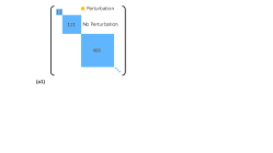
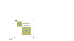
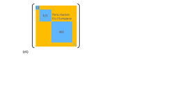
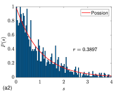
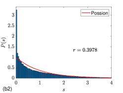
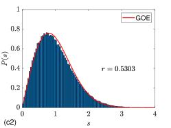
Figure 4: Schematic illustration for structures of the matrices, representing the Hamiltonians with different types of perturbations. (a1) No perturbation with zero $x$ and $y$. The blue blocks represent the matrices in different $l$ sectors, which consist of towers of eigenstates with different $m$. (b1) Switching on the perturbations between towers within each $l$ sector. (c1) Switching on the perturbations between sectors but off perturbations between towers within each $l$ sector. (a2-c2) The corresponding $P(s)$ obtained from the exact diagonalization of the matrices (a1-c1). The plots are obtained from the average over $100$ sets of random number. The parameters and $r$-value used are indicated in the figure. It indicates that the perturbations between towers with different sectors take the crucial role for the transition from integrability to non-integrability of the system.

In this section, we concentrate on the mechanism of the transition from integrability to non-integrability induced by external field and identify the quantum scars. We note that the effects of $H_{\mathrm{ran}}$ on the states $\left\{\left|\psi_{n}(l,m)\right\rangle\right\}$ are two classes: (i) hybridizing the levels with the same $l$, by the nonzero element $\left\langle\psi_{n}(l,m)\right|H_{\mathrm{ran}}\left|\psi_{n^{\prime}}(l,m\pm 1)\right\rangle$; (ii) hybridizing the levels with different $l$, by the nonzero element $\left\langle\psi_{n}(l,m)\right|H_{\mathrm{ran}}\left|\psi_{n^{\prime}}(l^{\prime},m\pm 1)\right\rangle$ with $(l\neq l^{\prime})$. Hence a natural question arises that which types of elements take the role on the transition of the level statistics. To answer this question, we consider two matrices by imposing $\left\langle\psi_{n}(l,m)\right|H_{\mathrm{ran}}\left|\psi_{n^{\prime}}(l,m\pm 1)\right\rangle=0$ and $\left\langle\psi_{n}(l,m)\right|H_{\mathrm{ran}}\left|\psi_{n^{\prime}}(l^{\prime},m\pm 1)\right\rangle=0$, respectively. In Fig. (4) we schematically illustrate the structures of the matrices and plot the corresponding distributions $P(s)$ in comparison to the exact one. It evidently shows that the hybridization between towers with different $l$ is determinant for the transition of the level statistics.

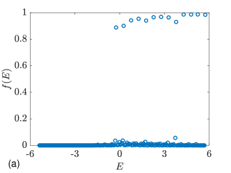
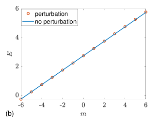
Figure 5: Numerical results obtained by exact diagonalization demonstrating the surviving tower. (a) Plot of $f(E)$ from (20) to reveal the surviving tower by the peaks. (b) Comparison between the locations of the peaks with $E_{1}(N/2,m)$. The parameters are $N=12,x=0.15,y=0,$ and $\Delta=\left(E_{\max}-E_{\min}\right)/200\approx 0.056.$ This indicates that the first tower is immune to the perturbation approximately and then avoids the fast thermalization.

This result indicates that most of the towers are destroyed by the term $H_{\mathrm{ran}}$. Now we consider the question whether there are some towers surviving from the random perturbation. To this end, we perform numerical simulation to investigate the effect of $H_{\mathrm{ran}}$ on the individual tower. In Fig. (5) we plot the perturbed levels in the tower with $l=N/2$. We find that the energy levels are slightly changed, maintaining the equal spacing very well as quantum scar.

In order to measure the fidelity of the quantum scar of the tower $\left|\psi_{n}(l,m)\right\rangle$, we introduce the quantity as function of energy

$$f(E)=\sum_{E-\Delta/2}^{E+\Delta/2}\sum_{m=-l}^{l}\left|\langle\phi(E^{\prime})\left|\psi_{n}(l,m)\right\rangle\right|^{2}$$ (20)

for a set of eigenstates $\left\{\left|\phi(E)\right\rangle\right\}$ of $H$, i.e., $H\left|\phi(E)\right\rangle=E\left|\phi(E)\right\rangle$. Here we take small $\Delta$ to select the quasi-degenerate states near the tower energy levels. Obviously, for perfect quantum scar, where $\left\{\left|\phi(E)\right\rangle\right\}$ contains $\left\{\left|\psi_{n}(l,m)\right\rangle\right\}$, we should have

$$f(E)=\sum_{E-\Delta/2}^{E+\Delta/2}\sum_{m=-l}^{l}\delta\left[E^{\prime}-E_{n}(l,m)\right],$$ (21)

i,e., $f(E)=1$ when $E=E_{n}(l,m)$. In the presence of nonzero $H_{\mathrm{ran}}$, the peaks of $f(E)$ indicate and measure the efficiency of the surviving towers for a given perturbed $H$. Numerical simulation is performed for the tower $\left|\psi_{1}(6,m)\right\rangle$ as an example. Based on the results of exact diagonalization, $2\times 6+1$ peaks of $f(E)$ is obtained and their positions correspond to the energy levels of the surviving tower. In Fig. (5), we plot $f(E)$ and its peaks to compare the energy ladder for finite system to demonstrate the surviving tower. We find that the peaks of $f(E)$ approach to $1$ for high energy levels and are more than $0.83$ for the rest. The energy levels of the surviving tower have a slight deviation from the exact ladder. The results indicate that the surviving tower is immune to the perturbation approximately and then avoids the fast thermalization. The behavior of $f(E)$ in this example can be used to explain the dynamics for the specific initial states in the following section. Here we only present the $f(E)$ for the chain system for the sake of concise presentation. In fact, similar numerical results are obtained for other two types of clusters.

5 Revival of W and GHZ states

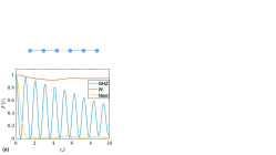
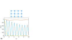
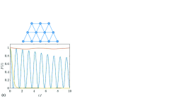
Figure 6: Plots of the fidelity from (25) for three types of Heisenberg clusters. The initial states are W state $\left|\mathrm{W}\right\rangle=\left|\psi_{1}(6,5)\right\rangle$, GHZ state $\left|\mathrm{GHZ}\right\rangle$ $=\frac{1}{\sqrt{2}}\left(\left|\psi_{1}(6,6)\right\rangle+\left|\psi_{1}(6,-6)\right\rangle\right)$, and Neel state $\left|\mathrm{Neel}\right\rangle=\left|\uparrow\downarrow\uparrow\downarrow\uparrow\downarrow\uparrow\downarrow\uparrow\downarrow\uparrow\downarrow\right\rangle$. The parameters are $N=12$, $x=0.15$, $y=0$, and $h=0.5$. We find that the behaviors of the fidelity are almost independent of the geometry of the clusters. Analyses and discussions are given in the text.

So far we have shown that the external field can induce the thermalization for an isotropic clusters. In addition, such systems host special nonthermal eigenstates that should support periodic revival. Inspired by recent experiments with Rydberg atoms, where nonthermal periodic revival dynamics has been observed for initial Neel state[34, 35], we will examine the dynamics for three states. They are W state $\left|\mathrm{W}\right\rangle=\frac{1}{\sqrt{N}}Q\left|\Uparrow\right\rangle$, GHZ state $\left|\mathrm{GHZ}\right\rangle=\frac{1}{\sqrt{2}}\left(\left|\Uparrow\right\rangle+\left|\Downarrow\right\rangle\right)$ and Neel state, which can be expressed in the form

$$\left|\mathrm{W}\right\rangle=\left|\psi_{1}(N/2,N/2-1)\right\rangle$$ (22)

and

$$\left|\mathrm{GHZ}\right\rangle=\frac{1}{\sqrt{2}}\left(\left|\psi_{1}(N/2,N/2)\right\rangle+\left|\psi_{1}(N/2,-N/2)\right\rangle\right),$$ (23)

and

$$\left|\mathrm{Neel}\right\rangle=\left|\uparrow\downarrow\uparrow\downarrow...\uparrow\downarrow\right\rangle,$$ (24)

respectively. Here states $\left|\mathrm{W}\right\rangle$ and $\left|\mathrm{GHZ}\right\rangle$ are two different typical multipartite entangled states, which are usually referred to as maximal entanglement[36]. The two states are included in the tower with $l=N/2$, while the Neel state $\left|\mathrm{Neel}\right\rangle$ is not. In practice for quantum computing, an initial state made of many-body scar states repeatedly returns to itself in time evolution, preventing the loss of quantum information through thermalization. To demonstrate this point, we compute the time evolution for the initial states $\left|\psi(0)\right\rangle=\left|\mathrm{GHZ}\right\rangle$, $\left|\mathrm{W}\right\rangle$ and $\left|\mathrm{Neel}\right\rangle$, under the Heisenberg clusters with finite $N$. We introduce the fidelity

$$F(t)=\left|\left\langle\psi(0)\right|e^{-iHt}\left|\psi(0)\right\rangle\right|^{2},$$ (25)

to measure the feature of revival. As can be seen in Fig. (6), the quantity $F(t)$ shows the periodic revivals for W and GHZ states, but relatively fast decay for initial Neel state. From the profile of $f(E)$ in Fig. (5a), the behaviors of $F(t)$ in Fig. (6) for three initial states can be explained as following. (i) The $\left|\mathrm{W}\right\rangle$ state is almost the eigenstate of $H$ since the second peak of $f(E)$ is very close to $1$. It results in $F(t)\approx 1$ for the time evolution as expected. (ii) The $\left|\mathrm{GHZ}\right\rangle$ state is related first and the last peaks of $f(E)$. We note that the last peak of $f(E)\approx 0.83$. This deviation from $1$ definitely leads to a light dumping oscillation. (iii) As for the Neel state $\left|\mathrm{Neel}\right\rangle$, it is a component of $\left|\psi_{1}(6,0)\right\rangle$ with a very small amplitude

$$\langle\psi_{1}(6,0)\left|\mathrm{Neel}\right\rangle=\sqrt{\frac{1}{C_{12}^{6}}}\approx 0.033.$$ (26)

Although it is related to the middle peak of $f(E)$, it is almost out of the scar. Then the $F(t)$ of Neel state decays fast. The above analysis is based on the result of $f(E)$ for the chain system. However, the same conclusion can be obtained for other types of clusters. As expected, numerical simulations show that the behavior of $F(t)$ is almost independent of the geometry of the clusters. In addition, we would like to point out that, for another W state $\left|\mathrm{W}^{\prime}\right\rangle=\frac{1}{\sqrt{N}}Q^{{\dagger}}\left|\Downarrow\right\rangle$, the fidelity should be not so perfect as that of $\left|\mathrm{W}^{\prime}\right\rangle$ due to the shrinkage of the last second peak of $f(E)$. We would like to point out that the profile of $f(E)$ is sensitive to a very small $\Delta$, and the results presented in Fig. (5) and (6) are selected from the cases with a finite number of sets of random numbers. It is unavoidable one may get a very different result by accident. We emphasize again that the conclusions obtained here hold only to small size systems, i.e., it is not sure whether or not the random field we applied can result in localization for large $N$ system, preventing the thermalization.

In addition, we also employ the entanglement spectrum (ES) to support the existence of quantum scars. The ES has been used to study quantum scars and distinguish MBL systems from ergodic systems recently[37, 38, 39]. It represents the eigenvalues $\left\{E_{n}\right\}$ of the reduced density matrix,

$$\rho_{s}=\sum\limits_{n}E_{n}\left|n\right\rangle_{s}\left\langle n\right|_{s},$$ (27)

which is obtained from the Schmidt decomposition of $\left|\psi\right\rangle=\sum\limits_{n}\sqrt{E_{n}}\left|n\right\rangle_{s}\otimes\left|n\right\rangle_{\bar{s}}$. For quantum scars, the ES will exhibit a large gap. Therefore, we plotted the ES for GHZ, W, and Neel states in Fig. (7a). Here we divide the entire system into two equally sized parts to compute the reduced density matrix. And we found that the ES of GHZ and W states have a significant gap for sufficiently long time ($t=500$), while the Neel state does not. This is also evidence that they are quantum scars. On the other hand, recent studies have found that fidelity out-of-time-order correlator (FOTOC) exhibits a non-stable dynamical behavior with respect to quantum scars[40]. However in our case, the FOTOC, which is defined as $f_{is}=\sum\limits_{\alpha=x,y,z}\left(\left\langle s_{i\alpha}^{2}\right\rangle-\left\langle s_{i\alpha}\right\rangle^{2}\right)/s^{2}$, for the initial W and GHZ states do not exhibit oscillation behavior. It may be due to the fact that the W and GHZ states are the quasi-eigenstate and maximally entangled state, respectively.

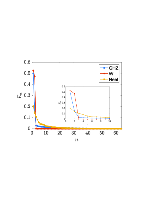
Figure 7: Entanglement spectrum (ES) of GHZ, W and Neel states under long-time evolution ($t=500$) in the regions of non-integrable ($h=0.5$ and $x=0.15$). In the inset, the large vision of front part of spectrum. The gaps for GHZ and W states are evident.

6 Conclusions

We have demonstrated that the external fields, can induce dramatic transition from integrability to non-integrability for different clusters of isotropic Heisenberg model. Numerical results show that the cooperation between the uniform field one direction, and the random field in other two directions, takes the crucial role for such a transition. While generic initial states are expected to thermalize, we show that there is a tower of eigenstates leads to weak ergodicity breaking in the form of equal level spacing approximately. Specifically, this quantum many-body scar covers two important states, W and GHZ states. The obtained results indicate that the random field with moderate strength can induce non-integrability for finite size clusters. This finding reveals the possibility of quantum information processing that is immune to the thermalization in finite size quantum spin clusters at nonzero temperature.

References

References

- [1] Shiraishi N and Mori T 2017 Phys. Rev. Lett. 119 030601
- [2] Moudgalya S, Rachel S, Bernevig B A and Regnault N 2018 Phys. Rev. B 98 235155
- [3] Moudgalya S, Regnault N and Bernevig B A 2018 Phys. Rev. B 98, 235156
- [4] Khemani V, Laumann C R and Chandran A 2019 Phys. Rev. B 99 161101(R)
- [5] Ho W W, Choi S, Pichler H and Lukin M D 2019 Phys. Rev. Lett. 122 040603
- [6] Shibata N, Yoshioka N and Katsura H 2020 Phys. Rev. Lett. 124 180604
- [7] McClarty P A, Haque M, Sen A and Richter J 2020 Phys. Rev. B 102 224303
- [8] Richter J and Pal A 2022 Phys. Rev. Research 4 L012003
- [9] Jeyaretnam J, Richter J and Pal A 2021 Phys. Rev. B 104 014424
- [10] Turner C J, Michailidis A A, Abanin D A, Serbyn M and Z. Papic 2018 Nat. Phys. 14 745
- [11] Turner C J, Michailidis A A, Abanin D A, Serbyn M and Papic Z 2018 Phys. Rev. B 98 155134
- [12] Shiraishi N 2019 J. Stat. Mech. 083103
- [13] Lin C-J and Motrunich O I 2019 Phys. Rev. Lett. 122 173401
- [14] Choi S, Turner C J, Pichler H, Ho W W, Michailidis A A, Papić Z, Serbyn M, Lukin M D and Abanin D A 2019 Phys. Rev. Lett. 122 220603
- [15] Khemani V, Hermele M and Nandkishore R 2020 Phys. Rev. B 101 174204
- [16] Dooley S and Kells G 2020 Phys. Rev. B 102 195114
- [17] Dooley S 2021 PRX Quantum 2 020330
- [18] Fukuhara T et al. 2013 Nat. Phys. 9 235
- [19] Fukuhara T et al. 2013 Nature (London) 502 76
- [20] Ronzheimer J P, Schreiber M, Braun S, Hodgman S S, Langer S, McCulloch I P, Heidrich-Meisner F, Bloch I and Schneider U 2013 Phys. Rev. Lett. 110 205301
- [21] Schneider U, Hackermüller L et al. 2012 Nat. Phys. 8 213
- [22] Cheneau M et al. 2012 Nature (London) 481 484
- [23] Jurcevic P et al. 2014 ibid. 511 202
- [24] Anderson P W 1958 Phys. Rev. 109 1492
- [25] Znidaric M, Prosen T and Prelovsek P 2008 Phys. Rev. B 77 064426
- [26] Pal A and Huse D A 2010 Phys. Rev. B 82 174411
- [27] Vosk R and Altman E 2013 Phys. Rev. Lett. 110 067204
- [28] Huse D A, Nandkishore R, Oganesyan V, Pal A and Sondhi S L 2013 Phys. Rev. B 88 014206
- [29] Schecter M and Iadecola T 2019 Phys. Rev. Lett. 123, 147201
- [30] Oliviero S F E, Leone L, Caravelli F and Hamma A 2021 SciPost Phys. 10 076
- [31] D’Alessio L, Kafri Y, Polkovnikov A and Rigol M 2016 Advances in Physics 65 (3) 239–362.
- [32] Oganesyan V and Huse D A 2007 Phys. Rev. B 75 155111
- [33] We obtained this conclusion based on the numerical simulation of the out-of-time-order correlators (OTOC) [42, 41] for our system in the region (III).
- [34] Bernien H, Schwartz S, Keesling A, Levine H, Omran A, Pichler H, Choi S, Zibrov A S, Endres M, Greiner M, Vuletic V and Lukin M D 2017 Nature (London) 551 579
- [35] Bluvstein D, Omran A, Levine H, Keesling A, Semeghini G, Ebadi S, Wang T T, Michailidis A A, Maskara N, Ho W W, Choi S, Serbyn M, Greiner M, Vuletic V and Lukin M D 2021 Science 371 1355
- [36] Migdał P, Rodriguez-Laguna J, Lewenstein M 2013 Phys. Rev. A 88 (1) 012335
- [37] Mondal D, Sinha S, Ray S, Kroha J and Sinha S 2022 Phys. Rev. A 106 043321
- [38] Yang Z-C, Chamon C, Hamma A and Mucciolo E R 2015 Phys. Rev. Lett. 115 267206
- [39] Serbyn M, Michailidis A A, Abanin D A and Papić Z 2016 Phys. Rev. Lett. 117 160601
- [40] Mondal D, Sinha S and Sinha S 2022 Phys. Rev. E 105, 014130
- [41] Fan R, Zhang P, Shen H and Zhai H 2017 Sci. Bull. 62 707–711
- [42] Li J, Fan R, Wang H, Ye B, Zeng B, Zhai H, Peng X and Du J 2017 Phys. Rev. X 7 031011