Influence of Different Subgrid Scale Models in Low-Order LES of Supersonic Jet Flows

Abstract

The present work is concerned with a study of large eddy simulations (LES) of unsteady turbulent jet flows. In particular, the present analysis is focused on the effects of the subgrid scale modeling used when a second-order spatial discretization methodology is employed for the numerical simulations. The present effort addresses perfectly expanded supersonic jets, because the authors want to emphasize the effects of the jet mixing phenomena. The LES formulation is discretized using the finite difference approach, after the equations are rewritten in a generalized coordinate system. Both space and time discretizations are second order accurate, and an explicit time march is adopted. Special care is dedicated to the discretization of the energy equation in order to appropriately model the energy equation of the filtered Navier-Stokes formulation. The classical Smagorinsky, the dynamic Smagorinsky and the Vreman models are the subgrid scale closures selected for the present work. The computational results are compared to data in the literature in order to validate the present simulation tool. Results indicate that the characteristics of numerical discretization can overcome effects of the subgrid scale models. A detailed analysis is presented for the performance of each subgrid closure in the numerical context here considered.

1 Introduction

A novel compressible large eddy simulation (LES) tool has recently been developed at Instituto de Aeronáutica e Espaço (IAE) Junqueira-Junior et al. [2015]. This numerical tool was developed, to a large extent, to generate unsteady flow data on large launch vehicle propulsion exhaust jets, for which the noise generated on certain flight conditions can be extremely relevant for dimensioning of payload structures being carried by the launcher. The approach intended was to study the aeroacoustics of such jets using a hybrid approach, based on the Ffowcs Williams and Hawkings analogy Wolf et al. [2012]. As such, and considering previous capabilities available in the research group Bigarella [2002, 2007], the decision was to use a low order spatial discretization approach for such development. The LES tool developed was denoted JAZzY, and further details of its formulation and computational performance can be found in Refs. Junqueira-Junior [2016], Junqueira-Junior et al. [2015].

It should be emphasized that the use of low order spatial discretization for LES calculations is not a new idea, and it is actually suggested by several recognized research groups in the world, as indicated, for instance, in Ref. Choi and Moin [2012]. The main aspect involved in such proposition is computational efficiency, which can typically be achieved with the low order spatial discretization. However, the critical question that arises in such context is the effectiveness of the subgrid scale modeling Li and Wang [2015], Wang [2015]. Therefore, the present paper is precisely directed towards the study of the effects of the subgrid scale modeling used when a second-order spatial discretization methodology is employed for the numerical simulations with an LES formulation. The subgrid scale closures included in the present study are the classical Smagorinsky model Lilly [1965, 1967], Smagorinsky [1963], the dynamic Smagorinsky model Germano et al. [1991], Moin et al. [1991] and the Vreman model Vreman [2004].

In the present effort, the LES formulation is discretized using the finite difference approach, after the governing equations are rewritten in general curvilinear coordinates Junqueira-Junior [2016], Junqueira-Junior et al. [2015]. Inviscid and viscous numerical fluxes are calculated using a second-order accurate centered scheme with the explicit addition of artificial dissipation terms. Time march uses a five-stage, second-order accurate, explicit Runge-Kutta scheme. The present formulation for the energy equation is based on the System I set of equations Vreman [1995], in order to appropriately model the filtered terms of the energy equation. The test cases address numerical simulations of perfectly expanded jet flows, and the current results are compared to both numerical Mendez et al. [2010] and experimental Bridges and Wernet [2008] independent data.

2 Large Eddy Simulation Filtering

The large eddy simulation is based on the principle of scale separation, which is addressed as a filtering procedure in a mathematical formalism. A modified version of the the System I filtering approach Vreman [1995] is used in present work, which is given by

$$\begin{array}[]{c}\displaystyle\frac{\partial\overline{\rho}}{\partial t}+\frac{\partial}{\partial x_{j}}\left(\overline{\rho}\widetilde{u_{j}}\right)=0\,\mbox{,}\\ \displaystyle\frac{\partial}{\partial t}\left(\overline{\rho}\widetilde{u_{i}}\right)+\frac{\partial}{\partial x_{j}}\left(\overline{\rho}\widetilde{u_{i}}\widetilde{u_{j}}\right)+\frac{\partial\overline{p}}{\partial x_{i}}-\frac{\partial{\tau}_{ij}}{\partial x_{j}}+\frac{1}{3}\frac{\partial}{\partial x_{j}}\left({\delta}_{ij}\sigma_{kk}\right)=0\,\mbox{,}\\ \displaystyle\frac{\partial\overline{e}}{\partial t}+\frac{\partial}{\partial x_{j}}\left[\left(\overline{e}+\overline{p}\right)\widetilde{u_{j}}\right]-\frac{\partial}{\partial x_{j}}\left({\tau}_{ij}\widetilde{u_{i}}\right)+\frac{1}{3}\frac{\partial}{\partial x_{j}}\left[\left(\delta_{ij}{\sigma}_{kk}\right)\widetilde{u_{i}}\right]+\frac{\partial{q}_{j}}{\partial x_{j}}=0\,\mbox{,}\end{array}$$ (1)

in which $t$ and $x_{i}$ are independent variables representing time and spatial coordinates of a Cartesian coordinate system, x, respectively. The components of the velocity vector, u, are written as $u_{i}$ and $i=1,2,3$. Density, pressure and total energy per unit volume are denoted by $\rho$, $p$ and $e$, respectively. The $\left(\overline{\cdot}\right)$ and $\left(\tilde{\cdot}\right)$ operators are used in order to represent filtered and Favre averaged properties, respectively. The System I formulation neglects the double correlation term and the total energy per unit volume is written as

$$\overline{e}=\frac{\overline{p}}{\gamma-1}+\frac{1}{2}\rho\widetilde{u}_{i}\widetilde{u}_{i}\,\mbox{.}$$ (2)

The heat flux, $q_{j}$, is given by

$${q}_{j}=\left(\kappa+{\kappa}_{sgs}\right)\frac{\partial\widetilde{T}}{\partial x_{j}}\,\mbox{.}$$ (3)

where $T$ is the static temperature and $\kappa$ is the thermal conductivity coefficient, which can by expressed as

$$\kappa=\frac{\mu C_{p}}{Pr}\,\mbox{,}$$ (4)

The thermal conductivity coefficient is a function of the specific heat at constant pressure, $Cp$, of the Prandtl number, $Pr$, which is equal to $0.72$ for air, and of the dynamic viscosity coefficient, $\mu$. The SGS thermal conductivity coefficient, $\kappa_{sgs}$, is written as

$$\kappa_{sgs}=\frac{\mu_{sgs}C_{p}}{{Pr}_{sgs}}\,\mbox{,}$$ (5)

where ${Pr}_{sgs}$ is the SGS Prandtl number, which is equal to $0.9$ for static SGS models and $\mu_{sgs}$ is the eddy viscosity coefficient which is calculated by the SGS closure. The dynamic viscosity coefficient, $\mu$, can be calculated using the Sutherland Law,

$$\mu\left(\widetilde{T}\right)=\mu_{\infty}\left(\frac{\widetilde{T}}{\widetilde{T}_{\infty}}\right)^{\frac{3}{2}}\frac{\widetilde{T}_{0}+S_{1}}{\widetilde{T}+S_{1}}\mbox{ , } \mbox{with}\>S_{1}=110.4K\,\mbox{.}$$ (6)

Density, static pressure and static temperature are correlated by the equation of state, given by

$$\overline{p}={\overline{\rho}}R\widetilde{T}\,\mbox{,}$$ (7)

where $R$ is the gas constant, written as

$$R=C_{p}-C_{v}\,\mbox{,}$$ (8)

and $C_{v}$ is the specif heat at constant volume. The shear-stress tensor, $\tau_{ij}$, is written according to the Stokes hypothesis and includes the eddy viscosity coefficient, $\mu_{sgs}$,

$${\tau}_{ij}=2\left(\mu+{\mu}_{sgs}\right)\left(\tilde{S}_{ij}-\frac{1}{3}\delta_{ij}\tilde{S}_{kk}\right)\,$$ (9)

in which the components of the rate-of-strain tensor, $\tilde{S}_{ij}$, are given by

$$\tilde{S}_{ij}=\frac{1}{2}\left(\frac{\partial\tilde{u}_{i}}{\partial x_{j}}+\frac{\partial\tilde{u}_{j}}{\partial x_{i}}\right)\,\mbox{.}$$ (10)

The SGS stress tensor components are written using the eddy viscosity coefficient Sagaut [2002],

$$\sigma_{ij}=-2\mu_{sgs}\left(\tilde{S}_{ij}-\frac{1}{3}\tilde{S}_{kk}\right)+\frac{1}{3}\delta_{ij}\sigma_{kk}\,\mbox{.}$$ (11)

The eddy viscosity coefficient, $\mu_{sgs}$, and the components of the isotropic part of the SGS stress tensor, $\sigma_{kk}$, are modeled by the SGS closure.

3 Subgrid Scale Modeling

The present section is directed towards the description of the turbulence modeling and the theoretical formulation of subgrid scale closures included in the present work. The closure models presented here are based on the homogeneous turbulence theory, which is usually developed in the spectral space as an attempt to quantify the interaction between the different scales of turbulence.

3.1 Smagorinsky Model

The Smagorinsky model Smagorinsky [1963] is one of the simplest algebraic models for the deviatoric part of the SGS tensor used in large eddy simulations. The isotropic part of the SGS tensor is neglected for the Smagorinsky model in the current work. This SGS closure is a classical model based on the large scale properties and it is written as

$${\mu_{sgs}=\overline{\rho}\,\left(C_{s}\Delta\right)^{2}|\widetilde{S}|\,\mbox{,}}$$ (12)

where

$$|\tilde{S}|=\left(2\tilde{S}_{ij}\tilde{S}_{ij}\right)^{\frac{1}{2}}\,\mbox{,}$$ (13)

$\Delta$ is the filter size and $C_{s}$ is the Smagorinsky constant. Several attempts can be found in the literature regarding the evaluation of the Smagorinsky constant. The value of this constant is adjusted to improve the results for different flow configurations. In practical terms, the Smagorinsky subgrid model has a flow dependency on the constant, which takes values ranging from $0.1$ to $0.2$ depending on the flow. The value suggested by Lilly Lilly [1967], $C_{s}=0.148$, is used in the current work.

This model is generally over dissipative in regions of large mean strain. This is particularly true in the transitional region between laminar and turbulent flows. Moreover, the limiting behavior near the wall is not correct, and the model predictions correlate poorly with the exact subgrid scale tensor Garnier et al. [2009]. However, it is a very simple model and, with the use of damping functions and good calibration, it can be successfully applied in large eddy simulations.

3.2 Vreman Model

Vreman Vreman [2004] proposed a turbulence model that can correctly predict inhomogeneous turbulent flows. For such flows, the eddy viscosity should become small in laminar and transitional regions. This requirement is unfortunately not satisfied by existing simple eddy viscosity closures such as the classic Smagorinsky model Deardorff [1970], Lilly [1965], Smagorinsky [1963]. The Vreman SGS model is also very simple and it is given by

$${\mu_{sgs}=\overline{\rho}\,\bm{c}\,\sqrt{\frac{B_{\beta}}{\alpha_{ij}\alpha_{ij}}}\,\mbox{ ,}}$$ (14)

with

$$\alpha_{ij}=\frac{\partial\tilde{u}_{j}}{\partial x_{i}}\,\mbox{ ,}$$ (15)

$${B_{\beta}=\beta_{11}\beta_{22}-\beta_{12}^{2}+\beta_{11}\beta_{33}-\beta_{13}^{2}+\beta_{22}\beta_{33}-\beta_{23}^{2}\,\mbox{ ,}}$$ (16)

and

$${\beta_{ij}=\Delta^{2}_{m}\alpha_{mi}\alpha_{mj}}\mbox{ .}$$ (17)

The $\bm{c}$ constant is related to the Smagorinsky constant, $C_{s}$, and it is given by

$$\bm{c}=2.5\,C_{s}^{2}\,\mbox{,}$$ (18)

and $\Delta_{m}$ is the filter width in each direction. In the present work, the isotropic part of the SGS tensor is neglected for the Vreman model. The $\alpha$ symbol represents the matrix of first order derivatives of the filtered components of velocity, $\tilde{u}_{i}$. The SGS eddy viscosity coefficient is defined as zero when $\alpha_{ij}\alpha_{ij}$ equals zero. Vreman Vreman [2004] states that the $\beta_{ij}$ tensor is proportional to the Clark model Clark et al. [1979], Leonard [1974] in its general anisotropic form Vreman et al. [1996].

The Vreman model can be classified as a very simple model because it is expressed in first-order derivatives and it does not involves explicit filtering, averaging and clipping procedures, and it is rotationally invariant for isotropic filter widths. The model was originally created for incompressible flows and it has presented good results for two incompressible flows configurations: the transitional and turbulent mixing layer at high Reynolds number and the turbulent channel flow Vreman et al. [1996]. In both cases, the Vreman model is found to be more accurate than the classical Smagorinsky model and as good as the dynamic Smagorinsky model.

3.3 Dynamic Smagorinsky Model

Germano et al. Germano [1990] developed a dynamic SGS model in order to overcome the issues of the classical Smagorinsky closure. The model uses the strain rate fields at two different scales and, thus, extracts spectral information in the large scale field to extrapolate the small stresses Moin et al. [1991]. The coefficients of the model are computed instantaneously in the dynamic model. They are a function of the positioning in space and time rather than being specified a priori. Moin et al. Moin et al. [1991] extended the work of Germano for compressible flows. The dynamic Smagorinsky model for compressible flow configurations is detailed in the present section.

The dynamic model introduces the test filter, $\widehat{\left(\cdot\right)}$, which has a larger filter width, $\widehat{\Delta}$, than the one of the resolved grid filter, $\overline{\left(\cdot\right)}$. The use of test filters generates a second field with larger scales than the resolved field. The Yoshizawa model Yoshizawa [1986] is used for the isotropic portion of the SGS tensor and it is written as

$$\sigma_{ll}=2C_{I}\overline{\rho}{\Delta}^{2}|\tilde{S}|^{2}\,\mbox{,}$$ (19)

where $C_{I}$ is defined by

$$C_{I}=\frac{\biggl{\langle}\widehat{\overline{\rho}\tilde{u}_{l}\tilde{u}_{l}}-\left(\widehat{\overline{\rho}\tilde{u}_{l}}\widehat{\overline{\rho}\tilde{u}_{l}}/\widehat{\overline{\rho}}\right)\biggr{\rangle}}{\biggl{\langle}2\widehat{\Delta}^{2}\widehat{\overline{\rho}}|\widehat{\overline{S}}|^{2}-2{\Delta}^{2}\widehat{\overline{\rho}|\overline{S}|^{2}}\biggr{\rangle}}\,\mbox{.}$$ (20)

A volume averaging, here indicated by $\langle\,\,\rangle$, is suggested by Moin et al Moin et al. [1991] and by Garnier et al Garnier et al. [2009] in order to avoid numerical issues. The eddy viscosity, $\mu_{sgs}$, is calculated using the same approach used by static Smagorinsky model,

$$\mu_{sgs}=\left(\rho C_{ds}\Delta\right)^{2}|\tilde{S}|\,\mbox{,}$$ (21)

where

$$|\tilde{S}|=\left(2\tilde{S}_{ij}\tilde{S}_{ij}\right)^{\frac{1}{2}}\,\mbox{,}$$ (22)

and $C_{ds}$ is the dynamic constant of the model, which is given by

$$C_{ds}=\frac{\biggl{\langle}\left[\widehat{\overline{\rho}\tilde{u}_{i}\tilde{u}_{j}}-\left(\widehat{\overline{\rho}\tilde{u}_{i}}\widehat{\overline{\rho}\tilde{u}_{j}}/\widehat{\overline{\rho}}\right)\right]\tilde{S}_{ij}-\frac{1}{3}\tilde{S}_{mm}\left(\mathscr{T}_{ll}-\widehat{\sigma}_{ll}\right)\biggr{\rangle}}{\biggl{\langle}2{\Delta}^{2}\left[\widehat{\overline{\rho}|\tilde{S}|\tilde{S}_{ij}}\tilde{S}_{ij}-\frac{1}{3}\left(\overline{\rho}|\tilde{S}|\tilde{S}_{mm}\right)^{\widehat{}}\tilde{S}_{ll}\right]-2\widehat{\Delta}^{2}\left(\widehat{\overline{\rho}}|\widehat{\tilde{S}}|\widehat{\tilde{S}}_{ij}\tilde{S}_{ij}-\frac{1}{3}\widehat{\overline{\rho}}|\widehat{\tilde{S}}|\widehat{\tilde{S}}_{mm}\tilde{S}_{ll}\right)\biggr{\rangle}}\,\mbox{.}$$ (23)

The SGS Prandtl number is computed using the dynamic constant, $C_{ds}$, and written as

$${Pr}_{sgs}=C_{ds}\frac{\biggl{\langle}\Delta^{2}\biggl{(}\overline{\rho}|\tilde{S}|\frac{\partial\overset{\sim}{T}}{\partial x_{j}}\biggr{)}^{\widehat{}}\,\frac{\partial\overset{\sim}{T}}{\partial x_{j}}-\widehat{\Delta}^{2}\widehat{\overline{\rho}}|\widehat{\tilde{S}}|\frac{\partial\overset{\sim}{T}}{\partial x_{j}}\frac{\partial\overset{\sim}{T}}{\partial x_{j}}\biggr{\rangle}}{\biggl{\langle}\left[\widehat{\overline{\rho}\tilde{u}_{j}\overset{\sim}{T}}-\left(\widehat{\overline{\rho}\tilde{u_{j}}}\widehat{\overline{\rho}\overset{\sim}{T}}\right)/\widehat{\overline{\rho}}\right]\frac{\partial\overset{\sim}{T}}{\partial x_{j}}\biggr{\rangle}}\,\mbox{.}$$ (24)

4 Transformation of Coordinates

In the present work, the filtered Navier-Stokes equations are written in strong conservation law form for a 3-D general curvilinear coordinate system as

$$\frac{\partial\hat{Q}}{\partial t}+\frac{\partial}{\partial\xi}\left(\hat{\mathbf{E}}_{e}-\hat{\mathbf{E}}_{v}\right)+\frac{\partial}{\partial\eta}\left(\hat{\mathbf{F}}_{e}-\hat{\mathbf{F}}_{v}\right)+\frac{\partial}{\partial\zeta}\left(\hat{\mathbf{G}}_{e}-\hat{\mathbf{G}}_{v}\right)=0\,\mbox{.}$$ (25)

The general coordinate transformation adopted in the present case can be written as

$$\xi = \xi{\left(x,y,z\right)}\,\mbox{,}$$

$$\eta = \eta{\left(x,y,z\right)}\,\mbox{,}$$ (26)

$$\zeta = \zeta{\left(x,y,z\right)}\ \,\mbox{.}$$

For the simulations performed in the present paper, $\xi$ is the axial jet flow direction, $\eta$ is the radial direction and $\zeta$ is the azimuthal direction. The new vector of conserved properties in general curvilinear coordinates can be written as

$$\hat{Q}=J^{-1}\left[\overline{\rho}\quad\overline{\rho}\tilde{u}\quad\overline{\rho}\tilde{v}\quad\overline{\rho}\tilde{w}\quad\overline{e}\right]^{T}\quad\mbox{ .}$$ (27)

Here, $J$ is the Jacobian of the transformation, which could be expressed as

$$J=\left(x_{\xi}y_{\eta}z_{\zeta}+x_{\eta}y_{\zeta}z_{\xi}+x_{\zeta}y_{\xi}z_{\eta}-x_{\xi}y_{\zeta}z_{\eta}-x_{\eta}y_{\xi}z_{\zeta}-x_{\zeta}y_{\eta}z_{\xi}\right)^{-1}\,\mbox{ .}$$ (28)

The inverse metric terms of the transformation, which are used to compute the transformation Jacobian, can be directly computed by central finite differences from the mesh information. Such computation is given by

$$\displaystyle{x_{\xi}=\frac{\partial x}{\partial\xi}\,\mbox{,}} \displaystyle{x_{\eta}=\frac{\partial x}{\partial\eta}\,\mbox{,}} \displaystyle{x_{\zeta}=\frac{\partial x}{\partial\zeta}\,\mbox{,}}$$

$$\displaystyle{y_{\xi}=\frac{\partial y}{\partial\xi}\,\mbox{,}} \displaystyle{y_{\eta}=\frac{\partial y}{\partial\eta}\,\mbox{,}} \displaystyle{y_{\zeta}=\frac{\partial y}{\partial\zeta}\,\mbox{,}}$$ (29)

$$\displaystyle{z_{\xi}=\frac{\partial z}{\partial\xi}\,\mbox{,}} \displaystyle{z_{\eta}=\frac{\partial z}{\partial\eta}\,\mbox{,}} \displaystyle{z_{\zeta}=\frac{\partial z}{\partial\zeta}\,\mbox{.}}$$

The inviscid flux vectors in general curvilinear coordinates, $\hat{\mathbf{E}}_{e}$, $\hat{\mathbf{F}}_{e}$ and $\hat{\mathbf{G}}_{e}$, can be written as

$$\hat{\mathbf{E}}_{e}=J^{-1}\left\{\begin{array}[]{c}\overline{\rho}U\\ \overline{\rho}\tilde{u}U+\overline{p}\xi_{x}\\ \overline{\rho}\tilde{v}U+\overline{p}\xi_{y}\\ \overline{\rho}\tilde{w}U+\overline{p}\xi_{z}\\ \left(\overline{e}+\overline{p}\right)U\end{array}\right\}\,\mbox{ ,} \hat{\mathbf{F}}_{e}=J^{-1}\left\{\begin{array}[]{c}\overline{\rho}V\\ \overline{\rho}\tilde{u}V+\overline{p}\eta_{x}\\ \overline{\rho}\tilde{v}V+\overline{p}\eta_{y}\\ \overline{\rho}\tilde{w}V+\overline{p}\eta_{z}\\ \left(\overline{e}+\overline{p}\right)V\end{array}\right\}\,\mbox{ ,}$$ (40)

$$\hat{\mathbf{G}}_{e}=J^{-1}\left\{\begin{array}[]{c}\overline{\rho}W\\ \overline{\rho}\tilde{u}W+\overline{p}\zeta_{x}\\ \overline{\rho}\tilde{v}W+\overline{p}\zeta_{y}\\ \overline{\rho}\tilde{w}W+\overline{p}\zeta_{z}\\ \left(\overline{e}+\overline{p}\right)W\end{array}\right\}\,\mbox{.}$$ (46)

The contravariant velocity components, $U$, $V$ and $W$, are calculated as

$${U=\xi_{x}\overline{u}+\xi_{y}\overline{v}+\xi_{z}\overline{w}\,\mbox{,}}$$

$${V=\eta_{x}\overline{u}+\eta_{y}\overline{v}+\eta_{z}\overline{w}\,\mbox{,}}$$ (47)

$${W=\zeta_{x}\overline{u}+\zeta_{y}\overline{v}+\zeta_{z}\overline{w}\,\mbox{.}}$$

The metric terms are given by

$${\xi_{x}=J\left(y_{\eta}z_{\zeta}-y_{\zeta}z_{\eta}\right)\,\mbox{,}} {\xi_{y}=J\left(z_{\eta}x_{\zeta}-z_{\zeta}x_{\eta}\right)\,\mbox{,}} {\xi_{z}=J\left(x_{\eta}y_{\zeta}-x_{\zeta}y_{\eta}\right)\,\mbox{,}}$$

$${\eta_{x}=J\left(y_{\eta}z_{\xi}-y_{\xi}z_{\eta}\right)\,\mbox{,}} {\eta_{y}=J\left(z_{\eta}x_{\xi}-z_{\xi}x_{\eta}\right)\,\mbox{,}} {\eta_{z}=J\left(x_{\eta}y_{\xi}-x_{\xi}y_{\eta}\right)\,\mbox{,}}$$ (48)

$${\zeta_{x}=J\left(y_{\xi}z_{\eta}-y_{\eta}z_{\xi}\right)\,\mbox{,}} {\zeta_{y}=J\left(z_{\xi}x_{\eta}-z_{\eta}x_{\xi}\right)\,\mbox{,}} {\zeta_{z}=J\left(x_{\xi}y_{\eta}-x_{\eta}y_{\xi}\right)\,\mbox{.}}$$

The viscous flux vectors in general curvilinear coordinates, $\hat{\mathbf{E}}_{v}$, $\hat{\mathbf{F}}_{v}$ and $\hat{\mathbf{G}}_{v}$, are written as

$$\hat{\mathbf{E}}_{v}=J^{-1}\left\{\begin{array}[]{c}0\\ \xi_{x}{\tau}_{xx}+\xi_{y}{\tau}_{xy}+\xi_{z}{\tau}_{xz}\\ \xi_{x}{\tau}_{xy}+\xi_{y}{\tau}_{yy}+\xi_{z}{\tau}_{yz}\\ \xi_{x}{\tau}_{xz}+\xi_{y}{\tau}_{yz}+\xi_{z}{\tau}_{zz}\\ \xi_{x}{\beta}_{x}+\xi_{y}{\beta}_{y}+\xi_{z}{\beta}_{z}\end{array}\right\}\,\mbox{,}$$ (50)

$$\hat{\mathbf{F}}_{v}=J^{-1}\left\{\begin{array}[]{c}0\\ \eta_{x}{\tau}_{xx}+\eta_{y}{\tau}_{xy}+\eta_{z}{\tau}_{xz}\\ \eta_{x}{\tau}_{xy}+\eta_{y}{\tau}_{yy}+\eta_{z}{\tau}_{yz}\\ \eta_{x}{\tau}_{xz}+\eta_{y}{\tau}_{yz}+\eta_{z}{\tau}_{zz}\\ \eta_{x}{\beta}_{x}+\eta_{y}{\beta}_{y}+\eta_{z}{\beta}_{z}\end{array}\right\}\,\mbox{,}$$ (51)

$$\hat{\mathbf{G}}_{v}=J^{-1}\left\{\begin{array}[]{c}0\\ \zeta_{x}{\tau}_{xx}+\zeta_{y}{\tau}_{xy}+\zeta_{z}{\tau}_{xz}\\ \zeta_{x}{\tau}_{xy}+\zeta_{y}{\tau}_{yy}+\zeta_{z}{\tau}_{yz}\\ \zeta_{x}{\tau}_{xz}+\zeta_{y}{\tau}_{yz}+\zeta_{z}{\tau}_{zz}\\ \zeta_{x}{\beta}_{x}+\zeta_{y}{\beta}_{y}+\zeta_{z}{\beta}_{z}\end{array}\right\}\,\mbox{ .}$$ (52)

The $\beta_{x}$, $\beta_{y}$ and $\beta_{z}$ terms, which appear in the energy equation in the viscous flux vectors, can be calculated as

$$\beta_{x}={\tau}_{xx}\tilde{u}+{\tau}_{xy}\tilde{v}+{\tau}_{xz}\tilde{w}-\overline{q}_{x}\,\mbox{,}$$

$$\beta_{y}={\tau}_{xy}\tilde{u}+{\tau}_{yy}\tilde{v}+{\tau}_{yz}\tilde{w}-\overline{q}_{y}\,\mbox{,}$$ (53)

$$\beta_{z}={\tau}_{xz}\tilde{u}+{\tau}_{yz}\tilde{v}+{\tau}_{zz}\tilde{w}-\overline{q}_{z}\mbox{.}$$

5 Dimensionless Formulation

In the present effort, the governing equations, given by Eq. (25), are made dimensionless by an appropriate selection of reference variables. From the perspective of the authors, the main advantage of the nondimensionalization process is that all flow properties are scaled to the same order of magnitude, which has important computational advantages Bigarella [2002]. In the present work, the dimensionless time, $\underline{t}$, is obtained as a function of the speed of sound of the jet at the inlet, $a_{j}$, and the jet entrance diameter, $D$. Hence, it can be written as

$$\underline{t}=t\frac{a_{j}}{D}\,\mbox{ .}$$ (54)

Dimensionless velocity components are referred to the speed of sound of the jet at the inlet as

$$\underline{\textbf{u}}=\frac{\textbf{u}}{a_{j}}\,\mbox{ .}$$ (55)

Density, pressure and total energy per unit of volume are made dimensionless with regard to the density and speed of the sound of the jet at the inlet. Hence, they can be written as

$$\underline{\rho}=\frac{\rho}{\rho_{j}}\hskip 14.22636pt\mbox{,}\hskip 14.22636pt\underline{p}=\frac{p}{\rho_{j}a_{j}^{2}}\hskip 14.22636pt\mbox{,}\hskip 14.22636pt\underline{e}=\frac{e}{\rho_{j}a_{j}^{2}}\,\mbox{ .}$$ (56)

Similarly, the viscosity coefficients, both bulk viscosity and subgrid scale viscosity coefficients, are nondimensionalized by the laminar viscosity coefficient at the jet exit temperature, $\mu_{j}$. The governing equations can, then, be rewritten, in terms of dimensionless variables, as

$$\frac{\partial\underline{Q}}{\partial t}+\frac{\partial\underline{\mathbf{E}}_{e}}{\partial\xi}+\frac{\partial\underline{\mathbf{F}}_{e}}{\partial\eta}+\frac{\partial\underline{\mathbf{G}}_{e}}{\partial\zeta}=\frac{M_{j}}{Re}\left(\frac{\partial\underline{\mathbf{E}}_{v}}{\partial\xi}+\frac{\partial\underline{\mathbf{F}}_{v}}{\partial\eta}+\frac{\partial\underline{\mathbf{G}}_{v}}{\partial\zeta}\right)\,\mbox{ .}$$ (57)

The jet exit Mach number and jet exit Reynolds number are given, respectively, by

$$M_{j}=\frac{U_{j}}{a_{j}} Re=\frac{\rho_{j}U_{j}D}{\mu_{j}}\,\mbox{.}$$ and (58)

6 Numerical Formulation

The governing equations previously described are discretized in a structured finite difference context for a general curvilinear coordinate system Bigarella [2002]. The numerical flux is calculated through a central difference scheme with the explicit addition of the anisotropic scalar artificial dissipation model of Turkel and Vatsa Turkel and Vatsa [1994]. The time integration is performed by an explicit, 2nd-order, 5-stage Runge-Kutta scheme Jameson and Mavriplis [1986], Jameson et al. [1981]. Conserved properties and artificial dissipation terms are properly treated near boundaries in order to assure the physical correctness of the numerical formulation.

6.1 Spatial Discretization

For the remainder of the paper, the authors will drop all underbars and tildes in the formulation for the sake of simplicity. Nevertheless, the reader should be advised that all equations are referring to filtered dimensionless quantities. Furthermore, the $M_{j}/Re$ factor is assumed to be incorporated into the definition of the viscous flux vectors, again with the objective of simplifying the notation for the forthcoming discussion. The work uses a finite difference framework in order to discretize the governing equations, Eq. (57). Hence, the result of the discretization of the spatial derivatives in the governing equations can be written as

$$\left(\frac{\partial Q}{\partial t}\right)_{i,j,k}\,=\,-\,RHS_{i,j,k}\,\mbox{ .}$$ (59)

Here, $RHS_{i,j,k}$ represents the residue for the $(i,j,k)$ grid point. It is very convenient to write $RHS_{i,j,k}$ as a function of the numerical flux vectors at the interfaces between grid points, following a nomenclature similar to the one used in Ref. Turkel and Vatsa [1994]. Therefore, the residue can be written as

$${RHS}_{i,j,k} = \frac{1}{\Delta\xi}\left({\mathbf{E}_{e}}_{(i+\frac{1}{2},j,k)}-{\mathbf{E}_{e}}_{(i-\frac{1}{2},j,k)}-{\mathbf{E}_{v}}_{(i+\frac{1}{2},j,k)}+{\mathbf{E}_{v}}_{(i-\frac{1}{2},j,k)}\right)$$

$$\frac{1}{\Delta\eta}\left({\mathbf{F}_{e}}_{(i,j+\frac{1}{2},k)}-{\mathbf{F}_{e}}_{(i,j-\frac{1}{2},k)}-{\mathbf{F}_{v}}_{(i,j+\frac{1}{2},k)}+{\mathbf{F}_{v}}_{(i,j-\frac{1}{2},k)}\right)$$

$$\frac{1}{\Delta\zeta}\left({\mathbf{G}_{e}}_{(i,j,k+\frac{1}{2})}-{\mathbf{G}_{e}}_{(i,j,k-\frac{1}{2})}-{\mathbf{G}_{v}}_{(i,j,k+\frac{1}{2})}+{\mathbf{G}_{v}}_{(i,j,k-\frac{1}{2})}\right)\,\mbox{.}$$

Since a centered spatial discretization is being considered, the interface numerical flux vectors are defined as the arithmetic average of the corresponding physical flux vectors at the two grid points that share that interface. However, still due to the use of a centered scheme, the inviscid numerical fluxes must be augmented by artificial dissipation terms, in order to maintain numerical stability. In the present case, the scalar, non-isotropic, artificial dissipation model proposed by Turkel and Vatsa Turkel and Vatsa [1994] is used. Hence, the numerical inviscid interface fluxes are written as

$${\mathbf{E}_{e}}_{(i\pm\frac{1}{2},j,k)}=\frac{1}{2}\left({\mathbf{E}_{e}}_{(i,j,k)}+{\mathbf{E}_{e}}_{(i\pm 1,j,k)}\right)-J^{-1}\mathbf{d}_{(i\pm\frac{1}{2},j,k)}\,\mbox{,}$$

$${\mathbf{F}_{e}}_{(i,j\pm\frac{1}{2},k)}=\frac{1}{2}\left({\mathbf{F}_{e}}_{(i,j,k)}+{\mathbf{F}_{e}}_{(i,j\pm 1,k)}\right)-J^{-1}\mathbf{d}_{(i,j\pm\frac{1}{2},k)}\,\mbox{,}$$ (61)

$${\mathbf{G}_{e}}_{(i,j,k\pm\frac{1}{2})}=\frac{1}{2}\left({\mathbf{G}_{e}}_{(i,j,k)}+{\mathbf{G}_{e}}_{(i,j,k\pm 1)}\right)-J^{-1}\mathbf{d}_{(i,j,k\pm\frac{1}{2})}\,\mbox{,}$$

where the $\mathbf{d}_{(i\pm\frac{1}{2},j,k)}$, $\mathbf{d}_{(i,j\pm\frac{1}{2},k)}$ and $\mathbf{d}_{(i,j,k\pm\frac{1}{2})}$ terms are the artificial dissipation operators. For instance, the operator in the $\xi$ direction, at the $(i+1/2)$ interface, can be expressed as

$$\mathbf{d}_{(i+\frac{1}{2},j,k)} = \lambda_{(i+\frac{1}{2},j,k)}\left[\epsilon_{(i+\frac{1}{2},j,k)}^{(2)}\left(\mathcal{W}_{(i+1,j,k)}-\mathcal{W}_{(i,j,k)}\right)\right.$$

$$\epsilon_{(i+\frac{1}{2},j,k)}^{(4)}\left(\mathcal{W}_{(i+2,j,k)}-3\mathcal{W}_{(i+1,j,k)}+3\mathcal{W}_{(i,j,k)}-\mathcal{W}_{(i-1,j,k)}\right)\left.\right]\,\mbox{ .}$$

In this equation, the $\epsilon^{(2)}$ and $\epsilon^{(4)}$ terms are written as

$$\epsilon_{(i+\frac{1}{2},j,k)}^{(2)} = k^{(2)}\mbox{max}\left(\nu_{(i+1,j,k)}^{d},\nu_{(i,j,k)}^{d}\right)\,\mbox{,}$$ (63)

$$\epsilon_{(i+\frac{1}{2},j,k)}^{(4)} = \mbox{max}\left[0,k^{(4)}-\epsilon_{(i+\frac{1}{2},j,k)}^{(2)}\right]\,\mbox{ .}$$ (64)

The pressure gradient sensor operator, $\nu_{(i,j,k)}^{d}$, for the $\xi$ direction, as indicated in Ref. Turkel and Vatsa [1994], is defined as

$$\nu_{(i,j,k)}^{d}=\frac{|p_{(i+1,j,k)}-2p_{(i,j,k)}+p_{(i-1,j,k)}|}{p_{(i+1,j,k)}-2p_{(i,j,k)}+p_{(i-1,j,k)}}\,\mbox{ .}$$ (65)

The $\mathcal{W}$ vector in Eq. (6.1) is calculated as a function of the conserved variable vector, $\hat{Q}$. The formulation intends to keep the total enthalpy constant in the final converged solution, for steady state cases, which is the correct result for the Euler equations, and hence reduce the effect of the artificial dissipation terms. This approach is also valid for the viscous formulation because the artificial dissipation terms are added to the inviscid flux terms, in which they are really necessary to avoid nonlinear instabilities of the numerical formulation. The $\mathcal{W}$ vector is given by

$${\mathcal{W}=\hat{Q}+\left[0\,\,0\,\,0\,\,0\,\,p\right]^{T}\,\mbox{.}}$$ (66)

The spectral radius-based scaling factor, $\lambda$, for the i-th direction is written as

$${\lambda_{(i+\frac{1}{2},j,k)}=\frac{1}{2}\left[\left(\overline{\lambda_{\xi}}\right)_{(i,j,k)}+\left(\overline{\lambda_{\xi}}\right)_{(i+1,j,k)}\right]\,\mbox{,}}$$ (67)

where

$${\overline{\lambda_{\xi}}_{(i,j,k)}=\lambda_{\xi}\left[1+\left(\frac{\lambda_{\eta}}{\lambda_{\xi}}\right)^{0.5}+\left(\frac{\lambda_{\zeta}}{\lambda_{\xi}}\right)^{0.5}\right]\,\mbox{.}}$$ (68)

The spectral radii, $\lambda_{\xi}$, $\lambda_{\eta}$ and $\lambda_{\zeta}$ are given by

$${\lambda_{\xi}} {=} {|U|+a\sqrt{\xi_{x}^{2}+\eta_{y}^{2}+\zeta_{z}^{2}}\,\mbox{,}}$$

$${\lambda_{\xi}} {=} {|V|+a\sqrt{\xi_{x}^{2}+\eta_{y}^{2}+\zeta_{z}^{2}}\,\mbox{,}}$$ (69)

$${\lambda_{\xi}} {=} {|W|+a\sqrt{\xi_{x}^{2}+\eta_{y}^{2}+\zeta_{z}^{2}}\,\mbox{,}}$$

in which, $U$, $V$ and $W$ are the contravariant velocity components in the $\xi$, $\eta$ and $\zeta$ directions, previously given in Eq. (4), and $a$ is the local speed of sound, which can be written as

$${a=\sqrt{\frac{\gamma p}{\rho}}\,\mbox{.}}$$ (70)

The calculation of artificial dissipation terms for the other coordinate directions is completely similar and, therefore, it is not discussed here.

It should be emphasized that the present artificial dissipation model is nonlinear and, hence, it allows for the selection between second and fourth difference artificial dissipation terms. Therefore, for the problem of interest here, this approach ensures that, throughout most of the computational domain, only the 3rd-order fourth difference artificial dissipation terms are active, thus reducing the amount of artificial dissipation introduced in the solution. Furthermore, the scaling of the artificial dissipation operator in each coordinate direction, for instance, $\lambda_{(i+\frac{1}{2},j,k)}$ in Eq. (6.1), is primarily weighted by its own spectral radius of the corresponding flux Jacobian matrix, which gives the non-isotropic characteristics to the model Bigarella [2002], Turkel and Vatsa [1994]. Further details on the artificial dissipation model here adopted can be seen in the original paper by Turkel and Vatsa Turkel and Vatsa [1994] or in Ref. Bigarella [2002]. Computational aspects of the present implementation of the model and, in particular, issues associated to the computation of the various terms at partition interfaces, for parallel implementations, are discussed in detail in Refs. Junqueira-Junior [2016], Junqueira-Junior et al. [2015, 2016].

6.2 Time Marching Method

The time marching method used in the present work is a 2nd-order, 5-step Runge-Kutta scheme based on the work of Jameson and co-authors Jameson et al. [1981], Jameson and Mavriplis [1986]. The time integration can be written as

$$\begin{array}[]{ccccc}Q_{(i,j,k)}^{(0)}&=&Q_{(i,j,k)}^{n}\,\mbox{,}&&\\ Q_{(i,j,k)}^{(\ell)}&=&Q_{(i,j,k)}^{(0)}-&\alpha_{\ell}\,{\Delta t}\,{RHS}_{(i,j,k)}^{(\ell-1)}&\hskip 28.45274pt\ell=1,2\cdots 5,\\ Q_{(i,jk,)}^{n+1}&=&Q_{(i,jk,)}^{(5)}\,\mbox{,}&&\end{array}$$ (71)

The process of validation of the present solver has addressed the issues related to the use of an explicit time integration, and it has indicated that the above time marching scheme is sufficiently adequate for the current purposes. The interested reader can find further details in such studies in Refs. Junqueira-Junior [2016], Junqueira-Junior et al. [2015, 2016]. Clearly, in the previous equation, $\Delta t$ is the time step, and $n$ and $n+1$ indicate the property values at the current and at the next time step, respectively. The values adopted for the $\alpha_{\ell}$ parameters are

$$\begin{array}[]{ccccc}\alpha_{1}=\frac{1}{4}\hskip 8.5359pt\mbox{,}&\alpha_{2}=\frac{1}{6}\hskip 8.5359pt\mbox{,}&\alpha_{3}=\frac{3}{8}\hskip 8.5359pt\mbox{,}&\alpha_{4}=\frac{1}{2}\hskip 8.5359pt\mbox{,}&\alpha_{5}=1\,\mbox{ ,}\end{array}$$ (72)

according to the original reference that presents this specific Runge-Kutta method Jameson and Mavriplis [1986]. The time marching scheme is linearly stable for $CFL\leq 2\sqrt{2}$ Bigarella [2002].

7 Boundary Conditions

The geometry used in the present work presents a cylindrical shape which is gererated by the rotation of a 2-D plane around a centerline. Figure 1 presents a lateral view and a frontal view of the computational domain used in the present work and the positioning of the entrance, exit, centerline, far field and periodic boundary conditions. A discussion of all boundary conditions is performed in the following subsections.

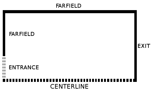
(a) Lateral view of boundary conditions.

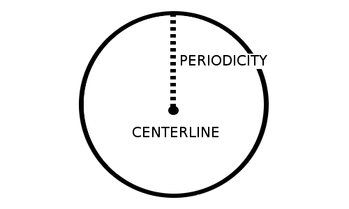
(b) Frontal view of boundary conditions.

Figure 1: Lateral and frontal views of the computational domain indicating boundary conditions.

7.1 Far Field Boundary

Riemann invariants Long et al. [1991] are used to implement far field boundary conditions. They are derived from the characteristic relations for the Euler equations. At the interface of the outer boundary, the following expressions apply

$${\mathbf{R}^{-}={\mathbf{R}}_{\infty}^{-}} {=} {q_{n_{\infty}}-\frac{2}{\gamma-1}a_{\infty}\,\mbox{,}}$$ (73)

$${\mathbf{R}^{+}={\mathbf{R}}_{e}^{+}} {=} {q_{n_{e}}-\frac{2}{\gamma-1}a_{e}\,\mbox{,}}$$ (74)

where $\infty$ and $e$ indexes stand for the property in the freestream and in the internal region, respectively. $q_{n}$ is the velocity component normal to the outer surface, defined as

$${q_{n}={\bf u}\cdot\vec{n}\,\mbox{,}}$$ (75)

and $\vec{n}$ is the unit outward normal vector

$${\vec{n}\,=\,[n_{x}\,\,n_{y}\,\,n_{z}]^{T}\,=\,\frac{1}{\sqrt{\eta_{x}^{2}+\eta_{y}^{2}+\eta_{z}^{2}}}[\eta_{x}\ \eta_{y}\ \eta_{z}]^{T}\,\mbox{.}}$$ (76)

Equation (76) assumes that the $\eta$ direction is pointing from the jet to the external boundary. Solving for $q_{n}$ and $a$, one can obtain

$${q_{nf}=\frac{\mathbf{R}^{+}+\mathbf{R}^{-}}{2}\,\mbox{,}} {a_{f}=\frac{\gamma-1}{4}(\mathbf{R}^{+}-\mathbf{R}^{-})\,\mbox{.}}$$ (77)

The $f$ index is linked to the property at the boundary surface and it is used to update the solution at this boundary. For a subsonic exit boundary, $0<q_{n_{e}}/a_{e}<1$, the velocity components are derived from internal properties as

$${u_{f}} {=} {u_{e}+(q_{nf}-q_{n_{e}})\,n_{x}\,\mbox{,}}$$

$${v_{f}} {=} {v_{e}+(q_{nf}-q_{n_{e}})\,n_{y}\,\mbox{,}}$$ (78)

$${w_{f}} {=} {w_{e}+(q_{nf}-q_{n_{e}})\,n_{z}\,\mbox{.}}$$

Density and pressure are obtained by extrapolating the entropy from the adjacent grid node,

$${\rho_{f}=\left(\frac{\rho_{e}^{\gamma}a_{f}^{2}}{\gamma p_{e}}\right)^{\frac{1}{\gamma-1}}\,\mbox{,}} {p_{f}=\frac{\rho_{f}a_{f}^{2}}{\gamma}\,\mbox{.}}$$

For a subsonic entrance, $-1<q_{n_{e}}/a_{e}<0$, properties are obtained similarly from the freestream variables as

$${u_{f}} {=} {u_{\infty}+(q_{nf}-q_{n_{\infty}})\,n_{x}\,\mbox{,}}$$

$${v_{f}} {=} {v_{\infty}+(q_{nf}-q_{n_{\infty}})\,n_{y}\,\mbox{,}}$$ (79)

$${w_{f}} {=} {w_{\infty}+(q_{nf}-q_{n_{\infty}})\,n_{z}\,\mbox{,}}$$

$${\rho_{f}=\left(\frac{\rho_{\infty}^{\gamma}a_{f}^{2}}{\gamma p_{\infty}}\right)^{\frac{1}{\gamma-1}}\,\mbox{.}}$$ (80)

For a supersonic exit boundary, $q_{n_{e}}/a_{e}>1$, the properties are extrapolated from the interior of the domain as

$${\rho_{f}} {=} {\rho_{e}\,\mbox{,}}$$

$${u_{f}} {=} {u_{e}\,\mbox{,}}$$

$${v_{f}} {=} {v_{e}\,\mbox{,}}$$ (81)

$${w_{f}} {=} {w_{e}\,\mbox{,}}$$

$${e_{f}} {=} {e_{e}\,\mbox{,}}$$

and for a supersonic entrance, $q_{n_{e}}/a_{e}<-1$, the properties are extrapolated from the freestream variables as

$${\rho_{f}} {=} {\rho_{\infty}\,\mbox{,}}$$

$${u_{f}} {=} {u_{\infty}\,\mbox{,}}$$

$${v_{f}} {=} {v_{\infty}\,\mbox{,}}$$ (82)

$${w_{f}} {=} {w_{\infty}\,\mbox{,}}$$

$${e_{f}} {=} {e_{\infty}\,\mbox{.}}$$

7.2 Entrance Boundary

For a jet-like configuration, the entrance boundary is divided in two areas: the jet and the area above it. The jet entrance boundary condition is implemented through the use of the 1-D characteristic relations for the 3-D Euler equations for a flat velocity profile. The set of properties, then, determined is computed from within and from outside the computational domain. For the subsonic entrance, the $v$ and $w$ components of the velocity are extrapolated by a zero-order extrapolation from inside the computational domain and the angle of flow entrance is assumed fixed. The remaining properties are obtained as a function of the jet Mach number, which is a known variable.

$${\left(u\right)_{1,j,k}} {=} {u_{j}\,\mbox{,}}$$

$${\left(v\right)_{1,j,k}} {=} {\left(v\right)_{2,j,k}\,\mbox{,}}$$ (83)

$${\left(w\right)_{1,j,k}} {=} {\left(w\right)_{2,j,k}\,\mbox{.}}$$

The dimensionless total temperature and total pressure are defined with the isentropic relations:

$${T_{t}=1+\frac{1}{2}(\gamma-1)M_{j}^{2}\,} {P_{t}=\frac{1}{\gamma}(T_{t})^{\frac{\gamma}{\gamma-1}}\,\mbox{.}}$$ and (84)

The dimensionless static temperature and pressure are deduced from Eq. (84), resulting in

$${\left(T\right)_{1,j,k}=\frac{T_{t}}{1+\frac{1}{2}(\gamma-1)(u^{2}+v^{2}+w^{2})_{1,j,k}}\,} {\left(p\right)_{1,j,k}=\frac{1}{\gamma}(T)_{1,j,k}^{\frac{\gamma}{\gamma-1}}\,\mbox{.}}$$ and (85)

For the supersonic case, all conserved variables receive the jet property values. Such entrance boundary conditions do not include any disturbance to the inlet velocity. The present approach simply generates a “top hat” velocity profile at the jet entrance. The calculations performed in the context of this work have indicated, at least for the cases addressed here, that numerical disturbances already present in the solution process are sufficient to destabilize the flow and induce turbulence transition in the jet.

The far field boundary conditions are implemented outside of the jet area in order to correctly propagate information coming from the inner domain of the flow to the outer regions of the simulation. However, in the present case, $\xi$, instead of $\eta$, as presented in the previous subsection, is the normal direction used to define the Riemann invariants.

7.3 Exit Boundary Conditions

At the exit plane, the same reasoning of the jet entrance boundary is applied. In this case, for a subsonic exit, the pressure is obtained from the outside, i.e., it is assumed given, and all other variables are extrapolated from the interior of the computational domain by a zero-order extrapolation. The conserved variables are obtained as

$${(\rho)_{I_{MAX},j,k}} {=} {\frac{(p)_{I_{MAX},j,k}}{(\gamma-1)(e_{i})_{I_{MAX}-1,j,k}}\mbox{,}}$$ (86)

$${(\vec{u})_{I_{MAX},j,k}} {=} {(\vec{u})_{I_{MAX}-1,j,k}\mbox{,}}$$ (87)

$${(e)_{I_{MAX},j,k}} {=} {(\rho)_{I_{MAX},j,k}\left[(e_{i})_{I_{MAX}-1,j,k}+\frac{1}{2}(\vec{u})_{I_{MAX},j,k}\cdot(\vec{u})_{I_{MAX},j,k}\right]\,\mbox{,}}$$ (88)

in which $I_{MAX}$ stands for the last point of the mesh in the axial direction. For the supersonic exit, all properties are extrapolated from the interior domain.

7.4 Centerline Boundary Conditions

The centerline boundary is a singularity of the coordinate transformation and, hence, an adequate treatment of this boundary must be provided. The conserved properties are extrapolated from the adjacent longitudinal plane and they are averaged in the azimuthal direction in order to define the updated properties at the centerline of the jet.

The fourth-difference terms of the artificial dissipation scheme, used in the present work, are carefully treated in order to avoid the five-point difference stencils at the centerline singularity. If one considers the flux balance at one grid point near the centerline boundary in a certain coordinate direction, let $w_{j}$ denote a component of the $\mathcal{W}$ vector from Eq. (66) and $\mathbf{d}_{j}$ denote the corresponding artificial dissipation term at the $j$-th mesh point. In the present example, $\left(\Delta w\right)_{j+\frac{1}{2}}$ stands for the difference between the solution at the interface for the points $j+1$ and $j$. The fourth-difference of the dissipative fluxes from Eq. (6.1) can be written as

$${\mathbf{d}_{j+\frac{1}{2}}=\left(\Delta w\right)_{j+\frac{3}{2}}-2\left(\Delta w\right)_{j+\frac{1}{2}}+\left(\Delta w\right)_{j-\frac{1}{2}}\,\mbox{.}}$$ (89)

Considering the centerline and the point $j=1$, as presented in Fig. 2, the calculation of $\mathbf{d}_{1+\frac{1}{2}}$ demands the $\left(\Delta w\right)_{\frac{1}{2}}$ term, which is unknown since it is outside the computation domain. In the present work a extrapolation is performed and given by

$${\left(\Delta w\right)_{\frac{1}{2}}=-\left(\Delta w\right)_{1+\frac{1}{2}}\,\mbox{.}}$$ (90)

This extrapolation modifies the calculation of $\mathbf{d}_{1+\frac{1}{2}}$ that can be written as

$${\mathbf{d}_{j+\frac{1}{2}}=\left(\Delta w\right)_{j+\frac{3}{2}}-3\left(\Delta w\right)_{j+\frac{1}{2}}\,\mbox{.}}$$ (91)

The approach is plausible since the centerline region is smooth and does not have high gradient of properties.

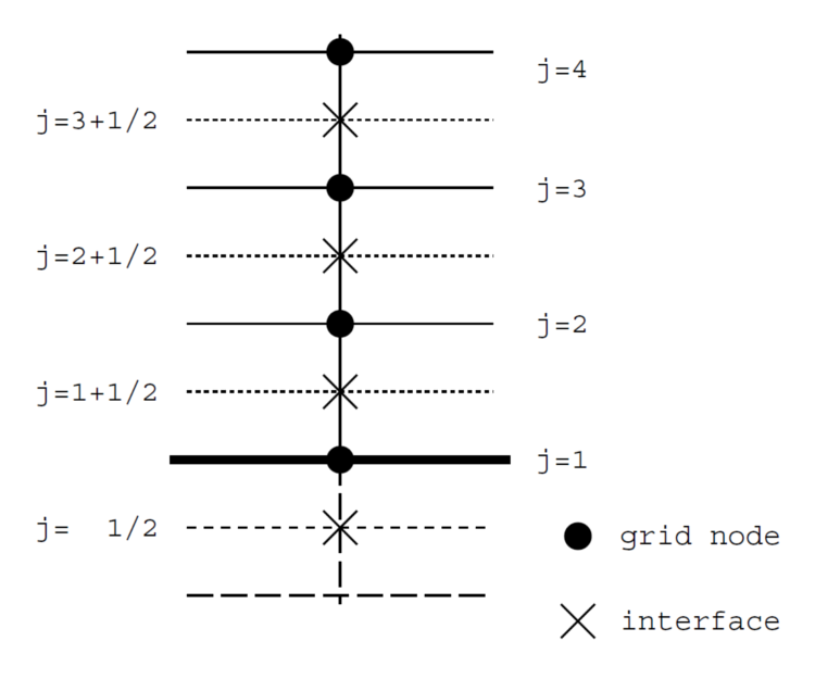
Figure 2: Boundary point dissipation operator at centerline Bigarella [2002].

7.5 Periodic Boundary Conditions

A periodic condition is implemented between the first ($K=1$) and the last point in the azimuthal direction ($K=K_{MAX}$) in order to close the 3-D computational domain. There are no boundaries in this direction, since all the points are inside the domain. The first and the last points, in the azimuthal direction, are superposed in order to facilitate the boundary condition implementation which is given by

$${(\rho)_{i,j,K_{MAX}}} {=} {(\rho)_{i,j,1}\,\mbox{,}}$$

$${(u)_{i,j,K_{MAX}}} {=} {(u)_{i,j,1}\,\mbox{,}}$$

$${(v)_{i,j,K_{MAX}}} {=} {(v)_{i,j,1}\,\mbox{,}}$$ (92)

$${(w)_{i,j,K_{MAX}}} {=} {(w)_{i,j,1}\,\mbox{,}}$$

$${(e)_{i,j,K_{MAX}}} {=} {(e)_{i,j,1}\,\mbox{.}}$$

8 Study of Supersonic Jet Flow

Four test cases are addressed in the present work in order to study the use of 2nd-order spatial discretization on large eddy simulations of a perfectly expanded jet flow configuration. These test cases compare the effects of mesh refinement and SGS models on the results. Two different meshes are created for the grid refinement study. Results for the three SGS models implemented in the code, namely, classic Smagorinsky, dynamic Smagorinsky and Vreman models, are compared in the current section. The present results are compared with analytical, numerical and experimental data from the literature Bridges and Wernet [2008], Mendez et al. [2010, 2012].

8.1 Geometry Characteristics

Two different computational domain geometries are created for the jet simulations discussed in the current work. One geometry presents a cylindrical shape and the other one presents a divergent conical shape. For the sake of simplicity, the cylindrical geometry is named geometry A and the other one is named geometry B in the present paper. The computational domains are created in two steps. First, a 2-D region is generated. In the sequence, this region is rotated about the jet axis in order to generate a fully 3-D geometry. An in-house code is used for the generation of the 2-D domain of geometry A. The commercial mesh generator ANSYS^® ICEM CFD ANSYS [2016] is used for the 2-D domain of geometry B.

Geometry A is a cylindrical domain with radius of $20D$ and a length of $50D$. Geometry B presents a divergent form whose axis length is $40D$. The minimum and maximum heights of geometry B are $\approx 16D$ and $25D$, respectively. Geometry B is created based on results from simulations using geometry A in order to refine the mesh in the shear layer region of the jet flow. The 2-D coordinates of the zones created for geometry B and further details of the geometry can be found in Ref. Junqueira-Junior [2016]. Geometries A and B are illustrated in Fig. 3 which presents a 3-D view of the two computational domains used in the current work. The geometries are colored by an instantaneous visualization of the solution for the axial component of the flow velocity.

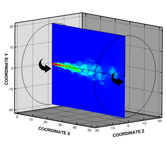
(a) 3-D view of two XZ planes of geometry A.

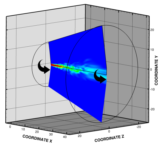
(b) 3-D view of two XZ planes of geometry B.

Figure 3: 3-D view of computational domain geometries used for the LES calculations.

8.2 Mesh Configurations

One grid is generated for each geometry used in the present study. These computational grids are named mesh A and mesh B. An illustration of the computational grids is presented in Fig. 4.

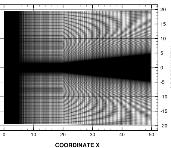
(a) 2-D view of mesh A in the XZ plane.

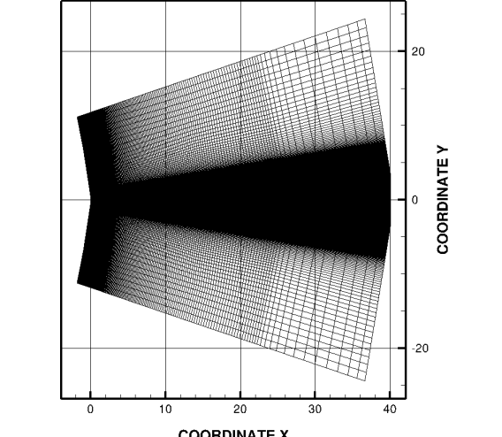
(b) 2-D view of mesh B in the XZ plane.

Figure 4: 2-D view of the computational meshes used in the present work.

Mesh A is created using a mesh generator developed by the research group for the cylindrical shape configuration, i.e., geometry A. This computational mesh is composed of 400 points in the axial direction, 200 points in the radial direction and 180 points in the azimuthal direction, which yields a total of 14.4 million grid points. Hyperbolic tangent functions are used for the point distributions in the radial and axial directions. Grid points are clustered near the shear layer of the jet. The mesh is coarsened towards the outer regions of the domain in order to dissipate properties of the flow far from the jet. Such mesh refinement approach can avoid the reflection of waves back into the domain.

The radial and longitudinal dimensions of the smallest distance between mesh points of grid A are given by $(\Delta\underline{r})_{min}=0.002D$ and $(\Delta\underline{x})_{min}=0.0126D$, respectively. This minimal spacing occurs at the shear layer of the jet and at the entrance of the computational domain. Mesh A characteristics are chosen based on data provided by the work of Mendez et al. Mendez et al. [2010, 2012], who have also used a second-order accurate spatial discretization scheme for the same jet flow configuration. Simulations were initially performed using mesh A. This particular calculation has used the static Smagorinsky SGS model, and details of the calculation are discussed in the forthcoming sections. The results indicated that further grid refinement was necessary and they also helped in the decision of which regions of the domain should be refined. Therefore, the authors created a second computational grid, mesh B, which also adopted a somewhat different topology for the computational domain, geometry B, as previously discussed.

The more refined computational grid, mesh B, is composed of 343 points in the axial direction, 398 points in the radial direction and 360 points in the azimuthal direction. This yields a mesh with approximately 50 million grid points. The 2-D mesh is generated with ANSYS^® ICEM CFD ANSYS [2016]. The points are allocated using different distributions in eight edges of the 2-D domain. The same coarsening approach used for mesh A is also applied for mesh B. The distance between mesh points increases towards the outer region of the domain. This procedure forces the dissipation of properties far from the jet in order to avoid reflection of waves into the domain. The grid coarsening can be understood as an implicit damping which can smooth out properties far from the jet, in the region where the mesh is no longer refined. Figure 5 illustrates the edges used to generate the point distribution and the direction of the mesh coarsening. Table 1 presents the number of points, the growth factor and the smallest grid spacing for all auxiliary edges used to generate the mesh.

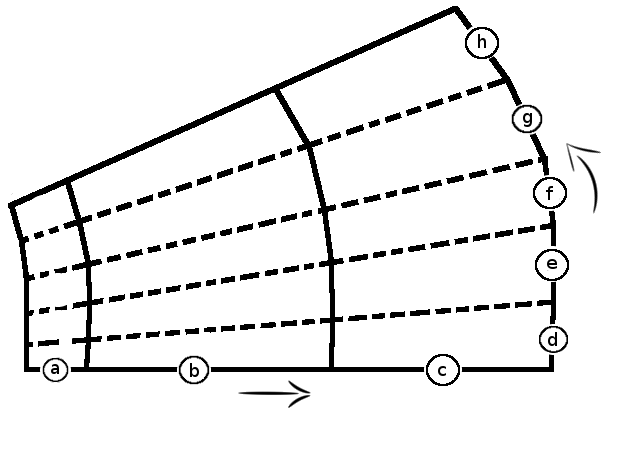
Figure 5: Auxiliary edges used for the generation of mesh B.

Table 1: Characteristics of mesh B.

Edge	Nb. of points	Growth Factor	Smallest Spacing
a	300	1.01912	$1.000\times 10^{-3}$ D
b	30	1.02739	$2.8231\times 10^{-1}$ D
c	15	1.30370	$3.4482\times 10^{-1}$ D
d	45	1.00	$3.40909\times 10^{-3}$ D
e	155	1.03724	$3.40909\times 10^{-3}$ D
f	155	1.01034	$1.18655\times 10^{-2}$ D
g	40	1.07161	$5.73327\times 10^{-2}$ D
h	7	1.08206	$7.93887\times 10^{-1}$ D

8.3 Flow Configuration and Boundary Conditions

An unheated perfectly expanded jet flow is chosen to perform the present studies with the LES tool. The jet entrance Mach number is $1.4$. The pressure ratio, $PR=P_{j}/P_{\infty}$, and the temperature ratio, $TR=T_{j}/T_{\infty}$, between the jet entrance and the ambient freestream conditions, are equal to one, i.e., $PR=1$ and $TR=1$. The Reynolds number of the jet is $Re=1.57\times 10^{6}$, based on the jet entrance diameter, D. This flow configuration is chosen due to the absence of strong shocks waves. Strong discontinuities clearly create additional numerical difficulties, that the authors did not want to add to the present study. Moreover, numerical and experimental data are available in the literature for this flow configuration, such as the work of Mendez et al. Mendez et al. [2010, 2012] and the work of Bridges and Wernet Bridges and Wernet [2008].

The boundary conditions discussed in Sect. 7 are used in the simulations performed in the present paper. Figure 1 presented a lateral view and a frontal view of the computational domain used for the simulations, indicating the positioning of each boundary condition. A top hat velocity profile, with $M=1.4$, is used at the entrance boundary. Riemann invariants are used at the stagnated ambient regions. A special singularity treatment is performed at the centerline. Periodicity is imposed in the azimuthal direction. Properties of flow at the inlet and at the farfield regions have to be provided to the code in order to impose the boundary conditions. Density, $\rho$, temperature, $T$, velocity, $U$, Reynolds number, $Re$, and specific heat at constant volume, $C_{v}$, are provided in the dimensionless form to the simulation. These properties are given by

$$\rho_{j}=1.00\,\mbox{,} \rho_{\infty}=1.00\,\mbox{,}$$

$$T_{j}=1.00\,\mbox{,} T_{\infty}=1.00\,\mbox{,}$$ (93)

$$U_{j}=1.4\,\mbox{,} U_{\infty}=0.00\,\mbox{,}$$

$$Re_{j}=1.57\times 10^{6}\,\mbox{,} C_{v}=1.786\,\mbox{,}$$

where the $j$ subscript identifies the properties at the jet entrance and the $\infty$ subscript stands for properties at the farfield region.

8.4 Large Eddy Simulations

Four simulations are performed in the present work. The objective is to study the effects of mesh refinement and to evaluate the three different SGS models included into the code. The calculations are performed in two steps. First, a preliminary simulation is performed in order to achieve a statistically steady state condition. In the sequence, the simulations are run for another period in order to collect enough data for the calculation of time averaged properties of the flow and their fluctuations.

8.4.1 Statistically Steady Flow Condition

The configurations of all simulations are discussed in the current subsection towards the description of the preliminary calculations which are performed in order to drive the flow to a statistically steady flow condition. In this preliminary stage, the goal is to achieve a starting point to begin the calculation of statistical data. Table 2 presents the operating conditions of all four numerical studies performed in the current research. S1, S2 and S3 simulations were the test cases that admitted stagnated flow conditions as the initial conditions for the preliminary simulations. Differently from the former studies, the S4 simulation used the statistically steady state condition of the S2 computational study as initial condition for this preliminary stage. Mesh A is only used in the S1 simulation. The other calculations are performed using the more refined grid, Mesh B. S1, S2, S3 and S4 studies apply, respectively, time increments of $2.5\times 10^{-5}$, $1.0\times 10^{-4}$, $5.0\times 10^{-5}$ and $1.0\times 10^{-4}$, in dimensionless time units, as indicated in the 4th column of Tab. 2. The dimensionless time increment used for all configurations is the largest one which the solver can handle without diverging the solution. The static Smagorinsky model Lilly [1965, 1967], Smagorinsky [1963] is used in the S1 and S2 simulations. The dynamic Smagorinsky model Germano et al. [1991], Moin et al. [1991] and the Vreman model Vreman [2004] are used in simulations S3 and S4, respectively.

The total (physical) time simulated by all numerical studies in order to achieve the statistically steady state condition is indicated in the 6th column of Tab. 2 in flow through time (FTT) units. One flow through time is the necessary amount of time for a particle to cross all the domain considering the inlet velocity of the jet. The S1 simulation is the least expensive test case studied and, therefore, one could afford to let it run for a longer period of time. It uses a 14 million point mesh while the other simulations use the 50 million point grid. On the other hand, simulation S3 is the most expensive numerical test case, because the dynamic Smagorinsky SGS model requires more computational time per time step when compared with the other SGS models implemented in the code. Moreover, the time step restrictions for the dynamic Smagorinsky model are much more stringent, as one can see in Tab. 2. Hence, the S3 simulation has only been run for 8.20 FTT for this study.

Table 2: Overall characteristics of the large eddy simulations performed in the present work.

Simulation	Mesh	SGS	$\Delta t$	Initial Condition	FTT
S1	A	Static Smagorinsky	$2.5\times 10^{-5}$	Stagnated flow	52.9
S2	B	Static Smagorinsky	$1\times 10^{-4}$	Stagnated flow	14.2
S3	B	Dynamic Smagorinsky	$5\times 10^{-5}$	Stagnated flow	8.20
S4	B	Vreman	$1\times 10^{-4}$	S2	19.1

8.4.2 Mean Flow Property Calculations

After the statistically stationary state is achieved, the simulations are restarted and run for another period of time in which data of the flow are extracted and recorded in a fixed frequency. The collected data are time averaged in order to calculate mean properties of the flow and compare them with the results of the numerical and experimental references. In the present section, time-averaged properties are denoted as $\langle\cdot\rangle$. Table 3 summarizes the information on data collecting and time averaging for the four test cases addressed here. The 2nd column presents the number of extractions performed during the simulations. Data are extracted each 0.02 dimensionless time units in the present work, which is equivalent to a dimensionless frequency of 50. The choice of this frequency is based on the numerical work reported in Refs. Mendez et al. [2010, 2012]. The last column of Tab. 3 presents the total additional dimensionless time simulated in order to extract the data to calculate the mean properties.

Table 3: Details of the data extraction for mean flow calculations for each test case.

Simulation	Number of Extractions	Frequency	Data Extraction Time
S1	2048	50	1.60 FTT
S2	3365	50	3.30 FTT
S3	2841	50	2.77 FTT
S4	1543	50	1.51 FTT

8.5 Study of Mesh Refinement Effects

Effects of mesh refinement on compressible LES using the JAZzY solver are discussed in the present section. Time-averaged 2-D distributions and profiles of the axial component of velocity are collected from simulations S1 and S2, and they compared with numerical and experimental results from the literature Bridges and Wernet [2008], Mendez et al. [2010, 2012]. Both simulations use the same SGS model, the static Smagorinsky model Lilly [1965, 1967], Smagorinsky [1963]. Mesh A is used on the S1 simulation while Mesh B is used on the S2 simulation. Figure 6 illustrates the positioning of surfaces and profiles extracted for all simulations performed in the present work.

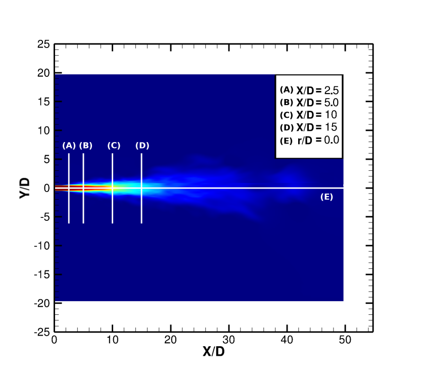
Figure 6: Positioning in the computational domain of surfaces studied in the present work.

Cuts (A) through (D) are radial profiles at different positions downstream of the jet entrance. An average in the azimuthal direction is performed when the radial profiles are calculated. The last region indicated in Fig. 6, Cut (E), represents the jet axis.

8.5.1 Time Averaged Axial Component of Velocity

One important characteristic of round jet flow configurations is the potential core length, $\delta_{j}^{95\%}$. The potential core is defined as the region in which the axial velocity component, $U_{j}^{95\%}$, is at least $95\%$ of the velocity of the jet at the inlet, i.e.,

$$U_{j}^{95\%}=0.95\,\,U_{j}\,\mbox{.}$$ (94)

Therefore, the potential core length can be defined by the point in which the mean axial velocity component reaches $U_{j}^{95\%}$ along the centerline.

Lateral views of $\langle U\rangle$ for the S1 and S2 simulations are presented in Fig. 7. In these contour plots, $U_{j}^{95\%}$ is indicated by the black solid line.

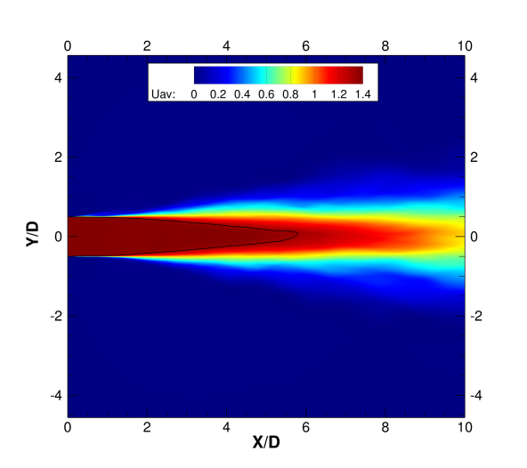
(a) Lateral view of $\langle U\rangle$ for S1 simulation.

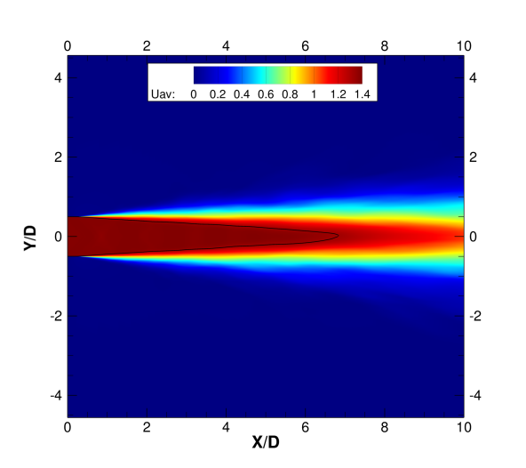
(b) Lateral view of $\langle U\rangle$ for S2 simulation.

Figure 7: Lateral view of the averaged axial component of velocity, $\langle U\rangle$, for the S1 and S2 simulations. The solid black line (–) indicates the potential core of the jet, $U_{j}^{95\%}$.

Table 4 presents the potential core length for the S1 and S2 simulations. The present calculations are compared to the numerical results from Refs. Mendez et al. [2010, 2012], both in terms of the actual values of $\delta_{j}^{95\%}$ as well as in terms of the relative error with respect to the experimental data Bridges and Wernet [2008].

Table 4: Potential core length and relative error with respect to the experimental data Bridges and Wernet [2008].

Simulation	$\delta_{j}^{95\%}$	Relative error
S1	5.57	40%
S2	6.84	26%
Mendez et al.	8.35	8%

There are significant differences between the results for the S1 and S2 test cases, as well as between those and the computational results from Ref. Mendez et al. [2012]. The results for the S1 simulation present a smaller $\delta_{j}^{95\%}$, when compared to the results for the S2 simulation, i.e., 5,57 and 6.84, respectively. The S1 solution is over dissipative when compared to the S2 results and, hence, the jet decays earlier in the S1 simulation. As previously discussed, the mesh used in the S1 test case is very coarse when compared to the grid used for the S2 simulation. This lack of spatial resolution can generate very dissipative solutions which yield the under prediction of the potential core length. The mesh refinement reduced in 14% the relative error of the S2 simulation when compared to the experimental data.

Profiles of $\langle U\rangle$ along the mainstream direction, and the evolution of $\langle U\rangle$ along the centerline are compared with numerical and experimental results in Figs. 8 and 9, respectively. The centerline is indicated as the (E) cut in Fig. 6. The dash-point line and the solid line stand for the results of the S1 and S2 test cases, respectively, in Figs. 8 and 9. The square symbols are the LES results of Mendez et al. Mendez et al. [2010, 2012], while the triangular symbols indicate the experimental data of Bridges and Wernet Bridges and Wernet [2008].

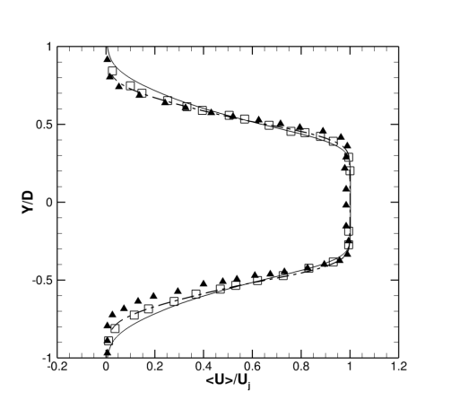
(a) X=2.5D ; $-1.5D\leq Y\leq 1.5D$

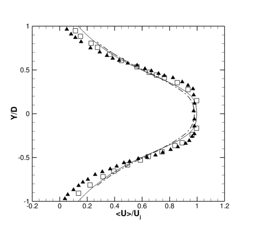
(b) X=5.0D ; $-1.5D\leq Y\leq 1.5D$

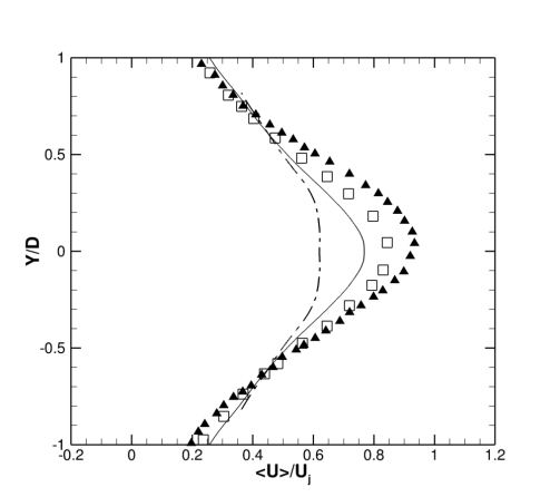
(c) X=10D ; $-1.5D\leq Y\leq 1.5D$

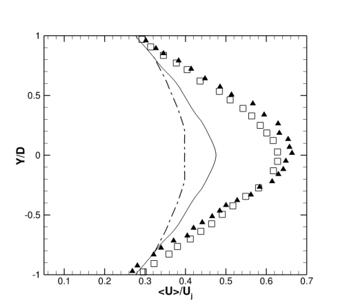
(d) X=15D ; $-1.5D\leq Y\leq 1.5D$

Figure 8: Profiles of the averaged axial component of velocity, $\langle U\rangle$, at different positions within the computational domain: (-$\cdot$-) S1 simulation; (–) S2 simulation; ($\square$) numerical data; ($\blacktriangle$) experimental data.

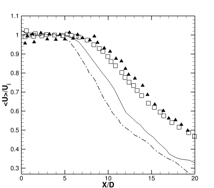
Figure 9: Evolution of the averaged axial component of velocity, $\langle U\rangle$, along the centerline (Y=0); $0\leq X\leq 20D$. (-$\cdot$-) S1 simulation; (–) S2 simulation; ($\square$) numerical data; ($\blacktriangle$) experimental data.

In compressible jet flow analisys it is very important the study the evolution of flow properties along the lipline which is defined by the region where $r/D=0.5$. The four points at the lipline from the profiles presented in Figs. 8(a), 8(b), 8(c) and 8(d) are illustrated in Fig. 10 as an evolution the averaged axial component of velocity, $\langle U\rangle$, along the lipline. A spline is used to create the curve using the four points extracted from the $\langle U\rangle$ profiles at $X/D=2.5$, $X/D=5.0$, $X/D=10$ and $X/D=15$. The black line stands for the numerical data, the red line for the experimental, the magenta line for the S1 simulation and the green line for the S2 simulation.

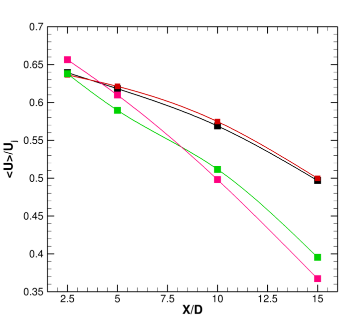
Figure 10: Extractions of the averaged axial component of velocity, $\langle U\rangle$, along the lipline (Y/D=0.5); $0\leq X\leq 20D$. ($\blacksquare$) numerical data; ( $\blacksquare$) experimental data; ($\blacksquare$) S1 simulation; ($\blacksquare$) S2 simulation.

The comparison of profiles indicates that the distributions of $\langle U\rangle$, calculated in the present work, correlate well with the reference data up to $X=5.0D$. $\langle U\rangle$ profile, calculated in the S2 case, at $X=10.0D$ is under predicted when compared with the reference profiles. However, the comparison is still quite a bit better than the one obtained for the S1 results at this axial position. One can observe that the $\langle U\rangle$ distributions along the centerline, for the S1 and S2 cases, correlate well with the reference data in the region in which there is good grid resolution. The collection of $\langle U\rangle$ magnitude from the profiles along the lipline for the S2 simulation correlates well with the reference and numerical data until $X=5.0D$. The averaged axial component of velocity calculated in S1 simulation is always understimated when compared to the same property calculated with S2 computation. However, as the mesh spacing increases, the time-averaged axial velocity component computed using S1 and S2 numerical studies starts to correlate poorly with the references.

Figure 11 presents a lateral view of an instantaneous snapshot of the pressure contours, in grey scale, superimposed by vorticity magnitude contours, in color, for both S1 and S2 numerical studies. It is clear that the finer grid results, that is, the S2 simulation, provide greater details of the pressure and vorticity fields.

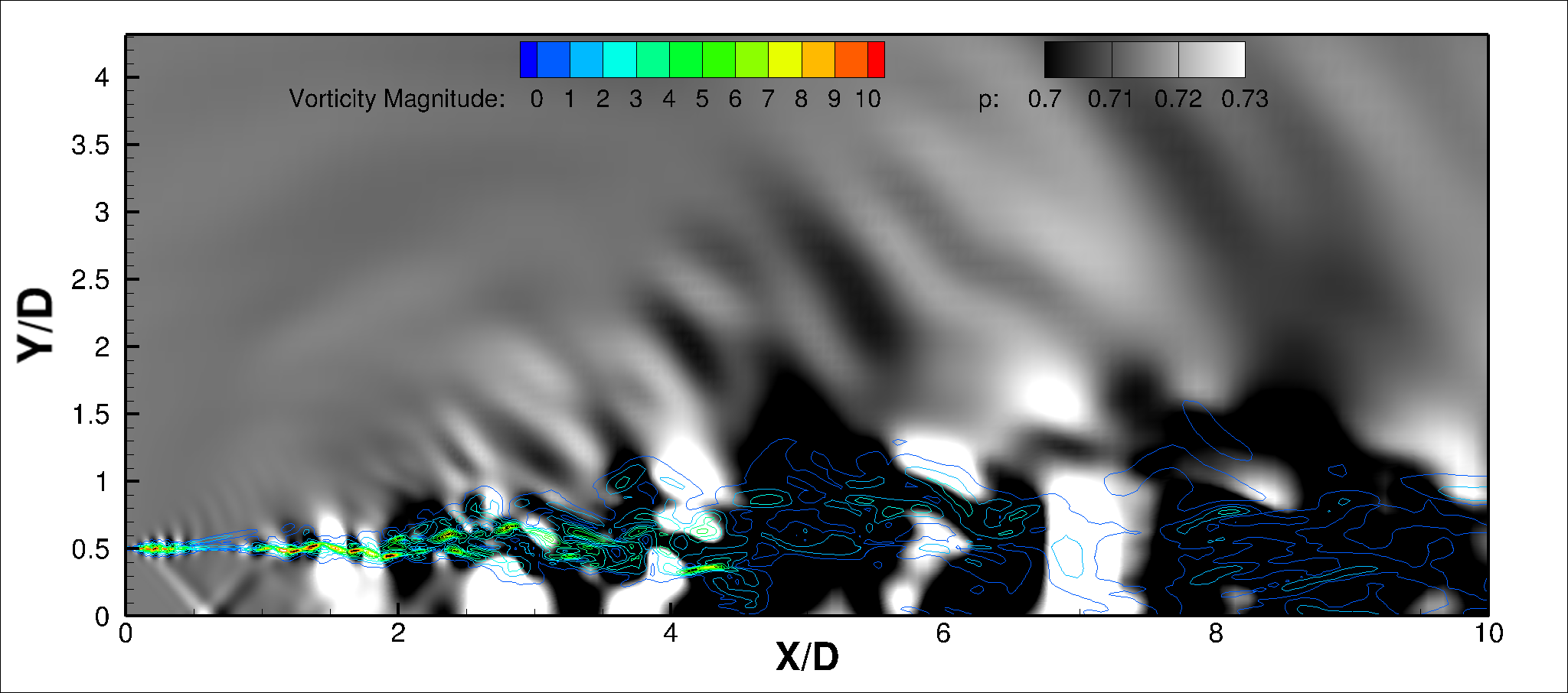
(a) S1 simulation.

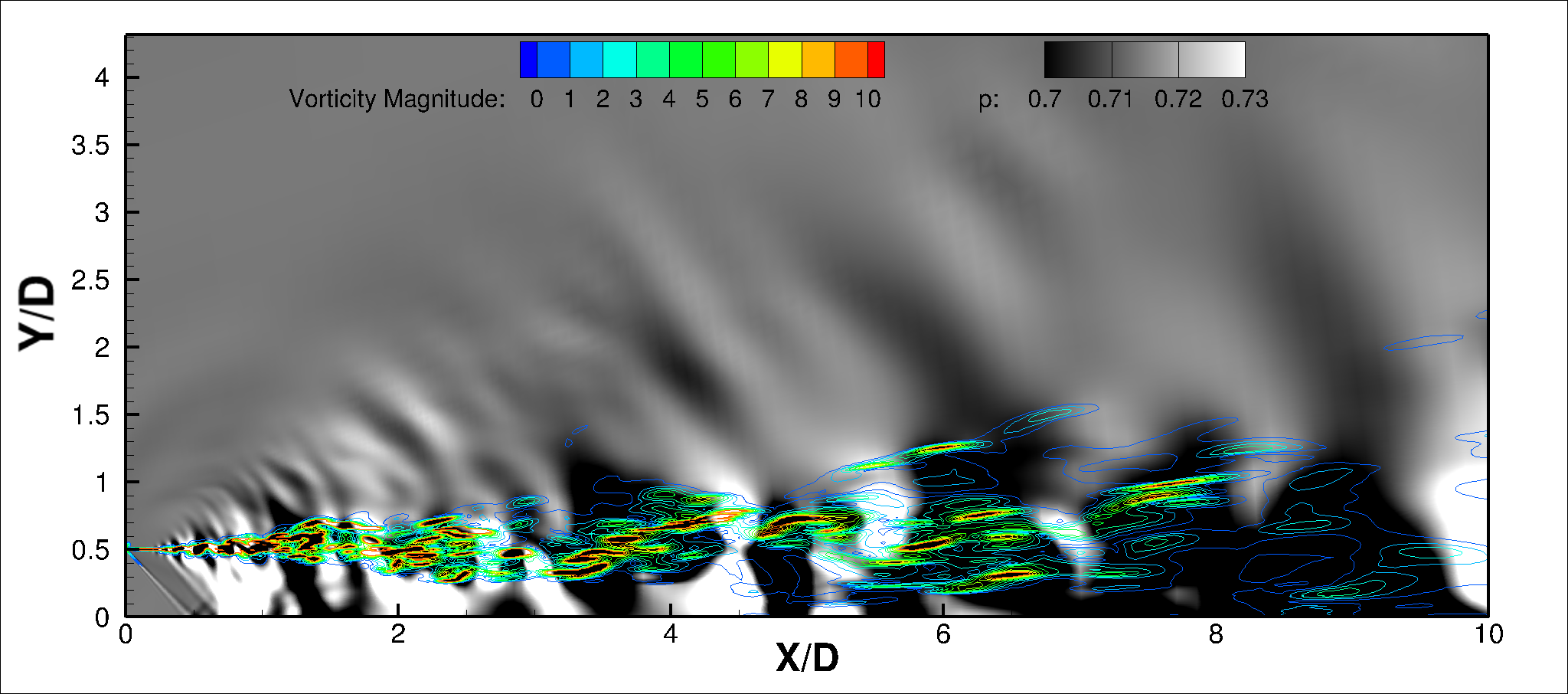
(b) S2 simulation.

Figure 11: Lateral view of instantaneous pressure contours, in grey scale, superimposed by vorticity magnitude contours, in color, of the jet flow computed in the S1 and S2 simulations.

A detailed visualization of the jet entrance is shown in Fig. 12, for the two test cases. As before, an instantaneous snapshot of one longitudinal plane of the jet flow is shown. Pressure contours are shown as a background visualization in grey scale, and this is superimposed by vorticity magnitude contours, in color. The better resolution of flow features obtained for the S2 test case is even more evident in this detailed plot of the jet entrance. In particular, compression waves generated at the shear layer, and their reflections at the jet axis, are much more clearly visible in the S2 results. At the end, this simulation provides a much richer visualization of flow features.

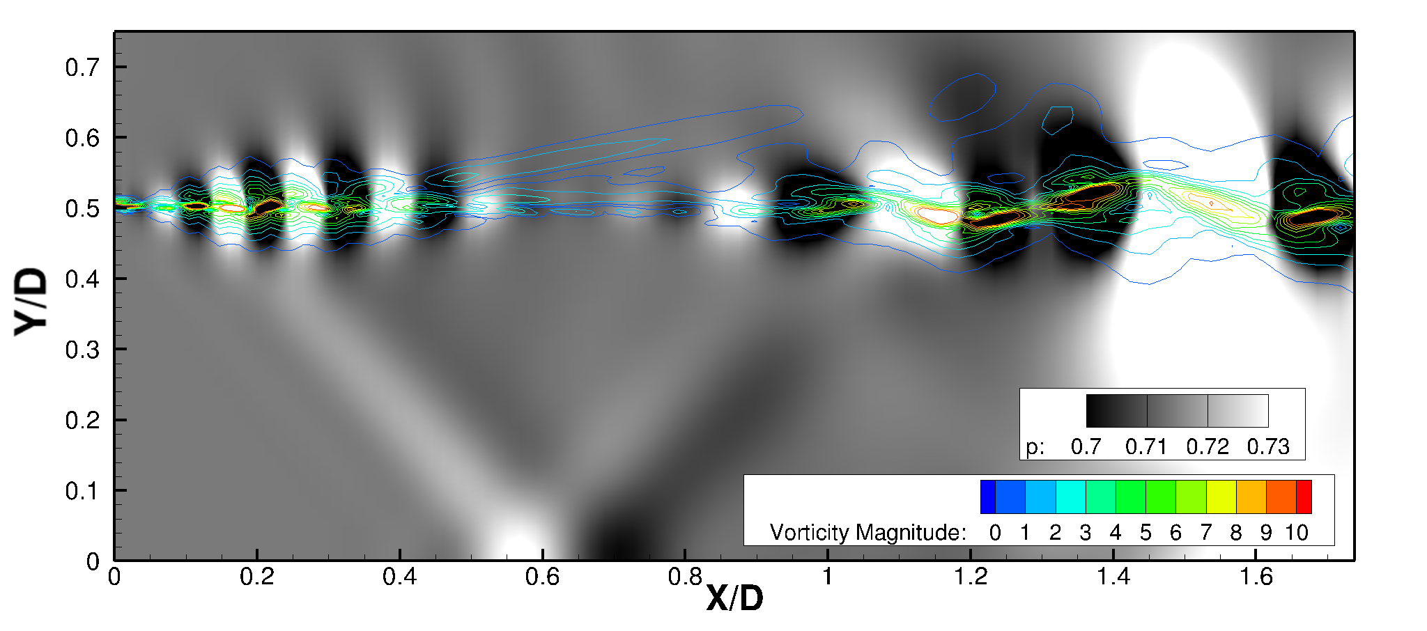
(a) S1 simulation.

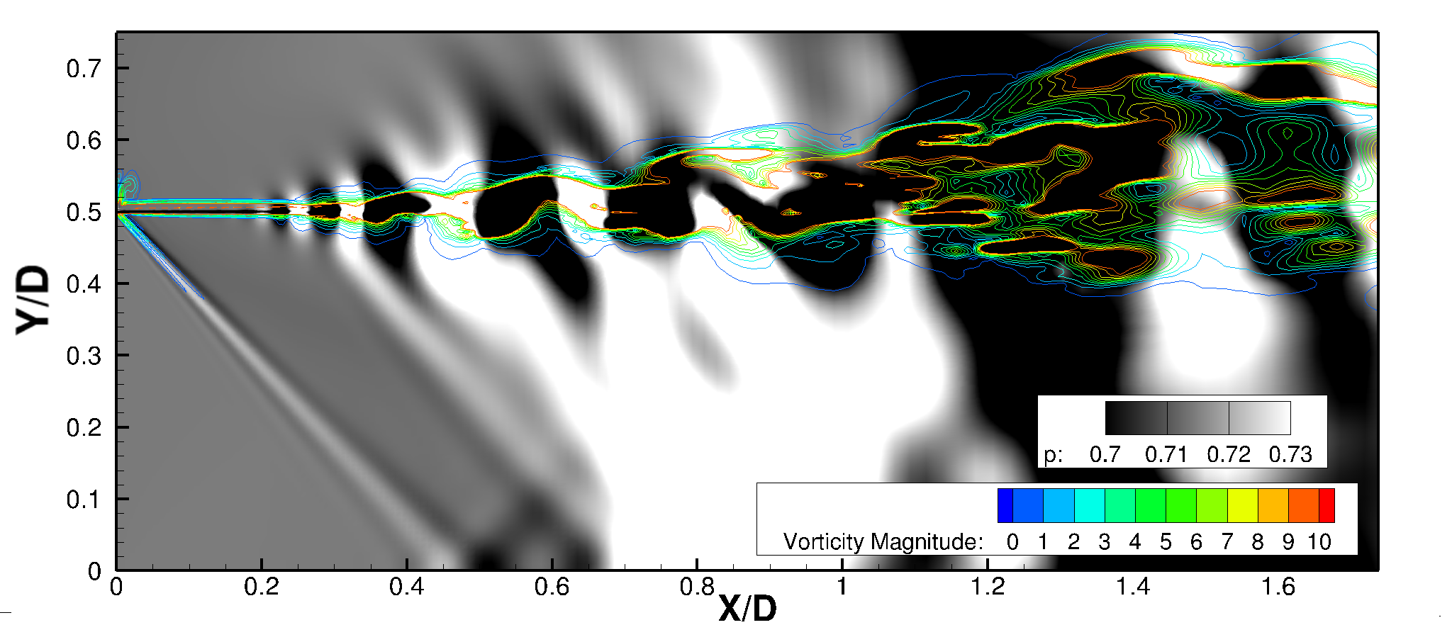
(b) S2 simulation.

Figure 12: Detailed view near the jet entrance of pressure contours, in grey scale, superimposed by vorticity magnitude contours, in color, for the S1 and S2 simulations.

8.5.2 RMS Distributions of Time Fluctuations of Axial Velocity Component

The time fluctuating part of the flow is also important to be studied. Therefore, the analysis of the effects of mesh refinement is also performed for the fluctuating part of the axial velocity component using the root mean square approach. A lateral view, i.e., a complete longitudinal plane, and a detailed view of the region near the jet entrance the root mean square (RMS) values of the fluctuating part of the axial velocity component, $u^{*}_{RMS}$, computed in the S1 and S2 simulations, are presented in Fig. 13.

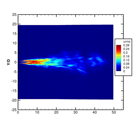
(a) $u^{*}_{RMS}$ for S1 simulation.

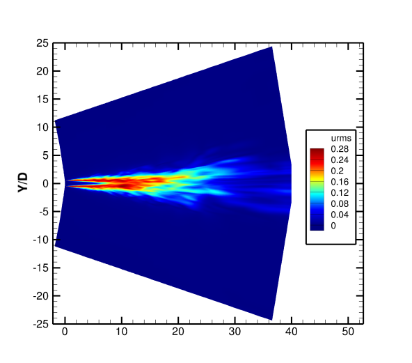
(b) $u^{*}_{RMS}$ for S2 simulation.

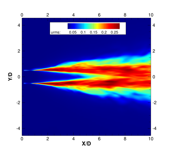
(c) $u^{*}_{RMS}$ for S1 simulation.

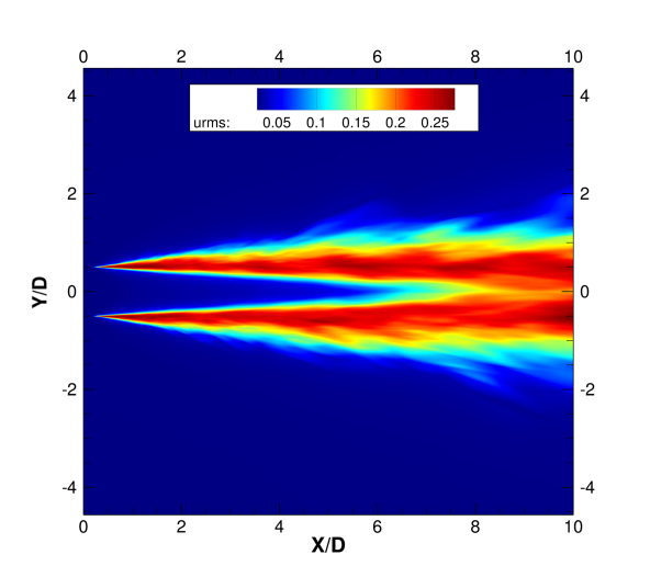
(d) $u^{*}_{RMS}$ for S2 simulation.

Figure 13: Lateral and detailed views of the RMS values of the time fluctuation of the axial component of velocity, $u_{RMS}^{*}$, for S1 and S2 simulations.

One can observe, for instance, in Figs. 13(a) and 13(b), that the mesh coarsening in the streamwise direction, towards the farfield, is working as designed. In other words, the mesh stretching destroys structures of the flow towards the exit boundary and, therefore, there are no wave reflections back into the computational domain. As previously discussed, coarse meshes implicitly add dissipation to the solution and, as such, they work as sponge zones in the vicinity of undisturbed flow regions. The detailed views of $u^{*}_{RMS}$, i.e., Figs. 13(c) and 13(d), indicate that the properties calculated in the S2 study provide a better definition of the potential core and of the near jet entrance region. The results for the S1 test case are more spread and indicating a much reduced potential core length. The same effect can be observed on crossflow plane visualizations of $u^{*}_{RMS}$ contours, which, however, are not shown here for the sake of brevity.

The same strategy used to compare the mean profiles of velocity is used for the study of $u^{*}_{RMS}$. Figure 14 presents the comparison of RMS profiles of $u^{*}$, from the S1 and S2 simulations, with reference results. The profile of $u^{*}_{RMS}$ calculated using the numerical approach fits very well the experimental reference profile at $X=2.5D$ near the centerline region. However, all numerical calculations overpredict the peaks of $u^{*}_{RMS}$ at the proximity of $Y=0.5D$. The profile obtained with the S2 calculation, at the same position, presents a good correlation with numerical data whereas the $u^{*}_{RMS}$ profile calculated in S1 simulation cannot correctly represent the two peaks of the profile. At $X=5.0D$, the $u^{*}_{RMS}$ profile calculated using S2 simulation is close to the profiles achieved by the references. S1 study overstimates the RMS of $u^{*}$ near the centerline region, i.e. $r/D=0.0$. The same beahavior can be observed at $X=10.0D$, where the profiles of the fluctuating part of the axial velocity component obtained in the S1 and S2 calculations start to diverge from the reference results at $-0.5D<Y<0.5D$ vicinity. At $X=15.0D$, the $u^{*}_{RMS}$ profile for the S1 calculation is completely underpredicted when compared with the profiles of $u^{*}_{RMS}$ obtained from numerical and experimental references. At the same position, the fluctuation profile from the S2 computation presents similiar magnitudes shape when compared with the numerical and references profiles of $u^{*}_{RMS}$. However, the shape of the same profile achieved using S2 computation does not match with the reference data at $X=15.0D$.

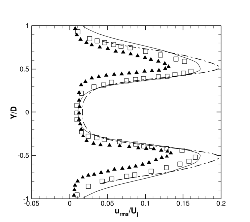
(a) X=2.5D ; $-1.5D\leq R\leq 1.5D$.

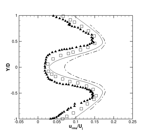
(b) X=5.0D ; $-1.5D\leq R\leq 1.5D$.

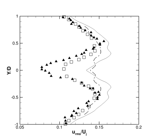
(c) X=10D ; $-1.5D\leq R\leq 1.5D$.

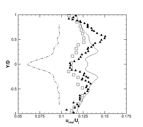
(d) X=15D ; $-1.5D\leq R\leq 1.5D$.

Figure 14: Profiles of RMS values of time fluctuation of axial component of velocity, $u_{RMS}^{*}$, for the S1 and S2 simulations, at different positions within the computational domain: (-$\cdot$-) S1; (–) S2; ($\square$) numerical data; ($\blacktriangle$) experimental data.

Figure 15 presents the distribution of $u^{*}_{RMS}$ along the centerline of the jet. The S2 calculation presents overpredicted values of $u^{*}_{RMS}$ along the centerline when compared with reference data. Nevertheless, the evolution of the same property along the centerline presents a similar shape of the evolution of $u^{*}_{RMS}$ achieved by the numerical and experimental references. One can notice that the distribution of $u^{*}_{RMS}$ along the centerline achieved by S1 calculation presents the same behavior of the distribution obtained from S2 study for $X<10D$. Both results are overpredicted when compared with the refence. However, in particular for S1 simulation, the value of $u^{*}_{RMS}$ decreases quickly in the streamwise direction for $X>10D$. This behavior of S1 calculation generates a very underpredicted distribution of $u^{*}_{RMS}$ when compared to the results of S2 simulation and refence data. Even the shape of the evolution of the property calculated by S1 simulation, for $X>10D$, along the centerline, is completely different from the evolution presented by the reference data. Therefore, it is possible to notice a significant improvement of the solution with the refinement of the mesh performed for S2 study.

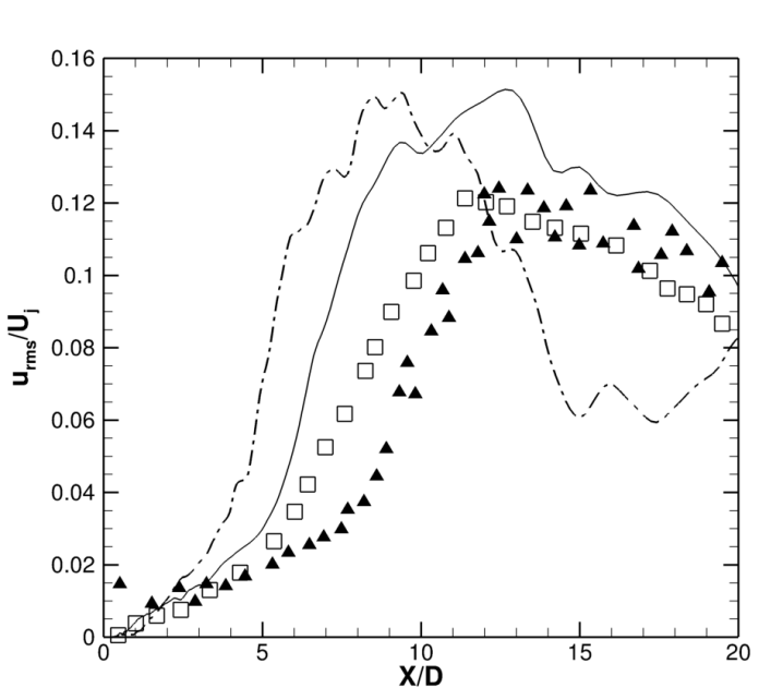
Figure 15: Evolution of RMS values of time fluctuation of axial component of velocity, $u_{RMS}^{*}$, along the centerline (Y=0); $0\leq X\leq 20D$. (-$\cdot$-) S1 simulation; (–) S2 simulation; ($\square$) numerical data; ($\blacktriangle$) experimental data.

Figure 16 presents the evolution of $u_{RMS}^{*}$ along the lipline using four points extracted from Figs. 14(a), 14(b), 14(c) and 14(d). A spline is used to create the curve using the four points extracted from the $u_{RMS}^{*}$ profiles at $X/D=2.5$, $X/D=5.0$, $X/D=10$ and $X/D=15$. The black line stands for the numerical data, the red line for the experimental, the magenta line for the S1 simulation and the green line for the S2 simulation. The peaks of $u_{RMS}^{*}$ are located near the lipline region. Figure 16 indicates that the results obtained from the numerical simulations performed in the present work and the numerical reference are overpredicted when compared with the experimental data at $X/D=2.5$ and $X/D=5.0$. The values of $u_{RMS}^{*}$ obtained by S2 calculation and the numerical reference are close to the results presented in the experimental refence at $X/D=10.0$ and $X/D=15.0$. One can notice that the results achieved using the less refined mesh in the present work fails to predict the peaks of $u_{RMS}^{*}$ at the four points compared along the lipline.

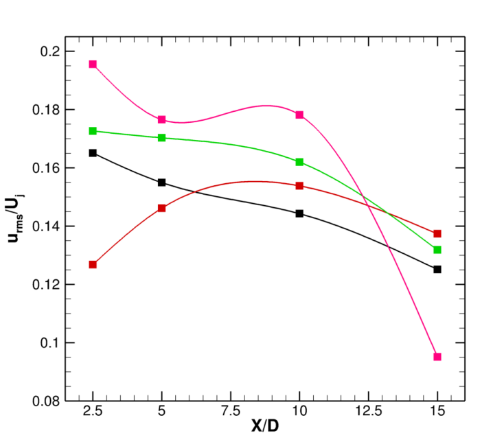
Figure 16: Extractions of RMS values of time fluctuation of axial component of velocity, $u_{RMS}^{*}$, along the lipline (Y/D=0.5); $0\leq X\leq 20D$. ($\blacksquare$) numerical data; ( $\blacksquare$) experimental data; ($\blacksquare$) S1 simulation; ($\blacksquare$) S2 simulation.

8.6 Subgrid Scale Modeling Study

After the mesh refinement study, the three SGS models added to the solver are compared. S2, S3 and S4 simulations are performed using the static Smagorinsky model Smagorinsky [1963], Lilly [1965, 1967], the dynamic Smagorinsky model Germano [1990], Moin et al. [1991] and the Vreman model Vreman [2004], respectively. The same mesh with 50 million points is used for all three simulations. The stagnated flow condition is used as intial condition for S2 and S3 simulations. A restart of S2 simulation is used as initial condition for the S4 simulation. The configuration of the numerical studies is presented at Tab. 2. An extensive comparison study is perfomed in this subsection. Time-averaged distributions of the axial and radial velocity components and eddy viscosity are presented in the subsection along with the RMS distribution of axial and radial components of velocity and distributions of the $\langle u^{*}v^{*}\rangle$ component of the Reynolds stress tensor.

8.6.1 Time Averaged Axial Component of Velocity

Effects of the SGS modeling on the time averaged results of the axial component of velocity are presented in the subsection. A lateral view of $\langle U\rangle$ for S2, S3 and S4 simulations, side by side, are presented in Fig. 17, where $U_{j}^{95\%}$ is indicated by the solid line.

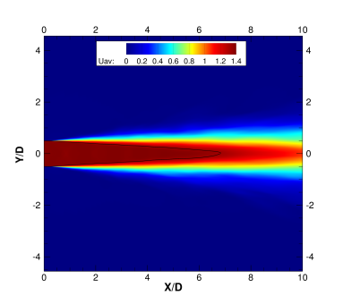
(a) Lateral view of $\langle U\rangle$ for simulation S2.

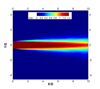
(b) Lateral view of $\langle U\rangle$ for simulation S3.

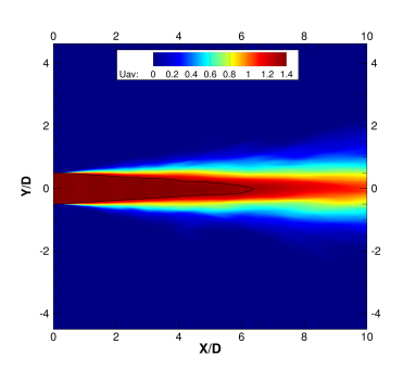
(c) Lateral view of $\langle U\rangle$ for simulation S4.

Figure 17: Lateral view of the averaged axial component of velocity, $\langle U\rangle$, for S2, S3 and S4 simulations. (–) indicates the potential core of the jet, $U_{j}^{95\%}$.

Table 5 presents the size of the potential core of S2, S3 and S4 simulations and the numerical reference Mendez et al. [2010, 2012] along with the relative error compared with the experimental data Bridges and Wernet [2008].

Table 5: Potential core length and relative error of S2, S3 and S4 simulations.

Simulation	$\delta_{j}^{95\%}$	Relative error
S2	6.84	26%
S3	6.84	26%
S4	6.28	32%
Mendez et al.	8.35	8%

Comparing the results, one cannot observe significant differences on the potential core length between S2, S3 and S4 simulations. The distribution of $\langle U\rangle$ calculated using the dynamic Smagorinky model has shown to be slightly more concentrated at the centerline region. S2 and S4 simulations time averaged distribution of $U$ are, on some small scale, more spread than the distribution obtained by S3 simulation. Figure 18 presentes instantaneous fields of pressure, in grey scale, colored by the vorticity magnitude for the numerical simulations performed with the more refined grid, Mesh B. Although the comparison is only qualitative, one cannot notice a significative effect of the SGS on the pressure fields and vorticity magnitude of the flow.

(a) S2 simulation.

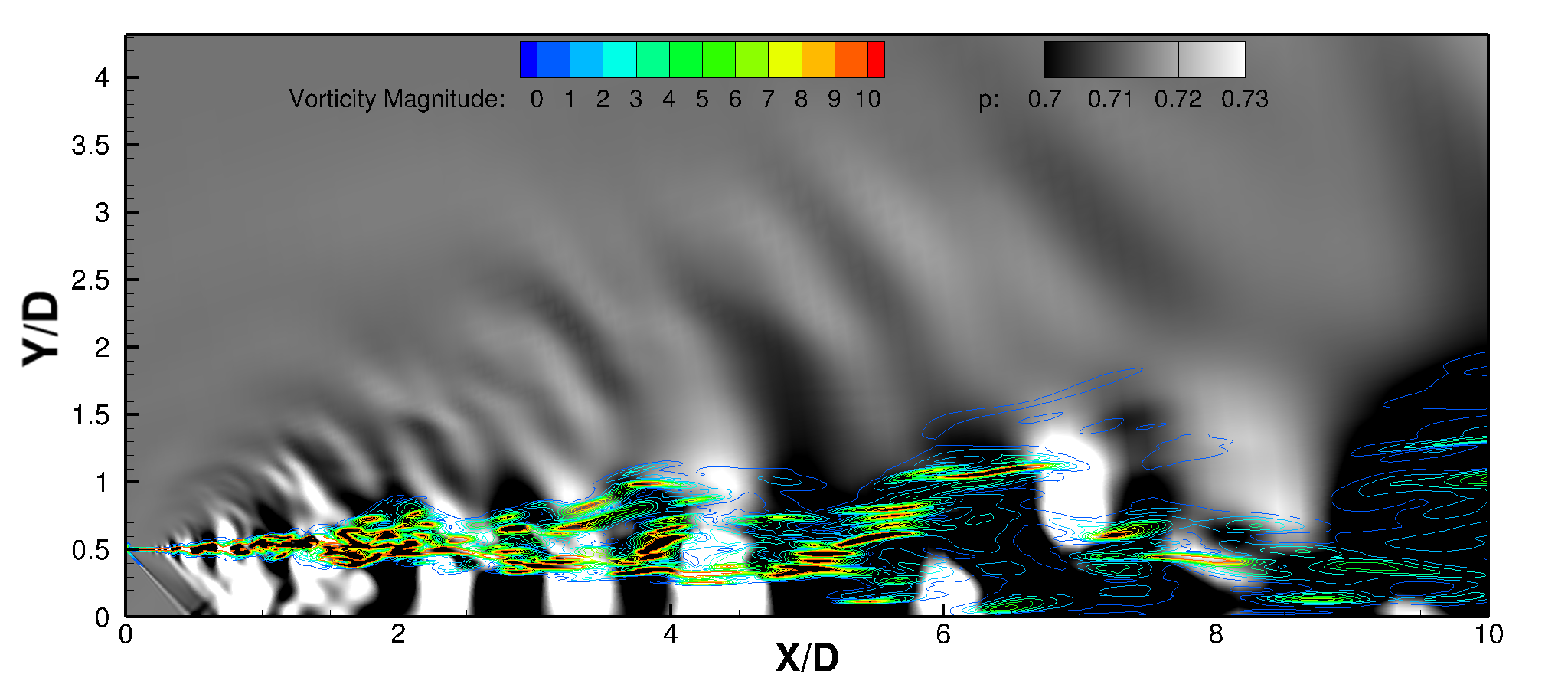
(b) S3 simulation.

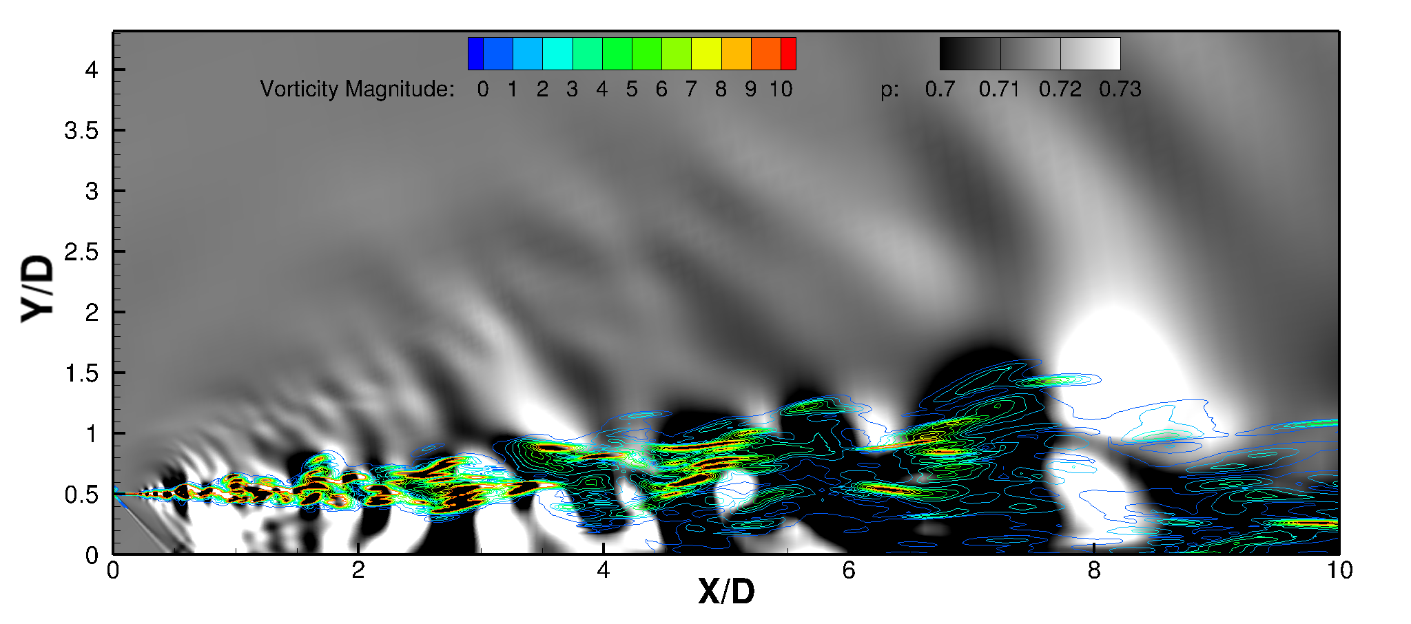
(c) S4 simulation.

Figure 18: Lateral view of field of snapshot of pressure, in grey scale, colored by the vorticity magnitude of the jet flow for S2, S3 and S4 simulations.

Profiles of $\langle U\rangle$ from S2, S3 and S4 simulations, along the mainstream direction are compared with numerical and experimental results in Fig.  19. The evolution of $\langle U\rangle$ along the centerline is illustrated in Fig. 20. The solid line, the dashed line and the circular symbol stand for the profiles of $\langle U\rangle$ computed by S2, S3 and S4 simulations, respectively. The reference data are represented by the same symbols presented in the mesh refinement study.

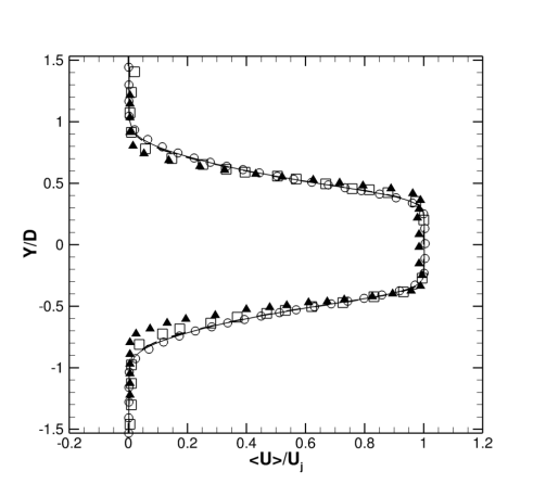
(a) $\langle U\rangle$ - X=2.5D ; $-1.5D\leq Y\leq 1.5D$

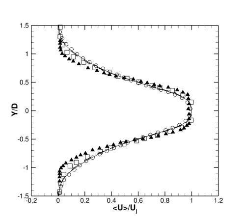
(b) $\langle U\rangle$ - X=5.0D ; $-1.5D\leq Y\leq 1.5D$

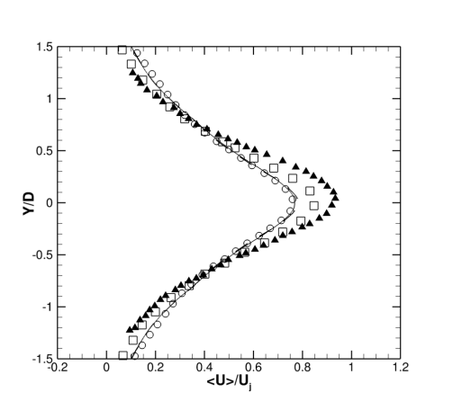
(c) $\langle U\rangle$ - X=10D ; $-1.5D\leq Y\leq 1.5D$

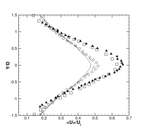
(d) $\langle U\rangle$ - X=15D ; $-1.5D\leq Y\leq 1.5D$

Figure 19: Profiles of averaged axial component of velocity at different positions within the computational domain. (–), S2 simulation; (–), S3 simulation; ($\bigcirc$), S4 simulation; ($\square$), numerical data; ($\blacktriangle$), experimental data.

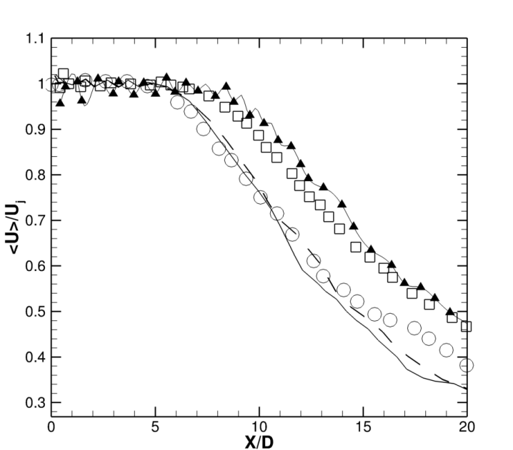
Figure 20: Evolution of the averaged axial component of velocity, $\langle U\rangle$, along the centerline (Y=0); (–), S2 simulation; (–), S3 simulation; ($\bigcirc$), S4 simulation; ($\square$), numerical data; ($\blacktriangle$), experimental data.

The four points at the lipline from the profiles presented in Figs. 19(a), 19(b), 19(c) and 19(d) are illustrated in Fig. 21 as an evolution the averaged axial component of velocity, $\langle U\rangle$, along the lipline. A spline is used to create the curve using the four points extracted from the $\langle U\rangle$ profiles at $X/D=2.5$, $X/D=5.0$, $X/D=10$ and $X/D=15$. The black line stands for the numerical data, the red line for the experimental, the green line for the S2 simulation, the red line for the S3 simulation and orange for the S4 simulation.

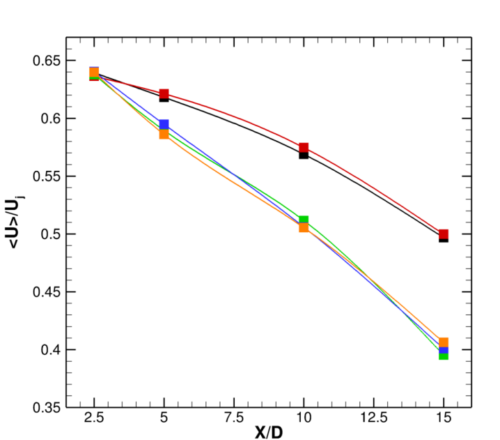
Figure 21: Extractions of the averaged axial component of velocity, $\langle U\rangle$, along the lipline (Y/D=0.5); $0\leq X\leq 20D$. ($\blacksquare$) numerical data; ( $\blacksquare$) experimental data; ($\blacksquare$) S2 simulation. ($\blacksquare$) S3 simulation. ($\blacksquare$) S4 simulation.

The comparison of profiles indicates that distributions of $\langle U\rangle$ calculated on S2, S3 and S4 simulations correlates well with the references until $X=5.0D$. For $X>10.0D$ all SGS models understimate the magnitude of $\langle U\rangle$ at the $-0.5D<Y<0.5D$ region when the results are compared with the reference data. One can notice that the evolution of $\langle U\rangle$ along the centerline, calculated by all three simulations, are in good agreement with the numerical and experimental reference data at the region where the mesh presents a good resolution. Moreover, the three distributions calculated using different SGS closures have presented a very similar behavior. Results from S2, S3 and S4 simulations along the lipline, presented in Fig. 21, also indicates a good correlation with the references data in the region where the mesh is more refined. The difference of magnitude of $\langle U\rangle$ at the lipline is about $20\%$ at $X=15.0D$.

8.6.2 Root Mean Square Distribution of Time Fluctuations of Axial Velocity Component

A lateral view of $u^{*}_{RMS}$ computed by S2, S3 and S4 simulations are presented in Figs. 22(a), 22(b) and 22(c), respectively.

(a) Lateral view of $u^{*}_{RMS}$ for S2 simulation.

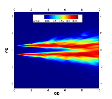
(b) Lateral view of $u^{*}_{RMS}$ for S3 simulation.

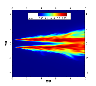
(c) Lateral view of $u^{*}_{RMS}$ for S4 simulation.

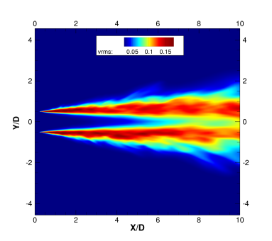
(d) Lateral view of $v^{*}_{RMS}$ for S2 simulation.

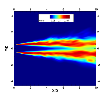
(e) Lateral view of $v^{*}_{RMS}$ for S3 simulation.

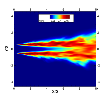
(f) Lateral view of $v^{*}_{RMS}$ for S4 simulation.

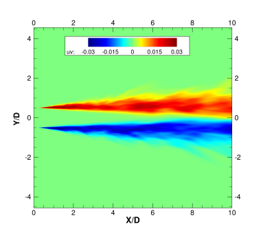
(g) Lateral view of $\langle u^{*}v^{*}\rangle$ for S2 simulation.

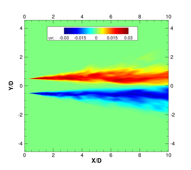
(h) Lateral view of $\langle u^{*}v^{*}\rangle$ for S3 simulation.

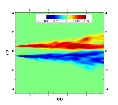
(i) Lateral view of $\langle u^{*}v^{*}\rangle$ for S4 simulation.

Figure 22: Lateral view of RMS of time fluctuation of axial component of velocity, $u_{RMS}^{*}$, RMS of time fluctuation of radial component of velocity, $v_{RMS}^{*}$ and $\langle u^{*}v^{*}\rangle$ Reynolds shear stress tensor component, for S2, S3 and S4 simulations.

The profiles of $u^{*}_{RMS}$ at $X=2.5D$ obtained by S2, S3 and S4 simulations are in good agreement with the numerical reference until $X=5.0D$, as one can observe in Fig. 23. For $X>10D$ the results achieved using the more refined mesh overestimate the magnitude of $u^{*}_{RMS}$ in the region where $-0.5D<Y<0.5D$. One should notice that all simulations, including the LES reference, present difficulties to predict the peaks of $u^{*}_{RMS}$.

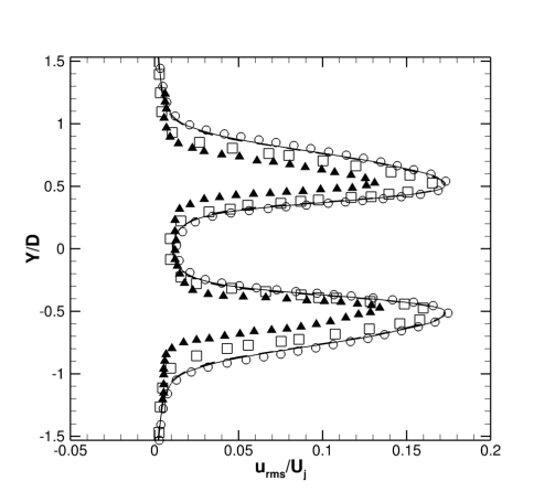
(a) $u^{*}_{RMS}$ - X=2.5D ; $-1.5D\leq Y\leq 1.5D$

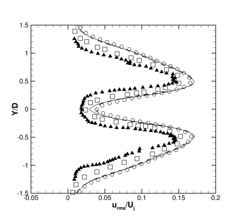
(b) $u^{*}_{RMS}$ - X=5.0D ; $-1.5D\leq Y\leq 1.5D$

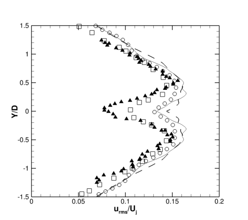
(c) $u^{*}_{RMS}$ - X=10D ; $-1.5D\leq Y\leq 1.5D$

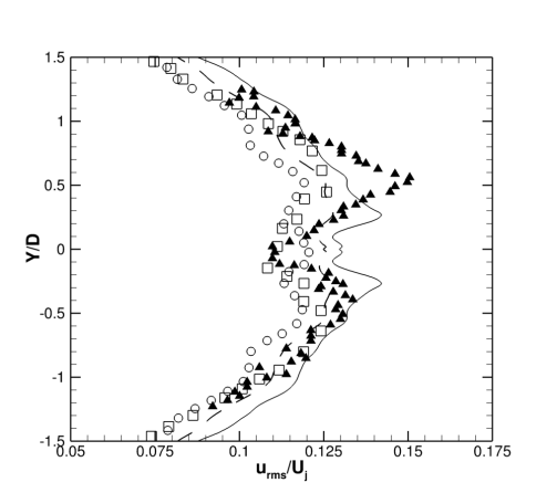
(d) $u^{*}_{RMS}$ - X=15D ; $-1.5D\leq Y\leq 1.5D$

Figure 23: Profiles of RMS of time fluctuation of axial component of velocity, $u_{RMS}^{*}$, for S2, S3 and S4, at different positions within the computational domain. (–), S2; (–), S3; ($\bigcirc$), S4; ($\square$), numerical data; ($\blacktriangle$), experimental data.

Figure 24 presents the distribution of $u_{RMS}^{*}$ along the centerline of the domain. All three simulations performed in the current work present overestimated distributions of $u_{RMS}^{*}$ along the centerline. However, for $10D<X<15D$, the Vreman model correctly reproduces the magnitude of $u_{RMS}^{*}$.

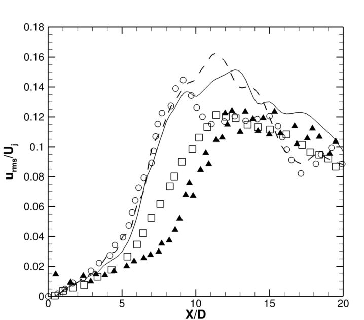
Figure 24: Evolution of RMS values of time fluctuation of axial component of velocity, $u_{RMS}^{*}$, along the centerline (Y=0); (–), S2; (–), S3; ($\bigcirc$), S4; ($\square$), numerical data; ($\blacktriangle$), experimental data.

The same strategy used in Fig. 21 is used to evaluate the magnitude of $u_{RMS}^{*}$ at four different points along the centerline. Figure 25 presents the points are extracted from Figs. 19(a), 19(b), 19(c) and 19(d). A spline is used to create the curve using the four points extracted from the $u_{RMS}^{*}$ at $X/D=2.5$, $X/D=5.0$, $X/D=10$ and $X/D=15$. The black line stands for the numerical data, the red line for the experimental, the green line for the S2 simulation, the blue line for the S3 simulation and orange for the S4 simulation. All numerical simulations, including the numerical reference, overpredict the fluctuations of $u_{RMS}^{*}$ at the lipline for $X=2.5D$ and $X=5.0D$. The Vreman model is the SGS model which presents better results of the peak of $u_{RMS}^{*}$ at the lipline for $X=10.0D$ when compared with the experimental reference. At $X=15.0D$ the dynamic Smagorinsky model presents the best prediction of the fluctuation of the axial velocity component at the the lipline. However, the other turbulent models present results which differ about $10\%$ from experimental data at the same point. The three SGS models provide similiar behavior of $u_{RMS}^{*}$ at the lipline region.

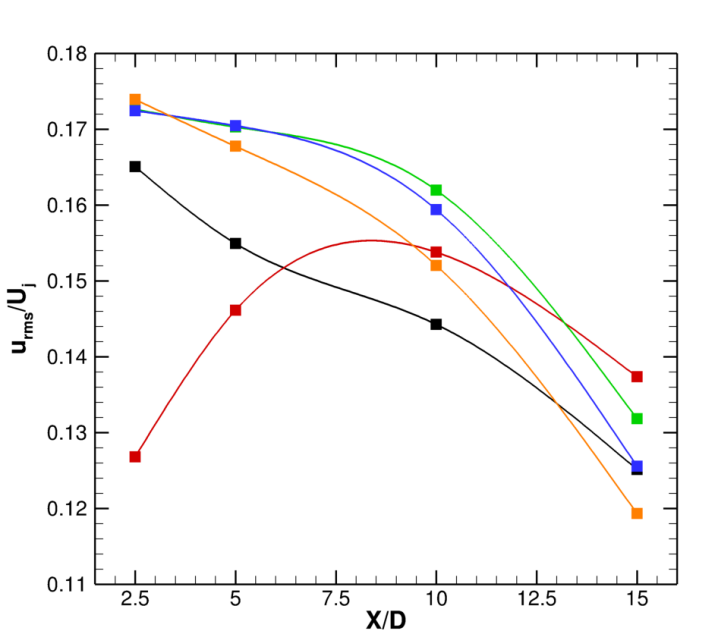
Figure 25: Extractions of RMS values of time fluctuation of axial component of velocity, $u_{RMS}^{*}$, along the lipline (Y/D=0.5); $0\leq X\leq 20D$. ($\blacksquare$) numerical data; ( $\blacksquare$) experimental data; ($\blacksquare$) S2 simulation. ($\blacksquare$) S3 simulation. ($\blacksquare$) S4 simulation.

8.6.3 Root Mean Square Distribution of Time Fluctuations of Radial Velocity Component

Effects of SGS modeling on the time fluctuation of the radial component of velocity are also compared with the reference data. Figures 22(d), 22(e) and 22(f) illustrate a lateral view of the distribution of $v_{RMS}^{*}$ computed by S2, S3 and S4 simulations, respectively. The choice of SGS model does not significantly affect the distribution of $v_{RMS}^{*}$. All distributions calculated by S2, S3 and S4 simulations have shown similar behavior.

Four profiles of $v_{RMS}^{*}$ at $X=2.5D$, $X=5.0D$, $X=10.0D$ and $X=15.0D$ are presented in Fig.  26. One can observe that all the profiles calculated on S2, S3 and S4 simulations are close to the reference at $X=2.5D$. The results correlates better with the experimental data than the numerical reference does at $X=2.5D$. The profile of $v_{RMS}^{*}$ calculated by S2, S3 and S4 at $X=5.0D$ are close to the experimental results. However, The numerical reference and the simulations performed in the present work, using the more refined mesh, present difficulties to predict the peaks of $v_{RMS}^{*}$ at the lipline region. For $X\geq 10.0D$ the S2, S3 and S4 computations fails to represent the profiles of $v_{RMS}^{*}$. The results are fairly underpredicted when comprared with the reference results due to the mesh coarsening.

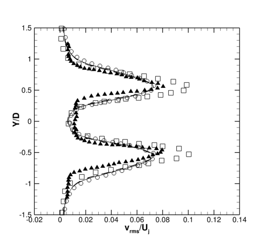
(a) $v^{*}_{RMS}$ - X=2.5D ; $-1.5D\leq Y\leq 1.5D$

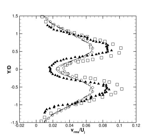
(b) $v^{*}_{RMS}$ - X=5.0D ; $-1.5D\leq Y\leq 1.5D$

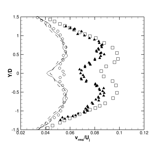
(c) $v^{*}_{RMS}$ - X=10D ; $-1.5D\leq Y\leq 1.5D$

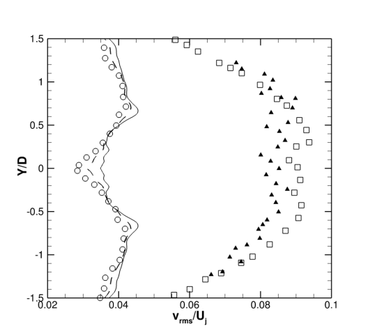
(d) $v^{*}_{RMS}$ - X=15D ; $-1.5D\leq Y\leq 1.5D$

Figure 26: Profiles of RMS of time fluctuation of radial component of velocity, $v_{RMS}^{*}$, for S1 and S2 simulations, at different positions within the computational domain. (–), simulation S2; (–), simulation S3; ($\bigcirc$), simulation S4; ($\square$), numerical data; ($\blacktriangle$), experimental data.

8.6.4 Component of Reynolds Stress Tensor

Figures 22(g), 22(h) and 22(i) present lateral view and profiles of $\langle u^{*}v^{*}\rangle$ component of the Reynolds stress tensor computed using three different SGS models, respectively. One can observe that the simulation performed using different SGS models have produced very similar distributions of $\langle u^{*}v^{*}\rangle$. All numerical simulations performed in the present work have difficulties to correctly predict the profiles of $\langle u^{*}v^{*}\rangle$ as presented in Fig.  27. At $X=2.5D$, S2, S3 and S4 calculations present a profile of $\langle u^{*}v^{*}\rangle$ which is similar to the reference data. However, the simulations performed in the current work fail to correctly represent the peaks near the lipline regions. For $X\geq 5.0D$ the $\langle u^{*}v^{*}\rangle$ profiles calculated in the present work fails to reproduce the shape and peaks of $\langle u^{*}v^{*}\rangle$. The cause of the issue could be related to an eventual lack of grid points in the radial direction. In spite of that, more studies on the subject are necessary in order to understand such behavior.

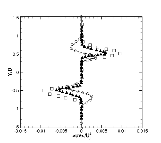
(a) $\langle u^{*}v^{*}\rangle$ - X=2.5D ; $-1.5D\leq Y\leq 1.5D$

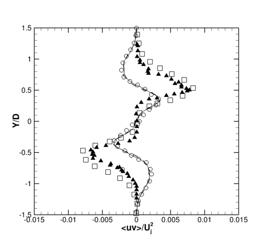
(b) $\langle u^{*}v^{*}\rangle$ - X=5.0D ; $-1.5D\leq Y\leq 1.5D$

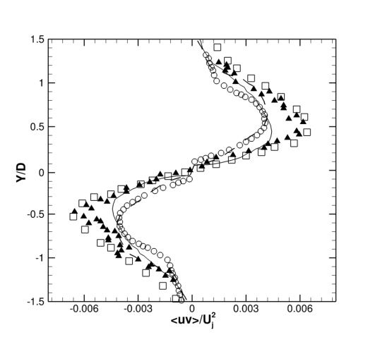
(c) $\langle u^{*}v^{*}\rangle$ - X=10D ; $-1.5D\leq Y\leq 1.5D$

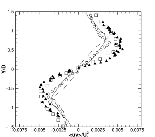
(d) $\langle u^{*}v^{*}\rangle$ - X=15D ; $-1.5D\leq Y\leq 1.5D$

Figure 27: Profiles of the $\langle u^{*}v^{*}\rangle$ Reynolds shear stress tensor component, for S2, S3 and S4 simulations, at different positions within the computational domain. (–), S2 simulation; (–), S3 simulation; ($\bigcirc$), S4 simulation; ($\square$), numerical data; ($\blacktriangle$), experimental data.

8.6.5 Time Averaged Eddy Viscosity

The distribution of the eddy viscosity, $\mu_{t}$, is discussed in the current subsection. Figure 28 presents distributions of time averaged eddy viscosity calculated using different SGS models. All subgrid scale closures used in the present work, the static Smagorinsky Smagorinsky [1963], Lilly [1965, 1967], the dynamic Smagorinsky Germano et al. [1991], Moin et al. [1991] and the Vreman Vreman [2004] models, are dependent of the local mesh size by design. This characteristic is exposed on the lateral view of the flow presented in Fig. 28. The SGS models are only acting in the region where mesh presents a low resolution. Near the entrance domain, where the computational grid is very refined, the eddy viscosity can be neglected.

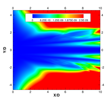
(a) $\langle\mu_{t}\rangle$ - S2 simulation

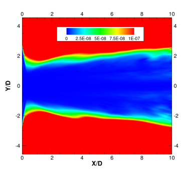
(b) $\langle\mu_{t}\rangle$ - S3 simulation

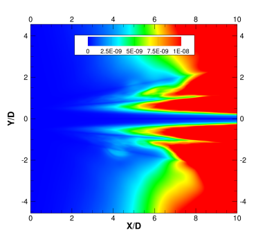
(c) $\langle\mu_{t}\rangle$ - S4 simulation

Figure 28: Lateral view of time averaged eddy viscosity, $\langle\mu_{t}\rangle$, for S2, S3 and S4 simulations.

The remark goes in the same direction of the work of Li and Wang Li and Wang [2015], which indicates that SGS closures introduce numerical dissipation that can be used as a stabilizing mechanism. However, this numerical dissipation does not necessarily add more physics of the turbulent flow to the LES solution. Therefore, in the present work, the numerical truncation, which generates the dissipative characteristic of JAZzY solutions, has shown to overcome the effects of the SGS modeling. The mesh needs to be very fine in order to achieve good results with second order spatial discretizations. The grid refinement generates very small grid spacing. Consequently, the SGS models, which are strongly dependent on the filter width, cannot have a very decisive effect on the solution. LES of compressible flow configurations without the use of SGS closures would be welcome in order to complete such discussion.

9 Concluding Remarks

The current work is concerned with a study of the effects of different subgrid scales models on perfectly expanded supersonic jet flow configurations using centered second-order spatial discretizations. A formulation based on the System I set of equations is used in the present work. The time integration is performed using a five-stage, second-order, explicit Runge-Kutta scheme. Four large eddy simulations of compressible jet flows are performed in the present research using two different mesh configurations and three different subgrid scale models. Their effects on the large eddy simulation solution are compared and discussed.

Large eddy simulations of high Reynolds supersonic jet flows using a second-order spatial discretization require high mesh resolution. A special care is necessary at the shear-layer region of the the jet flow. The mesh refinement study performed in the current study has indicated that, in the region where the grid presents high resolution, the simulations are in good agreement with experimental and numerical references. For the mesh with 14 million points, the simulation has produced good results for $X<2.5D$ For the other mesh, with 50 million points, the simulations provided good agreement with the literature for $X<5.0D$. The eddy viscosity, calculated by the static Smagorinsky model, presents very low levels in the region where the current results have good correlation with the data from the literature.

The refined grid used on the mesh refinement study, Mesh B, is selected for the comparison of SGS model effects on the results of the large eddy simulations. Three compressible jet flow simulations are performed using the classic Smagorinsky model Lilly [1967, 1965], Smagorinsky [1963], the dynamic Smagorinsky model Germano et al. [1991], Moin et al. [1991] and the Vreman model Vreman [2004]. All three simulations present similar behavior. Results yield good agreement with the references for $X<5.0D$. In the region where the grid is very fine and the results correlate well with the literature, the eddy viscosity coefficient, provided by the SGS model, has very low values. The reason for this behavior is related to the fact that the SGS closures used in the current work are strongly dependent on the filter width, which is proportional to the local mesh size.

The numerical results indicate that it is possible to achieve good results using second-order spatial discretizations for LES calculations. However, the mesh ought to be well resolved in order to overcome the truncation errors from the low order numerical scheme. Moreover, the numerical discretization can add significant artificial dissipation to the solution in the region where the mesh refinement is not well resolved. One can see this effect as a reduction of the local Reynolds number in the region where the mesh is not well refined which can be interpreted as a local overestimation of viscous effects in the flow.

It also of most importance the highlight here that very fine meshes yield very small filter widths. Consequently, the effects of the eddy viscosity coefficient calculated by the SGS models on the solution become unimportant for the numerical approach used in the current work. The work of Li and Wang Li and Wang [2015] have presented similar conclusions for simplified problems. Li and Wang further emphasize that SGS closures introduce numerical dissipation that can be used as a numerical stabilizing mechanism. However, this numerical dissipation does not necessarily add more physics of the turbulent flow behavior to the LES solution.

References

- ANSYS [2016] ANSYS. http://www.ansys.com/, 2016.
- Bigarella [2002] E. D. V. Bigarella. Three-dimensional turbulent flow over aerospace configurations. M.Sc. Thesis, Instituto Tecnológico de Aeronáutica, São José dos Campos, SP, Brasil, 2002.
- Bigarella [2007] E. D. V. Bigarella. Advanced Turbulence Modeling for Complex Aerospace Applications. PhD thesis, Instituto Tecnológico de Aeronáutica, São José dos Campos, SP, Brasil, 2007.
- Bridges and Wernet [2008] J. Bridges and M. P. Wernet. Turbulence associated with broadband shock noise in hot jets. In AIAA Paper No. 2008-2834, 14th AIAA/CEAS Aeroacoustics Conference, Vancouver, Canada, May 2008.
- Choi and Moin [2012] H. Choi and P. Moin. Grid-point requirements for large eddy simulation: Chapman’s estimates revisited. Physics of Fluids, 24(1):011702, Jan. 2012.
- Clark et al. [1979] R. A. Clark, J. Z. Ferziger, and W. C. Reynolds. Evaluation of subgrid-scale models using an accurately simulated turbulent flow. Journal of Fluid Mechanics, 91:1–16, 1979. doi: 0022-1 120/79/4207-6000.
- Deardorff [1970] J. W. Deardorff. A numerical study of three-dimensional turbulent channel flow at large reynolds numbers. Journal of Fluid Mechanics, 41, part 2:453–480, 1970.
- Garnier et al. [2009] E. Garnier, N. Adams, and P. Sagaut. Large Eddy Simulation for Compressible Flows. Springer, 2009. doi: 10.1007/978-90-481-2819-8.
- Germano [1990] M. Germano. Averaging invariance of the turbulent equations and similar subgrid scale modeling. In Center for Turbulence Research Manuscript 116. Stanford University and NASA - Ames Research Center, 1990.
- Germano et al. [1991] M. Germano, U. Piomelli, P. Moin, and W. H. Cabot. A dynamic subgridscale eddy viscosity model. Physics of Fluids A: Fluid Dynamics, 3(7), July 1991. doi: 10.1063/1.857955.
- Jameson and Mavriplis [1986] A. Jameson and D. Mavriplis. Finite volume solution of the two-dimensional euler equations on a regular triangular mesh. AIAA Journal, 24(4):611–618, Apr. 1986.
- Jameson et al. [1981] A. Jameson, W. Schmidt, and E. Turkel. Numerical solutions of the euler equations by finite volume methods using runge-kutta time-stepping schemes. In AIAA Paper 81–1259, Proceedings of the AIAA 14th Fluid and Plasma Dynamic Conference, Palo Alto, Californa, USA, June 1981.
- Junqueira-Junior [2016] C. Junqueira-Junior. Development of a Parallel Solver for Large Eddy Simulation of Supersonic Jet Flow. PhD thesis, Instituto Tecnológico de Aeronáutica, São José dos Campos, SP, Brazil, 2016.
- Junqueira-Junior et al. [2015] C. Junqueira-Junior, S. Yamouni, J. L. F. Azevedo, and W. R. Wolf. Large eddy simulations of supersonic jet flows for aeroacoustic applications. In AIAA Paper No. 2015-3306, Proceedings of the 33rd AIAA Applied Aerodynamics Conference, Dallas, TX, June 2015.
- Junqueira-Junior et al. [2016] C. Junqueira-Junior, S. Yamouni, J. L. F. Azevedo, and W. R. Wolf. Influence of Different Subgrid Scale Models in LES of Supersonic Jet Flows. In AIAA Paper No. 2016-4093, 46th AIAA Fuid Dynamics Conference, AIAA Aviation Forum, Washington, D.C., Jun. 2016.
- Leonard [1974] A. Leonard. Energy Cascade in Large Eddy Simulations of Turbulent Fluid Flows. Adv. Geophys., A18:237–48, 1974.
- Li and Wang [2015] Y. Li and Z. J. Wang. A priori and a posteriori evaluation of subgrid stress models with the Burger’s equation. In AIAA Paper No. 2015-1283, Proceedings of 53rd AIAA Aerospace Sciences Meeting, Kissimmee, FL, Jan. 2015.
- Lilly [1965] D. K. Lilly. On the computational stability of numerical solutions of time- dependent non-linear geophysical fluid dynamics problems. Monthly Weather Review, 93(1):11–25, January 1965. doi: 10.1175/1520-0493(1965)093¡0011:OTCSON¿2.3.CO;2.
- Lilly [1967] D. K. Lilly. The representation of small-scale turbulence in numerical simulation experiments. In IBM Form No. 320-1951, Proceedings of the IBM Scientific Computing Symposium on Environmental Sciences, pages 195–210, Yorktown Heights, N.Y., 1967.
- Long et al. [1991] L. N. Long, M. Khan, and H. T. Sharp. A Massively Parallel Three-Dimensional Euler/Navier-Stokes Method. AIAA Journal, 29(5):657–666, 1991.
- Mendez et al. [2010] S. Mendez, M. Shoeybi, A. Sharma, F. E. Ham, S. K. Lele, and P. Moin. Large-eddy simulations of perfectly-expanded supersonic jets: Quality assessment and validation. In AIAA Paper No. 2010–0271, 48th AIAA Aerospace Sciences Meeting Including the New Horizons Forum and Aerospace Exposition, Aerospace Sciences Meetings, Jan. 2010. doi: 10.2514/6.2010-271.
- Mendez et al. [2012] S. Mendez, M. Shoeybi, A. Sharma, F. E. Ham, and S. K. L. P. Moin. Large-eddy simulations of perfectly-expanded supersonic jets using an unstructured solver. AIAA Journal, 50(5):1103–1118, May 2012.
- Moin et al. [1991] P. Moin, K. Squires, W. Cabot, and S. Lee. A dynamic subgrid-scale model for compressible turbulence and scalar transport. Physics of Fluids A: Fluid Dynamics (1989-1993), 3(11):2746–2757, 1991. doi: 10.1063/1.858164.
- Sagaut [2002] P. Sagaut. Large Eddy Simulation for Incompressible Flows. Springer, 2002.
- Smagorinsky [1963] J. Smagorinsky. General circulation experiments with the primitive equations: I. the basic experiment. Monthly Weather Review, 91(3):99–164, March 1963. doi: 10.1175/1520-0493(1963)091¡0099:GCEWTP¿2.3.CO;2.
- Turkel and Vatsa [1994] E. Turkel and V. N. Vatsa. Effect of Artificial Viscosity on Three-Dimensional Flow Solutions. AIAA Journal, 32(1):39–45, 1994. URL http://doi.aiaa.org/10.2514/3.11948.
- Vreman [1995] A. W. Vreman. Direct and Large-Eddy Simulation of the Compressible Turbulent Mixing Layer. PhD thesis, Universiteit Twente, The Netherlands, 1995.
- Vreman [2004] A. W. Vreman. An eddy-viscosity subgrid-scale model for turbulent shear flow: Algebraic theory and applications. Physics of Fluids, 16(10), October 2004.
- Vreman et al. [1996] B. Vreman, B. Geurts, and H. Kuerten. Large-eddy simulation of the turbulent mixing layer using the Clark model. Theoretical Computational Fluid Dynamics, 8(4):309–324, 1996.
- Wang [2015] Z. J. Wang. Large eddy simulations of turbulent flows using discontinuous high order methods. In 22nd AIAA Computational Fluid Dynamics Conference, Invited talk, Dallas, TX, June 2015.
- Wolf et al. [2012] W. R. Wolf, J. L. F. Azevedo, and S. K. Lele. Convective effects and the role of quadrupole sources for aerofoil aeroacoustics. Journal of Fluid Mechanics, 708:502–538, 2012.
- Yoshizawa [1986] A. Yoshizawa. Statistical theory for compressible turbulent shear flows, with the application to subgrid modeling. Physics of Fluids, 29(7), July 1986. doi: 10.1063/1.865552.