From Hubble to Snap Parameters: A Gaussian Process Reconstruction

Abstract

By using recent $H(z)$ and SNe Ia data, we reconstruct the evolution of kinematic parameters $H(z)$, $q(z)$, jerk and snap, using a model-independent, non-parametric method, namely, the Gaussian Processes. Throughout the present analysis, we have allowed for a spatial curvature prior, based on Planck 18 Planck18 constraints. In the case of SNe Ia, we modify a python package (GaPP) SeikelEtAl12a in order to obtain the reconstruction of the fourth derivative of a function, thereby allowing us to obtain the snap from comoving distances. Furthermore, using a method of importance sampling, we combine $H(z)$ and SNe Ia reconstructions in order to find joint constraints for the kinematic parameters. We find for the current values of the parameters: $H_{0}=67.2\pm 6.2$ km/s/Mpc, $q_{0}=-0.60^{+0.21}_{-0.18}$, $j_{0}=0.90^{+0.75}_{-0.65}$, $s_{0}=-0.57^{+0.52}_{-0.31}$ at 1$\sigma$ c.l. We find that these reconstructions are compatible with the predictions from flat $\Lambda$CDM model, at least for 2$\sigma$ confidence intervals.

I Introduction

The relatively recent discovery of an accelerated expansion of the universe is confirmed by observations of Supernovae Type Ia (SNe Ia) pantheon and differential age of distant galaxies, through Hubble parameter ($H(z)$) measurements MaganaEtAl17 . It is well known that the standard model of cosmology, $\Lambda$CDM, fits quite well the observational data, however, alternative models have also been proposed recently to deal with some problems suffered by the standard model Bull2016 . Just to cite some examples of such alternative models, the dark energy and dark matter effects, or even the interaction among them, sometimes are inserted into the dynamic equations as new matter components GongBo ; marttens2020 ; SF ; Majerotto2009 ; Valiviita2010 ; Chimento2010 ; Cai2010 ; Sun2012 ; Pourtsidou2013 ; Salvatelli2014 ; Li2014 ; Skordis2015 ; Jimenez2016 ; Valent2020 .

Another way to study the cosmic evolution is through the so called cosmographic or kinematic models kine1 ; kine2 ; kine3 ; kine4 ; kine5 ; kine6 ; kine7 , where one is not worried about the Universe composition, but instead, how it evolves. In such models we seek for direct measures of expansion through its kinematic parameters (such as the Hubble parameter $H_{0}$, deceleration parameter $q$, jerk $j$ and snap $s$ parameters, etc). The main advantage of the method is to obtain a direct measure of expansion parameters directly from the data, with fewer assumptions than in dynamic modelling.

Recently, different types of cosmographic dark energy models have been studied. Running vacuum models has been studied in rezaei2021 , the study of cosmographic parameters in model independent approaches was done in mehrabi2021 , cosmographic functions up to the fourth order of derivative of the scale factor with the non-parametric method of Gaussian Processes was done in velasques2021 , among others.

One way to implement cosmographic modeling is to parameterize the cosmological parameters $H_{0}$, $q$, $j$ and $s$ for instance, or even higher orders if desired (crackle, pop, etc) lobo2020 . Another way is to obtain the cosmological parameters via reconstruction by Gaussian processes. Bilicki and Seikel Bilicki:2012 reconstructed $q(z)$, the normalized Hubble parameter ($E(z)$) and its two derivatives with respect to redshif $z$. Hai-Nan Lin et al NanLin:2019 reconstructed the normalized comoving distance $d_{C}(z)$, $E(z)$, $q(z)$ and the equation of state parameter $w(z)$. Ming-Jian Zhang and Jun-Qing Xia Zhang16 reconstructed $q(z)$ and the dimensionless comoving luminosity distance $D(z)$ (and its derivatives). Haridasu et al Haridasu18 reconstructed $q(z)$ and $E(z)$. Mukherjee and Banerjee reconstructed $q(z)$, $H(z)$, $D_{C}(z)$ (with two derivatives) Mukherjee20 and $j(z)$ Mukherjee21 .

The idea of Gaussian Processes (GP) is to obtain from a dataset $f(x_{i})\pm\sigma_{i}$ a reconstruction of the function $f(x)$. This is done by assuming that the errors in the data are Gaussian. In this way, the underlying function that describes the data is reconstructed as a Gaussian process, that is, it is generated from a point-to-point Gaussian distribution.

It is possible to show SeikelEtAl12a ; SeikelEtAl12b ; YuEtAl18 ; JesusEtAl20GP that the expected value $\mu$ and the variance $\sigma^{2}$ of the function $f(x)$ in the GP method are given by:

$$\mu(x) =\sum_{i,j=1}^{N}k(x,x_{i})(M^{-1})_{ij}f(x_{j})$$ (1)

$$\sigma^{2}(x) =k(x,x)-\sum_{i,j=1}^{N}k(x,x_{i})(M^{-1})_{ij}k(x_{j},x)$$ (2)

where $N$ is the number of data, the matrix $M_{ij}=k(x_{i},x_{j})+c_{ij}$, $c_{ij}$ is the covariance matrix of the data and $k(x,x^{\prime})$ is the covariance function or kernel between the points $x$ and $x^{\prime}$.

One of the main ingredients to obtain the GP reconstruction is the covariance function. As we assume that the data describe the same underlying $f(x)$ function, two points $x$ and $x^{\prime}$ are not independent of each other, so they have a covariance. To perform the reconstruction, it is necessary to choose a covariance function, the function that will model the correlation between these points. A commonly used covariance function is the quadratic exponential (or Gaussian) function:

$$k(x,x^{\prime})=\sigma_{f}^{2}\exp\left[-\frac{(x-x^{\prime})^{2}}{2l^{2}}\right]$$ (3)

where $\sigma_{f}$ and $l$ are hyperparameters of the covariance function. $\sigma_{f}$ is related to the vertical variation of the data and $l$ is related to the horizontal variation. In order to use the equations (1) and (2) to reconstruct the function $f(x)$, we need to determine the hyperparameters. They can be obtained from maximizing the logarithmic marginalized likelihood function:

$$\ln\mathcal{L}=-\frac{1}{2}\sum_{i,j=1}^{N}f(x_{i})\left(M^{-1}\right)_{ij}f(x_{j})-\frac{1}{2}\ln|M|-\frac{1}{2}N\ln 2\pi$$ (4)

where $|M|$ is the determinant of $M_{ij}$.

In this work we reconstruct the cosmological parameters $H(z)$, $q(z)$, $j(z)$ and $s(z)$ via the Gaussian Processes from SNe Ia data and $H(z)$ data. First we make the separate analysis for each set of data and then its combination.

The paper is organised as follows: In Section II we present the equations for the kinematic parameters. Section III contain the analyses and results and Section IV, the conclusions.

II Equations for kinematic parameters

The cosmological kinematic parameters are given by:

$$H =\frac{\dot{a}}{a}$$ (5)

$$q =-\frac{\ddot{a}}{aH^{2}}$$ (6)

$$j =\frac{\dddot{a}}{aH^{3}}$$ (7)

$$s =\frac{\ddddot{a}}{aH^{4}}$$ (8)

for Hubble, deceleration, jerk and snap parameters, respectively, where $a(t)$ is the scale factor of Friedmann-Robertson-Walker metric, $\dot{a}\equiv da/dt$ and $H=\dot{a}/a$. The negative sign on the deceleration parameter $q$ is due to historical reasons.

II.1 Kinematic Parameters from $H(z)$

The Gaussian Process (GP) will reconstruct $H(z)$ and its derivatives from $H(z)$ data and $D_{M}(z)$ from SNe Ia data. Let us then write the kinematic parameters in terms of $H(z)$ and its derivatives. First of all, let us realize that $\dot{a}=aH$ and $\frac{d}{dt}=-H(1+z)\frac{d}{dz}$. Thus:

$$q=-\frac{1}{aH^{2}}\frac{d(aH)}{dt}=\frac{H(1+z)}{aH^{2}}\frac{d(aH)}{dz}=\frac{(1+z)^{2}}{H}\frac{d}{dz}\left(\frac{H}{1+z}\right)=-1+(1+z)\frac{H^{\prime}(z)}{H(z)}$$ (9)

Let us now find an expression for the jerk. As shown in BenndorfEtAl22 , the jerk can be obtained from the deceleration parameter as

$$j(z)=(1+z)q^{\prime}(z)+q(1+2q)$$ (10)

Thus, from (9), we have

$$j(z)=1-2(1+z)\frac{H^{\prime}(z)}{H(z)}+(1+z)^{2}\frac{H^{\prime}(z)^{2}}{H(z)^{2}}+(1+z)^{2}\frac{H^{\prime\prime}(z)}{H(z)}$$ (11)

Finally, as shown in BenndorfEtAl22 , the snap can be obtained as

$$s(z)=-(1+z)j^{\prime}(z)-\left[2+3q(z)\right]j(z)$$ (12)

So, from Eqs. (9) and (11), we find

$$s(z)=1-3(1+z)\frac{H^{\prime}}{H}+3(1+z)^{2}\frac{H^{\prime 2}}{H^{2}}-(1+z)^{3}\frac{H^{\prime 3}}{H^{3}}-4(1+z)^{3}\frac{H^{\prime}H^{\prime\prime}}{H^{2}}+(1+z)^{2}\frac{H^{\prime\prime}}{H}-(1+z)^{3}\frac{H^{\prime\prime\prime}}{H}$$ (13)

where the primes denote derivatives with respect to the redshift $z$.

II.2 Kinematic Parameters from $D_{M}(z)$

In order to use the reconstruction made by the GPs for the SNe Ia data, let us write the kinematic parameters in terms of the dimensionless transverse comoving distance $D_{M}(z)$, which is given by

$$D_{M}(z)=\frac{1}{\sqrt{-\Omega_{k}}}\sin\left(\sqrt{-\Omega_{k}}D_{C}(z)\right)$$ (14)

where the line-of-sight comoving distance $D_{C}(z)$ relates to $E(z)\equiv\frac{H(z)}{H_{0}}$ as:

$$D_{C}^{\prime}(z)=\frac{1}{E(z)}\,,$$ (15)

where a prime denote a derivative with respect to redshift $z$. Dimensionless distances $D_{i}$ relate to dimensionful distances $d_{i}$ as:

$$D_{i}\equiv\frac{d_{i}}{d_{H}},$$ (16)

where $d_{H}\equiv\frac{c}{H_{0}}$ is Hubble distance.

The derivative with respect to $z$ of the transverse comoving distance $D_{M}(z)$ is

$$\dfrac{dD_{M}(z)}{dz}=D_{M}^{\prime}(z)=\cos\left(\sqrt{-\Omega_{k}}D_{C}(z)\right)D_{C}^{\prime}(z)\,,$$ (17)

so, by combining (14) and (17), we find:

$$\left(\frac{D_{M}^{\prime}}{D_{C}^{\prime}}\right)^{2}-\Omega_{k}D_{M}^{2}=1\,.$$ (18)

Now, by using (15), we can express the relation (18) in terms of the dimensionless quantity $E(z)$:

$$E^{2}=\frac{1+\Omega_{k}D_{M}^{2}}{D_{M}^{\prime 2}}\,.$$ (19)

Taking the derivative with respect to $z$ of the relation (19), we have

$$E\frac{dE}{dz}=\frac{\Omega_{k}D_{M}\left(D_{M}^{\prime 2}-D_{M}D_{M}^{\prime\prime}\right)-D_{M}^{\prime\prime}}{D_{M}^{\prime 3}}\,,$$ (20)

By dividing (20) by (19) and using (9), we find

$$q(z)=\frac{\Omega_{k}(1+z)D_{M}(z)D_{M}^{\prime}(z)}{1+\Omega_{k}D_{M}(z)^{2}}-(1+z)\frac{D_{M}^{\prime\prime}(z)}{D_{M}^{\prime}(z)}-1$$ (21)

Similarly, the jerk is given by

$$j(z)=1+\frac{\Omega_{k}(1+z)^{2}}{1+\Omega_{k}D_{M}^{2}}\left[D_{M}^{\prime 2}-\frac{2D_{M}D_{M}^{\prime}}{1+z}-3D_{M}D_{M}^{\prime\prime}\right]+\frac{(1+z)^{2}}{D_{M}^{\prime}}\left[\frac{3D_{M}^{\prime\prime 2}}{D_{M}^{\prime}}+\frac{2D_{M}^{\prime\prime}}{(1+z)}-D_{M}^{\prime\prime\prime}\right]$$ (22)

As we can see from these equations, one can always separate them in a part that depends on $\Omega_{k}$ and one that does not. Let us separate them in order to simplify equations. So, (21) can be written as:

$$q(z)=q_{f}(z)+q_{k}(z)$$ (23)

where

$$q_{f}(z) \equiv-1-(1+z)\frac{D_{M}^{\prime\prime}(z)}{D_{M}^{\prime}(z)}$$ (24)

$$q_{k}(z) \equiv\frac{\Omega_{k}(1+z)D_{M}(z)D_{M}^{\prime}(z)}{1+\Omega_{k}D_{M}(z)^{2}}$$ (25)

Similarly,

$$j(z)=j_{f}(z)+j_{k}(z)$$ (26)

where

$$j_{f}(z) \equiv 1+\frac{(1+z)^{2}}{D_{M}^{\prime}}\left[\frac{3D_{M}^{\prime\prime 2}}{D_{M}^{\prime}}+\frac{2D_{M}^{\prime\prime}}{(1+z)}-D_{M}^{\prime\prime\prime}\right]$$ (27)

$$j_{k}(z) \equiv\frac{\Omega_{k}(1+z)^{2}}{1+\Omega_{k}D_{M}^{2}}\left[D_{M}^{\prime 2}-\frac{2D_{M}D_{M}^{\prime}}{1+z}-3D_{M}D_{M}^{\prime\prime}\right]$$ (28)

Using (12), then, we have:

$$s(z)=-(1+z)j_{f}^{\prime}-(2+3q_{f})j_{f}-(1+z)j_{k}^{\prime}-(2+3q_{f}+3q_{k})j_{k}-3j_{f}q_{k}$$ (29)

From where we can identify:

$$s_{f}(z) \equiv-(1+z)j_{f}^{\prime}-(2+3q_{f})j_{f}$$ (30)

$$s_{k}(z) \equiv-(1+z)j_{k}^{\prime}-(2+3q_{f}+3q_{k})j_{k}-3j_{f}q_{k}$$ (31)

So:

$$s_{f}(z) =1+\frac{(1+z)^{3}D_{M}^{(4)}}{D_{M}^{\prime}}-\frac{(1+z)^{2}D_{M}^{(3)}}{D_{M}^{\prime}}+\frac{15(1+z)^{3}D_{M}^{\prime\prime 3}}{D_{M}^{\prime 3}}+$$

$$+\frac{5(1+z)^{2}D_{M}^{\prime\prime 2}}{D_{M}^{\prime 2}}+\frac{3(1+z)D_{M}^{\prime\prime}}{D_{M}^{\prime}}-\frac{10(1+z)^{3}D_{M}^{(3)}D_{M}^{\prime\prime}}{D_{M}^{\prime 2}}$$ (32)

$$s_{k}=\frac{\Omega_{k}(1+z)}{\left(1+\Omega_{k}D_{M}^{2}\right)^{2}D_{M}^{\prime}} \left\{\Omega_{k}(1+z)D_{M}^{2}D_{M}^{\prime 2}\left(7(1+z)D_{M}^{\prime\prime}+3D_{M}^{\prime}\right)+(1+z)D_{M}^{\prime 2}\left(4(1+z)D_{M}^{\prime\prime}+D_{M}^{\prime}\right)\right.+$$

$$-\Omega_{k}D_{M}^{3}\left[18(1+z)^{2}D_{M}^{\prime\prime 2}+3D_{M}^{\prime 2}+(1+z)D_{M}^{\prime}\left(7D_{M}^{\prime\prime}-6(1+z)D_{M}^{(3)}\right)\right]+$$

$$-D_{M}\left[18(1+z)^{2}D_{M}^{\prime\prime 2}+\Omega_{k}(1+z)^{2}D_{M}^{\prime 4}+3D_{M}^{\prime 2}\right.+$$

$$+(1+z)\left.D_{M}^{\prime}\left.\left(7D_{M}^{\prime\prime}-6(1+z)D_{M}^{(3)}\right)\right]\right\}\,.$$ (33)

With these expressions, we can reconstruct the kinematic parameters evolution from $H(z)$ and SNe Ia data.

III Analyses and Results

The observational data sample used in this work is formed by the $1048$ SNe Ia measurements from the Pantheon sample pantheon and a compilation of $32$ Hubble parameter data, $H(z)$ MorescoEtAl22 , obtained by estimating the differential ages of galaxies, called cosmic chronometers.

Concerning the Pantheon sample, we have followed the same idea as in JesusEtAl20GP and JesusEtAl22GP . As explained in JesusEtAl20GP , as the Pantheon sample consists of apparent magnitude SNe Ia data, this is not suitable for GP reconstruction, as magnitudes diverge for $z\rightarrow 0$ and GP fails to reconstruct rapidly varying functions as explained in SeikelEtAl12a . Thus, we made a error propagation from magnitudes to comoving distances, as explained in JesusEtAl20GP .

The 32 $H(z)$ Cosmic Chronometers (CCs) data is a sample compiled by MorescoEtAl22 , where they have, for the first time, estimated systematic errors for these data. In order to do that, they have made simulations and have considered effects as metallicity, rejuvenation effect, star formation history, initial mass function, choice of stellar library etc.

We have used the publicly available software GaPP by SeikelEtAl12a in order to make the reconstructions in the present work. It is important to mention, however, that the original software were able only to reconstruct function derivatives up to third order, while to obtain the snap reconstruction from SNe Ia, we need the fourth derivative of comoving distance, as can be seen in Eq. (32). We have then modified the original software in order to obtain fourth order function derivatives.

Using the GP method, we were able to reconstruct the Hubble parameter $H(z)$ from the cosmic chronometers data, and the $D_{M}(z)$ using the Pantheon sample data. These reconstructions are shown in Fig. 1, where the left figure corresponds to the plot of cosmic chronometers data together with the reconstruction of $H(z)$ and the right figure shows the reconstruction and the data of $D_{M}(z)$ obtained from the Pantheon sample.

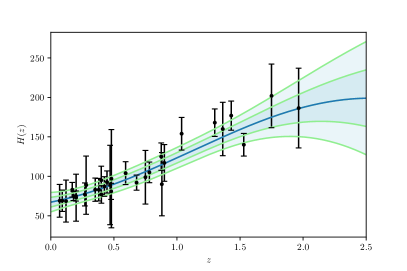
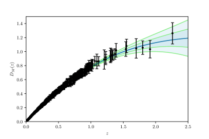
Figure 1: GP reconstructions from data. a) Left: Reconstruction of $H(z)$ (in km/s/Mpc) function from 32 $H(z)$ data with covariance. b) Right: Reconstruction of dimensionless $D_{M}(z)$ from Pantheon SNe Ia data.

In order to obtain the reconstruction of the kinematic parameters in terms of $D_{M}(z)$, using Eqs. (19), (21), (22) and (29), however, we need to get a free parameter, $\Omega_{k}$. This parameter is not obtained from the reconstruction, it must be constrained with the aid of other observations, which can provide a prior on $\Omega_{k}$.

The prior used was provided by Planck 18 (TT,TE,EE+lowE) Planck18 , where $\Omega_{k}=-0.044\pm 0.050,$ at 3$\sigma$ c.l. We chose to work with a 3$\sigma$ prior in order to allow for a more model-independent analysis. With this prior over $(\Omega_{k})$, we can obtain the kinematic parameters by sampling this prior and the multivariate Gaussian corresponding to $H(z)$, $D_{M}(z)$ and their derivatives.

We also performed the reconstruction of the kinematic parameters with the combination of $H(z)$ data and the Pantheon sample, in the redshift range where the respective reconstructions were compatible in $1\sigma$. This analysis was performed by weighting the reconstruction obtained for $D_{M}(z)$ with the reconstruction of $H(z)$, by a MCMC method known as importance sampling. It is the first time that such a combination of GP reconstructions is made in the literature, as far as we know.

For each reconstruction of kinematic parameter below, we also show the constraints obtained from Planck 18 (Plik,TT,TE,EE+lowE+lensing) Planck18 , for a flat $\Lambda$CDM model, corresponding to $\Omega_{m}=0.3153\pm 0.0073$, $H_{0}=67.36\pm 0.54$ km/s/Mpc. Although in the model-independent GP analysis we have chosen to allow for some spatial curvature, we chose to compare with the flat $\Lambda$CDM model, as this is regarded as the standard, cosmic concordance model. Concerning the $H_{0}$ tension, as Pantheon alone does not constrain $H_{0}$ and we intended to combine reconstructions from $H(z)$ and SNe Ia data, we do not reconstruct $H(z)$, but $E(z)$ instead, which is independent of $H_{0}$. In the end of the section, however, we compare the $H_{0}$ determinations from $H(z)$, Planck 18 and SH0ES.

III.1 $E(z)$ Reconstruction

The $E(z)$ reconstructions obtained by GP are shown with 1 and $2\sigma$ confidence intervals in Fig. 2.

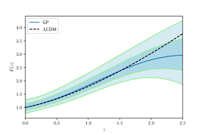
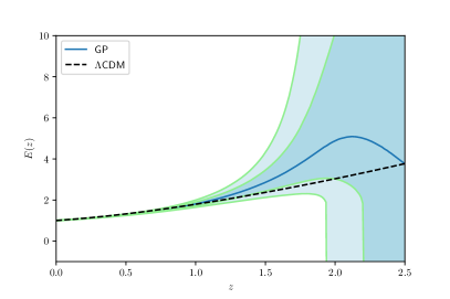
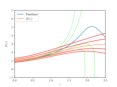
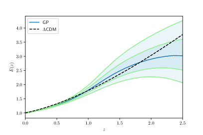
Figure 2: $E(z)$ reconstruction. a) Top Left: Reconstruction from $H(z)$ data. b) Top Right: Reconstruction from SNe Ia. c) Bottom Left: Comparison between reconstructions. d) Bottom Right: Joint reconstruction.

In Fig. 2, at the top left, we show the $E(z)$ reconstruction for the $H(z)$ data. The dashed line corresponds to $E(z)$ for the flat $\Lambda$CDM model, with $\Omega_{m}$ obtained from Planck 18. The $\Lambda$CDM model prediction is compatible within $1\sigma$ with the GP reconstruction for $z\lesssim 2.3$, being compatible within 2$\sigma$ in the remaining interval. The top right figure shows the reconstruction of $E(z)$ made with the Pantheon sample data. As we can see, the standard $\Lambda$CDM model is compatible with the GP reconstruction within $1\sigma$ for most part of the redshift interval, being compatible at $2\sigma$ only for an intermediate interval, $1.2\lesssim z\lesssim 1.9$.

In the bottom left figure, we show the superimposed reconstructions in order to see at which redshift interval they are compatible at 1$\sigma$, thus allowing us to safely make a joint analysis. We find that they are compatible within 1$\sigma$ for all the analyzed interval, $0<z<2.5$, thus we proceeded to the full joint analysis, which can be seen in the bottom right figure. As can be seen in Fig. 2d, only at $z\gtrsim 2.4$ the standard model is not compatible with GP joint analysis within 1$\sigma$, being compatible at 2$\sigma$, however.

III.2 $q(z)$ Reconstruction

In Fig. 3 we show the reconstruction of $q(z)$ with a confidence interval of $2\sigma$.

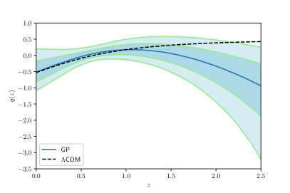
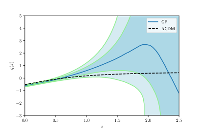
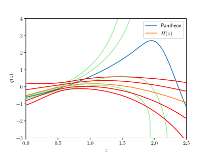
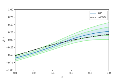
Figure 3: $q(z)$ reconstruction. a) Top Left: Reconstruction from $H(z)$ data. b) Top Right: Reconstruction from SNe Ia. c) Bottom Left: Comparison between reconstructions. d) Bottom Right: Joint reconstruction.

In Fig. 3a, we see the $q(z)$ reconstruction from CCs. As one can see, the $\Lambda$CDM model is compatible with the GP reconstruction within 2$\sigma$ for a large interval, up to $z\approx 2.3$. For the reconstruction from SNe Ia (Fig. 3b), however, the compatibility within 2$\sigma$ remains for the whole interval, $0\leq z\leq 2.5$.

In Fig. 3c, we superimpose both reconstructions in order to combine them. One may see that they are compatible within 1$\sigma$ for $z\lesssim 1.2$, so we made the joint analysis, which can be seen on Fig. 3d. As one may see, for this interval, the $\Lambda$CDM model prediction is within 2$\sigma$ c.l. from the joint reconstruction.

III.3 $j(z)$ Reconstruction

We show the reconstruction of $j(z)$ with $2\sigma$ uncertainty in Fig. 4.

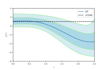
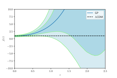
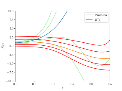
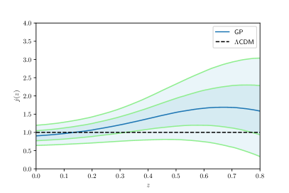
Figure 4: $j(z)$ reconstruction. a) Top Left: Reconstruction from $H(z)$ data. b) Top Right: Reconstruction from SNe Ia. c) Bottom Left: Comparison between reconstructions. d) Bottom Right: Joint reconstruction.

In Fig. 4a, we may see the jerk reconstruction from CCs. The comparison with the $\Lambda$CDM model here is quite interesting, as the standard, flat $\Lambda$CDM model predict a exact value $j(z)=1$. One may see from this Figure, that only at a high reshift interval, $1.9\lesssim z\lesssim 2.4$, $\Lambda$CDM is outside of the 2$\sigma$ interval of the GP reconstruction. For the SNe Ia reconstruction, however, one may see in Fig. 4b, that the $\Lambda$CDM model is within 2$\sigma$ for the whole redshift interval.

In Fig. 4c, we have superimposed both reconstructions. One may see that both reconstructions agree only for $z\lesssim 0.8$, so, in Fig. 4d, we made the combination of the reconstructions only in this interval. One may see that the $\Lambda$CDM model agrees with the joint reconstruction for all this redshift interval, within 2$\sigma$ c.l.

III.4 $s(z)$ Reconstruction

The reconstruction of $s(z)$ obtained with GP is shown in Fig. 5.

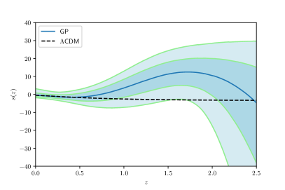
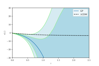
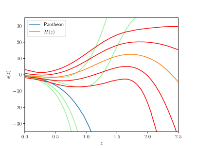
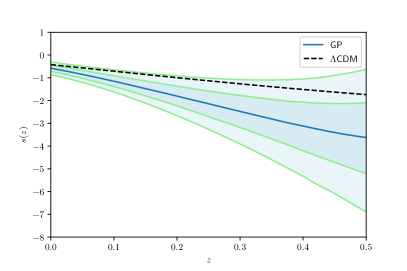
Figure 5: $s(z)$ reconstruction. a) Top Left: Reconstruction from $H(z)$ data. b) Top Right: Reconstruction from SNe Ia. c) Bottom Left: Comparison between reconstructions. d) Bottom Right: Joint reconstruction.

As can be seen on Figs. 5a and 5b, the $\Lambda$CDM model is compatible within 2$\sigma$ with both reconstructions. In Fig. 5c, one may see that both reconstructions agree within 1$\sigma$ only for a small interval, $z\lesssim 0.5$. The joint reconstruction in this interval can be seen on Fig. 5d, where can be seen that the $\Lambda$CDM model is compatible with it for this whole interval. The situation in this case, however, is interesting because in the whole interval the concordance model is compatible only at the 2$\sigma$ c.l.

III.5 Current values of kinematic parameters from Gaussian Processes

As one could see above, the kinematic parameters were better constrained at lower redshifts. So, in this subsection, we focus in the constraints for the current values of the kinematic parameters, which have great interest in the literature. In Table 1, we show the values of the kinematic parameters today in $z=0$, which we obtained through the GP reconstructions. We also show the constraints obtained from Planck 18 Planck18 for a flat $\Lambda$CDM model, corresponding to $\Omega_{m}=0.315\pm 0.007$. We have compatibility within $1\sigma$ c.l. for the $\Lambda$CDM model with our results. The value of $H_{0}$ that we obtain with GP is also compatible in $1\sigma$ with the value $H_{0}=73.2\pm 1.7\pm 2.4$ km/s/Mpc found by SH0ES Riess:2016jrr .

We should also compare these values with the ones obtained of kinematic parametrizations in BenndorfEtAl22 . In their best parametrization, $j(z)=j_{0}$, they have obtained $H_{0}=68.8\pm 1.9$ km/s/Mpc, $q_{0}=-0.578\pm 0.067$, $j_{0}=1.15\pm 0.28$ and $s_{0}=-0.255^{+0.094}_{-0.21}$ at 1$\sigma$ c.l. This result is from Pantheon+31 $H(z)$ data from MaganaEtAl17 , without systematics. We may see that this is compatible within 1$\sigma$ with our results in Table 1. However, while the $H_{0}$ value was compatible with SH0ES only at 2$\sigma$ c.l., we now have compatibility with SH0ES at 1$\sigma$ c.l. thanks to taking the systematics into account.

Parameter	Gaussian Processes Reconstruction			$\Lambda$CDM Model
	$H(z)$	SNe Ia	Joint	Planck 18
$H_{0}$ (km/s/Mpc)	$67.2\pm 6.15\pm 12.3$			$67.4\pm 0.5\pm 1.0$
$q(z=0)$	$-0.51^{+0.34+0.72}_{-0.30-0.56}$	$-0.61^{+0.05+0.10}_{-0.05-0.10}$	$-0.60^{+0.21+0.45}_{-0.18-0.35}$	$-0.528\pm 0.011\pm 0.021$
$j(z=0)$	$1.1^{+0.81+1.7}_{-0.71-1.3}$	$0.90^{+0.14+0.29}_{-0.13-0.26}$	$0.90^{+0.75+1.56}_{-0.65-1.2}$	$1$
$s(z=0)$	$-0.43^{+1.2+3.6}_{-0.71-1.4}$	$-0.58^{+0.13+0.26}_{-0.13-0.26}$	$-0.57^{+0.52+1.56}_{-0.31-0.62}$	$-0.418\pm 0.032\pm 0.064$

Table 1: Current values of kinematic parameters ($z=0$), obtained with GP.

In Fig. 6, we show the joint distributions found for the current values of the kinematic parameters $q_{0}$, $j_{0}$ and $s_{0}$. We do not show the $H_{0}$ distribution here because it comes only from $H(z)$ data and it is a Normal distribution as expected from Gaussian Processes.

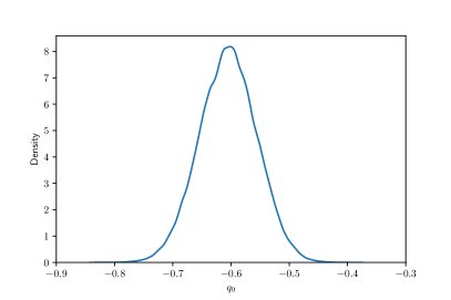
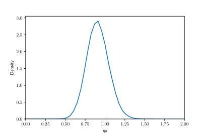
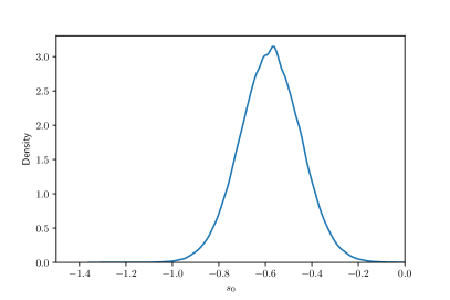
Figure 6: Current values of the kinematic parameters from the GP joint reconstructions.

IV Conclusions

We have reconstructed the evolution of four kinematic parameters, namely, $E(z)$, $q(z)$, $j(z)$ and $s(z)$, from Pantheon and $H(z)$ data. For the first time, we have used $H(z)$ data with systematical errors in this kind of analysis. In order to obtain model-independent reconstructions, we have allowed for a prior in the spatial curvature, coming from Planck 18 analysis. Differently from earlier analyses, $H_{0}$ obtained from $H(z)$ data is now compatible within 1$\sigma$ both with Planck 18 and SH0ES, thereby not favouring any of the poles of the $H_{0}$ tension. We have made a combination of the reconstructions in each case, for the redshift intervals where it was safe to make it. For all reconstructions, the so-called cosmic concordance flat $\Lambda$CDM model is compatible within 2$\sigma$ in the analyzed redshift intervals. A general tendency is that SNe Ia constrain better at lower redshifts, while $H(z)$ data constrain better at higher redshifts, thereby showing the importance of such a combination. Both reconstructions agree at lower redshifts and lower derivatives, while being less compatible at higher redshifts and derivatives.

Other possibilities, as including more data and reconstructing other kinematic parameters can be explored in a forthcoming issue.

- (1) N. Aghanim et al. [Planck], Astron. Astrophys. 641 (2020), A6 [erratum: Astron. Astrophys. 652 (2021), C4] [arXiv:1807.06209 [astro-ph.CO]].
- (2) M. Seikel, C. Clarkson, M. Smith, JCAP 06 (2012), 036 [arXiv:1204.2832 [astro-ph.CO]].
- (3) D. M. Scolnic et al., Astrophys. J. 859 (2018) no.2, 101 [arXiv:1710.00845 [astro-ph.CO]].
- (4) J. Magana, M. H. Amante, M. A. Garcia-Aspeitia and V. Motta, Mon. Not. Roy. Astron. Soc. 476 (2018) no.1, 1036-1049 [arXiv:1706.09848 [astro-ph.CO]].
- (5) P. Bull et al., Phys. the Dark Universe 12 (2016) 56 [arXiv:1512.05356 [astro-ph.CO]].
- (6) Gong-Bo Zhao et al., Nature Astronomy, 1, 627, (2017), [arXiv:1701.08165 [astro-ph.CO]].
- (7) R. von Marttens, L. Lombriser, M. Kunz, V. Marra, L. Casarini, J. Alcaniz, Phys. Dark Universe, 28, (2020), 100490, [arXiv:1911.02618 [astro-ph.CO]].
- (8) S.H. Pereira, J.F. Jesus, Phys.Rev.D 79 (2009) 043517, [arXiv:0811.0099 [astro-ph]].
- (9) E. Majerotto, J. Valiviita, R. Maartens, Mon.Not.Roy.Astron.Soc. 402 (2010) 2344, [arXiv:0907.4981 [astro-ph.CO]].
- (10) J. Valiviita, R. Maartens, E. Majerotto, Mon.Not.Roy.Astron.Soc. 402 (2010) 2355, [arXiv:0907.4987 [astro-ph.CO]].
- (11) L. P. Chimento, Phys.Rev.D 81 (2010) 043525, [arXiv:0911.5687 [astro-ph.CO]].
- (12) Rong-Gen Cai, Qiping Su, Phys.Rev.D 81 (2010) 103514, [arXiv:0912.1943 [astro-ph.CO]].
- (13) Cheng-Yi Sun, Rui-Hong Yue, Phys.Rev.D 85 (2012) 043010, [arXiv:1009.1214 [gr-qc]].
- (14) A. Pourtsidou, C. Skordis, E.J. Copeland, Phys.Rev.D 88 (2013) 8, 083505, [arXiv:1307.0458 [astro-ph.CO]].
- (15) V. Salvatelli, N. Said, M. Bruni, A. Melchiorri, D. Wands, Phys.Rev.Lett. 113 (2014) 18, 181301, [arXiv:1406.7297 [astro-ph.CO]].
- (16) Yun-He Li, Xin Zhang, Phys.Rev.D 89 (2014) 8, 083009, [arXiv:1312.6328 [astro-ph.CO]].
- (17) C. Skordis, A. Pourtsidou, E.J. Copeland, Phys.Rev.D 91 (2015) 8, 083537, [arXiv:1502.07297 [astro-ph.CO]].
- (18) J. B. Jiménez, D. Rubiera-Garcia, D. Sáez-Gómez, V. Salzano, Phys.Rev.D 94 (2016) 12, 123520, [arXiv:1607.06389 [gr-qc]].
- (19) A. Gómez-Valent, V. Pettorino and L. Amendola, Phys. Rev. D 101 (2020) no.12, 123513 [arXiv:2004.00610 [astro-ph.CO]].
- (20) M. Visser, Class. Quant. Grav. 21 (2004) 2603 [gr-qc/0309109].
- (21) M. Visser, Gen. Rel. Grav. 37 (2005) 1541 [gr-qc/0411131].
- (22) C. Shapiro and M. S. Turner, Astrophys. J. 649 (2006) 563 [astro-ph/0512586].
- (23) R. D. Blandford, M. A. Amin, E. A. Baltz, K. Mandel and P. J. Marshall, ASP Conf. Ser. 339 (2005) 27 [astro-ph/0408279].
- (24) Ø. Elgarøy and T. Multamäki, JCAP 0609 (2006) 002 [astro-ph/0603053].
- (25) D. Rapetti, S. W. Allen, M. A. Amin and R. D. Blandford, Mon. Not. Roy. Astron. Soc. 375 (2007) 1510 [astro-ph/0605683].
- (26) A. G. Riess et al., Astrophys. J. 659 (2007) 98 [astro-ph/0611572].
- (27) M. Rezaei, J. Solà Peracaula and M. Malekjani, Mon. Not. Roy. Astron. Soc. 509 (2021) no.2, 2593-2608 [arXiv:2108.06255 [astro-ph.CO]].
- (28) A. Mehrabi, M. Rezaei, Astrophys. J. 923 (2021) 2, 274, [2110.14950 [astro-ph.CO]].
- (29) A. M. Velasquez-Toribio and J. C. Fabris, Braz. J. Phys. 52 (2022) no.4, 115 [arXiv:2104.07356 [astro-ph.CO]].
- (30) F. S. N. Lobo, J. P. Mimoso, M. Visser, JCAP 04 (2020) 043, [2001.11964 [gr-qc]].
- (31) M. Bilicki, M. Seikel, Astronomical Society, Volume 425, Issue 3, September 2012, Pages 1664–1668,
- (32) H. Lin, X. Li, L. Tang, Chinese Physics C 43 (2019) 075101 [arXiv:1905.11593 [gr-qc]].
- (33) M. Zhang, J. Xia, JCAP 12 (2016), 005
- (34) B. S. Haridasu, V. V. Luković, M. Moresco, N. Vittorio, JCAP , 10 (2018), 015
- (35) P. Mukherjee, N. Banerjee, Physics of the Dark Universe 36 (2022), 100998 [arXiv:2007.15941 [astro-ph.CO]].
- (36) P. Mukherjee, N. Banerjee, The European Physical Journal C 81 (2021), 36 [arXiv:2007.10124 [astro-ph.CO]].
- (37) M. Seikel, S. Yahya, R. Maartens, C. Clarkson, Phys. Rev. D 86 (2012), 083001 [arXiv:1205.3431 [astro-ph.CO]].
- (38) H. Yu, B. Ratra, F. Wang, 2018 ApJ 856 3 [arXiv:1711.03437 [astro-ph.CO]].
- (39) J. F. Jesus, R. Valentim, A. A. Escobal, S. H. Pereira, JCAP 04 (2020), 053 [arXiv:1909.00090 [astro-ph.CO]].
- (40) D. Benndorf, J.F. Jesus and S.H. Pereira, Eur. Phys. J. C 82, 457 (2022).
- (41) M. Moresco, L. Amati, L. Amendola, S. Birrer, J. P. Blakeslee, M. Cantiello, A. Cimatti, J. Darling, M. Della Valle and M. Fishbach, et al. Living Rev. Rel. 25 (2022) no.1, 6 [arXiv:2201.07241 [astro-ph.CO]].
- (42) J. F. Jesus, R. Valentim, A. A. Escobal, S. H. Pereira and D. Benndorf, JCAP 11 (2022), 037 [arXiv:2112.09722 [astro-ph.CO]].
- (43) A. G. Riess et al. ‘A 2.4% Determination of the Local Value of the Hubble Constant,” Astrophys. J. 826 (2016) no.1, 56