A Cut-and-solve Algorithm for Virtual Machine Consolidation Problem

Abstract

The virtual machine consolidation problem (VMCP) attempts to determine which servers to be activated, how to allocate virtual machines (VMs) to the activated servers, and how to migrate VMs among servers such that the summation of activated, allocation, and migration costs is minimized subject to the resource constraints of the servers and other practical constraints. In this paper, we first propose a new mixed integer linear programming (MILP) formulation for the VMCP. We show that compared with existing formulations, the proposed formulation is much more compact in terms of smaller numbers of variables or constraints, which makes it suitable for solving large-scale problems. We then develop a cut-and-solve (C&S) algorithm, a tree search algorithm to efficiently solve the VMCP to optimality. The proposed C&S algorithm is based on a novel relaxation of the VMCP that provides a stronger lower bound than the natural continuous relaxation of the VMCP, making a smaller search tree. By extensive computational experiments, we show that (i) the proposed formulation significantly outperforms existing formulations in terms of solution efficiency; and (ii) compared with standard MILP solvers, the proposed C&S algorithm is much more efficient.

1 Introduction

Nowadays, cloud computing provides a great flexibility and availability of computing resources to customers and has become more and more popular in many industries including the manufacturing industry [1], conference management systems [2], and E-commerce [3]. The reason behind this success is that cloud service providers can provide customers with reliable, inexpensive, customized, and elastically priced computing resources without requiring customers to host them at a dedicated place. In particular, various applications requested by different customers can be instantiated inside virtual machines (VMs) and flexibly deployed to any server in any data center of the cloud [4]. However, as VMs change dynamically and run over a shared common cloud infrastructure, it is crucial to (re)allocate cloud resources (by migrating existing VMs among different servers and/or mapping new VMs into appropriate servers) to meet diverse application requirements while minimizing the operational costs of the service providers. The above problem is called the virtual machine consolidation problem (VMCP) in the literature, which determines the activation state of all servers and the (re)allocation of all VMs in such a way that the predefined cost function (server activation, VM allocation, and migration costs) is minimized subject to resource constraints of the servers and other practical constraints.

The VMCP is strongly NP-hard, as it includes the bin packing problem (BPP) [5]. Therefore, there is no polynomial-time algorithm to solve the VMCP to optimality unless P = NP. As a result, most existing works investigated heuristic algorithms for solving the VMCP. In particular, the first-fit decreasing and best-fit decreasing algorithms, first investigated for BPPs, are used to solve VMCPs; see [6, 5]. Reference [5] first formulated the VMCP as a mixed integer linear programming (MILP) problem and then proposed a linear programming (LP) relaxation based heuristic algorithm. This heuristic algorithm solves the LP relaxation of the MILP problem, fixes the variables taking integral values, and tries to find a solution by solving the reduced MILP problem. Reference [7] proposed a heuristic algorithm based on the convex optimization method and dynamic programming. Several metaheuristic algorithms were also developed to solve the VMCP, including genetic algorithm [8, 9, 10], simulated annealing [11], colony optimization [12, 13], and evolution algorithm [14]. However, the above heuristic algorithms cannot guarantee to find an optimal solution for the VMCP. Indeed, as found in [15, 5, 7], the solutions found by the heuristic algorithms are 6% to 49% far from the optimal solutions. Therefore, determining an optimal solution for the VMCP is highly needed.

Usually, the VMCP can be formulated as an MILP problem, which allows us to leverage state-of-the-art MILP solvers such as Gurobi [16] and SCIP [17] to solve it to optimality. In particular, in the formulations in [5, 11, 18, 19, 6, 20, 21, 8, 22, 23], the authors used binary variables to denote whether a given VM is mapped into a given server, and presented the constraints and the objective function based on these binary variables. One weakness of these formulations is that the problem size grows linearly with the number of VMs. When the number of VMs is large, these formulations are difficult to be solved by standard MILP solvers. In practice, the requested loads of many VMs are identical, meaning that the number of VM types is relatively small even when the number of VMs is huge [24]. Reference [15] took this observation into account and proposed a formulation using a family of integer variables, which represents the number of VMs of a given type on a given server. As a result, the problem size of this formulation grows linearly with the number of VM types but not the number of VMs. However, in order to model the migration process, the authors used a family of 3-index integer variables indicating the number of VMs of a given type migrated from one server to another server. Due to this family of variables, the problem size grows quadratically with the number of servers, making it unrealistic to solve this formulation by standard MILP solvers within a reasonable time limit, especially when the number of servers is large.

To summarize, the existing formulations for the VMCP suffer from a large problem size when the number of VMs is large or the number of servers is large. This fact makes it difficult to (i) employ a standard MILP solver to solve the VMCP within a reasonable time limit, and (ii) develop an efficient customized exact algorithm for the VMCP (as such algorithms are usually based on a formulation with a small problem size). The motivation of this work is to fill this research gap. In particular,

• We present new MILP formulations for VMCPs, which minimizes the summation of server activation, VM allocation, and migration costs subject to resource constraints and other practical constraints. The proposed new formulation is much more compact than the existing formulations in [5] and [15] in terms of the smaller number of variables or constraints.

• We develop a cut-and-solve algorithm (called C&S) to solve VMCPs to optimality based on the new formulations. The proposed C&S algorithm is based on a novel relaxation of the VMCP that provides a stronger lower bound than the natural continuous relaxation of the VMCP, making a smaller search tree.

Extensive computational results demonstrate that (i) the proposed formulation significantly outperforms existing formulations in terms of solution efficiency; and (ii) compared with standard MILP solvers, the proposed C&S algorithm is much more efficient.

The paper is organized as follows. Section 2 introduces the novel MILP formulations for VMCP and compares them with the formulations in [5] and [15]. Section 3 describes the proposed C&S algorithm to solve VMCPs. Section 4 presents the computational results. Finally, Section 5 draws some concluding remarks.

2 Virtual machine consolidation problems

The VMCP attempts to determine which servers to be activated, how to allocate VMs to the activated servers, and how to migrate VMs among servers such that the sum of server activation, VM allocation, and migration costs is minimized subject to the resource constraints of the servers and other practical constraints. In this section, we first present an MILP formulation for a basic version of the VMCP (in which only the resource constraints of the servers are considered). Then, we present a variant of the VMCP that considers other practical constraints. Finally, we show the advantage of the proposed formulation by comparing it with those in Speitkamp and Bichler [5] and Mazumdar and Pranzo [15].

2.1 The basic virtual machine consolidation problem

Table 1: Summary of parameters and variables.

Parameters
$u_{i,r}$	units of resource $r$ requested by a VM of type $i$
$s_{k,r}$	units of resource $r$ provided by server $s$
$c^{\rm alloc}_{i,k}$	cost of allocating a VM of type $i$ to server $k$
$c^{\rm run}_{k}$	activation cost of server $k$
$c^{\rm mig}_{i,k}$	cost of migrating a VM of type $i$ to server $k$
$d_{i}$	number of VMs of type $i$ that need to be allocated
$n_{i,k}$	number of VMs of type $i$ that (currently) be allocated to server $k$
ℓ	maximum number of allowed migrations
$m_{k}$	maximum number of VMs allocated to server $k$
$d^{\rm new}_{i}$	number of new incoming VMs of type $i$ that need to be allocated
Variables
$x_{i,k}$	integer variable representing the number of VMs of type $i$ allocated to server $k$
$y_{k}$	binary variable indicating whether or not server $k$ is activated
$z_{i,k}$	integer variable representing the number of VMs of type $i$ migrated to server $k$
$x^{\rm new}_{i,k}$	integer variable representing the number of new incoming VMs of type $i$ allocated to server $k$

Let $\mathcal{K}$, $\mathcal{I}$, and $\mathcal{R}$ denote the set of the servers, the set of types of VMs that need to be allocated to the servers, and the set of resources (e.g., CPU, RAM, and Bandwidth [5]) of the servers, respectively. Each server $k$ can provide $s_{k,r}$ units of resource $r$ and each VM of type $i$ requests $u_{i,r}$ units of resource $r$. Before the VM consolidation, there are $n_{i,k}$ VMs of type $i$ that are currently allocated to server $k$. For notations purpose, we denote $d_{i}=\sum_{k\in\mathcal{K}}n_{i,k}$ for all $i\in\mathcal{I}$. We introduce integer variable $x_{i,k}$ to represent the number of VMs of type $i$ allocated to server $k$ (after the VM consolidation), binary variable $y_{k}$ to indicate whether or not server $k$ is activated, and integer variable $z_{i,k}$ to represent the number of VMs of type $i$ migrated to server $k$. Then the mathematical formulation of the VMCP can be written as:

$$\!\!\!\!\mathop{\mathrm{min}}\ \sum_{k\in\mathcal{K}}c^{\rm run}_{k}y_{k}+\sum_{i\in\mathcal{I}}\sum_{k\in\mathcal{K}}c^{\rm alloc}_{i,k}n_{i,k}+\sum\limits_{i\in\mathcal{I}}\sum\limits_{k\in\mathcal{K}}c^{\rm mig}_{i,k}z_{i,k}$$ (1a)

s.t. $$\sum\limits_{i\in\mathcal{I}}u_{i,r}x_{i,k}\leq s_{k,r}y_{k},~{}\forall~{}k\in\mathcal{K},~{}\forall~{}r\in\mathcal{R},$$ (1b)

$$\sum\limits_{k\in\mathcal{K}}x_{i,k}=d_{i},~{}\forall~{}i\in\mathcal{I},$$ (1c)

$$(x_{i,k}-n_{i,k})^{+}=z_{i,k},~{}\forall~{}i\in\mathcal{I},~{}\forall~{}k\in\mathcal{K},$$ (1d)

$$x_{i,k},~{}z_{i,k}\in\mathbb{Z_{+}},~{}x_{i,k}\leq v_{i,k},~{}\forall~{}i\in\mathcal{I},~{}\forall~{}k\in\mathcal{K},$$ (1e)

$$y_{k}\in\{0,1\},~{}\forall~{}k\in\mathcal{K}.$$ (1f)

Constraint (1b) ensures that the total workload of VMs allocated to each server does not exceed any of its resource capacity. Constraint (1c) enforces that all VMs of each type have to be allocated to servers. Constraint (1d) relates variables $x_{i,k}$ and $z_{i,k}$. More specifically, it enforces that if the number of VMs of type $i$ allocated to server $k$ after the VM consolidation, $x_{i,k}$, is larger than that before the VM consolidation, $n_{i,k}$, then the number of VMs of type $i$ migrated to server $k$, $z_{i,k}$, must be equal to $x_{i,k}-n_{i,k}$; otherwise, it is equal to zero. Finally, constraints (1e) and (1f) enforce $x_{i,k}$, $z_{i,k}$, and $y_{k}$ to be integer/binary variables and trivial upper bounds $\{v_{i,k}\}$ for variables $\left\{x_{i,k}\right\}$ where

$$v_{i,k}=\min\left\{\sum_{k\in\mathcal{K}}n_{i,k},~{}\min_{r\in\mathcal{R}}\left\{\left\lfloor\frac{s_{k,r}}{u_{i,r}}\right\rfloor\right\}\right\},~{}\forall~{}i\in\mathcal{I},~{}\forall~{}k\in\mathcal{K}.$$

The objective function (1a) to be minimized is the sum of the activation cost of servers, the cost of allocating all VMs to servers, and the cost of migrating VMs among servers. Here $c^{\rm run}_{k}\geq 0$, $c^{\rm alloc}_{i,k}\geq 0$, and $c^{\rm mig}_{i,k}\geq 0$ denote the activation cost of server $k$, the cost of allocating a VM of type $i$ to server $k$, and the cost of migrating a VM of type $i$ to server $k$, respectively. In practice, $c^{\rm run}_{k}$ and $c^{\rm alloc}_{i,k}$ reflect the power consumption of activating server $k$ and allocating a VM of type $i$ to server $k$, respectively [15]. As demonstrated in [15], the VM migration process creates non-negligible energy overhead on the source and destination servers (see also [25, 26]). Therefore, we follow Mazumdar and Pranzo [15] to consider the energy cost as the migration cost and assume $c^{\rm mig}_{i,k}=c^{\rm alloc}_{i,k}$ for all $i\in\mathcal{I}$ and $k\in\mathcal{K}$. Notice that for a VM of type $i\in\mathcal{I}$ that is previously hosted at server $k\in\mathcal{K}$, if it is still run on server $k$ after the VM consolidation, it will only incur the allocation cost at the source server; and if it is migrated to a destination server $k^{\prime}$, it will incur the allocation costs at the source and destination servers $k$ and $k^{\prime}$ (as $c^{\rm mig}_{i,k}=c^{\rm alloc}_{i,k}$ for all $i\in\mathcal{I}$ and $k\in\mathcal{K}$).

Problem (1) is an MILP problem since the nonlinear constraint (1d) can be equivalently linearized. Indeed, by $c^{\rm mig}_{i,k}\geq 0$, constraint (1d) can be equivalently presented as the following linear constraint

$$x_{i,k}-n_{i,k}\leq z_{i,k},~{}\forall~{}i\in\mathcal{I},~{}\forall~{}k\in\mathcal{K}.\\$$ (1d’)

Note that the linearity of all variables in problem (1) is vital, which enables to leverage the efficient MILP solver such as CPLEX [27] to solve the problem to global optimality.

2.2 Extensions of the virtual machine consolidation problem

The VMCP attempts to (re)allocate VMs to servers subject to resource constraints. In practice, however, a VM manager should also deal with other practical requirements. In this subsection, we introduce four side constraints derived from practical applications in the literature including new incoming VMs [15], restriction on the maximum number of VM migrations [15, 5, 28], restriction on the maximum number of VMs on servers [15, 29], and restriction on allocating a VM type to a server [29, 30]. All these constraints can be incorporated into the VMCP.
$\bullet$ New incoming VMs
The cloud data center needs to embed new incoming VMs into the servers [15]. We denote the number of new incoming VMs of type $i$, $i\in\mathcal{I}$, as $d^{\rm new}_{i}$. To deal with new incoming VMs, we introduce integer variable $x^{\rm new}_{i,k}$ to denote the number of new incoming VMs of type $i$ allocated to server $k$. To ensure all new incoming VMs are allocated to servers, we need constraints

$$\sum\limits_{k\in\mathcal{K}}x^{\rm new}_{i,k}=d^{\rm new}_{i},~{}\forall~{}i\in\mathcal{I}.$$ (2)

In addition, the term $\sum_{i\in\mathcal{I}}\sum_{k\in\mathcal{K}}c^{\rm alloc}_{i,k}x^{\rm new}_{i,k}$ must be included into the objective function of problem (1) to reflect the cost of allocating all new VMs to the servers. Moreover, as the embedding new incoming VMs into a server also leads to resource consumption, the capacity constraint (1b) must be changed into

$$\!\!\!\!\!\sum\limits_{i\in\mathcal{I}}u_{i,r}x_{i,k}+\sum\limits_{i\in\mathcal{I}}u_{i,r}x^{\rm new}_{i,k}\leq s_{k,r}y_{k},~{}\forall~{}k\in\mathcal{K},~{}\forall~{}r\in\mathcal{R}.$$ (3)

$\bullet$ Maximum number of VM migrations
Due to limit administrative costs, the cloud data center manager requires that the number of migrations of VMs cannot exceed a predefined number ℓ [15, 28, 5], which can be enforced by

$$\sum\limits_{i\in\mathcal{I}}\sum\limits_{k\in\mathcal{K}}z_{i,k}\leq\text{\ell},$$ (4)

$\bullet$ Maximum number of VMs on servers
In practice, the cloud data center manager may spend a lot of time in the event of a server failure if too many VMs are allocated to the server [15, 29]. Consequently, it is reasonable to impose a threshold $m_{k}$ on the maximum number of VMs that are allocated to server $k\in\mathcal{K}$:

$$\sum_{i\in\mathcal{I}}x_{i,k}\leq m_{k},~{}\forall~{}k\in\mathcal{K}.$$ (5)

If new incoming VMs are also required to be embedded in the servers, then constraint (5) should be rewritten as

$$\sum_{i\in\mathcal{I}}x_{i,k}+\sum_{i\in\mathcal{I}}x^{\rm new}_{i,k}\leq m_{k},~{}\forall~{}k\in\mathcal{K}.$$ (6)

$\bullet$ Allocation restriction constraints
A subset of servers may exhibit some properties, such as kernel version, clock speed, and the presence of an external IP address. It is impossible to allocate VMs with specific attribute requirements to a server that does not provide these attributes [29, 30]. This can be enforced by constraint

$$x_{i,k}=0,~{}\forall~{}i\in\mathcal{I},~{}\forall~{}k\in\mathcal{K}(i),$$ (7)

where $\mathcal{K}(i)\subseteq\mathcal{K}$ denotes the set of servers that cannot process VMs of type $i$. Similarly, if new incoming VMs are also required to be embedded in the servers, then constraint

$$x^{\rm new}_{i,k}=0,~{}\forall~{}i\in\mathcal{I},~{}\forall~{}k\in\mathcal{K}(i),$$ (8)

needs to be included in problem (1).

2.3 Comparison with the formulations in [5] and [15]

To formulate the VMCP or its extensions, other MILP formulations in the literature can be used. In this subsection, we briefly review the two MILP formulations in [5] and [15] and show the advantages of the proposed formulation over these two existing formulations. For easy presentation and fair comparison, we change the objective functions and constraints of the problems in [5] and [15] to be the same as those of the basic VMCP in Section 2.1 .

First, we compare the proposed formulation (1) with the formulation in [5]. Different from our proposed formulation where a 2-index integer variable $x_{i,k}$ is used to represent the number of VMs of type $i$ allocated to server $k$, in the formulation of [5], a 3-index binary variable $x_{i,v,k}$ is used to represent whether or not VM $v$ of type $i$ is allocated to server $k$ after VM consolidation. Similarly, $n_{i,v,k}$ and $z_{i,v,k}$ are used to represent whether VM $v$ of type $i$ is allocated to server $k$ before VM consolidation and whether or not VM $v$ of type $i$ is migrated to server $k$, respectively. The formulation in [5] can be written as

$$\mathop{\mathrm{min}}\ \sum_{k\in\mathcal{K}}c^{\rm run}_{k}y_{k}+\sum_{i\in\mathcal{I}}\sum_{v\in\mathcal{D}(i)}\sum_{k\in\mathcal{K}}c^{\rm alloc}_{i,k}n_{i,v,k}+\sum\limits_{i\in\mathcal{I}}\sum_{v\in\mathcal{D}(i)}\sum\limits_{k\in\mathcal{K}}c^{\rm mig}_{i,k}z_{i,v,k}$$ (9a)

s.t. $$\sum\limits_{i\in\mathcal{I}}\sum_{v\in\mathcal{D}(i)}u_{i,r}x_{i,v,k}\leq s_{k,r}y_{k},~{}\forall~{}k\in\mathcal{K},~{}\forall~{}r\in\mathcal{R},$$ (9b)

$$\sum\limits_{k\in\mathcal{K}}x_{i,v,k}=1,~{}\forall~{}i\in\mathcal{I},~{}\forall~{}v\in\mathcal{D}(i),$$ (9c)

$$x_{i,v,k}-n_{i,v,k}\leq z_{i,v,k},~{}\forall~{}i\in\mathcal{I},~{}\forall~{}v\in\mathcal{D}(i),~{}\forall~{}k\in\mathcal{K},$$ (9d)

$$x_{i,v,k},z_{i,v,k}\in\{0,1\},~{}\forall~{}i\in\mathcal{I},~{}\forall~{}v\in\mathcal{D}(i),~{}\forall~{}k\in\mathcal{K},$$ (9e)

$$y_{k}\in\{0,1\},~{}\forall~{}k\in\mathcal{K},$$ (9f)

where $\mathcal{D}(i)=\left\{1,\ldots,d_{i}\right\}$. Though formulations (1) and (9) are equivalent in terms of returning the same optimal solution, the problem size of the proposed formulation (1) is much smaller than that of (9). Indeed, the number of variables and constraints in (1) are $\mathcal{O}(|\mathcal{K}||\mathcal{I}|)$ and $\mathcal{O}(|\mathcal{K}|(|\mathcal{I}|+|\mathcal{R}|))$, respectively, while those in (9) are $\mathcal{O}(|\mathcal{K}|\sum_{i\in\mathcal{I}}d_{i})$ and $\mathcal{O}(|\mathcal{K}|(\sum_{i\in\mathcal{I}}d_{i}+|\mathcal{R}|))$, respectively. In practice, the requested loads of many VMs such as CPU cores and normalized memory, are identical [24], implying that $\left|\mathcal{I}\right|\ll\sum_{i\in\mathcal{I}}d_{i}$.

Next, we compare the proposed formulation (1) with the formulation in [15]. Different from the proposed formulation (1) where a 2-index integer variable $z_{i,k}$ is used to represent the number of VMs of type $i$ migrated to server $k$, in the formulation in [15], a 3-index integer variable $z_{i,j,k}$ is used to indicate the number of VMs of type $i$ migrated from server $j$ to server $k$. The mathematical formulation in [15] can be presented as

$$\min \sum_{k\in\mathcal{K}}c^{\rm run}_{k}y_{k}+\sum_{i\in\mathcal{I}}\sum_{k\in\mathcal{K}}c^{\rm alloc}_{i,k}n_{i,k}+\sum_{i\in\mathcal{I}}\sum_{j\in\mathcal{K}}\sum_{k\in\mathcal{K}}c^{\rm mig}_{i,k}z_{i,j,k}$$ (10a)

s.t. $$n_{i,k}+\sum_{j\in\mathcal{K}}(z_{i,j,k}-z_{i,k,j})\geq 0,~{}\forall~{}i\in\mathcal{I},~{}\forall~{}k\in\mathcal{K},$$ (10b)

$$\sum\limits_{i\in\mathcal{I}}u_{i,r}\left(n_{i,k}+\sum_{j\in\mathcal{K}}(z_{i,j,k}-z_{i,k,j})\right)\leq s_{k,r}y_{k},$$

$$\qquad\qquad\qquad\qquad\qquad\qquad~{}\forall~{}k\in\mathcal{K},~{}\forall~{}r\in\mathcal{R},$$ (10c)

$$z_{i,j,k}\in\{0,\ldots,n_{i,k}\},~{}\forall~{}i\in\mathcal{I},~{}\forall~{}j\in\mathcal{K},~{}\forall~{}k\in\mathcal{K},$$ (10d)

$$y_{k}\in\{0,1\},~{}\forall~{}k\in\mathcal{K}.$$ (10e)

Though both numbers of constraints in (10) and (1) are $\mathcal{O}(|\mathcal{K}|(|\mathcal{I}|+|\mathcal{R}|))$, the number of variables in (10), however, is much larger than that in (1) ($\mathcal{O}(|\mathcal{K}|^{2}|\mathcal{I}|)$ versus $\mathcal{O}(|\mathcal{K}||\mathcal{I}|)$).

Based on the above discussion, we can conclude that the proposed formulation (1) for the VMCP is much more compact than the two existing formulations (9) and (10) in [5] and [15]. Therefore, formulation (1) can be much easier to solve than formulations (9) and (10) by standard MILP solvers (e.g., Gurobi and CPLEX), as demonstrated in the Section 4.2. In addition, as shown in [5, Theorem 1], the basic VMCP is strongly NP-hard even for the case $c^{\rm mig}_{i,k}=0$ for all $i\in\mathcal{I}$ and $k\in\mathcal{K}$, meaning that customized (exact or heuristic) algorithms for efficiently solving the VMCP is needed in practice, especially when the problem’s dimension is large. We remark that compact formulation (1) is an important step towards developing an efficient customized algorithm for solving the VMCP (e.g., it will lead to a compact LP relaxation, which is the basis of many efficient customized LP relaxation based algorithms). In the next section, we shall develop an efficient customized exact algorithm based on formulation (1) for solving the VMCP.

3 The cut-and-solve algorithm

In this section, we shall develop a cut-and-solve (C&S) algorithm to efficiently obtain an optimal solution of the VMCP. Specifically, in Section 3.1, we demonstrate how to apply the C&S procedure [31], a tree search procedure, to solve the VMCP. Then, in Section 3.2, we propose a new relaxation for the VMCP and develop a cutting plane approach to solve this new relaxation. The newly proposed relaxation provides a stronger lower bound than the natural continuous relaxation of the VMCP, which effectively reduce the search tree size, making a more efficient C&S algorithm. For simplicity of presentation, we only present the algorithm for the basic VMCP in Section 2.1 as the proposed algorithm can easily be adapted to solve the extension of the VMCP in Section 2.2.

3.1 Cut-and-solve

The C&S procedure, first proposed by Climer and Zhang [31], has been applied to solve well-known structured mixed binary programming problems, e.g., the traveling salesman problem [31], the facility location problem [32, 33, 34], and the multicommodity uncapacitated fixed-charge network design problem [35]. For these problems, C&S has been demonstrated to be much more efficient than generic MILP solvers. In this subsection, we shall demonstrate how to apply the C&S procedure to solve VMCPs.

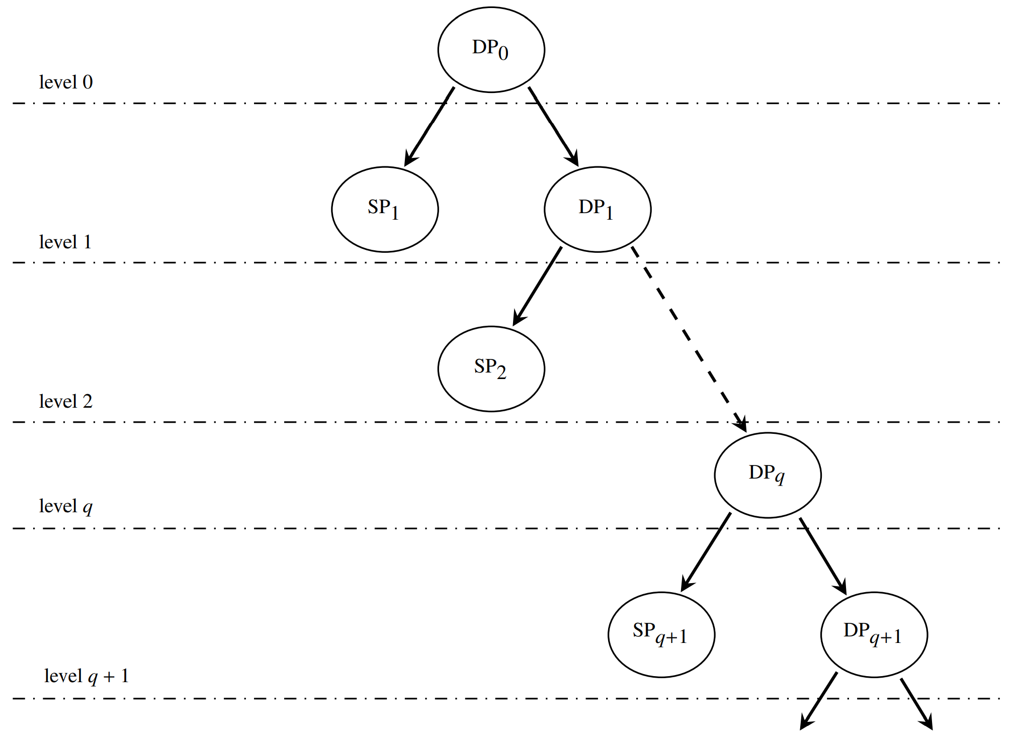
Figure 1: C&S search tree

The C&S procedure is essentially a branch-and-bound algorithm in which a search tree (see Fig. 1) will be constructed during the search. More specifically, the C&S denotes the original problem (1) as $\text{DP}_{0}$ and the best objective value of all feasible solutions found so far as $\text{UB}_{\min}$ (the corresponding feasible solution is denoted as $(x_{\min},y_{\min},z_{\min})$). At the $q$-th ($q\in\mathbb{Z}_{+}$) level of the C&S search tree (see Fig. 1), we first solve the LP relaxation of $\text{DP}_{q}$, denoted its solution by $(x^{*},y^{*},z^{*})$ and the corresponding objective value by $\text{LB}_{q}$.

• If $(x^{*},y^{*},z^{*})$ is an integer vector, then $(x^{*},y^{*},z^{*})$ is an optimal solution of problem $\text{DP}_{q}$ and hence the searching procedure can be terminated;

• If $\text{LB}_{q}\geq\text{UB}_{\min}$, then $(x_{\min},y_{\min},z_{\min})$ must be an optimal solution of problem (1) and hence the searching procedure can also be terminated.

If neither (i) nor (ii) is satisfied, we then decompose the $\text{DP}_{q}$ into two subproblems $\text{SP}_{q+1}$ and $\text{DP}_{q+1}$, which are defined as $\text{DP}_{q}$ with the so-called piercing cuts [31]

$$\sum\limits_{k\in\mathcal{S}}y_{k}\leq\varphi,$$ (11)

and

$$\sum\limits_{k\in\mathcal{S}}y_{k}\geq\varphi+1,$$ (12)

respectively. Here $\varphi$ is a positive integer and $\mathcal{S}$ is a subset of $\mathcal{K}$. A common selection used in [31, 32, 33, 34] is to set $\varphi=0$, making the right subproblem $\text{DP}_{q+1}$ and the left subproblem $\text{SP}_{q+1}$ being a dense problem and a sparse problem (in terms of small solution space). Indeed, for $\text{SP}_{q+1}$, such a selection forces (i) $y_{k}=0$ for all $k\in\mathcal{S}$ and (ii) $x_{i,k}=0$ and $z_{i,k}=0$ for all $i\in\mathcal{I}$ and $k\in\mathcal{S}$ (implied by constraints (1b) and (1d’)). Due to the small solution space, sparse problem $\text{SP}_{q+1}$ can be solved by standard MILP solvers within a reasonable time limit, especially when $|\mathcal{S}|$ is large. Moreover, as far as the sparse problem $\text{SP}_{q+1}$ has a feasible solution, it can provide an upper bound $\text{UB}_{q+1}$ for problem (1). If $\text{UB}_{q+1}<\text{UB}_{\min}$, $\text{UB}_{\min}\coloneqq\text{UB}_{q+1}$ will be updated. The above procedure is repeated until case i) or ii) is satisfied. The details are summarized in Algorithm 1.

We now discuss the selection of $\mathcal{S}$ in (11) and (12), which defines subproblems $\text{SP}_{q+1}$ and $\text{DP}_{q+1}$. A straightforward strategy is to choose the set $\mathcal{S}$ as

$$\mathcal{S}_{1}:=\left\{k\in\mathcal{K}\,:\,y^{*}_{k}=0\right\},$$ (13)

where $y^{*}$, as stated, is the optimal solution of $\text{DP}_{q}$’s relaxation. The rationale behind strategy lies in the fact that an optimal solution to $\text{DP}_{q}$ usually has a number of components that are identical to those of an optimal solution to $\text{DP}_{q}$’s relaxation. Consequently, it is more likely to find a good feasible solution (in terms of small objective value) by solving the sparse problem $\text{SP}_{q+1}$. However, our preliminary experiments showed that due to the (general) degeneracy of the LP relaxation of $\text{DP}_{q}$, such a simple strategy cannot improve the lower bound (returned by solving the LP relaxation of $\text{DP}_{q+1}$) fast enough, leading to a large search tree. For this reason, we use a more sophisticated strategy, suggested by Climer and Zhang [31], to determine $\mathcal{S}$, which is detailed as follows. From the basic LP theory, the reduced cost $r^{*}_{k}$ of a variable $y_{k}$ is a lower bound on the increase of the objective value if the value of this variable is changed by one unit. These reduced costs can be obtained by solving the LP relaxation of $\text{DP}_{q+1}$. Moreover,

• If $y_{k}^{*}=0$, then $r_{k}^{*}\geq 0$;

• If $y_{k}^{*}=1$, then $r_{k}^{*}\leq 0$;

• If $0<y_{k}^{*}<1$, then $r_{k}^{*}=0$.

For more details, we refer to [Dantzig2003, Chapter 5]. Using the reduced costs, we set $\mathcal{S}$ as

$$\mathcal{S}_{2}:=\left\{k\in\mathcal{K}\,:\,r^{*}_{k}\geq\epsilon\right\},$$ (14)

where $\epsilon>0$ that controls the problem size of $\text{SP}_{q+1}$ and the size of C&S’s search tree. Indeed, it follows that $\mathcal{S}_{2}\subseteq\mathcal{S}_{1}$, leading to a relatively large sparse problem $\text{SP}_{q+1}$, as compared to that defined by $\mathcal{S}_{1}$. The larger the $\epsilon$ is, the larger the solution space of $\text{SP}_{q+1}$ is. However, this also enables to obtain a much large better lower bound returned by solving $\text{DP}_{q+1}$’s relaxation (indeed, the difference of the objective values $\text{DP}_{q}$’s and $\text{DP}_{q+1}$’s relaxations is at least $\min\left\{r_{k}\,:\,k\in\mathcal{S}_{2}\right\}\geq\epsilon>0$), yielding a smaller C&S search tree. In our implementation, we set $\epsilon=10^{-4}$.

1 Initialize $\text{UB}_{\min}\coloneqq+\infty$ and $q\coloneqq 0$;

2 while true do

3       Solve the LP relaxation of problem $\text{DP}_{q}$ with the solution $(x^{*},y^{*},z^{*})$ and the objective value $\text{LB}_{q}$;

4       if $\text{\rm LB}_{q}\geq\text{\rm UB}_{\min}$ then

5             Stop and return the optimal solution $(x_{\min},y_{\min},z_{\min})$;

6      if $(x^{*},y^{*},z^{*})$ is an integer vector then

7             Stop and return the optimal solution $({x}^{*},{y}^{*},{z}^{*})$;

8      Use the piercing cuts (11) and (12) to decompose $\text{DP}_{q}$ into two subproblems $\text{SP}_{q+1}$ and $\text{DP}_{q+1}$;

9       Solve $\text{SP}_{q+1}$ to optimality by an MILP solver and denote its solution and objective value by $(x^{\prime},y^{\prime},z^{\prime})$ and $\text{UB}_{q+1}$;

10       if $\text{\rm UB}_{q+1}<\text{\rm UB}_{\min}$ then

11             Update $(x_{\min},y_{\min},z_{\min})\coloneqq(x^{\prime},y^{\prime},z^{\prime})$ and $\text{UB}_{\min}\coloneqq\text{UB}_{q+1}$;

12            

13      Set $q\coloneqq q+1$;

Algorithm 1 C&S algorithm

3.2 An improved relaxation problem and the cutting plane approach

The LP relaxation of problem (1), obtained by ignoring the integrality requirement on all decision variables, is as follows:

$$\mathop{\mathrm{min}}\ \sum_{i\in\mathcal{I}}\sum_{k\in\mathcal{K}}c^{\rm alloc}_{i,k}n_{i,k}+\sum_{k\in\mathcal{K}}c^{\rm run}_{k}y_{k}+\sum\limits_{i\in\mathcal{I}}\sum\limits_{k\in\mathcal{K}}c^{\rm mig}_{i,k}z_{i,k}$$ (15a)

s.t. $$\eqref{eq:resource},\eqref{eq:allocation_general},\eqref{eq:migration1},$$ (15b)

$$x_{i,k},~{}z_{i,k}\in\mathbb{R_{+}},~{}x_{i,k}\leq v_{i,k},~{}\forall~{}i\in\mathcal{I},~{}\forall~{}k\in\mathcal{K},$$ (15c)

$$y_{k}\in[0,1],~{}\forall~{}k\in\mathcal{K}.$$ (15d)

However, the feasible region of LP relaxation (15) is actually enlarged compared with that of the original problem (1). As a result, this relaxation usually provides a weak lower bound, leading to a large C&S search tree; see Section 4.3 further ahead. To overcome this weakness, we present a new relaxation that has a much more compact feasible region and hence can provide a much stronger lower bound, as compared with relaxation (15). Then we provide a cutting plane approach to solve this newly proposed relaxation.

3.2.1 An improved relaxation problem

To proceed, we observe that in problem (1), it is required that

$$(x_{\cdot,k},y_{k}) \in\mathcal{X}(r,k):=\bigg{\{}(x_{\cdot,k},y_{k})\in\mathbb{Z}_{+}^{|\mathcal{I}|}\times\{0,1\}:$$

$$\sum\limits_{i\in\mathcal{I}}u_{i,r}x_{i,k}\leq s_{k,r}y_{k},~{}x_{i,k}\leq v_{i,k},~{}\forall~{}i\in\mathcal{I}~{}\bigg{\}},$$ (16)

for all $k\in\mathcal{K}$ and $r\in\mathcal{R}$. However, in problem (15), such a requirement is relaxed to

$$(x_{\cdot,k},y_{k})\in\mathcal{X}_{\text{L}}(r,k):=\bigg{\{}(x_{\cdot,k},y_{k})\in\mathbb{R}_{+}^{|\mathcal{I}|}\times[0,1]:$$ (17)

$$\qquad\qquad\sum\limits_{i\in\mathcal{I}}u_{i,r}x_{i,k}\leq s_{k,r}y_{k},~{}x_{i,k}\leq v_{i,k},~{}\forall~{}i\in\mathcal{I}~{}\bigg{\}},$$

making a much larger feasible region for $(x_{\cdot,k},y_{k})$. Notice that by (16) and $\mathcal{X}(r,k)\subseteq\operatorname{conv}(\mathcal{X}(r,k))$,

$$(x_{\cdot,k},y_{k})\in\operatorname{conv}(\mathcal{X}(r,k)),$$ (18)

must hold for every feasible solution of problem (1). Therefore, our first refinement of relaxation (15) is to replace (17) with (18). As $\operatorname{conv}(\mathcal{X}(r,k))\subseteq\mathcal{X}_{\text{L}}(r,k)$, such a refinement can possibly make a smaller feasible region for $(x_{\cdot,k},y_{k})$ when relaxing the integrality requirement on variables $(x_{\cdot,k},y_{k})$.

Next, we pose more restrictions on vector $y$. In particular, for $r\in\mathcal{R}$, adding all the constraints in (1b) for all $k\in\mathcal{K}$ and using constraint (1c), we obtain

$$\sum\limits_{k\in\mathcal{K}}s_{k,r}y_{k}\geq\sum_{i\in\mathcal{I}}d_{i}u_{i,r}.$$ (19)

The above constraint requires that the total resources of activated servers should be larger than or equal to the total required resources of all VMs. We remark that in problem (1), it is required that

$$y\in\mathcal{Y}(r):=\biggl{\{}y\in\{0,1\}^{|\mathcal{K}|}\,:\,\eqref{totalcap}\biggr{\}},~{}\forall~{}r\in\mathcal{R},$$ (20)

while in relaxation (15), $y\in\{0,1\}^{|\mathcal{K}|}$ is relaxed to $y\in[0,1]^{|\mathcal{K}|}$, and as a result, it follows

$$y\in\mathcal{Y}_{\text{L}}(r):=\biggl{\{}y\in[0,1]^{|\mathcal{K}|}\,:\,\eqref{totalcap}\biggr{\}},~{}\forall~{}r\in\mathcal{R}.$$ (21)

Our second refinement of relaxation (15) is to enforce

$$y\in\operatorname{conv}(\mathcal{Y}(r)),~{}\forall~{}r\in\mathcal{R}.$$ (22)

Similarly, as $\operatorname{conv}(\mathcal{Y}(r))\subseteq\mathcal{Y}_{\text{L}}(r)$, enforcing (22) in relaxation (15) can possibly make a smaller feasible region for vector $y$ when relaxing the integrality requirement on variables $y$.

With the above two refinements, we obtain the new relaxation for problem (1):

$$\mathop{\mathrm{min}}\ \sum_{i\in\mathcal{I}}\sum_{k\in\mathcal{K}}c^{\rm alloc}_{i,k}n_{i,k}+\sum_{k\in\mathcal{K}}c^{\rm run}_{k}y_{k}+\sum\limits_{i\in\mathcal{I}}\sum\limits_{k\in\mathcal{K}}c^{\rm mig}_{i,k}z_{i,k}$$ (23a)

s.t. $$\eqref{eq:allocation_general},\eqref{eq:migration1},\eqref{eq:varX_lp},\eqref{eq:varY_lp},$$ (23b)

$$(x_{\cdot,k},y_{k})\in\operatorname{conv}(\mathcal{X}(r,k)),~{}\forall~{}k\in\mathcal{K},~{}\forall~{}r\in\mathcal{R},$$ (23c)

$$y\in\operatorname{conv}(\mathcal{Y}(r)),~{}\forall~{}r\in\mathcal{R}.$$ (23d)

As discussed, (23c) and (23d) make a smaller feasible region for the decision variables in relaxation (23), as compared with that of relaxation (15). As a result, relaxation (23) can provide a tighter lower bound and hence makes a smaller C&S search tree; see Section 4.3 further ahead.

3.2.2 The cutting plane approach to solve (23)

$\operatorname{conv}(\mathcal{X}(r,k))$ and $\operatorname{conv}(\mathcal{Y}(r))$ are polytopes that can be expressed by a finite number of inequalities, called facet-defining inequalities; see, e.g, [36, Proposition 8.1]. However, it is not practical to solve problem (23) by enumerating all inequalities of $\operatorname{conv}(\mathcal{X}(r,k))$ and $\operatorname{conv}(\mathcal{Y}(r))$ due to the following two reasons. First, it is computationally expensive to find all inequalities that are required to describe $\operatorname{conv}(\mathcal{X}(r,k))$ and $\operatorname{conv}(\mathcal{Y}(r))$. Second, the numbers of inequalities that describe $\operatorname{conv}(\mathcal{X}(r,k))$ and $\operatorname{conv}(\mathcal{Y}(r))$ are potentially huge (usually exponential), making it hard to solve problem (23). Due to this, we use a cutting plane approach to solve problem (23), which is used, e.g., in [37] in the context of solving the generalized assignment problem. This approach is detailed as follows. First, we solve relaxation (15) to obtain its solution $(x^{*},y^{*})$. Then, we solve the separation problem, that is, either (i) find a set of inequalities which are valid for $\operatorname{conv}(\mathcal{X}(r,k))$, $k\in\mathcal{K}$ and $r\in\mathcal{R}$, and $\operatorname{conv}(\mathcal{Y}(r))$, $r\in\mathcal{R}$, but can cut off point $(x^{*},y^{*})$ (called violated inequalities) or (ii) prove $(x^{*},y^{*})\in\operatorname{conv}(\mathcal{X}(r,k))$ for all $k\in\mathcal{K}$ and $r\in\mathcal{R}$ , and $y^{*}\in\operatorname{conv}(\mathcal{Y}(r))$ for all $r\in\mathcal{R}$. For case (i), we add the violated inequalities into relaxation (15) and solve it again. For case (ii), $(x^{*},y^{*})$ must be an optimal solution of problem (23). The above procedure is iteratively applied until case (ii) holds. In the following, we demonstrate how to solve the separation problem in detail.
$\bullet$ Integer knapsack set
To solve the separation problem over $\operatorname{conv}(\mathcal{X}(r,k))$ or $\operatorname{conv}(\mathcal{Y}(r))$, it suffices to consider the separation problem over $\operatorname{conv}(\mathcal{X})$, where $\mathcal{X}$ is the generic integer knapsack set:

$$\mathcal{X}=\left\{x\in\mathbb{Z}_{+}^{|\mathcal{N}|}:\sum_{i\in\mathcal{N}}a_{i}x_{i}\leq b,~{}x_{i}\leq v_{i},~{}\forall~{}i\in\mathcal{N}\right\},$$

$a_{i}\geq 0$, $a_{i}v_{i}\leq b$ for all $i\in\mathcal{N}$, and $b\geq 0$. Indeed, by replacing variable $y_{k}$ with $y^{\prime}_{k}=1-y_{k}$ for all $k\in\mathcal{K}$ in $\mathcal{Y}(r)$, we obtain the so-called binary knapsack set

$$\mathcal{Y}^{\prime}(r)=\left\{y^{\prime}\in\left\{0,1\right\}^{\left|\mathcal{K}\right|}:\sum_{k\in\mathcal{K}}s_{k,r}y^{\prime}_{k}\leq\sum_{k\in\mathcal{K}}s_{k}-\sum_{i\in\mathcal{I}}d_{i}u_{i,r}\right\},~{}\forall~{}r\in\mathcal{R},$$

which is a special case of integer knapsack set, that is, $v_{i}=1$, $i\in\mathcal{N}$ in $\mathcal{X}$. We remark that inequality $\sum_{k\in\mathcal{K}}\alpha_{k,r}y^{\prime}_{k}\leq\beta_{r}$ is valid for $\operatorname{conv}(\mathcal{Y}^{\prime}(r))$ if and only if $\sum_{k\in\mathcal{K}}\alpha_{k,r}(1-y_{k})\leq\beta_{r}$ is valid for $\operatorname{conv}(\mathcal{Y}(r))$. The set $\mathcal{X}(r,k)$ is a form of

$$\mathcal{X}_{y}=\left\{(x,y)\in\mathbb{Z}_{+}^{\left|\mathcal{N}\right|}\times\left\{0,1\right\}:\sum_{i\in\mathcal{N}}a_{i}x_{i}\leq by,~{}x_{i}\leq v_{i},~{}\forall~{}i\in\mathcal{N}\right\}.$$

The following proposition shows that all nontrivial facet-defining inequalities of $\operatorname{conv}(\mathcal{X}_{y})$ can be derived from facet-defining inequalities of $\operatorname{conv}(\mathcal{X})$.

Proposition 1.

(i) All facet-defining inequalities of $\operatorname{conv}(\mathcal{X})$, except $x_{i}\geq 0$, $i\in\mathcal{N}$, are of the form $\sum_{i\in\mathcal{N}}\pi_{i}x_{i}\leq\pi_{0}$ with $\pi_{i}\geq 0$, $i\in\mathcal{N}$, and $\pi_{0}>0$; and (ii) all facet-defining inequalities of $\operatorname{conv}(\mathcal{X}_{y})$, except $x_{i}\geq 0$, $i\in\mathcal{N}$, $y\leq 1$, have the form $\sum_{i\in\mathcal{N}}\pi_{i}x_{i}\leq\pi_{0}y$, where $\sum_{i\in\mathcal{N}}\pi_{i}x_{i}\leq\pi_{0}$ is a facet-defining inequality of $\operatorname{conv}(\mathcal{{X}})$ differing from inequalities $x_{i}\geq 0$, $i\in\mathcal{N}$.

Proof.

The proof is relegated to the appendix. ∎

Let $(x^{*},y^{*})\in\mathbb{R}_{+}^{|\mathcal{N}|}\times[0,1]$. If $y^{*}=0$, then $x^{*}=\bm{0}$ and thus $(x^{*},y^{*})\in\operatorname{conv}(\mathcal{X}_{y})$. Otherwise, by Proposition 1, it follows that $(x^{*},y^{*})\in\operatorname{conv}(\mathcal{X}_{y})$ if and only if $\bar{x}\in\operatorname{conv}(\mathcal{X})$ where $\bar{x}_{i}=\frac{x^{*}_{i}}{y^{*}}$ for all $i\in\mathcal{N}$. Based on the above discussion, we shall concentrate on the separation problem over $\operatorname{conv}(\mathcal{X})$ in the following.
$\bullet$ Exact separation for integer knapsack polytope $\operatorname{conv}(\mathcal{X})$
Next, we solve the separation problem of polytope $\operatorname{conv}(\mathcal{X})$, that is, either construct a hyperplane separating point $\bar{x}$ from the $\operatorname{conv}(\mathcal{X})$ strictly, i.e.,

$$\pi^{\top}x\leq\pi_{0},~{}\forall~{}x\in\operatorname{conv}(\mathcal{X})~{}(\text{or equivalently},~{}\forall~{}x\in\mathcal{X}),$$ (24)

and

$${\bar{x}}^{\top}\pi>\pi_{0},$$ (25)

or prove that none exists, i.e., $\bar{x}\in\operatorname{conv}(\mathcal{X})$. This separation problem can be reduced to the following LP problem

$$\omega(\bar{x})=\max_{(\pi,\pi_{0})\in\mathbb{R}^{|\mathcal{N}|+1}}\left\{{\bar{x}}^{\top}\pi-\pi_{0}:\pi^{\top}x\leq\pi_{0},~{}\forall~{}x\in\mathcal{X}\right\},$$ (26)

If $\omega(\bar{x})\leq 0$, we must have $\bar{x}\in\operatorname{conv}(\mathcal{X})$; otherwise, $\pi^{\top}x\leq\pi_{0}$ is a valid inequality violated by $\bar{x}$. By Proposition 1 (i), we can, without loss of generality, add $\pi_{i}\geq 0$ for all $i\in\mathcal{N}$ and $\pi_{0}>0$ into problem (26). Moreover, we can further normalize $\pi_{0}$ as $1$ (as $\pi_{0}>0$) and obtain the following equivalent problem

$$\omega(\bar{x})=\max_{\pi\in\mathbb{R}^{|\mathcal{N}|}_{+}}\left\{{\bar{x}}^{\top}\pi:\pi^{\top}x\leq 1,~{}\forall~{}x\in\mathcal{X}\right\}.$$ (27)

In particular, letting $\pi^{*}$ be an optimal solution of (27), if ${\bar{x}}^{\top}\pi^{*}\leq 1$, we prove $\bar{x}\in\operatorname{conv}(\mathcal{X})$; otherwise, we find the inequality ${\pi^{*}}^{\top}x\leq 1$ violated by $\bar{x}$. One weakness of problem (27) is its large problem size. Indeed, the number of constraint $\pi^{\top}x\leq 1$ may be exponential as the points in $\mathcal{X}$ may be exponential. Consequently, from a computational perspective, it is not practical to solve the separation problem when all constraints are explicitly expressed. For this reason, we use the row generation method, an iterative approach that starts with a subset of constraints and then dynamically adds other constraints when violations occur [38]. More specifically, we first choose an initial subset

$$\mathcal{U}=\left\{v_{i}\bm{e}^{i}\,:\,i\in\mathcal{N}\right\}\subseteq\mathcal{X},$$ (28)

where $\bm{e}^{i}$ is the $i$-th $\left|\mathcal{N}\right|$-dimensional unit vector, and solve the partial separation problem defined by this subset $\mathcal{U}$:

$$\omega^{\prime}(\bar{x})=\max_{{\pi\in\mathbb{R}^{|\mathcal{N}|}_{+}}}\left\{{\bar{x}}^{\top}\pi:\pi^{\top}x\leq 1,~{}\forall~{}{x}\in\mathcal{U}\right\}.$$ (29)

Let $\pi^{*}$ be an optimal solution of (29). If $\omega^{\prime}\left(\bar{x}\right)\leq 1$, we prove $\bar{x}\in\operatorname{conv}(\mathcal{X})$ (as $\mathcal{U}\subseteq\mathcal{X}$); otherwise, we check whether ${\pi^{*}}^{\top}x\leq 1$ holds for all $x\in\mathcal{X}$ by solving the following bounded knapsack problem

$${h}^{*}\in\operatorname*{arg\,max}_{{h}}\left\{{\pi^{*}}^{\top}h:\forall~{}{h}\in\mathcal{X}\right\}.$$ (30)

(i) If ${\pi^{*}}^{\top}{h^{*}}\leq 1$, ${\pi^{*}}^{\top}x\leq 1$ holds for all $x\in\mathcal{X}$; (ii) otherwise, we add $h^{*}$ into $\mathcal{U}$ and solve problem (29) again. The above procedure is iteratively applied until case (i) holds. The row generation method is summarized in Algorithm 2.

Input: The set $\mathcal{X}$ and a solution ${\bar{x}}$.

Output: Find a violated inequality ${\pi^{*}}^{\top}x\leq 1$ separating ${\bar{x}}$ from $\operatorname{conv}(\mathcal{X})$ or conclude that ${\bar{x}}\in\operatorname{conv}(\mathcal{X})$.

1 Choose an initial subset $\mathcal{U}$ as in (28);

2 Solve the partial separation problem (29) to obtain its solution $\pi^{*}$;

3 If ${\bar{x}}^{\top}\pi^{*}\leq 1$, conclude ${\bar{x}}\in\operatorname{conv}(\mathcal{X})$ and stop; otherwise, solve the bounded knapsack problem (30) to obtain the solution $h^{*}$;

If ${\pi^{*}}^{\top}{h^{*}}>1$, set $\mathcal{U}\coloneqq\mathcal{U}\cup\{{h}^{*}\}$ and go to step 2; otherwise, stop and return the violated inequality ${\pi^{*}}^{\top}x\leq 1$;

Algorithm 2 The row generation method to solve the separation problem of $\operatorname{conv}(\mathcal{X})$.

We remark that problem (30) is an integer knapsack problem which is generally NP-hard. However, it can be solved by the dynamic programming algorithm in [39], which runs in pseudo-polynomial time but is quite efficient in practice. In addition, problem (30) may have multiple optimal solutions. We follow [40] to choose a solution with large values $h^{*}$. This strategy provides a much stronger inequality ${\pi}^{\top}h^{*}\leq 1$ for problem (29), which effectively decreases the number of iterations in Algorithm 2. For more details, we refer to [40].
$\bullet$ Efficient implementation
In each iteration of Algorithm 2, we need to solve the LP problem (29), which is still time-consuming, especially when the dimension of $\mathcal{X}$ is large. Below, we introduce two simple techniques to reduce the dimension of $\mathcal{X}$.

First, we can aggregate multiple variables with the same coefficient into a single variable. Specifically, suppose that $a_{i}$, $i\in\mathcal{N}^{\prime}$, are equal. Then replacing $\sum_{i\in\mathcal{N}^{\prime}}x_{i}$ by a new variable $\delta$ (with $\delta\leq\sum_{i\in\mathcal{N}^{\prime}}v_{i}$) in $\mathcal{X}$, we obtain a new set $\mathcal{X}^{\prime}$. After constructing a valid inequality for $\mathcal{X}^{\prime}$, we substitute $\delta=\sum_{i\in\mathcal{N}^{\prime}}x_{i}$ into this inequality and obtain a valid inequality for $\mathcal{X}$. In our experience, this simple technique effectively reduces the CPU time spent by Algorithm 2, especially when most coefficients in $\mathcal{X}$ are equal. The second technique to reduce the dimension of $\mathcal{X}$ comes from Vasilyev et al. [38], which consists of two steps. In the first step, the separation problem over a projected polytope $\operatorname{conv}(\mathcal{X}({\bar{x}}))$ is solved to obtain a valid inequality (violated by $\bar{x}$):

$$\sum_{i\in\mathcal{N}_{\rm R}}\pi_{i}x_{i}\leq 1,$$ (31)

where

$$\mathcal{X}({\bar{x}})=\left\{{x}\in\mathbb{Z}_{+}^{\left|\mathcal{N}_{\rm R}\right|}:\sum_{i\in\mathcal{N}_{\rm R}}a_{i}x_{i}\leq\bar{b},~{}x_{i}\leq v_{i},~{}\forall~{}i\in\mathcal{N}_{\rm R}\right\},$$ (32)

$\mathcal{N}_{\rm L}=\left\{i\in\mathcal{N}:\bar{x}_{i}=0\right\}$, $\mathcal{N}_{\rm U}=\left\{i\in\mathcal{N}:\bar{x}_{i}=v_{i}\right\}$, $\mathcal{N}_{\rm R}=\mathcal{N}\backslash(\mathcal{N}_{\rm L}\cup\mathcal{N}_{\rm U})$, and $\bar{b}=b-\sum_{i\in\mathcal{N}_{\rm U}}a_{i}v_{i}$. It can be expected that the separation problem over $\operatorname{conv}(\mathcal{X}({\bar{x}}))$ is easier to solve than that over $\operatorname{conv}(\mathcal{X})$, especially when the number of fixed variables $|\mathcal{N}_{\text{L}}|+|\mathcal{N}_{\text{U}}|$ is large. In the second step, we derive a valid inequality

$$\sum_{i\in\mathcal{N}_{\rm R}}\pi_{i}x_{i}+\sum_{i\in\mathcal{N}_{\rm L}}{\pi}_{i}x_{i}+\sum_{i\in\mathcal{N}_{\rm U}}{\pi}_{i}x_{i}\leq 1+\sum_{i\in\mathcal{N}_{\rm U}}{\pi}_{i}v_{i},$$ (33)

for $\operatorname{conv}(\mathcal{X})$ using sequential lifting; see, e.g., [41, 38, 42, 43, 44] for a detailed discussion of sequential lifting.

4 Numerical results

In this section, we present simulation results to illustrate the effectiveness and efficiency of the proposed formulation (1) and the proposed C&S algorithm for solving VMCPs. More specifically, we first perform numerical experiments to compare the performance of solving the proposed formulation (1) and the two existing formulations in [5] and [15] by standard MILP solvers. Then, we present some simulation results to demonstrate the efficiency of the proposed C&S algorithm for solving VMCPs over standard MILP solvers. Finally, we evaluate the performance of our proposed C&S algorithm under different problem parameters.

In our implementation, the proposed C&S was implemented in C++ linked with IBM ILOG CPLEX optimizer 20.1.0 [27]. The time limit and relative gap tolerance were set to 7200 seconds and 0%, respectively, in all experiments. The cutting plane approach was stopped if the optimal value of the LP relaxation problem of VMCP is improved by less than 0.05% between two adjacent calls. Unless otherwise specified, all other CPLEX parameters were set to their default values. All experiments were performed on a cluster of Intel(R) Xeon(R) Gold 6140 @ 2.30GHz computers, with 192 GB RAM, running Linux (in 64 bit mode).

4.1 Testsets

We tested all algorithms on problem instances with 5 VM types and 10 server types with different features (CPU, RAM, and Bandwidth resources and power consumption), as studied in [15]. The VM types and server types are in line with industry standards and are described in Tables 2 and 3, respectively.

The basic VMCP (1) instances are constructed using the same procedure in [15]. Specifically, each instance has an equal number of servers of each type. The number of servers $|\mathcal{K}|$ is selected from $\{250,500,750,1000\}$. For each server $k$, we iteratively assign a uniform random number $n_{i,k}$ (satisfying $n_{i,k}\in\{0,\ldots,\lfloor\frac{s_{k,r}}{u_{i,r}}\rfloor\}$) of VMs of type $i$ until the maximum usage of the available resource (CPU, RAM, and Bandwidth) load $\sigma_{k}$, defined by,

$$\sigma_{k}=\max\biggl{\{}\frac{\sum_{i\in\mathcal{I}}u_{i,r}n_{i,k}}{s_{k,r}}:\forall~{}r\in\mathcal{R}\biggr{\}},$$ (34)

exceeds a predefined value $\alpha$. In general, the larger the $\alpha$, the more VMs will be constructed. We choose $\alpha\in\{20\%,40\%\}$. In our test, we attempt to minimize the total power consumption of the servers. As shown in [15, 45, 8], the power consumption of a server can be represented by the following linear model:

$$P_{k}=P_{{\rm idle},k}+\left(P_{{\rm max},k}-P_{{\rm idle},k}\right)U_{k},$$ (35)

where $P_{{\rm idle},k}$ is the idle power consumption (at the idle state) of server $k$, $P_{{\rm max},k}$ is the maximum power consumption (at the peak state) of server $k$, and $U_{k}$ ($U_{k}\in\left[0,1\right]$) is the CPU utilization of server $k$. As such, (i) the activation cost $c^{\rm run}_{k}$ is set to the idle power consumption of server $k$, which is equal to 60% of the maximum power consumption, as assumed by [15]; and (ii) the allocation cost $c^{\rm alloc}_{i,k}$ is set to $\left(P_{{\rm max},k}-P_{{\rm idle},k}\right)\frac{u_{i,{\rm CPU}}}{s_{k,{\rm CPU}}}$. As illustrated in Section 2, $c^{\rm mig}_{i,k}$ is set to $c^{\rm alloc}_{i,k}$ in the experiments.

The extended VMCP (i.e., problem (1) with constraints (2)-(8)) instances are constructed based on the basic VMCP instances described above with the parameters for constraints (2)-(8) described as follows. For constraints (2) and (3), parameter $d^{\rm new}_{i}$ is obtained by setting existing VMs as new incoming VMs with a probability $\beta$, chosen in {35%, 45%}. For constraint (4), parameter ℓ is set as $\eta\sum\limits_{i\in\mathcal{I}}\sum\limits_{k\in\mathcal{K}}n_{i,k}$ where $\eta$ is chosen in $\left\{30\%,40\%\right\}$. For constraints (5) or (6), the maximum number of VMs on each server $k$, $m_{k}$, is set to $\lambda\max\limits_{i\in\mathcal{I}}\min\limits_{r\in\mathcal{R}}\lfloor\frac{s_{k,r}}{u_{i,r}}\rfloor$, where $\lambda\in\left\{85\%,90\%\right\}$. Notice that $\min\limits_{r\in\mathcal{R}}\lfloor\frac{s_{k,r}}{u_{i,r}}\rfloor$ is the maximum number of VMs of type $i$ that can be allocated to a given server $k$, and hence $\max\limits_{i\in\mathcal{I}}\min\limits_{r\in\mathcal{R}}\lfloor\frac{s_{k,r}}{u_{i,r}}\rfloor$ is the maximum number of VMs of a single type that can be allocated to a given server $k$. For constraints (7) and (8), we randomly choose the element $k\in\mathcal{K}$ to subset $\mathcal{K}(i)$, $i\in\mathcal{I}$, with a probability $\theta$, chosen in $\{5\%,10\%\}$.

For each fixed $|\mathcal{K}|\in\{250,500,750,1000\}$ and $\alpha\in\{20\%,40\%\}$, 50 basic VMCP instances are randomly generated, leading to an overall 400 basic VMCP instances testbed. In addition, for each fixed $|\mathcal{K}|\in\{250,500,750,1000\}$, $\alpha\in\{20\%,40\%\}$, $\beta\in\{35\%,45\%\}$, $\eta\in\{30\%,40\%\}$, $\lambda\in\{85\%,90\%\}$, and $\theta\in\{5\%,10\%\}$, 10 extended VMCP instances are randomly generated, leading to an overall $1280$ extended VMCP instances testbed.

Table 2: The five VM types.

Type	CPU	RAM (GB)	Bandwidth (Mbps)
VM 1	1	1	10
VM 2	2	4	100
VM 3	4	8	300
VM 4	6	12	1000
VM 5	8	16	1200

Table 3: The ten server types.

Type	CPU	RAM (GB)	Bandwidth (Mbps)	Maximum power consumption (W)
Server 1	4	8	1000	180
Server 2	8	16	1000	200
Server 3	10	16	2000	250
Server 4	12	32	2000	250
Server 5	14	32	2000	280
Server 6	14	32	2000	300
Server 7	16	32	4000	300
Server 8	16	64	4000	350
Server 9	18	64	4000	380
Server 10	18	64	4000	410

4.2 Efficiency of the proposed formulation

In this subsection, we present computational results to illustrate the efficiency of the proposed formulation (1) over those in [5] and [15] (i.e., formulations (9) and (10)). Table 4 summarized the computational results of the three formulations solved by CPLEX. We report the number of instances that can be solved to optimality witnin the given time limit (#S), the average CPU time (T), and the average number of constraints and variables (#CONS and #VARS, respectively).

[b] $\left(\left|\mathcal{K}\right|,\alpha\right)$ #VM Proposed formulation (1) Formulation in Speitkamp and Bichler [5] Formulation in Mazumdar and Pranzo [15] #S T #CONS #VARS #S T #CONS #VARS #S T #CONS #VARS (250, 20%) 959 50 1.5 2005 2750 46 905.8 241459 479750 45 574.3 2000 312750 (250, 40%) 1163 49 2.9 2005 2750 37 1664.7 292663 581750 37 870.7 2000 312750 (500, 20%) 1924 50 3.9 4005 5500 20 5179.7 965424 1924500 20 3782.5 4000 1250500 (500, 40%) 2310 45 12.5 4005 5500 8 5266.9 1158810 2310500 13 4302.6 4000 1250500 (750, 20%) 2855 41 38.4 6005 8250 1 6996.1 2146355 4283250 1 6962.0 6000 2813250 (750, 40%) 3493 31 108.7 6005 8250 1 6998.3 2625493 5240250 3 6825.0 6000 2813250 (1000, 20%) 3832 36 67.7 8005 11000 0 - 3838832 7665000 0 - 8000 5001000 (1000, 40%) 4655 23 316.2 8005 11000 2 7038.0 4662655 9311000 1 7198.1 8000 5001000 All 325 19.5 115 4227.8 120 3449.4

Table 4: Comparison results of the proposed formulation (1) with existing formulations in [5] and [15]

• In the table, “-” means that the average CPU time reaches the time limit.

As expected, (i) the numbers of variables and constraints in the proposed formulation (1) are much smaller than those in [5]; and (ii) the number of variables in the proposed formulation (1) is also much smaller than the one in [15], but the numbers of constraints in the two formulations are fairly equal. Consequently, it can be clearly seen that it is much more efficient to solve formulation (1) than those in [5] and [15]. More specifically, using the proposed formulation (1), 325 instances (among 400 instances) can be solved to optimality. In sharp contrast, using the formulations in [5] and [15], only 115 and 120 instances can be solved to optimality, respectively. Indeed, for large-scale cases (e.g., $|\mathcal{K}|=750,1000$), only a few instances can be solved to optimality by using the two existing formulations in [5] and [15]. Moreover, as observed in Table 4, compared with the formulations in [5] and [15], the CPU time taken by solving the proposed formulation (1) is much smaller (19.5 seconds versus 4227.8 seconds and 3449.4 seconds). From this computational result, we can conclude that formulation (1) significantly outperforms the formulations in [5] and [15] in terms of solution efficiency.

4.3 Efficiency of the proposed $C\&S$ algorithm

In this subsection, we compare the performance of the proposed C&S algorithm with the approach using the MILP solver CPLEX (called CPX). In addition, to address the advantage of embedding the proposed relaxation (23) into the C&S algorithm, we compare C&S with C&S’ algorithm, in which the LP relaxation (15) is used, to solve VMCPs.

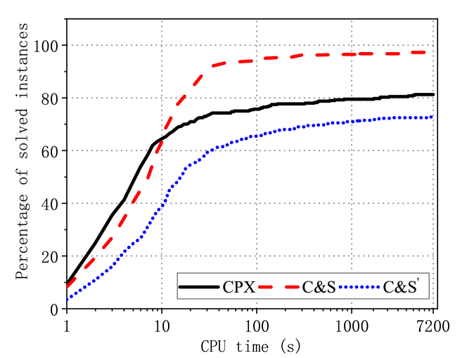
Figure 2: Comparison of the CPU time between CPX, C&S, and C&S’ on basic VMCPs.

Figs. 2-3 plot the performance profiles of the three settings CPX, C&S, and C&S’. Each point with coordinates $(a,b)$ in a line represents that for $b\%$ of the instances, the CPU time is less than or equal to $a$ seconds. From Figs. 2-3, CPX can solve more basic VMCP instances within 10 seconds and more extended VMCP instances within 5 seconds, respectively. This shows that CPX performs a bit better than C&S for easy instances. However, for the hard instances, C&S significantly outperforms CPX, especially for basic VMCPs. In particular, C&S can solve 97% basic VMCP instances to optimality while CPX can solve only 81% basic VMCP instances to optimality.

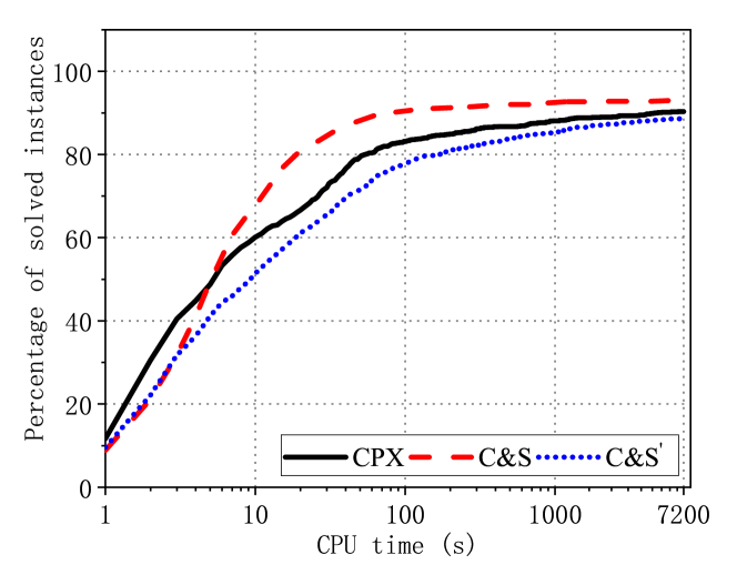
Figure 3: Comparison of the CPU time between CPX, C&S, and C&S’ on extended VMCPs.

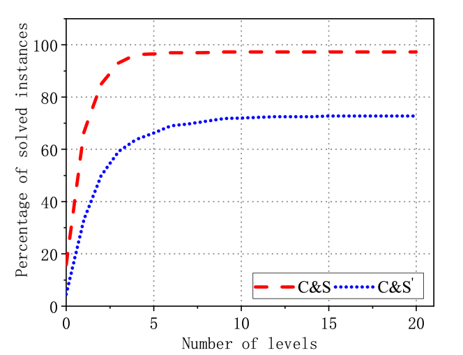
Figure 4: Comparison of the number of levels of the search tree between C&S and C&S’ on basic VMCPs.

In addition, from the two figures, we can conclude that the performance of C&S is much better than C&S’ for basic and extended VMCPs. This indicates that the proposed compact relaxation (23) has a significantly positive performance impact on the C&S approach.

To gain more insight into the computational efficiency of C&S over C&S’, we compare the numbers of levels of the cut-and-solve search trees returned by C&S and C&S’.

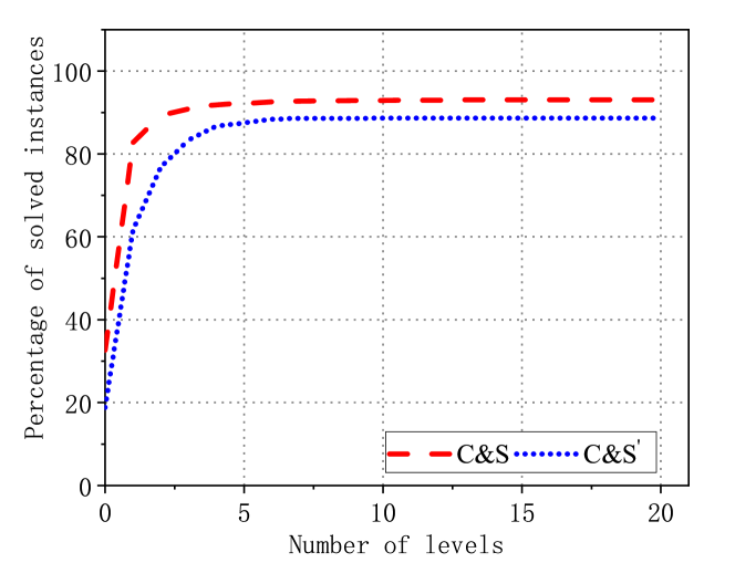
Figure 5: Comparison of the number of levels of the search tree between C&S and C&S’ on extended VMCPs.

The results for the basic and extended VMCP instances are summarized in Figs. 4 and 5, respectively. From the two figures, we can conclude that the number of levels returned by C&S is much less than that returned by C&S’, especially for basic VMCP instances. More specifically, more than 97% of the basic VMCP instances can be solved by C&S within 5 levels while only about 70% of the basic VMCP instances can be solved by C&S’ within 20 levels. This shows the advantage of the proposed relaxation (23), i.e., it can effectively reduces the C&S search tree size.

From the above computational results, we can conclude that (i) the proposed C&S algorithm is much more effective than standard MILP solver, especially for the hard instances; (ii) the proposed relaxation (23) can effectively reduce the size of the C&S search tree, which plays a crucial role in the efficiency of the proposed C&S algorithm.

4.4 Performance comparison of the proposed C&S algorithm

To gain more insights into the performance of the proposed C&S algorithm, we compare the performance of C&S on instances with different numbers of servers $\left|\mathcal{K}\right|$ and different loads $\alpha$ (the higher the load $\alpha$, the larger the number of VMs).

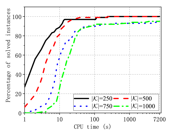
Figure 6: Comparison of the CPU time for C&S on basic VMCPs with different numbers of servers $\left|\mathcal{K}\right|$.

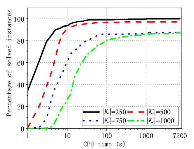
Figure 7: Comparison of the CPU time for C&S on extended VMCPs with different numbers of servers $\left|\mathcal{K}\right|$.

Figs. 6 and 7 plot performance profiles of CPU time, grouped by the number of servers $\left|\mathcal{K}\right|$, for the basic and extended VMCPs, respectively. As expected, the CPU time of C&S generally increases with the number of servers $\left|\mathcal{K}\right|$ for both basic and extended VMCPs. This is reasonable as the problem size and the search space grow with the number of servers. Nevertheless, even for the largest case ($|\mathcal{K}|=1000$), C&S can still solve 95% of basic VMCP instances and 87% of extended VMCP instances to optimality, respectively, which shows the scalability of the proposed C&S with the increasing number of servers.

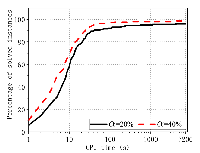
Figure 8: Comparison of the CPU time for C&S on basic VMCPs with different loads $\alpha$.

Next, we compare the results for basic and extended VMCPs with loads $\alpha=20\%$ and $\alpha=40\%$. The results for basic and extended VMCPs are summarized in Figs. 8 and 9, respectively. We observe that the CPU time does not increase with the increasing value of $\alpha$ for basic VMCPs. Even in extended VMCPs, the CPU time of solving instances with load $\alpha=40\%$ is only slightly larger than that of solving instances with load $\alpha=20\%$. However, the same behavior cannot be observed in the computational results returned by CPX (as illustrated in Table 4, the CPU time of using CPX to solve the basic VMCPs with $\alpha=20\%$ is smaller than that of using CPX to solve the basic VMCPs with $\alpha=40\%$). This shows another advantage of the proposed C&S, i.e., a higher load $\alpha$ does not lead to a larger CPU time for solving VMCPs.

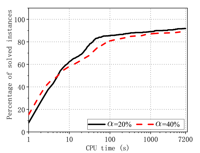
Figure 9: Comparison of the CPU time for C&S on extended VMCPs with different loads $\alpha$.

5 Conclusion and remarks

In this paper, we have proposed new problem formulations for VMCP which minimized the summation of server activation, VM allocation, and migration costs subject to the resource constraints of the servers and other practical constraints. Compared with existing formulations in Speitkamp and Bichler [5] and Mazumdar and Pranzo [15] that suffer from large problem sizes due to the 3-index variables, the proposed formulation uses the 2-index variables, making a much smaller problem size. We have developed a cut-and-solve algorithm to solve the new formulations of VMCPs to optimality. The proposed algorithm is based on a newly proposed relaxation, which compared with the natural LP relaxation, is much more compact in terms of providing a better relaxation bound, making it suitable to solve large-scale VMCPs. Extensive computational results demonstrate that (i) the proposed formulation significantly outperforms existing formulations in terms of solution efficiency; and (ii) compared with standard MILP solvers, the proposed C&S algorithm is much more efficient.

Proof of Proposition 1.

As $a_{i}>0$ and $b>0$, $\mathcal{X}$ is an independent system and thus every facet-defining inequality of $\operatorname{conv}(\mathcal{X})$, except $x_{i}\geq 0$, is of the form $\sum_{i\in\mathcal{N}}\pi_{i}x_{i}\leq\pi_{0}$ with $\pi_{i}\geq 0$ ($i\in\mathcal{N}$) and $\pi_{0}>0$; see [46, Page 237]. In addition, $\mathcal{X}_{y}$ can be transformed to $\mathcal{X}_{y^{\prime}}=\left\{(x,y^{\prime})\in\mathbb{Z}_{+}^{\left|\mathcal{N}\right|}\times\left\{0,1\right\}:\sum_{i\in\mathcal{N}}a_{i}x_{i}+by^{\prime}\leq b,x_{i}\leq v_{i},~{}\forall~{}i\in\mathcal{N}\right\}$ by replacing variable $y$ with $1-y^{\prime}\in\{0,1\}$. Similarly, $\mathcal{X}_{y^{\prime}}$ is an independent system, and thus every facet-defining inequality, except $x_{i}\geq 0$ and $y^{\prime}\geq 0$, is of the form $\sum_{i\in\mathcal{N}}\pi_{i}x_{i}+\pi_{0}y^{\prime}\leq\alpha$ with $\pi_{i}\geq 0$ ($i\in\mathcal{N}$), $\pi_{0}\geq 0$, and $\alpha>0$. This implies that all facet-defining inequalities for $\text{conv}(\mathcal{X}_{y})$ except $x_{i}\geq 0$ and $y\leq 1$ are of the form $\sum_{i\in\mathcal{N}}\pi_{i}x_{i}\leq\pi_{0}y+\alpha-\pi_{0}$ where $\pi_{i}\geq 0$ ($i\in\mathcal{N}$), $\pi_{0}\geq 0$, and $\alpha>0$. Since $(\bm{0},0)\in\mathcal{X}_{y}$, we have $\alpha-\pi_{0}\geq 0$. If $\alpha-\pi_{0}>0$, inequality $\sum_{i\in\mathcal{N}}\pi_{i}x_{i}\leq\pi_{0}y+\alpha-\pi_{0}$ can be strengthened to $\sum_{i\in\mathcal{N}}\pi_{i}x_{i}\leq\alpha y$ and thus cannot be facet-defining for $\operatorname{conv}(X_{y})$. Consequently, we must have $\pi_{0}=\alpha>0$. Next, we shall complete the proof by showing that $\sum_{i\in\mathcal{N}}\pi_{i}x_{i}\leq\pi_{0}y$ with $\pi_{i}\geq 0$ ($i\in\mathcal{N}$) and $\pi_{0}>0$ (differing from $y\geq 0$) is facet-defining for $\operatorname{conv}(\mathcal{X}_{y})$ if and only if $\sum_{i\in\mathcal{N}}\pi_{i}x_{i}\leq\pi_{0}$ with $\pi_{i}\geq 0$ ($i\in\mathcal{N}$) and $\pi_{0}>0$ is facet-defining for $\operatorname{conv}(\mathcal{X})$.

Suppose that $\sum_{i\in\mathcal{N}}\pi_{i}x_{i}\leq\pi_{0}y$ with $\pi_{i}\geq 0$ ($i\in\mathcal{N}$) and $\pi_{0}>0$ (differing from $y\geq 0$) is facet-defining for $\operatorname{conv}(\mathcal{X}_{y})$. Then (i) $\sum_{i\in\mathcal{N}}\pi_{i}x_{i}\leq\pi_{0}$ is valid for $\mathcal{X}$ (as $(x,1)\in\mathcal{X}_{y}$ if and only if $x\in\mathcal{X}$); and (ii) there must exist $\left|\mathcal{N}\right|+1$ affinely independent points $(x^{\ell},y^{\ell}),\ell=1,\cdots,\left|\mathcal{N}\right|+1$, in $\mathcal{F}_{y}=\left\{(x,y)\in\operatorname{conv}(\mathcal{X}_{y}):\sum_{i\in\mathcal{N}}\pi_{i}x_{i}=\pi_{0}y\right\}$. As $(\bm{0},0)$ is the only point in $\mathcal{F}$ satisfying $y=0$ and $\sum_{i\in\mathcal{N}}\pi_{i}x_{i}\leq\pi_{0}y$ differs from $y\geq 0$, such $|\mathcal{N}|+1$ points must be $({0},0)$ and $({x}^{\ell},1)$, $\ell=1,\cdots,\left|\mathcal{N}\right|$. Apparently, points ${x}^{\ell}$, $\ell=1,\cdots,\left|\mathcal{N}\right|$, must be affinely independent and in $\mathcal{F}=\left\{x\in\operatorname{conv}(\mathcal{X}):\sum_{i\in\mathcal{N}}\pi_{i}x_{i}=\pi_{0}\right\}$. Therefore, $\sum_{i\in\mathcal{N}}\pi_{i}x_{i}\leq\pi_{0}$ is facet-defining for $\operatorname{conv}(\mathcal{X})$.

Now suppose that $\sum_{i\in\mathcal{N}}\pi_{i}x_{i}\leq\pi_{0}$ with $\pi_{i}\geq 0$ ($i\in\mathcal{N}$) and $\pi_{0}>0$ is facet-defining for $\operatorname{conv}(\mathcal{X})$. Then (i) $\sum_{i\in\mathcal{N}}\pi_{i}x_{i}\leq\pi_{0}y$ is valid for $\mathcal{X}_{y}$ (as $(x,1)\in\mathcal{X}_{y}$ if and only if $x\in\mathcal{X}$ and $\sum_{i\in\mathcal{N}}\pi_{i}x_{i}\leq\pi_{0}y$ holds at $(\bm{0},0)$); and (ii) there must exist $\left|\mathcal{N}\right|$ affinely independent points $x^{\ell},\ell=1,\cdots,\left|\mathcal{N}\right|$ in $\mathcal{F}$. Apparently, $(\bm{0},0)$ and $({x}^{\ell},1)$, $\ell=1,\cdots,\left|\mathcal{N}\right|$, are in $\mathcal{F}_{y}$, which shows that $\sum_{i\in\mathcal{N}}\pi_{i}x_{i}\leq\pi_{0}y$ is facet-defining for $\operatorname{conv}(\mathcal{X}_{y})$. ∎

References

- [1] X. Xu, From cloud computing to cloud manufacturing, Robot. Comput. Integr. Manuf. 28 (1) (2012) 75–86.
- [2] M. D. Ryan, Cloud computing privacy concerns on our doorstep, Commun. ACM 54 (1) (2011) 36–38.
- [3] D. Wang, Influences of cloud computing on e-commerce businesses and industry, J. Softw. Eng. Appl. 6 (6) (2013) 313–318.
- [4] P. Barham, B. Dragovic, K. Fraser, S. Hand, T. Harris, A. Ho, R. Neugebauer, I. Pratt, A. Warfield, Xen and the art of virtualization, Proc. ACM Symp. Operat. Syst. Principles 37 (5) (2003) 164–177.
- [5] B. Speitkamp, M. Bichler, A mathematical programming approach for server consolidation problems in virtualized data centers, IEEE Trans. Serv. Comput. 3 (4) (2010) 266–278.
- [6] A. Beloglazov, J. Abawajy, R. Buyya, Energy-aware resource allocation heuristics for efficient management of data centers for cloud computing, Future Gener. Comput. Syst. 28 (5) (2012) 755–768.
- [7] H. Goudarzi, M. Ghasemazar, M. Pedram, SLA-based optimization of power and migration cost in cloud computing, in: 12th IEEE/ACM International Symposium on Cluster, Cloud and Grid Computing (CCGRID), 2012, pp. 172–179.
- [8] Q. Wu, F. Ishikawa, Q. Zhu, Y. Xia, Energy and migration cost-aware dynamic virtual machine consolidation in heterogeneous cloud datacenters, IEEE Trans. Serv. Comput. 12 (4) (2019) 550–563.
- [9] N. K. Sharma, G. R. M. Reddy, Multi-objective energy efficient virtual machines allocation at the cloud data center, IEEE Trans. Serv. Comput. 12 (1) (2019) 158–171.
- [10] L. He, D. Zou, Z. Zhang, C. Chen, H. Jin, S. A. Jarvis, Developing resource consolidation frameworks for moldable virtual machines in clouds, Future Gener. Comput. Syst. 32 (2014) 69–81.
- [11] A. Marotta, S. Avallone, A simulated annealing based approach for power efficient virtual machines consolidation, in: IEEE 8th International Conference on Cloud Computing, IEEE, 2015, pp. 445–452.
- [12] F. Farahnakian, A. Ashraf, T. Pahikkala, P. Liljeberg, J. Plosila, I. Porres, H. Tenhunen, Using ant colony system to consolidate VMs for green cloud computing, IEEE Trans. Serv. Comput. 8 (2) (2015) 187–198.
- [13] J. Jiang, Y. Feng, J. Zhao, K. Li, DataABC: A fast ABC based energy-efficient live VM consolidation policy with data-intensive energy evaluation model, Future Gener. Comput. Syst. 74 (2017) 132–141.
- [14] Z. Li, X. Yu, L. Yu, S. Guo, V. Chang, Energy-efficient and quality-aware VM consolidation method, Future Gener. Comput. Syst. 102 (2020) 789–809.
- [15] S. Mazumdar, M. Pranzo, Power efficient server consolidation for cloud data center, Future Gener. Comput. Syst. 70 (2017) 4–16.
-
[16]
GUROBI,
GUROBI
Optimizer Reference Manual (2022).
URL {https://www.gurobi.com/documentation/10.0/refman/index.html} - [17] T. Achterberg, SCIP: solving constraint integer programs, Math. Program. Comput. 1 (1) (2009) 1–41.
- [18] A. Beloglazov, R. Buyya, Optimal online deterministic algorithms and adaptive heuristics for energy and performance efficient dynamic consolidation of virtual machines in cloud data centers, Concurrency Computat.: Pract. Exper. 24 (13) (2011) 1397–1420.
- [19] T. C. Ferreto, M. A. Netto, R. N. Calheiros, C. A. De Rose, Server consolidation with migration control for virtualized data centers, Future Gener. Comput. Syst. 27 (8) (2011) 1027–1034.
- [20] Y. Laili, F. Tao, F. Wang, L. Zhang, T. Lin, An iterative budget algorithm for dynamic virtual machine consolidation under cloud computing environment, IEEE Trans. Serv. Comput. 14 (1) (2021) 30–43.
- [21] A. Wolke, B. Tsend-Ayush, C. Pfeiffer, M. Bichler, More than bin packing: Dynamic resource allocation strategies in cloud data centers, Inf. Syst. 52 (2015) 83–95.
- [22] Z. Á. Mann, Allocation of virtual machines in cloud data centers—a survey of problem models and optimization algorithms, ACM Comput. Surv. 48 (1) (2015) 1–34.
- [23] L. Helali, M. N. Omri, A survey of data center consolidation in cloud computing systems, Comput. Sci. Rev. 39 (2021) 100366.
-
[24]
Alibaba, Cluster data
(2022).
URL {https://github.com/alibaba/clusterdata} - [25] W. Dargie, Estimation of the cost of VM migration, in: 23rd International Conference on Computer Communication and Networks (ICCCN), IEEE, 2014, pp. 1–8.
- [26] K. Rybina, W. Dargie, A. Strunk, A. Schill, Investigation into the energy cost of live migration of virtual machines, in: Sustainable Internet and ICT for Sustainability (SustainIT), IEEE, 2013, pp. 1–8.
-
[27]
CPLEX,
User’s
Manual for CPLEX (2022).
URL {https://www.ibm.com/docs/en/icos/20.1.0?topic=cplex-users-manual} - [28] M. Bichler, T. Setzer, B. Speitkamp, Capacity planning for virtualized servers, in: Workshop on Information Technologies and Systems (WITS), 2006.
- [29] J. Anselmi, E. Amaldi, P. Cremonesi, Service consolidation with end-to-end response time constraints, in: 34th Euromicro Conference Software Engineering and Advanced Applications, IEEE, 2008, pp. 345–352.
- [30] K. Dhyani, S. Gualandi, P. Cremonesi, A constraint programming approach for the service consolidation problem, in: International Conference on Integration of Artificial Intelligence (AI) and Operations Research (OR) Techniques in Constraint Programming, Springer, 2010, pp. 97–101.
- [31] S. Climer, W. Zhang, Cut-and-solve: An iterative search strategy for combinatorial optimization problems, Artif. Intell. 170 (8-9) (2006) 714–738.
- [32] Z. Yang, F. Chu, H. Chen, A cut-and-solve based algorithm for the single-source capacitated facility location problem, Eur. J. Oper. Res. 221 (3) (2012) 521–532.
- [33] Z. Yang, H. Chen, F. Chu, N. Wang, An effective hybrid approach to the two-stage capacitated facility location problem, Eur. J. Oper. Res. 275 (2) (2019) 467–480.
- [34] S. L. Gadegaard, A. Klose, L. R. Nielsen, An improved cut-and-solve algorithm for the single-source capacitated facility location problem, EURO J. Comput. Optim. 6 (1) (2018) 1–27.
- [35] C. A. Zetina, I. Contreras, J.-F. Cordeau, Exact algorithms based on benders decomposition for multicommodity uncapacitated fixed-charge network design, Comput. Oper. Res. 111 (2019) 311–324.
- [36] L. A. Wolsey, Integer Programming, John Wiley and Sons, 2020.
- [37] P. Avella, M. Boccia, I. Vasilyev, A computational study of exact knapsack separation for the generalized assignment problem, Comput. Optim. Appl. 45 (2010) 543–555.
- [38] I. Vasilyev, M. Boccia, S. Hanafi, An implementation of exact knapsack separation, J. Glob. Optim. 66 (2016) 127–150.
- [39] D. Pisinger, A minimal algorithm for the bounded knapsack problem, INFORMS J. Comput. 12 (1) (2000) 75–82.
- [40] L. Chen, W.-K. Chen, M.-M. Yang, Y.-H. Dai, An exact separation algorithm for unsplittable flow capacitated network design arc-set polyhedron, J. Glob. Optim. 81 (2021) 659–689.
- [41] K. Kaparis, A. N. Letchford, Separation algorithms for 0-1 knapsack polytopes, Math. Program. 124 (2010) 69–91.
- [42] Z. Gu, G. L. Nemhauser, M. W. Savelsbergh, Lifted cover inequalities for 0-1 integer programs: Computation, INFORMS J. Comput. 10 (4) (1998) 427–437.
- [43] Z. Gu, G. L. Nemhauser, M. W. Savelsbergh, Sequence independent lifting in mixed integer programming, J. Comb. Optim. 4 (2000) 109–129.
- [44] E. Zemel, Easily computable facets of the knapsack polytope, Math. Oper. Res. 14 (4) (1989) 760–764.
- [45] Y. Gao, H. Guan, Z. Qi, Y. Hou, L. Liu, A multi-objective ant colony system algorithm for virtual machine placement in cloud computing, J. Comput. Syst. Sci. 79 (8) (2013) 1230–1242.
- [46] G. L. Nemhauser, L. A. Wolsey, Integer and combinatorial optimization, John Wiley and Sons, 1988.