Two-Sample Test for High-Dimensional Covariance Matrices: a normal-reference approach

Abstract

Testing the equality of the covariance matrices of two high-dimensional samples is a fundamental inference problem in statistics. Several tests have been proposed but they are either too liberal or too conservative when the required assumptions are not satisfied which attests that they are not always applicable in real data analysis. To overcome this difficulty, a normal-reference test is proposed and studied in this paper. It is shown that under some regularity conditions and the null hypothesis, the proposed test statistic and a chi-square-type mixture have the same limiting distribution. It is then justified to approximate the null distribution of the proposed test statistic using that of the chi-square-type mixture. The distribution of the chi-square-type mixture can be well approximated using a three-cumulant matched chi-square-approximation with its approximation parameters consistently estimated from the data. The asymptotic power of the proposed test under a local alternative is also established. Simulation studies and a real data example demonstrate that in terms of size control, the proposed test outperforms the existing competitors substantially.

KEY WORDS: chi-square-type mixtures; high-dimensional data; three-cumulant matched chi-square-approximation; equal covariance matrices.

Short Title: Test for High-Dimensional Covariance Matrices.

1 Introduction

Over the past few decades, with the availability of new technologies in data collection and storage, it has become common in economics, finance, and marketing to collect data on a large number of features for a limited number of individuals. In this situation, the data dimension $p$ is close to or even much larger than the total sample size $n$. This “large $p$, small $n$” feature may cause most standard procedures to break down. We refer to this kind of data as high-dimensional data and a problem about them as a “large $p$, small $n$” problem. An enduring recent interest in statistics is to compare the covariance matrices of two high-dimensional populations since many statistical procedures rely on the fundamental assumption of equal covariance matrices. Examples include Bai and Saranadasa, (1996), Zhang et al., 2020a , and Zhang et al., 2020b among others. It is also common in economics and finance. The work of this paper is motivated by a financial data set provided by the Credit Research Initiative of National University of Singapore (NUS-CRI). The Probability of Default (PD) measures the likelihood of an obligor being unable to honor its financial obligations and is the core credit product of the NUS-CRI corporate default prediction system built on the forward intensity model of Duan et al., (2012). A major motivation for this study comes from the need to identify one of the key distribution characteristics, that is, the covariance matrices, of daily PD which are significantly different with respect to emerging and developed financial markets. We are interested to check whether the daily PD in 2007–2008 of an emerging economy (mainland of China) and that of a developed economy (Hong Kong) have the same covariance matrix. The data set consists of $n_{1}=235$ companies listed in mainland of China and $n_{2}=153$ companies listed in Hong Kong, whereas each company has $p=522$ daily PD values in 2007–2008. Thus, it is a two-sample equal-covariance matrix testing problem for high-dimensional data.

Mathematically, a two-sample high-dimensional equal-covariance matrix testing problem can be described as follows. Suppose we have two independent high-dimensional samples:

$${\bf\bm{\mathit{y}}}_{i1},\ldots,{\bf\bm{\mathit{y}}}_{in_{i}}\ \ \mbox{are i.i.d. with }\operatorname{E}({\bf\bm{\mathit{y}}}_{i1})={\bf\bm{\mathit{\mu}}}_{i},\operatorname{Cov}({\bf\bm{\mathit{y}}}_{i1})={\bf\bm{\mathit{\Sigma}}}_{i},\;i=1,2,$$ (1)

where the dimension $p$ is very large, and may be much larger than the total sample size $n=n_{1}+n_{2}$. Of interest is to test whether the two covariance matrices are equal:

$$H_{0}:\ \ {\bf\bm{\mathit{\Sigma}}}_{1}={\bf\bm{\mathit{\Sigma}}}_{2}\ \ \text{vs}\ \ H_{1}:\ \ {\bf\bm{\mathit{\Sigma}}}_{1}\neq{\bf\bm{\mathit{\Sigma}}}_{2}.$$ (2)

The above problem is not new and it has stimulated several works in the literature in recent years. Up to our knowledge, Schott, (2007) may be the first author who studied (2) and proposed a test obtained via constructing an unbiased estimator to the usual squared Frobenius norm of the covariance matrix difference ${\bf\bm{\mathit{\Sigma}}}_{1}-{\bf\bm{\mathit{\Sigma}}}_{2}$. Besides the normality assumption, Schott, (2007) imposed some other strong assumptions such that his test statistic is asymptotically normally distributed. However, in real data analysis, it is often difficult to check whether these strong assumptions are satisfied. When these strong assumptions are not satisfied, we can show that Schott, (2007)’s test statistic will not tend to normal asymptotically. In fact, as shown in Table 1 in Section 3.1, Schott, (2007)’s test is very liberal: when the nominal size is 5%, for Gaussian data, its empirical sizes can be as large as $10.96\%$ and for non-Gaussian data, its empirical sizes can be as large as 43.28%. It is not surprising that Schott, (2007)’s test performs much worse for non-Gaussian data than for Gaussian data since it was proposed for Gaussian data only. Without imposing the normality assumption, Li and Chen, (2012) proposed a test via constructing an unbiased estimator to the usual squared Frobenius norm of the covariance matrix difference ${\bf\bm{\mathit{\Sigma}}}_{1}-{\bf\bm{\mathit{\Sigma}}}_{2}$ using U-statistics. Under some strong assumptions, Li and Chen, (2012) showed that their test statistic is also asymptotically normal. However, when these strong assumptions are not satisfied, Li and Chen, (2012)’s test is also very liberal as shown in Table 1. It is seen that the empirical sizes of Li and Chen, (2012)’s test can be as large as 13.61%. Note that both Schott, (2007) and Li and Chen, (2012)’s tests are $L_{2}$-type, which may be less powerful when the entries of the covariance matrix difference ${\bf\bm{\mathit{\Sigma}}}_{1}-{\bf\bm{\mathit{\Sigma}}}_{2}$ are sparse. To overcome this difficulty, Cai et al., (2013) proposed an $L_{\infty}$-type test. They showed that under some regularity conditions, their test statistic is asymptotically an extreme-value distribution of Type I. Unfortunately, the simulation results in Table 1 indicate that Cai et al., (2013)’s test is very conservative with its empirical sizes being as small as $0.00\%$. This is a very undesired property. To overcome this drawback, Chang et al., (2017) proposed to approximate the finite-sample distribution of the $L_{\infty}$-type test using a bootstrap method. As indicated by Table 1, in terms of size control, the bootstrap test of Chang et al., (2017) does work well when the data are symmetrically distributed and are moderately and highly correlated. However, it is still quite conservative with its empirical sizes being as small as 0.77% when the data are skewed and are nearly uncorrelated. From the above discussion, it is seen that the existing tests mentioned above cannot control their sizes well generally.

To overcome the above size-control problem, in this paper, we propose and study a normal-reference test for (2). We first transform the two-sample equal-covariance matrix testing problem (2) into a two-sample equal-mean vector testing problem based on two induced high-dimensional samples obtained from the original two high-dimensional samples (1) with the help of the well-known Kronecker operator. To the best of our knowledge, this technique is new for the two-sample high-dimensional equal-covariance matrix testing problem. Following Chen and Qin, (2010) and Zhang and Zhu, (2022), a U-statistic based test statistic is constructed using the two induced high-dimensional samples. Under some regularity conditions and the null hypothesis, it is shown that the distribution difference between the proposed test statistic and a chi-square-type mixture is with order $\mathcal{O}(1/n_{1}+1/n_{2})$ where $n_{1}$ and $n_{2}$ are the group sample sizes of the two samples. That is, the proposed test statistic and a chi-square-type mixture have the same limiting distribution. The limiting distribution can be normal or non-normal, depending on how the components of the high-dimensional data are correlated. Therefore, it is not always applicable to approximate the null distribution of the proposed test statistic using a normal distribution as done in Schott, (2007) and Li and Chen, (2012) among others. On the other hand, it is justified that the null distribution of the proposed test can be well approximated by that of the chi-square-type mixture which is obtained when the two induced high-dimensional samples are normally distributed. We then term the proposed test as a normal-reference test. To approximate the distribution of the chi-square-type mixture, following Zhang and Zhu, (2022), we apply the three-cumulant matched chi-square-approximation of Zhang, (2005) with the approximation parameters consistently estimated from the data. Under a local alternative, the asymptotic power of the proposed test is established. Two simulation studies and a real data example demonstrate that in terms of size control, the proposed test outperforms the existing competitors proposed by Schott, (2007), Li and Chen, (2012), Cai et al., (2013), and Chang et al., (2017) substantially.

The rest of the paper is organized as follows. The main results are presented in Section 2. Simulation studies and an application to the financial data mentioned above are given in Sections 3 and 4 respectively. Some concluding remarks are given in Section 5. Technical proofs of the main results are outlined in the Appendix.

2 Main Results

2.1 Test statistic

Without loss of generality and for simplicity, throughout this section, we assume ${\bf\bm{\mathit{\mu}}}_{1}={\bf\bm{\mathit{\mu}}}_{2}={\bf\bm{\mathit{0}}}$ since in this paper, we are concerned with equal-covariance matrix testing problems only. In practice, it is often sufficient to replace ${\bf\bm{\mathit{y}}}_{ij},j=1,\ldots,n_{i};\;i=1,2$ with ${\bf\bm{\mathit{y}}}_{ij}-\bar{{\bf\bm{\mathit{y}}}}_{i},j=1,\ldots,n_{i};\;i=1,2$ where $\bar{{\bf\bm{\mathit{y}}}}_{1}$ and $\bar{{\bf\bm{\mathit{y}}}}_{2}$ are the usual group sample mean vectors of the two samples (1) when ${\bf\bm{\mathit{\mu}}}_{1}$ and ${\bf\bm{\mathit{\mu}}}_{2}$ are actually not equal to ${\bf\bm{\mathit{0}}}$. Under this assumption, we can easily transform the equal-covariance matrix testing problem (2) based on the two samples (1) into an equal-mean vector testing problem based on two induced high-dimensional samples.

Let $vec({\bf\bm{\mathit{A}}})$ denote a column vector obtained via stacking the column vectors of a matrix ${\bf\bm{\mathit{A}}}$ one by one. We have $vec({\bf\bm{\mathit{y}}}{\bf\bm{\mathit{y}}}^{\top})={\bf\bm{\mathit{y}}}\otimes{\bf\bm{\mathit{y}}}$ where $\otimes$ denotes the well-known Kronecker operator and ${\bf\bm{\mathit{y}}}$ is a column vector. Then the equal-covariance matrix testing problem (2) can be equivalently written as the following equal-mean vector testing problem:

$$H_{0}:vec({\bf\bm{\mathit{\Sigma}}}_{1})=vec({\bf\bm{\mathit{\Sigma}}}_{2})\quad\text{vs}\quad H_{1}:vec({\bf\bm{\mathit{\Sigma}}}_{1})\neq vec({\bf\bm{\mathit{\Sigma}}}_{2}),$$ (3)

based on the following two induced samples

$${\bf\bm{\mathit{w}}}_{ij}=vec({\bf\bm{\mathit{y}}}_{ij}{\bf\bm{\mathit{y}}}_{ij}^{\top})={\bf\bm{\mathit{y}}}_{ij}\otimes{\bf\bm{\mathit{y}}}_{ij},j=1,\ldots,n_{i};\;i=1,2.$$ (4)

Following Chen and Qin, (2010) and Zhang and Zhu, (2022), a U-statistic based test statistic for (3) can be constructed as

$$T_{n,p}=\frac{2}{n_{1}(n_{1}-1)}\sum_{1\leq i<j\leq n_{1}}{\bf\bm{\mathit{w}}}_{1i}^{\top}{\bf\bm{\mathit{w}}}_{1j}+\frac{2}{n_{2}(n_{2}-1)}\sum_{1\leq i<j\leq n_{2}}{\bf\bm{\mathit{w}}}_{2i}^{\top}{\bf\bm{\mathit{w}}}_{2j}-\frac{2}{n_{1}n_{2}}\sum_{i=1}^{n_{1}}\sum_{j=1}^{n_{2}}{\bf\bm{\mathit{w}}}_{1i}^{\top}{\bf\bm{\mathit{w}}}_{2j}.$$

It is easy to show that $\operatorname{E}(T_{n,p})=\|vec({\bf\bm{\mathit{\Sigma}}}_{1}-{\bf\bm{\mathit{\Sigma}}}_{2})\|^{2}=\operatorname{tr}\{({\bf\bm{\mathit{\Sigma}}}_{1}-{\bf\bm{\mathit{\Sigma}}}_{2})^{2}\}$, the usual squared Frobenius norm of the covariance matrix difference ${\bf\bm{\mathit{\Sigma}}}_{1}-{\bf\bm{\mathit{\Sigma}}}_{2}$, where $\|{\bf\bm{\mathit{a}}}\|$ denotes the usual $L^{2}$-norm of a vector ${\bf\bm{\mathit{a}}}$. Hence it is justified to use $T_{n,p}$ to test (3). Let

$$\bar{{\bf\bm{\mathit{w}}}}_{i}=n_{i}^{-1}\sum_{j=1}^{n_{i}}{\bf\bm{\mathit{w}}}_{ij},\mbox{ and }\hat{{\bf\bm{\mathit{\Omega}}}}_{i}=(n_{i}-1)^{-1}\sum_{j=1}^{n_{i}}({\bf\bm{\mathit{w}}}_{ij}-\bar{{\bf\bm{\mathit{w}}}}_{i})({\bf\bm{\mathit{w}}}_{ij}-\bar{{\bf\bm{\mathit{w}}}}_{i})^{\top},i=1,2,$$ (5)

be the usual sample mean vectors and the usual sample covariance matrices of the two induced samples (4). By some simple algebra, we can equivalently write

$$T_{n,p}=\|\bar{{\bf\bm{\mathit{w}}}}_{1}-\bar{{\bf\bm{\mathit{w}}}}_{2}\|^{2}-\operatorname{tr}(\hat{{\bf\bm{\mathit{\Omega}}}}_{n}),$$ (6)

where $\hat{{\bf\bm{\mathit{\Omega}}}}_{n}=\hat{{\bf\bm{\mathit{\Omega}}}}_{1}/n_{1}+\hat{{\bf\bm{\mathit{\Omega}}}}_{2}/n_{2}$. Now in order to test (3), we need to derive the null distribution of $T_{n,p}$ defined in (6). For this purpose, we set

$${\bf\bm{\mathit{u}}}_{ij}={\bf\bm{\mathit{w}}}_{ij}-vec({\bf\bm{\mathit{\Sigma}}}_{i}),\;j=1,\ldots,n_{i};\;i=1,2,$$ (7)

and then we have $\operatorname{E}({\bf\bm{\mathit{u}}}_{ij})={\bf\bm{\mathit{0}}}$ and $\operatorname{Cov}({\bf\bm{\mathit{u}}}_{ij})={\bf\bm{\mathit{\Omega}}}_{i},\;j=1,\ldots,n_{i};\;i=1,2$. It follows that we can express $T_{n,p}$ as

$$T_{n,p}=T_{n,p,0}+2S_{n,p}+\operatorname{tr}\{({\bf\bm{\mathit{\Sigma}}}_{1}-{\bf\bm{\mathit{\Sigma}}}_{2})^{2}\},$$ (8)

where

$$T_{n,p,0}=\|\bar{{\bf\bm{\mathit{u}}}}_{1}-\bar{{\bf\bm{\mathit{u}}}}_{2}\|^{2}-\operatorname{tr}(\hat{{\bf\bm{\mathit{\Omega}}}}_{n}),\;\mbox{ and }\;S_{n,p}=(\bar{{\bf\bm{\mathit{u}}}}_{1}-\bar{{\bf\bm{\mathit{u}}}}_{2})^{\top}\{vec({\bf\bm{\mathit{\Sigma}}}_{1}-{\bf\bm{\mathit{\Sigma}}}_{2})\},$$ (9)

with $\bar{{\bf\bm{\mathit{u}}}}_{1}$ and $\bar{{\bf\bm{\mathit{u}}}}_{2}$ are the usual sample mean vectors of the two centralized samples (7). It is easy to see that $T_{n,p,0}$ has the same distribution as that of $T_{n,p}$ under the null hypothesis. Notice that we can write $T_{n,p,0}$ as

$$T_{n,p,0}=\frac{2}{n_{1}(n_{1}-1)}\sum_{1\leq i<j\leq n_{1}}{\bf\bm{\mathit{u}}}_{1i}^{\top}{\bf\bm{\mathit{u}}}_{1j}+\frac{2}{n_{2}(n_{2}-1)}\sum_{1\leq i<j\leq n_{2}}{\bf\bm{\mathit{u}}}_{2i}^{\top}{\bf\bm{\mathit{u}}}_{2j}-\frac{2}{n_{1}n_{2}}\sum_{i=1}^{n_{1}}\sum_{j=1}^{n_{2}}{\bf\bm{\mathit{u}}}_{1i}^{\top}{\bf\bm{\mathit{u}}}_{2j},$$

which is a quadratic form of the two centralized samples (7). For simplicity, set $\mathcal{U}=\{{\bf\bm{\mathit{u}}}_{ij}={\bf\bm{\mathit{w}}}_{ij}-vec({\bf\bm{\mathit{\Sigma}}}_{i}),j=1,\ldots,n_{i};\;i=1,2\}$, and we can write $T_{n,p,0}=Q(\mathcal{U})$. By some simple algebra, we have $\operatorname{E}(T_{n,p,0})=0$, and

$$\sigma_{T}^{2}=\operatorname{Var}(T_{n,p,0})=2\left\{\frac{\operatorname{tr}({\bf\bm{\mathit{\Omega}}}_{1}^{2})}{n_{1}(n_{1}-1)}+\frac{2\operatorname{tr}({\bf\bm{\mathit{\Omega}}}_{1}{\bf\bm{\mathit{\Omega}}}_{2})}{n_{1}n_{2}}+\frac{\operatorname{tr}({\bf\bm{\mathit{\Omega}}}_{2}^{2})}{n_{2}(n_{2}-1)}\right\}.$$ (10)

In particular, when the two induced samples (4) are normally distributed, we have $T_{n,p,0}^{*}=Q(\mathcal{U}^{*})$, where $\mathcal{U}^{*}=\{{\bf\bm{\mathit{u}}}_{ij}^{*}={\bf\bm{\mathit{w}}}_{ij}^{*}-vec({\bf\bm{\mathit{\Sigma}}}_{i}),j=1,\ldots,n_{i};\;i=1,2\}$ denotes two centralized samples which are independent from $\mathcal{U}$ but we have ${\bf\bm{\mathit{w}}}_{ij}^{*},j=1,\ldots,n_{i}\stackrel{{\scriptstyle\text{i.i.d.}}}{{\sim}}N_{p^{2}}(vec({\bf\bm{\mathit{\Sigma}}}_{i}),{\bf\bm{\mathit{\Omega}}}_{i}),\;i=1,2$. Obviously, it follows that $\operatorname{E}(T_{n,p,0}^{*})=0$ and $\operatorname{Var}(T_{n,p,0}^{*})=\sigma_{T}^{2}$. We call the distribution of $T_{n,p,0}^{*}$ as the normal-reference distribution of $T_{n,p,0}$. Throughout this paper, let $\chi_{v}^{2}$ denote a central chi-square distribution with $v$ degrees of freedom and $\stackrel{{\scriptstyle d}}{{=}}$ denote equality in distribution. For any given $n$ and $p$, it is easy to show that $T_{n,p,0}^{*}$ has the same distribution as that of a chi-square-type mixture as follows:

$$T_{n,p,0}^{*}\stackrel{{\scriptstyle d}}{{=}}\sum_{r=1}^{p^{2}}\lambda_{n,p,r}A_{r}-\left\{\frac{\sum_{r=1}^{p^{2}}\lambda_{1r}B_{1r}}{n_{1}(n_{1}-1)}+\frac{\sum_{r=1}^{p^{2}}\lambda_{2r}B_{2r}}{n_{2}(n_{2}-1)}\right\},$$ (11)

where $\lambda_{1r},r=1,\ldots,p^{2}$ and $\lambda_{2r},r=1,\ldots,p^{2}$ are the eigenvalues of ${\bf\bm{\mathit{\Omega}}}_{1}$ and ${\bf\bm{\mathit{\Omega}}}_{2}$, respectively, and $A_{r}\stackrel{{\scriptstyle\text{i.i.d.}}}{{\sim}}\chi_{1}^{2}$, $B_{1r}\stackrel{{\scriptstyle\text{i.i.d.}}}{{\sim}}\chi_{n_{1}-1}^{2}$, and $B_{2r}\stackrel{{\scriptstyle\text{i.i.d.}}}{{\sim}}\chi_{n_{2}-1}^{2}$ are mutually independent.

2.2 Asymptotic null distribution

For further theoretical discussion, following Wang and Xu, (2022), we introduce a norm which measures the difference between two probability measures. For two probability measures $\nu_{1}$ and $\nu_{2}$ on $\mathcal{R}$, let $\nu_{1}-\nu_{2}$ denote the signed measure such that for any Borel set $A$, $(\nu_{1}-\nu_{2})(A)=\nu_{1}(A)-\nu_{2}(A)$. Let $\mathcal{B}_{b}^{3}(\mathcal{R})$ denote the class of bounded functions with continuous derivatives up to order $3$. It is known that a sequence of random variables $\{x_{i}\}_{i=1}^{\infty}$ converges weakly to a random variable $x$ if and only if for every $f\in\mathcal{B}_{b}^{3}(\mathcal{R})$, we have $\operatorname{E}\{f(x_{i})\}\to\operatorname{E}\{f(x)\}$; see Wang and Xu, (2022) for some details. We use this property to give a definition of the weak convergence in $\mathcal{R}$. For a function $f\in\mathcal{B}_{b}^{3}(\mathcal{R})$, let $f^{(r)}$ denote the $r$th derivative of $f,r=1,2,3$. For a finite signed measure $\nu$ on $\mathcal{R}$, we define the norm $\|\nu\|_{3}$ as $\sup_{f}\int_{\mathcal{R}}f(x)\nu(dx)$ where the supremum is taken over all $f\in\mathcal{B}_{b}^{3}(\mathcal{R})$ such that $\sup_{x\in\mathcal{R}}|f^{(r)}(x)|\leq 1,r=1,2,3$. It is straightforward to verify that $\|\cdot\|_{3}$ is indeed a norm. Also, a sequence of probability measures $\{\nu_{n}\}_{n=1}^{\infty}$ converges weakly to a probability measure $\nu$ if and only if $\|\nu_{n}-\nu\|_{3}\to 0$ as $n\to\infty$. Throughout this paper, for simplicity, we often denote $\{\operatorname{E}({\bf\bm{\mathit{X}}})\}^{2}$ and $\{\operatorname{Var}({\bf\bm{\mathit{X}}})\}^{2}$ as $\operatorname{E}^{2}({\bf\bm{\mathit{X}}})$ and $\operatorname{Var}^{2}({\bf\bm{\mathit{X}}})$, respectively. Let $\lambda_{n,p,r},r=1,\ldots,p^{2}$ are the eigenvalues of

$${\bf\bm{\mathit{\Omega}}}_{n}=\operatorname{Cov}(\bar{{\bf\bm{\mathit{w}}}}_{1}-\bar{{\bf\bm{\mathit{w}}}}_{2})={\bf\bm{\mathit{\Omega}}}_{1}/n_{1}+{\bf\bm{\mathit{\Omega}}}_{2}/n_{2},$$

and set $c_{n,p,r}=\lambda_{n,p,r}/\sqrt{\operatorname{tr}({\bf\bm{\mathit{\Omega}}}_{n}^{2})}$. For further study, we impose the following conditions:

C1.

As $n\to\infty$, we have $n_{1}/n\to\tau\in(0,\infty)$.

C2.

There is a universal constant $1<\gamma<\infty$ such that for all $q\times p^{2}$ real matrix ${\bf\bm{\mathit{B}}}$, we have $\operatorname{E}\|{\bf\bm{\mathit{B}}}{\bf\bm{\mathit{u}}}_{ij}\|^{4}\leq\gamma\operatorname{E}^{2}(\|{\bf\bm{\mathit{B}}}{\bf\bm{\mathit{u}}}_{ij}\|^{2}),\;\mbox{ for all $j=1,\ldots,n_{i};\;i=1,2$}.$

C3.

As $n,p\to\infty$, we have $c_{n,p,r}\to c_{r}\geq 0$ for all $r=1,2,\ldots$ uniformly.

C4.

As $n,p\to\infty$, we have $p^{2}/n\to c\in(0,\infty)$.

Condition C1 is regular for any two-sample testing problem. It requires that the two sample sizes $n_{1}$ and $n_{2}$ tend to infinity proportionally. To give some insight about Condition C2, we list the following remarks.

Remark 1.

When ${\bf\bm{\mathit{B}}}$ is a row vector, e.g., ${\bf\bm{\mathit{B}}}={\bf\bm{\mathit{b}}}^{\top}$, Condition C2 implies that the kurtosis of ${\bf\bm{\mathit{b}}}^{\top}{\bf\bm{\mathit{u}}}_{ij}$ is bounded by $\gamma$ for all ${\bf\bm{\mathit{b}}}$: $kurt({\bf\bm{\mathit{b}}}^{\top}{\bf\bm{\mathit{u}}}_{ij})=\operatorname{E}({\bf\bm{\mathit{b}}}^{\top}{\bf\bm{\mathit{u}}}_{ij})^{4}/\operatorname{Var}^{2}({\bf\bm{\mathit{b}}}^{\top}{\bf\bm{\mathit{u}}}_{ij})\leq\gamma.$ That is, the kurtosis of ${\bf\bm{\mathit{u}}}_{ij}={\bf\bm{\mathit{w}}}_{ij}-vec({\bf\bm{\mathit{\Sigma}}}_{i})$ is uniformly bounded in any projection direction for all $j=1,\ldots,n_{i};\;i=1,2$. Westfall, (2014) clarified that the value of kurtosis is related to the tails of the distribution. Therefore, Condition C2 essentially requires that the distribution of ${\bf\bm{\mathit{u}}}_{ij}$ is not extremely tailed in any projection direction. We shall see this is a fairly weak condition.

Remark 2.

We have $\operatorname{E}\|{\bf\bm{\mathit{B}}}{\bf\bm{\mathit{u}}}_{ij}\|^{4}=\operatorname{Var}\|{\bf\bm{\mathit{B}}}{\bf\bm{\mathit{u}}}_{ij}\|^{2}+\operatorname{E}^{2}(\|{\bf\bm{\mathit{B}}}{\bf\bm{\mathit{u}}}_{ij}\|^{2}),$ which explains why $\gamma$ must be larger than $1$. Together with Condition C2, imply that the variances of $\|{\bf\bm{\mathit{B}}}{\bf\bm{\mathit{u}}}_{ij}\|^{2}$’s are uniformly bounded by their squared means $\operatorname{E}^{2}(\|{\bf\bm{\mathit{B}}}{\bf\bm{\mathit{u}}}_{ij}\|^{2})$ and the noise-to-signal ratios $(\operatorname{Var}\|{\bf\bm{\mathit{B}}}{\bf\bm{\mathit{u}}}_{ij}\|^{2})^{1/2}/\operatorname{E}\|{\bf\bm{\mathit{B}}}{\bf\bm{\mathit{u}}}_{ij}\|^{2}$ are also uniformly bounded.

Remark 3.

Condition C2 is automatically satisfied by any Gaussian samples with $\gamma=3$. Since $\operatorname{Cov}({\bf\bm{\mathit{u}}}_{ij})={\bf\bm{\mathit{\Omega}}}_{i}$, we can express the two centralized samples (7) as ${\bf\bm{\mathit{u}}}_{ij}={\bf\bm{\mathit{\Omega}}}_{i}^{1/2}{\bf\bm{\mathit{z}}}_{ij},j=1,\ldots,n_{i};\;i=1,2$, where ${\bf\bm{\mathit{z}}}_{i1},\ldots,{\bf\bm{\mathit{z}}}_{in_{i}}$ are i.i.d. with $\operatorname{E}({\bf\bm{\mathit{z}}}_{ij})={\bf\bm{\mathit{0}}}$ and $\operatorname{Cov}({\bf\bm{\mathit{z}}}_{ij})={\bf\bm{\mathit{I}}}_{p^{2}}$. If the components $z_{ij1},\ldots,z_{ijp^{2}}$ of ${\bf\bm{\mathit{z}}}_{ij}$ are independent with $\operatorname{E}(z_{ijr}^{4})=\operatorname{Var}(z_{ijr}^{2})+1\leq\Delta<\infty$ for all $j=1,\ldots,n_{i};\;i=1,2;\;r=1,\ldots,p^{2}$, then it is easy to show that Condition C2 is satisfied with $\gamma=\Delta$.

Condition C3 ensures the existence of the limits of $c_{n,p,r}$ which are the eigenvalues of ${\bf\bm{\mathit{\Omega}}}_{n}/\sqrt{\operatorname{tr}({\bf\bm{\mathit{\Omega}}}_{n}^{2})}$. It is used to get the limiting distributions of the standardized versions of $T_{n,p,0}$ and $T_{n,p,0}^{*}$, namely,

$$\tilde{T}_{n,p,0}=T_{n,p,0}/\sigma_{T},\mbox{ and }\tilde{T}_{n,p,0}^{*}=T_{n,p,0}^{*}/\sigma_{T},$$

where $\tilde{T}_{n,p,0}$ and $\tilde{T}_{n,p,0}^{*}$ have zero mean and unit variance. Condition C4 is imposed for studying the ratio-consistency of the estimators used in the proposed normal-reference test. Throughout this paper, let $\mathcal{L}(y)$ denote the distribution of a random variable $y$ and $\stackrel{{\scriptstyle\mathcal{L}}}{{\longrightarrow}}$ denote convergence in distribution. We then have the following useful theorem.

Theorem 1.

Under Condition C2, we have

$$\|\mathcal{L}(\tilde{T}_{n,p,0})-\mathcal{L}(\tilde{T}_{n,p,0}^{*})\|_{3}\leq\frac{(2\gamma)^{3/2}}{3^{1/4}}\left(\frac{1}{n_{1}}+\frac{1}{n_{2}}\right)^{1/2},$$

where $\gamma$ is defined in Condition C2.

Theorem 1 indicates that the distance between the distribution of $\tilde{T}_{n,p,0}$ and the distribution of $\tilde{T}_{n,p,0}^{*}$ is $\mathcal{O}\{(1/n_{1}+1/n_{2})^{1/2}\}$, showing that the distributions of $\tilde{T}_{n,p,0}$ and $\tilde{T}_{n,p,0}^{*}$ are equivalent asymptotically. Thus, Theorem 1 actually provides a systematic theoretical justification for us to use the distribution $T_{n,p,0}^{*}$ to approximate the distribution of $T_{n,p,0}$.

Theorem 2.

Under Conditions C1–C3, as $n,p\rightarrow\infty$, we have $\tilde{T}_{n,p,0}^{*}\stackrel{{\scriptstyle\mathcal{L}}}{{\longrightarrow}}\zeta$ with

$$\zeta\stackrel{{\scriptstyle d}}{{=}}(1-\sum_{r=1}^{\infty}c_{r}^{2})^{1/2}z_{0}+2^{-1/2}\sum_{r=1}^{\infty}c_{r}(z_{r}^{2}-1),$$ (12)

where $z_{0},z_{1},z_{2},\ldots$ are i.i.d. $N(0,1)$, and $c_{r},r=1,2,\ldots,$ are defined in Condition C3.

Theorem 2 gives a unified expression of the possible asymptotic distributions of $\tilde{T}_{n,p,0}^{*}$, a weighted sum of a standard normal random variable and a sequence of centered chi-square random variables. From Fatou’s Lemma and Condition C3, $\sum_{r=1}^{\infty}c_{r}^{2}\leq\lim_{n,p\to\infty}\sum_{r=1}^{p}c_{n,p,r}^{2}=1$. This shows that $\sum_{r=1}^{\infty}c_{r}^{2}\in[0,1]$. Some remarks are given below to reveal some special cases of the possible distributions of $\zeta$ (12).

Remark 4.

We have $\zeta\stackrel{{\scriptstyle d}}{{=}}z_{0}\sim N(0,1)$ when $\sum_{r=1}^{\infty}c_{r}^{2}=0$, equivalently, $c_{r}=0,r=1,2,\ldots$ which holds when one of the following conditions holds: as $n,p\to\infty$,

$$\begin{array}[]{ll}\lambda_{n,p,max}^{2}=\lito\{\operatorname{tr}({\bf\bm{\mathit{\Omega}}}_{n}^{2})\},&\mbox{\cite[cite]{\@@bibref{Authors Phrase1YearPhrase2}{bai1996effect}{\@@citephrase{(}}{\@@citephrase{)}}}},\\ \operatorname{tr}({\bf\bm{\mathit{\Omega}}}_{n}^{4})=\lito\{\operatorname{tr}^{2}({\bf\bm{\mathit{\Omega}}}_{n}^{2})\},&\mbox{\cite[cite]{\@@bibref{Authors Phrase1YearPhrase2}{chen2010two}{\@@citephrase{(}}{\@@citephrase{)}}}},\\ \operatorname{tr}({\bf\bm{\mathit{\Omega}}}_{n}^{\ell})/p^{2}\to a_{\ell}\in(0,\infty),\ell=1,2,3,&\mbox{\cite[cite]{\@@bibref{Authors Phrase1YearPhrase2}{srivastava2008test}{\@@citephrase{(}}{\@@citephrase{)}}}},\end{array}$$ (13)

where $\lambda_{n,p,max}$ denotes the largest eigenvalue of ${\bf\bm{\mathit{\Omega}}}_{n}$.

Remark 5.

We have $\zeta\stackrel{{\scriptstyle d}}{{=}}\sum_{r=1}^{\infty}c_{r}(z_{r}^{2}-1)$, a weighted sum of centered chi-square random variables when $\sum_{r=1}^{\infty}c_{r}^{2}=1$, which holds under Condition C3 and when the limit and summation operations in $\lim_{n,p\to\infty}\sum_{r=1}^{p^{2}}c_{n,p,r}^{2}$ are exchangeable, that is, when $\lim_{n,p\to\infty}\sum_{r=1}^{p^{2}}c_{n,p,r}^{2}=\sum_{r=1}^{\infty}\lim_{n,p\to\infty}c_{n,p,r}^{2}.$

Remark 6.

The above two remarks indicate that the null limiting distribution of $T_{n,p}$ can be normal or non-normal. However, in practice, it is often challenging to check whether $\sum_{r=1}^{\infty}c_{r}^{2}=0$ or $\sum_{r=1}^{\infty}c_{r}^{2}=1$. Therefore, it is not always appropriate to use the normal approximation to the null distribution of $T_{n,p}$ as done by Schott, (2007) and Li and Chen, (2012). Roughly speaking, when the $p^{2}$ components of the two induced samples (4) are nearly uncorrelated, we have $\sum_{r=1}^{\infty}c_{r}^{2}=0$ and when they are moderately or highly correlated, we have $\sum_{r=1}^{\infty}c_{r}^{2}=1$. Fortunately, in the proposed normal-reference test, we approximate the null distribution of $T_{n,p}$ using the distribution of $T_{n,p,0}^{*}$, justified by Theorem 1, rather than using its limiting distribution obtained in Theorem 2. This is an advantage of the proposed normal-reference test.

2.3 Null distribution approximation

Theorem 1 shows that it is justified to approximate the distribution of $T_{n,p,0}$ using that of $T_{n,p,0}^{*}$. Notice from (11) that $T_{n,p,0}^{*}$ is generally skewed although under certain regularity conditions, it can be asymptotically normally distributed as mentioned in Remark 4. Since $T_{n,p,0}^{*}$ is a $\chi^{2}$-type mixture with positive and negative unknown coefficients, its distribution should not be approximated using the Welch–Satterthwaite $\chi^{2}$-approximation as in Zhang et al., (2021); rather we should approximate its distribution using the 3-c matched $\chi^{2}$-approximation (Zhang, 2005, Zhang, 2013). The key idea of the 3-c matched $\chi^{2}$-approximation is to approximate the distribution of $T_{n,p,0}^{*}$ using that of the following random variable

$$R\stackrel{{\scriptstyle d}}{{=}}\beta_{0}+\beta_{1}\chi_{d}^{2},$$

where $\beta_{0},\beta_{1}$, and $d$ are the approximation parameters with $d$ being called the approximate degrees of freedom of the 3-c matched $\chi^{2}$-approximation. They are determined via matching the first three cumulants of $T_{n,p,0}^{*}$ and $R$. The first three cumulants of a random variable are its mean, variance, and third central moment (Zhang, 2005). The first three cumulants of $R$ are given by $\mathcal{K}_{1}(R)=\beta_{0}+\beta_{1}d$, $\mathcal{K}_{2}(R)=2\beta_{1}^{2}d$, and $\mathcal{K}_{3}(R)=8\beta_{1}^{3}d$ while the first three cumulants of $T_{n,p,0}^{*}$ are given by $\mathcal{K}_{1}(T_{n,p,0}^{*})=\operatorname{E}(T_{n,p,0}^{*})=0$,

$$\begin{split}\mathcal{K}_{2}(T_{n,p,0}^{*})&=\operatorname{Var}(T_{n,p,0}^{*})=\sigma_{T}^{2}=2\left\{\operatorname{tr}({\bf\bm{\mathit{\Omega}}}_{n}^{2})+\frac{\operatorname{tr}({\bf\bm{\mathit{\Omega}}}_{1}^{2})}{n_{1}^{2}(n_{1}-1)}+\frac{\operatorname{tr}({\bf\bm{\mathit{\Omega}}}_{2}^{2})}{n_{2}^{2}(n_{2}-1)}\right\},\;\mbox{ and }\\ \mathcal{K}_{3}(T_{n,p,0}^{*})&=\operatorname{E}({T_{n,p,0}^{*}}^{3})=8\left\{\operatorname{tr}({\bf\bm{\mathit{\Omega}}}_{n}^{3})-\frac{\operatorname{tr}({\bf\bm{\mathit{\Omega}}}_{1}^{3})}{n_{1}^{3}(n_{1}-1)^{2}}-\frac{\operatorname{tr}({\bf\bm{\mathit{\Omega}}}_{2}^{3})}{n_{2}^{3}(n_{2}-1)^{2}}\right\}.\end{split}$$ (14)

Matching the first three cumulants of $T_{n,p,0}^{*}$ and $R$ then leads to

$$\beta_{0}=-\frac{2\mathcal{K}_{2}^{2}(T_{n,p,0}^{*})}{\mathcal{K}_{3}(T_{n,p,0}^{*})},\;\;\beta_{1}=\frac{\mathcal{K}_{3}(T_{n,p,0}^{*})}{4\mathcal{K}_{2}(T_{n,p,0}^{*})},\;\;\mbox{and}\;\;d=\frac{8\mathcal{K}_{2}^{3}(T_{n,p,0}^{*})}{\mathcal{K}_{3}^{2}(T_{n,p,0}^{*})}.$$ (15)

From (14), by some simple algebra, we have

$$\begin{split}\mathcal{K}_{2}(T_{n,p,0}^{*})&=2\left\{\frac{\operatorname{tr}({\bf\bm{\mathit{\Omega}}}_{1}^{2})}{n_{1}(n_{1}-1)}+\frac{2\operatorname{tr}({\bf\bm{\mathit{\Omega}}}_{1}{\bf\bm{\mathit{\Omega}}}_{2})}{n_{1}n_{2}}+\frac{\operatorname{tr}({\bf\bm{\mathit{\Omega}}}_{2}^{2})}{n_{2}(n_{2}-1)}\right\},\mbox{ and }\\ \mathcal{K}_{3}(T_{n,p,0}^{*})&=8\left\{\frac{(n_{1}-2)\operatorname{tr}({\bf\bm{\mathit{\Omega}}}_{1}^{3})}{n_{1}^{2}(n_{1}-1)^{2}}+\frac{3\operatorname{tr}({\bf\bm{\mathit{\Omega}}}_{1}^{2}{\bf\bm{\mathit{\Omega}}}_{2})}{n_{1}^{2}n_{2}}+\frac{3\operatorname{tr}({\bf\bm{\mathit{\Omega}}}_{1}{\bf\bm{\mathit{\Omega}}}_{2}^{2})}{n_{1}n_{2}^{2}}+\frac{(n_{2}-2)\operatorname{tr}({\bf\bm{\mathit{\Omega}}}_{2}^{3})}{n_{2}^{2}(n_{2}-1)^{2}}\right\}.\end{split}$$ (16)

It is seen that $\mathcal{K}_{2}(T_{n,p,0}^{*})>0$ and $\mathcal{K}_{3}(T_{n,p,0}^{*})>0$ since we always should have $n_{1},n_{2}>2$ and ${\bf\bm{\mathit{\Omega}}}_{i},i=1,2$ to be nonnegative. Thus, we always have $\beta_{0}<0,\beta_{1}>0$, and $d>0$. The negative value of $\beta_{0}$ is expected since $T_{n,p,0}^{*}$ is a chi-square-type mixture with both positive and negative coefficients. Note that the skewness of $T_{n,p,0}^{*}$ can be expressed as

$$\frac{\operatorname{E}({T_{n,p,0}^{*}}^{3})}{\operatorname{Var}^{3/2}(T_{n,p,0}^{*})}=\frac{\mathcal{K}_{3}(T_{n,p,0}^{*})}{\mathcal{K}_{2}^{3/2}(T_{n,p,0}^{*})}=\sqrt{8/d}.$$ (17)

Remark 7.

For large $n_{1}$ and $n_{2}$, by (14), we have

$$\mathcal{K}_{2}(T_{n,p,0}^{*})=2\operatorname{tr}({\bf\bm{\mathit{\Omega}}}_{n}^{2})\{1+\lito(1)\},\;\mbox{ and }\;\;\mathcal{K}_{3}(T_{n,p,0}^{*})=8\operatorname{tr}({\bf\bm{\mathit{\Omega}}}_{n}^{3})\{1+\lito(1)\}.$$

Then by (15), we have

$$\beta_{0}=-\frac{\operatorname{tr}^{2}({\bf\bm{\mathit{\Omega}}}_{n}^{2})}{2\operatorname{tr}({\bf\bm{\mathit{\Omega}}}_{n}^{3})}\{1+\lito(1)\},\;\;\beta_{1}=\frac{\operatorname{tr}({\bf\bm{\mathit{\Omega}}}_{n}^{3})}{\operatorname{tr}({\bf\bm{\mathit{\Omega}}}_{n}^{2})}\{1+\lito(1)\},\;\;\mbox{and}\;\;d=\frac{\operatorname{tr}^{3}({\bf\bm{\mathit{\Omega}}}_{n}^{2})}{\operatorname{tr}^{2}({\bf\bm{\mathit{\Omega}}}_{n}^{3})}\{1+\lito(1)\}.$$

Remark 8.

The expression (17) indicates that the value of $d$ can be used to quantify the skewness of $T_{n,p,0}^{*}$ and when $\tilde{T}_{n,p,0}^{*}$ is asymptotically normal, $d$ must tend to $\infty$ and when $d$ is bounded, $\tilde{T}_{n,p,0}^{*}$ will not tend to normal. By the proof of Theorem 3 of Zhang et al., 2020a , we have

$$d^{*-1}\leq\frac{\operatorname{tr}({\bf\bm{\mathit{\Omega}}}_{n}^{4})}{\operatorname{tr}^{2}({\bf\bm{\mathit{\Omega}}}_{n}^{2})}\leq\frac{\lambda_{n,p,\max}^{2}}{\operatorname{tr}({\bf\bm{\mathit{\Omega}}}_{n}^{2})}\leq d^{*-1/3},$$ (18)

where $d^{*}=\operatorname{tr}^{3}({\bf\bm{\mathit{\Omega}}}_{n}^{2})/\operatorname{tr}^{3}({\bf\bm{\mathit{\Omega}}}_{n}^{2})$. By Remark 7, when $n_{1}$ and $n_{2}$ are large, we have $d=d^{*}\{1+\lito(1)\}$. Therefore, when $d\to\infty$, we have $d^{*}\to\infty$. Then by (18), it follows that the first two conditions of (13) hold. Therefore, we have $\tilde{T}_{n,p,0}^{*}$ tends to $N(0,1)$. Thus, $\tilde{T}_{n,p,0}^{*}$ is asymptotically normal if and only if $d\to\infty$, and hence we can use the value of $d$ to assess if the normal approximation to the null distribution of $T_{n,p}$ is adequate. This may also be regarded as an advantage for using the proposed normal-reference test with the 3-c matched $\chi^{2}$-approximation.

To apply the 3-c matched $\chi^{2}$-approximation, we need to estimate $\mathcal{K}_{2}(T_{n,p,0}^{*})$ and $\mathcal{K}_{3}(T_{n,p,0}^{*})$ consistently. Recall that the usual unbiased estimators of ${\bf\bm{\mathit{\Omega}}}_{1}$ and ${\bf\bm{\mathit{\Omega}}}_{2}$ are given by $\hat{{\bf\bm{\mathit{\Omega}}}}_{1}$ and $\hat{{\bf\bm{\mathit{\Omega}}}}_{2}$ as in (5). We first find an unbiased and ratio-consistent estimator of $\mathcal{K}_{2}(T_{n,p,0}^{*})$. According to (16), to obtain an unbiased and ratio-consistent estimator of $\mathcal{K}_{2}(T_{n,p,0}^{*})$, we need the unbiased and ratio-consistent estimators of $\operatorname{tr}({\bf\bm{\mathit{\Omega}}}_{1}^{2}),\operatorname{tr}({\bf\bm{\mathit{\Omega}}}_{2}^{2})$, and $\operatorname{tr}({\bf\bm{\mathit{\Omega}}}_{1}{\bf\bm{\mathit{\Omega}}}_{2})$, respectively. By Lemma S.3 of Zhang et al., 2020a , the unbiased and ratio-consistent estimators of $\operatorname{tr}({\bf\bm{\mathit{\Omega}}}_{i}^{2}),i=1,2$ are given by

$$\widehat{\operatorname{tr}({\bf\bm{\mathit{\Omega}}}_{i}^{2})}=\frac{(n_{i}-1)^{2}}{(n_{i}-2)(n_{i}+1)}\left\{\operatorname{tr}(\hat{{\bf\bm{\mathit{\Omega}}}}_{i}^{2})-\frac{1}{n_{i}-1}\operatorname{tr}^{2}(\hat{{\bf\bm{\mathit{\Omega}}}}_{i})\right\},i=1,2.$$

By the proof of Theorem 2 of Zhang et al., (2021), the unbiased and ratio-consistent estimator of $\operatorname{tr}({\bf\bm{\mathit{\Omega}}}_{1}{\bf\bm{\mathit{\Omega}}}_{2})$ is given by $\operatorname{tr}(\hat{{\bf\bm{\mathit{\Omega}}}}_{1}\hat{{\bf\bm{\mathit{\Omega}}}}_{2})$. Therefore, based on (16), the unbiased and ratio-consistent estimator of $\mathcal{K}_{2}(T_{n,p,0}^{*})$ is given by

$$\widehat{\mathcal{K}_{2}(T_{n,p,0}^{*})}=2\left\{\frac{\widehat{\operatorname{tr}({\bf\bm{\mathit{\Omega}}}_{1}^{2})}}{n_{1}(n_{1}-1)}+\frac{2\operatorname{tr}(\hat{{\bf\bm{\mathit{\Omega}}}}_{1}\hat{{\bf\bm{\mathit{\Omega}}}}_{2})}{n_{1}n_{2}}+\frac{\widehat{\operatorname{tr}({\bf\bm{\mathit{\Omega}}}_{2}^{2})}}{n_{2}(n_{2}-1)}\right\}.$$

We now find an unbiased and ratio-consistent estimator of $\mathcal{K}_{3}(T_{n,p,0}^{*})$. According to (16), to obtain an unbiased and ratio-consistent estimator of $\mathcal{K}_{3}(T_{n,p,0}^{*})$, we need the unbiased and ratio-consistent estimators of $\operatorname{tr}({\bf\bm{\mathit{\Omega}}}_{1}^{3}),\operatorname{tr}({\bf\bm{\mathit{\Omega}}}_{2}^{3})$, $\operatorname{tr}({\bf\bm{\mathit{\Omega}}}_{1}^{2}{\bf\bm{\mathit{\Omega}}}_{2})$, and $\operatorname{tr}({\bf\bm{\mathit{\Omega}}}_{1}{\bf\bm{\mathit{\Omega}}}_{2}^{2})$, respectively. By Lemma 1 of Zhang et al., (2022), under Condition C4 and when the two induced samples (4) are normally distributed, the unbiased and ratio-consistent estimators of $\operatorname{tr}({\bf\bm{\mathit{\Omega}}}_{1}^{3})$ and $\operatorname{tr}({\bf\bm{\mathit{\Omega}}}_{2}^{3})$ are given by

$$\widehat{\operatorname{tr}({\bf\bm{\mathit{\Omega}}}_{i}^{3})}=\frac{(n_{i}-1)^{4}}{(n_{i}^{2}+n_{i}-6)(n_{i}^{2}-2n_{i}-3)}\left\{\operatorname{tr}(\hat{{\bf\bm{\mathit{\Omega}}}}_{i}^{3})-\frac{3\operatorname{tr}(\hat{{\bf\bm{\mathit{\Omega}}}}_{i})\operatorname{tr}(\hat{{\bf\bm{\mathit{\Omega}}}}_{i}^{2})}{(n_{i}-1)}+\frac{2\operatorname{tr}^{3}(\hat{{\bf\bm{\mathit{\Omega}}}}_{i})}{(n_{i}-1)^{2}}\right\},\;i=1,2.$$

By Lemma 1 of Zhang and Zhu, (2022), when the two induced samples (4) are normally distributed, the unbiased estimators of $\operatorname{tr}({\bf\bm{\mathit{\Omega}}}_{1}^{2}{\bf\bm{\mathit{\Omega}}}_{2})$ and $\operatorname{tr}({\bf\bm{\mathit{\Omega}}}_{1}{\bf\bm{\mathit{\Omega}}}_{2}^{2})$ are given by

$$\begin{split}\widehat{\operatorname{tr}({\bf\bm{\mathit{\Omega}}}_{1}^{2}{\bf\bm{\mathit{\Omega}}}_{2})}&=\frac{(n_{1}-1)}{(n_{1}-2)(n_{1}+1)}\left\{(n_{1}-1)\operatorname{tr}(\hat{{\bf\bm{\mathit{\Omega}}}}_{1}^{2}\hat{{\bf\bm{\mathit{\Omega}}}}_{2})-\operatorname{tr}(\hat{{\bf\bm{\mathit{\Omega}}}}_{1}\hat{{\bf\bm{\mathit{\Omega}}}}_{2})\operatorname{tr}(\hat{{\bf\bm{\mathit{\Omega}}}}_{1})\right\},\;\mbox{ and }\\ \widehat{\operatorname{tr}({\bf\bm{\mathit{\Omega}}}_{1}{\bf\bm{\mathit{\Omega}}}_{2}^{2})}&=\frac{(n_{2}-1)}{(n_{2}-2)(n_{2}+1)}\left\{(n_{2}-1)\operatorname{tr}(\hat{{\bf\bm{\mathit{\Omega}}}}_{1}\hat{{\bf\bm{\mathit{\Omega}}}}_{2}^{2})-\operatorname{tr}(\hat{{\bf\bm{\mathit{\Omega}}}}_{1}\hat{{\bf\bm{\mathit{\Omega}}}}_{2})\operatorname{tr}(\hat{{\bf\bm{\mathit{\Omega}}}}_{2})\right\},\end{split}$$

respectively. Under some regularity conditions and when the two induced samples (4) are normally distributed, Hyodo et al., (2020) showed that the above estimators are also ratio-consistent for $\operatorname{tr}({\bf\bm{\mathit{\Omega}}}_{1}^{2}{\bf\bm{\mathit{\Omega}}}_{2})$ and $\operatorname{tr}({\bf\bm{\mathit{\Omega}}}_{1}{\bf\bm{\mathit{\Omega}}}_{2}^{2})$. Then the unbiased and ratio-consistent estimator of $\mathcal{K}_{3}(T_{n,p,0}^{*})$ is given by

$$\widehat{\mathcal{K}_{3}(T_{n,p,0}^{*})}=8\left\{\frac{(n_{1}-2)\widehat{\operatorname{tr}({\bf\bm{\mathit{\Omega}}}_{1}^{3})}}{n_{1}^{2}(n_{1}-1)^{2}}+\frac{3\widehat{\operatorname{tr}({\bf\bm{\mathit{\Omega}}}_{1}^{2}{\bf\bm{\mathit{\Omega}}}_{2})}}{n_{1}^{2}n_{2}}+\frac{3\widehat{\operatorname{tr}({\bf\bm{\mathit{\Omega}}}_{1}{\bf\bm{\mathit{\Omega}}}_{2}^{2})}}{n_{1}n_{2}^{2}}+\frac{(n_{2}-2)\widehat{\operatorname{tr}({\bf\bm{\mathit{\Omega}}}_{2}^{3})}}{n_{2}^{2}(n_{2}-1)^{2}}\right\}.$$

It follows that the ratio-consistent estimators of $\beta_{0},\beta_{1}$, and $d$ are given by

$$\hat{\beta}_{0}=-\frac{2\{\widehat{\mathcal{K}_{2}(T_{n,p,0}^{*})}\}^{2}}{\widehat{\mathcal{K}_{3}(T_{n,p,0}^{*})}},\;\;\hat{\beta}_{1}=\frac{\widehat{\mathcal{K}_{3}(T_{n,p,0}^{*})}}{4\widehat{\mathcal{K}_{2}(T_{n,p,0}^{*})}},\;\;\mbox{and}\;\;\hat{d}=\frac{8\{\widehat{\mathcal{K}_{2}(T_{n,p,0}^{*})}\}^{3}}{\{\widehat{\mathcal{K}_{3}(T_{n,p,0}^{*})}\}^{2}}.$$ (19)

For any nominal significance level $\alpha>0$, let $\chi_{d}^{2}(\alpha)$ denote the upper $100\alpha$ percentile of $\chi_{d}^{2}$. Then using (19), the new normal-reference test for the two-sample equal-covariance matrix testing problem (2) is then conducted via using the approximate critical value $\hat{\beta}_{0}+\hat{\beta}_{1}\chi_{\hat{d}}^{2}(\alpha)$ or the approximate $p$-value $\Pr\{\chi_{\hat{d}}^{2}\geq(T_{n,p}-\hat{\beta}_{0})/\hat{\beta}_{1}\}$.

In practice, one may often use the following normalized version of $T_{n,p}$:

$$\tilde{T}_{n,p}=\frac{T_{n,p}}{\sqrt{\widehat{\mathcal{K}_{2}(T_{n,p,0}^{*})}}}.$$

Then to approximate the null distribution of $T_{n,p}$ using the distribution of $\hat{\beta}_{0}+\hat{\beta}_{1}\chi_{\hat{d}}^{2}$ is equivalent to approximate the null distribution of $\tilde{T}_{n,p}$ using the distribution of $(\chi_{\hat{d}}^{2}-\hat{d})/\sqrt{2\hat{d}}$. In this case, the new normal-reference test using $\tilde{T}_{n,p}$ is then conducted via using the approximate critical value $\{\chi_{\hat{d}}^{2}(\alpha)-\hat{d}\}/\sqrt{2\hat{d}}$ or the approximate $p$-value $\Pr(\chi_{\hat{d}}^{2}\geq\hat{d}+\sqrt{2\hat{d}}\tilde{T}_{n,p})$.

Remark 9.

Zhang, (2005) showed that under some regularity conditions, the upper density approximation error bounds for approximating the distribution of $T_{n,p,0}^{*}$ using the normal approximation and the 3-c matched $\chi^{2}$-approximation are $\mathcal{O}(d^{-1/2})$ and $\mathcal{O}(M)+\mathcal{O}(d^{-1})$ respectively where $d$ is defined in (15) and $M=\frac{\operatorname{tr}({\bf\bm{\mathit{\Omega}}}_{n}^{4})}{\operatorname{tr}^{2}({\bf\bm{\mathit{\Omega}}}_{n}^{2})}\{1+\lito(1)\}$ as $n,p\to\infty$. Thus, for approximating the distribution of $T_{n,p,0}^{*}$, it is theoretically justified that the proposed test with the 3-c matched $\chi^{2}$-approximation is much more accurate than the tests proposed by Schott, (2007) and Li and Chen, (2012) with the normal approximation.

2.4 Asymptotic power

We now consider the asymptotic power of $T_{n,p}$ under the following local alternative:

$$\operatorname{Var}(S_{n,p})=vec({\bf\bm{\mathit{\Sigma}}}_{1}-{\bf\bm{\mathit{\Sigma}}}_{2})^{\top}{\bf\bm{\mathit{\Omega}}}_{n}vec({\bf\bm{\mathit{\Sigma}}}_{1}-{\bf\bm{\mathit{\Sigma}}}_{2})=\lito\{\operatorname{tr}({\bf\bm{\mathit{\Omega}}}_{n}^{2})\}\quad\mbox{as $n,p\rightarrow\infty$},$$ (20)

where $S_{n,p}$ is defined in (9). Under Condition C1, as $n\to\infty$, we have

$${\bf\bm{\mathit{\Omega}}}_{n}=\{n\tau(1-\tau)\}^{-1}{\bf\bm{\mathit{\Omega}}}\{1+\lito(1)\},\mbox{ where }{\bf\bm{\mathit{\Omega}}}=(1-\tau){\bf\bm{\mathit{\Omega}}}_{1}+\tau{\bf\bm{\mathit{\Omega}}}_{2}.$$ (21)

Theorem 3.

Assume that as $n,p\to\infty$, $\hat{\beta}_{0},\hat{\beta}_{1}$, and $\hat{d}$ are ratio-consistent for $\beta_{0},\beta_{1}$, and $d$, respectively. Under Conditions C1–C4, and the local alternative (20), as $n,p\to\infty$, we have

$$\Pr\left\{T_{n,p}>\hat{\beta}_{0}+\hat{\beta}_{1}\chi_{\hat{d}}^{2}(\alpha)\right\}=\Pr\left[\zeta\geq\frac{\chi_{d}^{2}(\alpha)-d}{\sqrt{2d}}-\frac{n\tau(1-\tau)}{\sqrt{2\operatorname{tr}({\bf\bm{\mathit{\Omega}}}^{2})}}\operatorname{tr}\left\{({\bf\bm{\mathit{\Sigma}}}_{1}-{\bf\bm{\mathit{\Sigma}}}_{2})^{2}\right\}\right]\{1+\lito(1)\},$$ (22)

where $\zeta$ is defined in Theorem 2. In addition, as $d\to\infty$, the above expression can be further expressed as

$$\Pr\left\{T_{n,p}>\hat{\beta}_{0}+\hat{\beta}_{1}\chi_{\hat{d}}^{2}(\alpha)\right\}=\Phi\left[-z_{\alpha}+\frac{n\tau(1-\tau)}{\sqrt{2\operatorname{tr}({\bf\bm{\mathit{\Omega}}}^{2})}}\operatorname{tr}\left\{({\bf\bm{\mathit{\Sigma}}}_{1}-{\bf\bm{\mathit{\Sigma}}}_{2})^{2}\right\}\right]\{1+\lito(1)\},$$ (23)

where $z_{\alpha}$ denotes the upper $100\alpha$-percentile of $N(0,1)$.

3 Simulation Studies

In this section, we conduct two simulation studies to compare the performance of the proposed normal-reference test, denoted as $T_{\mbox{\tiny NEW}}$, against several existing competitors for the two-sample high-dimensional equal-covariance matrix testing problem (2), including the tests by Schott, (2007), Li and Chen, (2012), Cai et al., (2013) and Chang et al., (2017), denoted as $T_{\mbox{\tiny S}}$, $T_{\mbox{\tiny LC}}$, $T_{\mbox{\tiny CLX}}$ and $T_{\mbox{\tiny CZZW}}$, respectively. These existing competitors have been briefly reviewed in Section 1. Throughout this section, the nominal size $\alpha$ and the number of simulation runs are set as $5\%$ and $10,000$, respectively. The proportion of the number of rejections out of $10,000$ simulation runs for a test is known as the empirical size or power of the test. To assess the overall performance of a test in maintaining the nominal size, we adopt the average relative error (ARE) advocated by Zhang, (2011). It is calculated as $\operatorname{ARE}=100M^{-1}\sum_{j=1}^{M}|\hat{\alpha}_{j}-\alpha|/\alpha$, where $\hat{\alpha}_{j},j=1,\ldots,M$ denotes the empirical sizes under $M$ simulation settings. A smaller ARE value of a test indicates a better overall performance of that test in terms of size control.

3.1 Simulation 1

In this simulation study, we generate the two high-dimensional samples (1) using ${\bf\bm{\mathit{y}}}_{ij}={\bf\bm{\mathit{\mu}}}+{\bf\bm{\mathit{\Sigma}}}_{i}^{1/2}{\bf\bm{\mathit{z}}}_{ij},j=1,...,n_{i};\;i=1,2,$ where ${\bf\bm{\mathit{z}}}_{ij}=(z_{ij1},\ldots,z_{ijp})^{\top},j=1,\ldots,n_{i};\;i=1,2$ are i.i.d. random variables with $\operatorname{E}({\bf\bm{\mathit{z}}}_{ij})={\bf\bm{\mathit{0}}}$ and $\operatorname{Cov}({\bf\bm{\mathit{z}}}_{ij})={\bf\bm{\mathit{I}}}_{p}$. The $p$ entries of ${\bf\bm{\mathit{z}}}_{ij}$ are generated using the following three models:

Model 1:

$z_{ijk},k=1,\ldots,p\stackrel{{\scriptstyle\text{i.i.d.}}}{{\sim}}\mathcal{N}(0,1)$.

Model 2:

$z_{ijk}=u_{ijk}/\sqrt{5/3}$, with $u_{ijk},k=1,\ldots,p\stackrel{{\scriptstyle\text{i.i.d.}}}{{\sim}}t_{5}$.

Model 3:

$z_{ijk}=(u_{ijk}-1)/\sqrt{2}$, with $u_{ijk},k=1,\ldots,p\stackrel{{\scriptstyle\text{i.i.d.}}}{{\sim}}\chi^{2}_{1}$.

The above three models generate $z_{ijk}$’s with three distributions: normal; nonnormal but symmetric; and nonnormal and skewed. Without loss of generality, we specify ${\bf\bm{\mathit{\mu}}}={\bf\bm{\mathit{0}}}$. The covariance matrices ${\bf\bm{\mathit{\Sigma}}}_{1}$ and ${\bf\bm{\mathit{\Sigma}}}_{2}$ are specified as ${\bf\bm{\mathit{\Sigma}}}_{i}=\operatorname{diag}(\sigma_{i1}^{2},\ldots,\sigma_{ip}^{2})\{(1-\rho_{i}){\bf\bm{\mathit{I}}}_{p}+\rho_{i}{\bf\bm{\mathit{J}}}_{p}\},i=1,2$, where ${\bf\bm{\mathit{J}}}_{p}$ is the $p\times p$ matrix of ones. The covariance matrix difference ${\bf\bm{\mathit{\Sigma}}}_{1}-{\bf\bm{\mathit{\Sigma}}}_{2}$ is determined by $\sigma_{ik}^{2},k=1\ldots,p;\;i=1,2$ and $\rho_{i},i=1,2$. In particular, $\sigma_{ik}^{2}$’s control the variances of the generated two samples (1) while $\rho_{1}$ and $\rho_{2}$ control their correlations. When $\sigma_{1k}^{2}=\sigma_{2k}^{2},k=1,\ldots,p$ and $\rho_{1}=\rho_{2}$, we have ${\bf\bm{\mathit{\Sigma}}}_{1}={\bf\bm{\mathit{\Sigma}}}_{2}$ so that the two samples are generated under the null hypothesis in (2). For simplicity, we set $\sigma_{1k}^{2}=\sigma_{2k}^{2}=4,k=1,\ldots,p$ and specify $\rho_{1}=\rho_{2}=\rho$ with $\rho=0.25,0.5,$ and $0.9$ to compute the empirical sizes of the tests under consideration. To compare the powers of the tests, we set $\sigma_{1k}^{2}=4,k=1,\ldots,p$ and $\sigma_{2k}^{2}=3.5+u_{k},k=1,\ldots,p$ where $u_{k},k=1,\ldots,p$ are randomly generated from the standard uniform distribution $U[0,1]$. In addition, we set $\rho_{1}=0.5$ and consider three cases of $\rho_{2}=\rho=0.25,0.5$, and $0.9$. Finally, we set $p=50,100$, and $500$, and ${\bf\bm{\mathit{n}}}=(n_{1},n_{2})={\bf\bm{\mathit{n}}}_{1},{\bf\bm{\mathit{n}}}_{2}$, and ${\bf\bm{\mathit{n}}}_{3}$ with ${\bf\bm{\mathit{n}}}_{1}=(50,80)$, ${\bf\bm{\mathit{n}}}_{2}=(80,120)$, and ${\bf\bm{\mathit{n}}}_{3}=(200,300)$, respectively.

Table 1: Empirical sizes (in $\%$) of $T_{\mbox{\tiny S}},T_{\mbox{\tiny LC}},T_{\mbox{\tiny CLX}},T_{\mbox{\tiny CZZW}}$, and $T_{\mbox{\tiny NEW}}$ in Simulation 1 with $\rho_{1}=\rho_{2}=\rho$.

			$\rho=0.25$					$\rho=0.5$					$\rho=0.9$
Model	$p$	${\bf\bm{\mathit{n}}}$	$T_{\mbox{\tiny S}}$	$T_{\mbox{\tiny LC}}$	$T_{\mbox{\tiny CLX}}$	$T_{\mbox{\tiny CZZW}}$	$T_{\mbox{\tiny NEW}}$	$T_{\mbox{\tiny S}}$	$T_{\mbox{\tiny LC}}$	$T_{\mbox{\tiny CLX}}$	$T_{\mbox{\tiny CZZW}}$	$T_{\mbox{\tiny NEW}}$	$T_{\mbox{\tiny S}}$	$T_{\mbox{\tiny LC}}$	$T_{\mbox{\tiny CLX}}$	$T_{\mbox{\tiny CZZW}}$	$T_{\mbox{\tiny NEW}}$
1	50	${\bf\bm{\mathit{n}}}_{1}$	6.57	7.13	5.58	7.10	4.62	8.34	10.31	4.15	8.66	6.44	8.92	11.97	0.41	7.22	5.74
		${\bf\bm{\mathit{n}}}_{2}$	6.23	7.98	5.95	7.02	4.66	8.57	10.52	3.44	8.08	5.62	8.31	9.02	0.20	5.02	4.92
		${\bf\bm{\mathit{n}}}_{3}$	8.09	9.78	4.44	5.06	4.48	7.83	9.44	2.59	4.63	4.74	10.35	11.98	0.21	5.90	6.51
	100	${\bf\bm{\mathit{n}}}_{1}$	7.14	8.45	6.21	8.55	5.41	6.65	9.00	4.31	10.49	4.28	8.11	9.75	0.32	6.83	5.66
		${\bf\bm{\mathit{n}}}_{2}$	7.93	8.69	5.87	7.36	4.73	7.98	9.63	2.69	5.79	4.46	6.99	8.86	0.17	5.94	5.58
		${\bf\bm{\mathit{n}}}_{3}$	6.49	7.90	4.79	5.58	4.72	7.20	9.92	1.92	5.13	4.21	6.64	8.86	0.38	4.92	4.87
	500	${\bf\bm{\mathit{n}}}_{1}$	8.90	11.04	7.65	11.24	5.14	7.74	9.80	4.21	15.25	5.62	7.50	9.18	0.01	6.80	4.81
		${\bf\bm{\mathit{n}}}_{2}$	8.88	11.03	6.15	8.10	4.86	9.30	11.27	3.20	8.70	6.45	10.96	12.48	0.11	6.97	5.80
		${\bf\bm{\mathit{n}}}_{3}$	8.33	10.01	4.75	5.86	5.49	8.39	10.45	1.59	7.42	4.29	7.57	9.49	0.02	4.49	4.80
2	50	${\bf\bm{\mathit{n}}}_{1}$	16.54	9.91	4.06	4.64	4.38	9.28	9.67	3.05	6.86	3.81	9.30	10.35	0.22	6.69	6.63
		${\bf\bm{\mathit{n}}}_{2}$	15.72	9.14	2.69	3.81	4.39	8.64	8.92	2.44	4.79	4.47	9.56	11.42	0.07	4.67	5.02
		${\bf\bm{\mathit{n}}}_{3}$	14.44	8.74	2.95	3.39	4.28	10.21	10.75	2.34	4.64	4.68	8.84	9.87	0.18	4.51	4.67
	100	${\bf\bm{\mathit{n}}}_{1}$	12.49	9.66	2.82	4.51	4.38	10.61	11.86	2.85	8.33	6.55	8.94	10.24	0.02	6.36	5.80
		${\bf\bm{\mathit{n}}}_{2}$	12.82	10.59	2.68	3.53	4.77	9.48	10.53	2.52	7.07	4.80	9.84	11.94	0.01	5.03	5.35
		${\bf\bm{\mathit{n}}}_{3}$	12.05	9.69	3.22	4.36	4.51	6.91	8.96	2.48	5.30	3.61	9.50	10.73	0.07	5.73	5.87
	500	${\bf\bm{\mathit{n}}}_{1}$	10.00	11.61	3.82	6.21	4.73	7.81	10.05	2.68	9.85	4.51	8.18	10.01	0.07	6.06	5.73
		${\bf\bm{\mathit{n}}}_{2}$	9.01	10.23	3.25	4.82	4.48	8.79	10.39	1.99	6.31	4.63	7.73	9.18	0.08	4.72	4.46
		${\bf\bm{\mathit{n}}}_{3}$	9.39	10.24	2.86	3.64	5.25	9.39	11.03	2.23	7.06	6.18	8.57	9.91	0.07	4.73	5.67
3	50	${\bf\bm{\mathit{n}}}_{1}$	37.22	9.75	1.20	1.85	5.38	12.26	11.28	2.46	5.93	5.40	8.42	9.95	0.28	4.02	5.33
		${\bf\bm{\mathit{n}}}_{2}$	43.28	11.73	1.26	1.76	5.51	12.09	11.18	0.73	3.45	4.36	9.58	11.61	0.27	5.62	5.73
		${\bf\bm{\mathit{n}}}_{3}$	41.61	11.92	2.21	2.87	4.23	14.68	13.61	2.02	4.64	5.76	11.44	12.32	0.04	5.20	6.28
	100	${\bf\bm{\mathit{n}}}_{1}$	21.16	10.50	0.43	0.77	4.99	10.86	10.79	1.82	5.32	5.52	9.92	11.49	0.18	5.51	6.27
		${\bf\bm{\mathit{n}}}_{2}$	19.50	11.65	0.79	1.15	4.78	9.92	11.22	1.18	4.78	4.69	9.97	11.11	0.24	4.14	5.78
		${\bf\bm{\mathit{n}}}_{3}$	22.79	13.01	1.22	1.57	4.74	10.61	11.28	1.58	5.04	5.61	10.32	12.06	0.02	4.46	5.35
	500	${\bf\bm{\mathit{n}}}_{1}$	8.86	9.01	0.48	1.12	4.33	8.19	9.52	1.08	5.28	4.72	7.34	8.57	0.00	4.71	4.60
		${\bf\bm{\mathit{n}}}_{2}$	9.51	9.12	0.49	0.83	5.53	7.51	9.13	0.89	3.83	5.05	9.91	11.73	0.09	5.08	6.15
		${\bf\bm{\mathit{n}}}_{3}$	10.84	10.20	1.21	1.34	4.49	10.21	11.60	1.14	4.39	6.11	8.27	10.25	0.01	3.96	4.35
ARE			193.18	99.04	45.03	45.27	8.27	84.78	108.97	52.90	38.31	14.11	78.50	110.61	97.22	16.02	13.16

We first compare the empirical sizes of $T_{\mbox{\tiny S}},T_{\mbox{\tiny LC}},T_{\mbox{\tiny CLX}},T_{\mbox{\tiny CZZW}}$, and $T_{\mbox{\tiny NEW}}$. Table 1 displays the empirical sizes of the five considered tests with the last row displaying their ARE values associated the three values of $\rho$, from which we can draw several conclusions in terms of size control. First of all, $T_{\mbox{\tiny NEW}}$ performs very well regardless of whether the data are less correlated ($\rho=0.25$), moderately correlated ($\rho=0.5$), or highly correlated ($\rho=0.9$) since its empirical sizes range from $3.61\%$ to $6.63\%$ and its ARE values are $8.27$, $14.11$, and $13.16$ for $\rho=0.25,0.5$, and $0.9$, respectively. Second, $T_{\mbox{\tiny S}}$ is very liberal with its empirical sizes ranging from $6.23\%$ to $43.28\%$ and its associated ARE values being $193.18,84.78,78.50$, respectively. It is also seen that $T_{\mbox{\tiny S}}$ is much more liberal for skewed distributions (under Model 3) than for symmetric distributions (under Models 1 and 2). This is not a surprise since $T_{\mbox{\tiny S}}$ is proposed for normal data only. Third, $T_{\mbox{\tiny LC}}$ is generally less liberal than $T_{\mbox{\tiny S}}$ since it is proposed for both normal and non-normal data. Nevertheless, it is still quite liberal with its empirical sizes ranging from $7.13\%$ to $13.01\%$ and its associated ARE values being $99.04,108.97,110.61$, respectively. Fourth, $T_{\mbox{\tiny CLX}}$ is very conservative with its empirical size as small as $0.00\%$, especially when the data are not normally distributed or highly correlated and its associated ARE values being $45.03,52.90$, and $97.22$, respectively. Finally, $T_{\mbox{\tiny CZZW}}$ does improve $T_{\mbox{\tiny CLX}}$ with its associated ARE values being $45.27,38.31$, and $16.02$, respectively. However it can also be very liberal with its empirical size being as large as $15.25\%$ and be very conservative with its empirical size being as small as $0.77\%$. Therefore, Table 1 demonstrates that in terms of size control, the proposed normal-reference test $T_{\mbox{\tiny NEW}}$ outperforms the four existing competitors $T_{\mbox{\tiny S}},T_{\mbox{\tiny LC}},T_{\mbox{\tiny CLX}}$, and $T_{\mbox{\tiny CZZW}}$ substantially. Some of the above conclusions may be further verified visually by Figure 1 which displays the histograms of the empirical sizes of $T_{\mbox{\tiny S}},T_{\mbox{\tiny LC}},T_{\mbox{\tiny CLX}},T_{\mbox{\tiny CZZW}}$, and $T_{\mbox{\tiny NEW}}$ (from top to bottom).

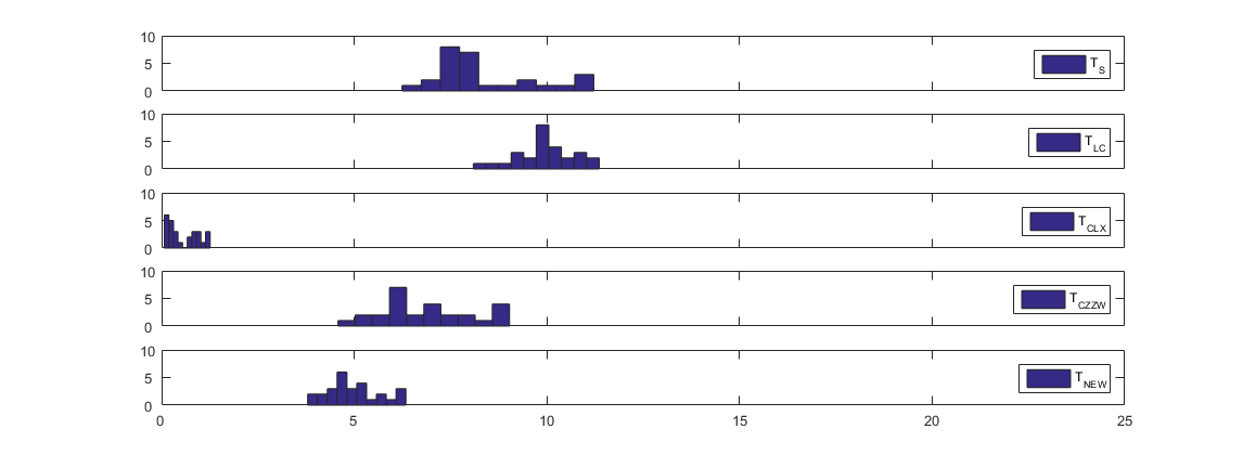
Figure 1: Histograms of the empirical sizes (in $\%$) of $T_{\mbox{\tiny S}},T_{\mbox{\tiny LC}},T_{\mbox{\tiny CLX}},T_{\mbox{\tiny CZZW}}$, and $T_{\mbox{\tiny NEW}}$ (from top to bottom) in Simulation 1. The nominal size is 5%.

To explain why $T_{\mbox{\tiny S}}$ and $T_{\mbox{\tiny LC}}$ do not perform well in terms of size control, Table 2 displays the estimated approximate degrees of freedom $\hat{d}$ (19) of $T_{\mbox{\tiny NEW}}$ under various settings in this simulation study. It is seen that the values of $\hat{d}$ all are rather small. This shows that the null distribution of $T_{\mbox{\tiny NEW}}$ is unlikely to be normal, and hence the normal approximations to the null distributions of $T_{\mbox{\tiny S}}$ and $T_{\mbox{\tiny LC}}$ are unlikely to be adequate. This partially explains why $T_{\mbox{\tiny S}}$ and $T_{\mbox{\tiny LC}}$ are not accurate in size control regardless of whether the data are less correlated ($\rho=0.25$), moderately correlated ($\rho=0.5$), or highly correlated ($\rho=0.9$). Further, it is seen that with the value of $\rho$ increasing, the value of $\hat{d}$ decreases. This means that the more highly correlated the data are, the less adequate the normal approximations to the null distributions of $T_{\mbox{\tiny S}}$ and $T_{\mbox{\tiny LC}}$ would be.

Table 2: Estimated approximate degrees of freedom of $T_{\mbox{\tiny NEW}}$ under various settings in Simulation 1.

		Model 1			Model 2			Model 3
$p$	${\bf\bm{\mathit{n}}}$	$\rho=0.25$	$\rho$ = 0.5	$\rho$ = 0.9	$\rho=0.25$	$\rho=0.5$	$\rho=0.9$	$\rho=0.25$	$\rho=0.5$	$\rho=0.9$
50	${\bf\bm{\mathit{n}}}_{1}$	2.41	1.66	1.26	3.73	2.40	1.27	4.08	1.38	1.20
	${\bf\bm{\mathit{n}}}_{2}$	2.93	1.19	1.06	3.96	1.17	1.08	3.61	1.21	1.05
	${\bf\bm{\mathit{n}}}_{3}$	2.52	1.09	1.02	1.90	1.08	1.02	2.85	1.10	1.03
100	${\bf\bm{\mathit{n}}}_{1}$	4.21	1.47	1.31	3.11	1.38	1.23	3.20	2.05	1.20
	${\bf\bm{\mathit{n}}}_{2}$	2.44	1.16	1.06	3.24	1.92	1.07	2.65	1.16	1.06
	${\bf\bm{\mathit{n}}}_{3}$	1.45	1.06	1.02	2.51	1.07	1.02	1.94	1.08	1.02
500	${\bf\bm{\mathit{n}}}_{1}$	6.85	1.40	1.23	5.97	1.72	1.37	1.95	1.51	1.24
	${\bf\bm{\mathit{n}}}_{2}$	1.86	1.09	1.05	3.23	1.09	1.05	1.61	1.09	1.05
	${\bf\bm{\mathit{n}}}_{3}$	1.36	1.04	1.03	1.45	1.04	1.03	1.29	1.05	1.02

We now compare the empirical powers of $T_{\mbox{\tiny S}}$, $T_{\mbox{\tiny LC}}$, $T_{\mbox{\tiny CLX}}$, $T_{\mbox{\tiny CZZW}}$, and $T_{\mbox{\tiny NEW}}$. Table 3 presents the empirical powers of the five tests under various configurations in Simulation 1. It is seen that the empirical powers of the five tests when $\rho_{1}=\rho_{2}=0.5$ are generally smaller than their empirical powers when $\rho_{1}\neq\rho_{2}$. This is not a surprise since in this case, the differences between ${\bf\bm{\mathit{\Sigma}}}_{1}-{\bf\bm{\mathit{\Sigma}}}_{2}$ just come from the differences between $\sigma_{1k}$’s and $\sigma_{2k}$’s. Notice also that the empirical sizes of the tests have strong impact on their empirical powers. Usually when the empirical size of a test is larger than that of another test under a setting, its empirical power is often also larger than that of another test. From Table 3, we can see that the empirical powers of $T_{\mbox{\tiny S}},T_{\mbox{\tiny LC}},$ and $T_{\mbox{\tiny CZZW}}$ are generally “larger” than those of $T_{\mbox{\tiny NEW}}$ and the empirical powers of $T_{\mbox{\tiny CLX}}$ are generally “smaller” than those of $T_{\mbox{\tiny NEW}}$. This is because from Table 1 and Figure 1, we can see that $T_{\mbox{\tiny S}},T_{\mbox{\tiny LC}},$ and $T_{\mbox{\tiny CZZW}}$ are generally more liberal than $T_{\mbox{\tiny NEW}}$, $T_{\mbox{\tiny CLX}}$ is more conservative than $T_{\mbox{\tiny NEW}}$, while $T_{\mbox{\tiny NEW}}$ has much better size control than the other tests. Therefore, when a test does not have a good size control, its empirical powers can be misleading and hence it is very important to make a test have a good size control.

Table 3: Empirical power (in $\%$) of $T_{\mbox{\tiny S}},T_{\mbox{\tiny LC}},T_{\mbox{\tiny CLX}},T_{\mbox{\tiny CZZW}}$, and $T_{\mbox{\tiny NEW}}$ in Simulation 1.

			$(\rho_{1},\rho_{2})=(0.5,0.5)$					$(\rho_{1},\rho_{2})=(0.5,0.25)$					$(\rho_{1},\rho_{2})=(0.5,0.9)$
Model	$p$	${\bf\bm{\mathit{n}}}$	$T_{\mbox{\tiny S}}$	$T_{\mbox{\tiny LC}}$	$T_{\mbox{\tiny CLX}}$	$T_{\mbox{\tiny CZZW}}$	$T_{\mbox{\tiny NEW}}$	$T_{\mbox{\tiny S}}$	$T_{\mbox{\tiny LC}}$	$T_{\mbox{\tiny CLX}}$	$T_{\mbox{\tiny CZZW}}$	$T_{\mbox{\tiny NEW}}$	$T_{\mbox{\tiny S}}$	$T_{\mbox{\tiny LC}}$	$T_{\mbox{\tiny CLX}}$	$T_{\mbox{\tiny CZZW}}$	$T_{\mbox{\tiny NEW}}$
1	50	${\bf\bm{\mathit{n}}}_{1}$	8.30	9.54	4.37	9.34	4.31	80.69	82.17	34.40	50.61	63.88	71.51	74.46	61.83	85.47	66.95
		${\bf\bm{\mathit{n}}}_{2}$	9.73	11.86	5.45	10.12	6.60	94.62	95.64	61.44	73.21	87.91	87.03	89.00	78.53	93.26	82.85
		${\bf\bm{\mathit{n}}}_{3}$	12.59	15.81	7.76	15.31	7.24	100.00	100.00	99.14	99.54	100.00	99.77	99.74	100.00	100.00	99.62
	100	${\bf\bm{\mathit{n}}}_{1}$	8.69	10.20	4.95	11.51	5.45	82.53	85.38	38.21	55.87	66.69	72.57	75.84	66.16	89.64	68.63
		${\bf\bm{\mathit{n}}}_{2}$	9.22	11.61	4.47	10.58	5.42	93.56	94.46	60.70	75.16	87.30	87.92	89.58	80.41	95.94	84.84
		${\bf\bm{\mathit{n}}}_{3}$	11.82	13.28	6.78	16.96	6.48	99.96	99.97	98.73	99.55	99.93	100.00	100.00	99.94	100.00	99.98
	500	${\bf\bm{\mathit{n}}}_{1}$	9.92	11.92	5.67	16.66	7.02	80.79	82.73	37.09	60.60	64.27	71.13	74.88	62.24	93.10	68.28
		${\bf\bm{\mathit{n}}}_{2}$	9.75	12.30	4.38	14.88	6.09	95.26	96.57	62.83	82.32	88.93	91.03	91.94	81.67	97.73	87.00
		${\bf\bm{\mathit{n}}}_{3}$	11.99	14.13	7.17	21.34	6.79	100.00	100.00	99.80	100.00	100.00	99.97	99.79	100.00	100.00	99.90
2	50	${\bf\bm{\mathit{n}}}_{1}$	9.45	10.43	3.68	7.79	5.64	81.02	81.27	33.00	47.94	59.38	71.06	72.93	55.00	83.73	63.02
		${\bf\bm{\mathit{n}}}_{2}$	12.30	13.08	3.84	9.14	6.83	94.38	94.64	54.83	68.94	83.95	87.78	88.33	77.52	92.21	82.50
		${\bf\bm{\mathit{n}}}_{3}$	15.78	16.83	6.75	14.19	7.56	100.00	99.92	98.24	99.18	99.92	99.70	99.82	99.30	99.90	99.21
	100	${\bf\bm{\mathit{n}}}_{1}$	10.34	11.24	3.30	9.50	5.06	82.38	83.13	35.49	51.66	65.47	68.50	72.37	55.66	85.80	64.26
		${\bf\bm{\mathit{n}}}_{2}$	9.91	11.22	4.02	9.01	5.54	95.96	96.07	61.08	75.18	87.43	87.59	89.40	75.17	94.24	82.74
		${\bf\bm{\mathit{n}}}_{3}$	12.06	14.83	6.00	14.68	7.19	99.95	99.92	98.67	99.43	99.89	99.84	99.81	99.45	99.93	99.55
	500	${\bf\bm{\mathit{n}}}_{1}$	8.79	10.84	3.92	12.89	6.06	85.27	86.48	31.45	57.33	68.16	70.60	74.25	53.61	89.15	66.48
		${\bf\bm{\mathit{n}}}_{2}$	11.09	12.45	2.86	9.94	6.07	96.12	96.87	63.04	81.11	90.84	88.73	90.11	75.46	95.13	85.33
		${\bf\bm{\mathit{n}}}_{3}$	12.85	15.94	5.81	20.98	6.99	100.00	100.00	98.67	99.33	99.92	100.00	100.00	100.00	100.00	100.00
3	50	${\bf\bm{\mathit{n}}}_{1}$	11.58	10.26	2.76	6.62	4.87	82.01	79.00	35.85	52.51	53.23	72.93	73.98	51.55	79.24	63.77
		${\bf\bm{\mathit{n}}}_{2}$	14.83	14.05	3.15	7.91	6.06	94.94	93.32	63.50	77.46	81.56	89.10	89.56	73.63	93.13	81.01
		${\bf\bm{\mathit{n}}}_{3}$	16.08	15.52	4.65	12.90	7.07	100.00	100.00	98.43	99.40	99.71	99.83	99.81	99.54	99.94	99.35
	100	${\bf\bm{\mathit{n}}}_{1}$	12.21	12.13	3.17	9.23	7.21	82.56	82.29	32.65	51.66	59.68	73.08	76.39	53.31	83.43	69.29
		${\bf\bm{\mathit{n}}}_{2}$	13.25	12.75	2.66	7.13	5.94	95.35	94.93	61.27	77.40	84.86	89.02	89.80	72.61	93.25	83.22
		${\bf\bm{\mathit{n}}}_{3}$	13.84	14.12	4.96	10.53	6.07	99.93	99.97	99.39	99.50	99.67	99.88	99.80	99.67	99.97	99.50
	500	${\bf\bm{\mathit{n}}}_{1}$	9.83	11.58	1.86	7.54	6.48	82.48	83.35	26.46	52.44	65.87	71.09	74.06	43.30	85.47	67.67
		${\bf\bm{\mathit{n}}}_{2}$	11.06	13.34	2.02	9.15	6.31	95.19	95.00	55.77	78.84	88.55	88.29	89.64	64.20	94.13	84.63
		${\bf\bm{\mathit{n}}}_{3}$	13.14	15.07	4.47	16.33	7.33	100.00	100.00	99.28	99.95	100.00	100.00	100.00	99.89	100.00	99.91

3.2 Simulation 2

In this simulation study, we continue to compare $T_{\mbox{\tiny NEW}}$ against $T_{\mbox{\tiny S}}$, $T_{\mbox{\tiny LC}}$, $T_{\mbox{\tiny CLX}}$, and $T_{\mbox{\tiny CZZW}}$ for the two-sample equal-covariance matrix testing problem (2) but with the two samples (1) generated from the following moving average model:

$$y_{ijk}=z_{ijk}+\theta_{i1}z_{ij(k+1)}+\cdots+\theta_{im_{i}}z_{ij(k+m_{i})},k=1,...,p;\;j=1,...,n_{i};\;i=1,2,$$

where $y_{ijk}$ denotes the $k$th component of ${\bf\bm{\mathit{y}}}_{ij}$, and $z_{ij\ell},\ell=1,\ldots,p+m_{i};\;i=1,2$ are i.i.d. random variables generated in the same way as described in Simulation 1. The covariance matrix difference ${\bf\bm{\mathit{\Sigma}}}_{1}-{\bf\bm{\mathit{\Sigma}}}_{2}$ is then determined by $m_{i},i=1,2$ and $\theta_{ij},j=1,\ldots,m_{i};\;i=1,2$. When $m_{1}=m_{2}=m$ and $\theta_{1j}=\theta_{2j}=\theta_{j},j=1,\ldots,m$, we have ${\bf\bm{\mathit{\Sigma}}}_{1}={\bf\bm{\mathit{\Sigma}}}_{2}$ so that the generated two samples (1) satisfy the null hypothesis in (2). For size comparison, we set $m=0.5p$, and let $\theta_{j},j=1,\ldots,m$ be generated from $U[2,3]$, the uniform distribution over $[2,3]$. For power comparison, we set $m_{1}=0.5p$, $m_{2}=0.4p$ and let $\theta_{1j},j=1,\ldots,m_{1}$ be generated from $U[2,3]$, and $\theta_{2j},j=1,\ldots,m_{2}$ be generated from $U[3,4]$. The tuning parameters $p$ and ${\bf\bm{\mathit{n}}}$ are specified in the same way as in Simulation 1.

Table 4 displays the empirical sizes and powers of $T_{\mbox{\tiny S}}$, $T_{\mbox{\tiny LC}}$, $T_{\mbox{\tiny CLX}}$, $T_{\mbox{\tiny CZZW}}$, and $T_{\mbox{\tiny NEW}}$ in this simulation study. In terms of size control, it is seen that the conclusions drawn from this table and Figure 2 are similar to those drawn from Table 1 and Figure 1. That is, $T_{\mbox{\tiny NEW}}$ performs well with its empirical sizes ranging from $3.79\%$ to $6.34\%$. It performs much better than $T_{\mbox{\tiny S}},T_{\mbox{\tiny LC}}$, and $T_{\mbox{\tiny CZZW}}$ which are generally quite liberal with their empirical sizes ranging from $6.24\%$ to $11.22\%$, $8.09\%$ to $11.36\%$, and $4.58\%$ to $9.03\%$, respectively. It also performs much better than $T_{\mbox{\tiny CLX}}$ which is generally quite conservative with their empirical sizes ranging from $0.07\%$ to $1.26\%$. These conclusions are also indicated by the ARE values of $T_{\mbox{\tiny S}}$, $T_{\mbox{\tiny LC}}$, $T_{\mbox{\tiny CLX}}$, $T_{\mbox{\tiny CZZW}}$, and $T_{\mbox{\tiny NEW}}$ as listed in the last row of the table. In terms of powers, it is seen that the conclusions drawn from this table are similar to those drawn from Table 3. That is, the empirical powers of $T_{\mbox{\tiny S}},T_{\mbox{\tiny LC}},$ and $T_{\mbox{\tiny CZZW}}$ are generally “larger” than those of $T_{\mbox{\tiny NEW}}$ while the empirical powers of $T_{\mbox{\tiny CLX}}$ are generally “smaller” than those of $T_{\mbox{\tiny NEW}}$. This is also because from Table 4 and Figure 2, we can see that $T_{\mbox{\tiny S}},T_{\mbox{\tiny LC}},$ and $T_{\mbox{\tiny CZZW}}$ are generally more liberal than $T_{\mbox{\tiny NEW}}$, $T_{\mbox{\tiny CLX}}$ is more conservative than $T_{\mbox{\tiny NEW}}$, while $T_{\mbox{\tiny NEW}}$ has much better size control than the other tests.

Table 4: Empirical sizes and powers (in $\%$) of $T_{\mbox{\tiny S}}$, $T_{\mbox{\tiny LC}}$, $T_{\mbox{\tiny CLX}}$, $T_{\mbox{\tiny CZZW}}$, and $T_{\mbox{\tiny NEW}}$ in Simulation 2.

			${\bf\bm{\mathit{\Sigma}}}_{1}={\bf\bm{\mathit{\Sigma}}}_{2}$					${\bf\bm{\mathit{\Sigma}}}_{1}\neq{\bf\bm{\mathit{\Sigma}}}_{2}$
Model	$p$	${\bf\bm{\mathit{n}}}$	$T_{\mbox{\tiny S}}$	$T_{\mbox{\tiny LC}}$	$T_{\mbox{\tiny CLX}}$	$T_{\mbox{\tiny CZZW}}$	$T_{\mbox{\tiny NEW}}$	$T_{\mbox{\tiny S}}$	$T_{\mbox{\tiny LC}}$	$T_{\mbox{\tiny CLX}}$	$T_{\mbox{\tiny CZZW}}$	$T_{\mbox{\tiny NEW}}$
1	50	${\bf\bm{\mathit{n}}}_{1}$	6.76	9.86	1.26	8.60	5.55	38.93	46.50	15.34	45.35	38.12
		${\bf\bm{\mathit{n}}}_{2}$	7.76	9.44	1.14	7.75	6.14	59.79	65.95	28.78	66.16	57.30
		${\bf\bm{\mathit{n}}}_{3}$	7.60	10.14	1.01	5.47	4.87	99.01	99.55	88.36	99.17	98.10
	100	${\bf\bm{\mathit{n}}}_{1}$	7.57	9.78	0.84	7.63	5.65	46.33	53.59	13.86	52.67	45.63
		${\bf\bm{\mathit{n}}}_{2}$	7.49	9.77	0.91	7.92	5.28	70.93	77.50	29.25	74.45	67.84
		${\bf\bm{\mathit{n}}}_{3}$	7.25	9.47	0.30	5.24	3.97	99.50	99.80	91.19	99.60	99.16
	500	${\bf\bm{\mathit{n}}}_{1}$	8.20	10.74	0.28	7.04	6.10	52.62	60.63	5.00	54.82	51.83
		${\bf\bm{\mathit{n}}}_{2}$	7.29	9.21	0.07	6.58	5.03	77.39	82.67	11.38	75.73	75.27
		${\bf\bm{\mathit{n}}}_{3}$	7.41	9.75	0.16	6.50	4.66	100.00	100.00	76.76	99.96	100.00
2	50	${\bf\bm{\mathit{n}}}_{1}$	10.64	10.53	0.84	8.61	6.34	40.50	44.47	12.95	43.40	32.92
		${\bf\bm{\mathit{n}}}_{2}$	9.74	11.13	0.76	6.16	4.64	64.13	67.36	25.37	60.61	54.18
		${\bf\bm{\mathit{n}}}_{3}$	9.44	10.68	0.95	6.11	5.26	98.33	98.58	82.20	97.41	96.40
	100	${\bf\bm{\mathit{n}}}_{1}$	7.72	9.73	0.79	8.29	4.91	48.43	53.99	13.06	50.41	44.22
		${\bf\bm{\mathit{n}}}_{2}$	8.05	9.36	0.29	5.97	4.30	71.25	75.87	26.28	70.24	65.42
		${\bf\bm{\mathit{n}}}_{3}$	7.84	9.96	0.35	7.19	4.67	99.71	99.83	87.26	99.19	99.20
	500	${\bf\bm{\mathit{n}}}_{1}$	7.85	9.01	0.25	9.03	5.14	50.23	56.16	3.54	53.56	47.83
		${\bf\bm{\mathit{n}}}_{2}$	6.24	8.09	0.10	6.19	3.79	77.64	82.90	11.27	76.49	74.47
		${\bf\bm{\mathit{n}}}_{3}$	7.93	10.23	0.12	6.15	5.64	100.00	100.00	77.90	100.00	100.00
3	50	${\bf\bm{\mathit{n}}}_{1}$	11.22	10.92	1.16	6.99	4.11	44.28	44.41	11.51	39.56	31.00
		${\bf\bm{\mathit{n}}}_{2}$	11.19	11.36	1.17	7.52	4.41	63.34	63.07	22.38	53.08	48.00
		${\bf\bm{\mathit{n}}}_{3}$	11.09	10.30	0.73	4.58	4.65	98.35	98.24	75.27	95.16	93.55
	100	${\bf\bm{\mathit{n}}}_{1}$	7.26	8.48	0.33	7.13	4.41	51.38	54.85	10.60	50.17	44.30
		${\bf\bm{\mathit{n}}}_{2}$	8.77	9.77	0.47	5.80	4.79	73.18	76.68	21.58	68.52	63.70
		${\bf\bm{\mathit{n}}}_{3}$	9.38	11.02	0.33	5.71	4.76	99.40	99.65	84.22	98.60	98.15
	500	${\bf\bm{\mathit{n}}}_{1}$	8.50	10.13	0.16	8.64	6.03	51.62	57.00	5.14	54.11	48.73
		${\bf\bm{\mathit{n}}}_{2}$	7.04	9.26	0.28	6.01	4.34	77.63	81.95	12.46	76.24	74.44
		${\bf\bm{\mathit{n}}}_{3}$	7.96	9.92	0.13	6.22	5.13	99.70	99.86	76.31	99.52	99.50
ARE			66.81	98.55	88.76	37.68	11.12

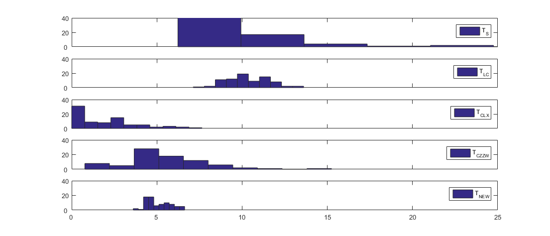
Figure 2: Histograms of the empirical sizes (in $\%$) of $T_{\mbox{\tiny S}},T_{\mbox{\tiny LC}},T_{\mbox{\tiny CLX}},T_{\mbox{\tiny CZZW}}$, and $T_{\mbox{\tiny NEW}}$ (from top to bottom) in Simulation 2.

4 Application to the Financial Data

In this section, we apply $T_{\mbox{\tiny NEW}}$, together with the other four tests, i.e., $T_{\mbox{\tiny S}}$, $T_{\mbox{\tiny LC}}$, $T_{\mbox{\tiny CLX}}$, and $T_{\mbox{\tiny CZZW}}$ to the financial data set briefly described in Section 1. It contains the daily PD of $235$ companies from the mainland of China (PD-CHN) and $153$ companies from Hong Kong (PD-HKG) in 2007–2008. We aim to check whether PD-CHN and PD-HKG have the same covariance matrix.

Table 5: Testing the equality of covariance matrices of the financial data

Hypothesis	Method	Statistic	$p$-value	d.f.
PD-CHN vs. PD-HKG	$T_{\mbox{\tiny S}}$	43.33	0
	$T_{\mbox{\tiny LC}}$	35.00	0
	$T_{\mbox{\tiny CLX}}$	34.21	$8.12\times 10^{-4}$
	$T_{\mbox{\tiny CZZW}}$	5.85	0
	$T_{\mbox{\tiny NEW}}$	11.11	$3.65\times 10^{-5}$	1.07

Table 5 presents the testing results of applying the five considered tests to the financial data set. It is seen that the $p$-values of the five tests are essentially 0, suggesting that the covariance matrices for these two groups are significantly different. In addition, the estimated approximate degrees of freedom (d.f.) of $T_{\mbox{\tiny NEW}}$ is around $1$, showing that the normal approximations to the null distributions of $T_{\mbox{\tiny S}}$ and $T_{\mbox{\tiny LC}}$ are unlikely to be adequate.

To further demonstrate the finite-sample performance of $T_{\mbox{\tiny NEW}}$ in terms of accuracy, we use the data set to calculate the empirical sizes of the five tests under consideration for PD-CHN and PD-HKG, respectively. The empirical sizes are obtained from $10,000$ runs. In each run, for PD-CHN, we randomly split the $235$ companies into two subgroups, namely PD-CHN-1 and PD-CHN-2, with their sample sizes being 117 and 118, respectively. We then compute the $p$-values of the five tests to check the equality of covariance matrices between PD-CHN-1 and PD-CHN-2. The empirical size is calculated as the proportion of times that the $p$-values are smaller than the nominal level $\alpha=5\%$ based on the $10,000$ simulation runs. Similarly, for PD-HKG, in each run, we randomly split the $153$ companies into two subgroups, namely PD-HKG-1 and PD-HKG-2, with their sample sizes being 76 and 77, respectively. Then we compute the $p$-values of the five tests to check the equality of covariance matrices between PD-HKG-1 and PD-HKG-2, and compute the empirical sizes of the five considered tests. The empirical sizes of $T_{\mbox{\tiny S}}$, $T_{\mbox{\tiny LC}}$, $T_{\mbox{\tiny CLX}}$, $T_{\mbox{\tiny CZZW}}$, and $T_{\mbox{\tiny NEW}}$ are presented in Table 6. From this table, we can see that $T_{\mbox{\tiny NEW}}$ has a much better level accuracy than the other four tests. Conclusions from the above two small-scale simulation studies based on the financial data are consistent with those drawn from the two simulation studies presented in Section 3.

Table 6: Empirical sizes ($\%$) of the financial data

Population	$T_{\mbox{\tiny S}}$	$T_{\mbox{\tiny LC}}$	$T_{\mbox{\tiny CLX}}$	$T_{\mbox{\tiny CZZW}}$	$T_{\mbox{\tiny NEW}}$
PD-CHN	24.79	13.89	0.00	7.72	6.10
PD-HKG	15.54	14.57	0.00	5.71	5.48

5 Concluding Remarks

It is often of interest to test whether two high-dimensional samples have the same covariance matrix. Existing tests are either too liberal or too conservative in terms of size control. In this paper, we propose and study a normal-reference test which has much better size control than several existing competitors as demonstrated by two simulation studies and a real data example.

In theoretical development, we assume that the mean vectors are zero to construct the test statistic while in the implementation of the proposed test, we actually replace the original two samples with the two samples obtained after subtracting the sample mean vectors. In the settings of our two simulation studies, it seems that the effect of this replacement is ignorable. However, it is still unclear if this replacement may strongly affect the performance of the proposed test in other settings. Further study in this direction is interesting and warranted.

In the implementation of the proposed test, we estimate the key quantities $\mathcal{K}_{2}(T_{n,p,0}^{*})$ and $\mathcal{K}_{3}(T_{n,p,0}^{*})$ via estimating $\operatorname{tr}({\bf\bm{\mathit{\Omega}}}_{1}^{2}),\operatorname{tr}({\bf\bm{\mathit{\Omega}}}_{1}{\bf\bm{\mathit{\Omega}}}_{2}),\operatorname{tr}({\bf\bm{\mathit{\Omega}}}_{2}^{2}),\operatorname{tr}({\bf\bm{\mathit{\Omega}}}_{1}^{3}),\operatorname{tr}({\bf\bm{\mathit{\Omega}}}_{2}^{3}),\operatorname{tr}({\bf\bm{\mathit{\Omega}}}_{1}^{2}{\bf\bm{\mathit{\Omega}}}_{2})$, and $\operatorname{tr}({\bf\bm{\mathit{\Omega}}}_{1}{\bf\bm{\mathit{\Omega}}}_{2}^{2})$, using the two induced samples (4). Whereas, it is also possible to estimate $\operatorname{tr}({\bf\bm{\mathit{\Omega}}}_{1}^{2}),\operatorname{tr}({\bf\bm{\mathit{\Omega}}}_{2}^{2})$, $\operatorname{tr}({\bf\bm{\mathit{\Omega}}}_{1}{\bf\bm{\mathit{\Omega}}}_{2}),\operatorname{tr}({\bf\bm{\mathit{\Omega}}}_{1}^{3}),\operatorname{tr}({\bf\bm{\mathit{\Omega}}}_{1}^{2}{\bf\bm{\mathit{\Omega}}}_{2}),\operatorname{tr}({\bf\bm{\mathit{\Omega}}}_{1}{\bf\bm{\mathit{\Omega}}}_{2}^{2})$, and $\operatorname{tr}({\bf\bm{\mathit{\Omega}}}_{2}^{3})$ using the original two samples (1). It is of interest to know which approach is better. Further study in this direction is interesting and warranted.

Funding and Acknowledgement

The work was financially supported by the National University of Singapore academic research grant R-155-000-121-114.

APPENDIX: Technical Proofs

Proof of Theorem 1. Notice that we can write $\tilde{T}_{n,p,0}$ and $\tilde{T}_{n,p,0}^{*}$ as generalized quadratic forms as defined in Wang and Xu, (2022, Section S.2 of the Appendix):

$$\tilde{T}_{n,p,0}=\sum_{1\leq k<l\leq n}a_{kl}{\bf\bm{\mathit{\xi}}}_{k}^{\top}{\bf\bm{\mathit{\xi}}}_{l},\quad\mbox{ and }\quad\tilde{T}_{n,p,0}^{*}=\sum_{1\leq k<l\leq n}a_{kl}{\bf\bm{\mathit{\xi}}}_{k}^{*\top}{\bf\bm{\mathit{\xi}}}_{l}^{*},$$

where ${\bf\bm{\mathit{\xi}}}_{k}={\bf\bm{\mathit{u}}}_{1k},{\bf\bm{\mathit{\xi}}}_{k}^{*}={\bf\bm{\mathit{u}}}_{1k}^{*},k=1,\ldots,n_{1}$, ${\bf\bm{\mathit{\xi}}}_{n_{1}+k}={\bf\bm{\mathit{u}}}_{2k},{\bf\bm{\mathit{\xi}}}_{n_{1}+k}^{*}={\bf\bm{\mathit{u}}}_{2k}^{*},k=1,\ldots,n_{2}$, and

$$a_{kl}=\left\{\begin{array}[]{ll}\frac{2}{n_{1}(n_{1}-1)\sigma_{T}},&\mbox{when $1\leq k<l\leq n_{1}$},\\ \frac{2}{n_{2}(n_{2}-1)\sigma_{T}},&\mbox{when $n_{1}+1\leq k<l\leq n$},\\ -\frac{2}{n_{1}n_{2}\sigma_{T}},&\mbox{when $1\leq k\leq n_{1},n_{1}+1\leq l\leq n$}.\end{array}\right.$$

We will employ Theorem S.1 of Wang and Xu, (2022) in the following proofs. To employ Theorem S.1 of Wang and Xu, (2022), we need to check Assumptions S.1 and S.2 of Wang and Xu, (2022) first. Note that we have $\sigma_{kl}^{2}=\operatorname{E}\left(a_{kl}{\bf\bm{\mathit{\xi}}}_{k}^{\top}{\bf\bm{\mathit{\xi}}}_{l}\right)^{2}=a_{kl}^{2}\operatorname{tr}({\bf\bm{\mathit{\Omega}}}_{k}{\bf\bm{\mathit{\Omega}}}_{l}),1\leq k<l\leq n$ where ${\bf\bm{\mathit{\Omega}}}_{k}={\bf\bm{\mathit{\Omega}}}_{1}$ when $1\leq k\leq n_{1}$, and ${\bf\bm{\mathit{\Omega}}}_{k}={\bf\bm{\mathit{\Omega}}}_{2}$ when $n_{1}+1\leq k\leq n$. Under Condition C2, we have

$$\begin{split}\operatorname{E}\left(a_{kl}{\bf\bm{\mathit{\xi}}}_{k}^{\top}{\bf\bm{\mathit{\xi}}}_{l}\right)^{4}&=a_{kl}^{4}\operatorname{E}({\bf\bm{\mathit{\xi}}}_{k}^{\top}{\bf\bm{\mathit{\xi}}}_{l})^{4}=a_{kl}^{4}\operatorname{E}\left[\operatorname{E}\{({\bf\bm{\mathit{\xi}}}_{k}^{\top}{\bf\bm{\mathit{\xi}}}_{l})^{4}|{\bf\bm{\mathit{\xi}}}_{k}\}\right]\\ &\leq a_{kl}^{4}\operatorname{E}\left[\gamma\operatorname{E}^{2}\{({\bf\bm{\mathit{\xi}}}_{k}^{\top}{\bf\bm{\mathit{\xi}}}_{l})^{2}|{\bf\bm{\mathit{\xi}}}_{k}\}\right]=\gamma a_{kl}^{4}\operatorname{E}\left\{({\bf\bm{\mathit{\xi}}}_{k}^{\top}{\bf\bm{\mathit{\Omega}}}_{l}{\bf\bm{\mathit{\xi}}}_{k})^{2}\right\}\\ &=\gamma a_{kl}^{4}\operatorname{E}\|{\bf\bm{\mathit{\Omega}}}_{l}^{1/2}{\bf\bm{\mathit{\xi}}}_{k}\|^{4}\leq\gamma^{2}a_{kl}^{4}\operatorname{E}^{2}(\|{\bf\bm{\mathit{\Omega}}}_{l}^{1/2}{\bf\bm{\mathit{\xi}}}_{k}\|^{2})\\ &=\gamma^{2}a_{kl}^{4}\operatorname{tr}^{2}({\bf\bm{\mathit{\Omega}}}_{k}{\bf\bm{\mathit{\Omega}}}_{l})=\gamma^{2}\sigma_{kl}^{4}.\end{split}$$

Similarly, we can show that

$$\operatorname{E}\left(a_{kl}{\bf\bm{\mathit{\xi}}}_{k}^{\top}{\bf\bm{\mathit{\xi}}}_{l}^{*}\right)^{4}\leq\gamma^{2}\sigma_{kl}^{4},\quad\operatorname{E}\left(a_{kl}{\bf\bm{\mathit{\xi}}}_{k}^{*\top}{\bf\bm{\mathit{\xi}}}_{l}\right)^{4}\leq\gamma^{2}\sigma_{kl}^{4},\quad\mbox{ and }\quad\operatorname{E}\left(a_{kl}{\bf\bm{\mathit{\xi}}}_{k}^{*\top}{\bf\bm{\mathit{\xi}}}_{l}^{*}\right)^{4}\leq\gamma^{2}\sigma_{kl}^{4}.$$

In addition, the other conditions in Assumptions S.1 and S.2 of Wang and Xu, (2022) are also satisfied by $\tilde{T}_{n,p,0}$ and $\tilde{T}_{n,p,0}^{*}$, and they are independent from each other. Applying Theorem S.1 of Wang and Xu, (2022), we have

$$\left\|\mathcal{L}(\tilde{T}_{n,p,0})-\mathcal{L}(\tilde{T}_{n,p,0}^{*})\right\|_{3}\leq\frac{\gamma^{3/2}}{3^{1/4}}\sum_{k=1}^{n}\mbox{Inf}_{k}^{3/2}.$$

By the Cauchy–Schwarz inequality, we have

$$\sum_{k=1}^{n}\mbox{Inf}_{k}^{3/2}\leq\left(\sum_{k=1}^{n}\mbox{Inf}_{k}\right)^{1/2}\left(\sum_{k=1}^{n}\mbox{Inf}_{k}^{2}\right)^{1/2}=\left\{\left(\sum_{k=1}^{n}\mbox{Inf}_{k}\right)\left(\sum_{k=1}^{n}\mbox{Inf}_{k}^{2}\right)\right\}^{1/2}.$$

Now, when $1\leq k\leq n_{1}$, by Wang and Xu, (2022, p.23 of the Appendix), we have

$$\begin{split}\mbox{Inf}_{k}&=\sum_{l=1}^{k-1}\sigma_{lk}^{2}+\sum_{l=k+1}^{n}\sigma_{kl}^{2}=\sum_{l=1}^{k-1}\sigma_{lk}^{2}+\sum_{l=k+1}^{n_{1}}\sigma_{kl}^{2}+\sum_{l=n_{1}+1}^{n}\sigma_{kl}^{2}\\ &=\sum_{l=1}^{k-1}a_{lk}^{2}\operatorname{tr}({\bf\bm{\mathit{\Omega}}}_{1}^{2})+\sum_{l=k+1}^{n_{1}}a_{kl}^{2}\operatorname{tr}({\bf\bm{\mathit{\Omega}}}_{1}^{2})+\sum_{l=n_{1}+1}^{n}a_{kl}^{2}\operatorname{tr}({\bf\bm{\mathit{\Omega}}}_{1}{\bf\bm{\mathit{\Omega}}}_{2})\\ &=\frac{4\operatorname{tr}({\bf\bm{\mathit{\Omega}}}_{1}^{2})}{n_{1}^{2}(n_{1}-1)\sigma_{T}^{2}}+\frac{4\operatorname{tr}({\bf\bm{\mathit{\Omega}}}_{1}{\bf\bm{\mathit{\Omega}}}_{2})}{n_{1}^{2}n_{2}\sigma_{T}^{2}}=\frac{2G_{1}}{n_{1}},\end{split}$$

where $G_{1}=2\{n_{1}(n_{1}-1)\}^{-1}\operatorname{tr}({\bf\bm{\mathit{\Omega}}}_{1}^{2})/\sigma_{T}^{2}+2(n_{1}n_{2})^{-1}\operatorname{tr}({\bf\bm{\mathit{\Omega}}}_{1}{\bf\bm{\mathit{\Omega}}}_{2})/\sigma_{T}^{2}$. Similarly, when $n_{1}+1\leq k\leq n$, we have $\mbox{Inf}_{k}=2G_{2}/n_{2}$ where $G_{2}=2(n_{1}n_{2})^{-1}\operatorname{tr}({\bf\bm{\mathit{\Omega}}}_{1}{\bf\bm{\mathit{\Omega}}}_{2})/\sigma_{T}^{2}+2\{n_{2}(n_{2}-1)\}^{-1}\operatorname{tr}({\bf\bm{\mathit{\Omega}}}_{2}^{2})/\sigma_{T}^{2}$. It is easy to see that $0<G_{1},G_{2}<1$ and $G_{1}+G_{2}=1$. Therefore, we have

$$\begin{split}\sum_{k=1}^{n}\mbox{Inf}_{k}&=\sum_{k=1}^{n_{1}}\mbox{Inf}_{k}+\sum_{k=n_{1}+1}^{n}\mbox{Inf}_{k}=2G_{1}+2G_{2}=2,\;\mbox{ and }\\ \sum_{k=1}^{n}\mbox{Inf}_{k}^{2}&=\sum_{k=1}^{n_{1}}\mbox{Inf}_{k}^{2}+\sum_{k=n_{1}+1}^{n}\mbox{Inf}_{k}^{2}=\frac{4G_{1}^{2}}{n_{1}}+\frac{4G_{2}^{2}}{n_{2}}\leq 4\left(\frac{1}{n_{1}}+\frac{1}{n_{2}}\right).\end{split}$$

It follows that

$$\sum_{k=1}^{n}\mbox{Inf}_{k}^{3/2}\leq 2^{3/2}\left(\frac{1}{n_{1}}+\frac{1}{n_{2}}\right)^{1/2}.$$

Thus, we have

$$\left\|\mathcal{L}(\tilde{T}_{n,p,0})-\mathcal{L}(\tilde{T}_{n,p,0}^{*})\right\|_{3}\leq\frac{(2\gamma)^{3/2}}{3^{1/4}}\left(\frac{1}{n_{1}}+\frac{1}{n_{2}}\right)^{1/2}.$$

The proof is complete.

Proof of Theorem 2. Since for $i=1,2$, we have ${\bf\bm{\mathit{u}}}_{ij}^{*},j=1,\ldots,n_{i}\stackrel{{\scriptstyle\text{i.i.d.}}}{{\sim}}N_{p^{2}}({\bf\bm{\mathit{0}}},{\bf\bm{\mathit{\Omega}}}_{i})$, then $\bar{{\bf\bm{\mathit{u}}}}_{1}^{*}-\bar{{\bf\bm{\mathit{u}}}}_{2}^{*}\sim N_{p^{2}}({\bf\bm{\mathit{0}}},{\bf\bm{\mathit{\Omega}}}_{n})$, and we can express $\|\bar{{\bf\bm{\mathit{u}}}}_{1}^{*}-\bar{{\bf\bm{\mathit{u}}}}_{2}^{*}\|^{2}={\bf\bm{\mathit{\xi}}}_{p^{2}}^{\top}{\bf\bm{\mathit{\Omega}}}_{n}{\bf\bm{\mathit{\xi}}}_{p^{2}}$, where ${\bf\bm{\mathit{\xi}}}_{p^{2}}\sim N_{p^{2}}({\bf\bm{\mathit{0}}},{\bf\bm{\mathit{I}}}_{p^{2}})$. Recall that

$$T_{n,p,0}^{*}=\|\bar{{\bf\bm{\mathit{u}}}}_{1}^{*}-\bar{{\bf\bm{\mathit{u}}}}_{2}^{*}\|^{2}-\operatorname{tr}(\hat{{\bf\bm{\mathit{\Omega}}}}_{n}^{*}),$$

where $\hat{{\bf\bm{\mathit{\Omega}}}}_{i}^{*}=(n_{i}-1)^{-1}\sum_{j=1}^{n_{i}}({\bf\bm{\mathit{u}}}_{ij}^{*}-\bar{{\bf\bm{\mathit{u}}}}_{i}^{*})({\bf\bm{\mathit{u}}}_{ij}^{*}-\bar{{\bf\bm{\mathit{u}}}}_{i}^{*})^{\top},i=1,2$, and $\hat{{\bf\bm{\mathit{\Omega}}}}_{n}^{*}=\hat{{\bf\bm{\mathit{\Omega}}}}_{1}^{*}/n_{1}+\hat{{\bf\bm{\mathit{\Omega}}}}_{2}^{*}/n_{2}$. It follows that

$$\operatorname{tr}(\hat{{\bf\bm{\mathit{\Omega}}}}_{n}^{*})=\operatorname{tr}(\hat{{\bf\bm{\mathit{\Omega}}}}_{1}^{*})/n_{1}+\operatorname{tr}(\hat{{\bf\bm{\mathit{\Omega}}}}_{2}^{*})/n_{2}.$$

Further, we have $\operatorname{E}\{\operatorname{tr}(\hat{{\bf\bm{\mathit{\Omega}}}}_{n}^{*})\}=\operatorname{tr}({\bf\bm{\mathit{\Omega}}}_{n})$ and $\operatorname{Var}\{\operatorname{tr}(\hat{{\bf\bm{\mathit{\Omega}}}}_{n}^{*})\}=2\{n_{1}^{2}(n_{1}-1)\}^{-1}\operatorname{tr}({\bf\bm{\mathit{\Omega}}}_{1}^{2})+2\{n_{2}^{2}(n_{2}-1)\}^{-1}\operatorname{tr}({\bf\bm{\mathit{\Omega}}}_{2}^{2})$. Under Condition C1, as $n\to\infty$, we have

$$\operatorname{Var}\{\operatorname{tr}(\hat{{\bf\bm{\mathit{\Omega}}}}_{n}^{*})/\operatorname{tr}({\bf\bm{\mathit{\Omega}}}_{n})\}=\frac{2\operatorname{tr}({\bf\bm{\mathit{\Omega}}}_{1}^{2})/\{n_{1}^{2}(n_{1}-1)\}+2\operatorname{tr}({\bf\bm{\mathit{\Omega}}}_{2}^{2})/\{n_{2}^{2}(n_{2}-1)\}}{\operatorname{tr}^{2}({\bf\bm{\mathit{\Omega}}}_{n})}\to 0,$$

uniformly for all $p$. Thus, $\operatorname{tr}(\hat{{\bf\bm{\mathit{\Omega}}}}_{n}^{*})/\operatorname{tr}({\bf\bm{\mathit{\Omega}}}_{n})\to 1$ in probability uniformly for all $p$. By (14), we have $\sigma_{T}^{2}=2\operatorname{tr}({\bf\bm{\mathit{\Omega}}}_{n}^{2})\{1+\lito(1)\}$. It follows that we have

$$\tilde{T}_{n,p,0}^{*}=\frac{T_{n,p,0}^{*}}{\sigma_{T}}=\frac{\|\bar{{\bf\bm{\mathit{u}}}}_{1}^{*}-\bar{{\bf\bm{\mathit{u}}}}_{2}^{*}\|^{2}-\operatorname{tr}(\hat{{\bf\bm{\mathit{\Omega}}}}_{n}^{*})}{\sqrt{\sigma_{T}^{2}}}\\ =\frac{{\bf\bm{\mathit{\xi}}}_{p^{2}}^{\top}{\bf\bm{\mathit{\Omega}}}_{n}{\bf\bm{\mathit{\xi}}}_{p^{2}}-\operatorname{tr}({\bf\bm{\mathit{\Omega}}}_{n})}{\sqrt{2\operatorname{tr}({\bf\bm{\mathit{\Omega}}}_{n}^{2})}}\{1+\lito_{p}(1)\}.$$

Under Condition C3, the expression (12) follows from Corollary 1 of Wang and Xu, (2022) immediately. The proof is complete.

Proof of Theorem 3. By (8) and under the local alternative (20), we have

$$T_{n,p}=\left[T_{n,p,0}+\operatorname{tr}\left\{({\bf\bm{\mathit{\Sigma}}}_{1}-{\bf\bm{\mathit{\Sigma}}}_{2})^{2}\right\}\right]\{1+\lito_{p}(1)\}.$$

By (10) and (21), we have $\sigma_{T}^{2}=2\operatorname{tr}({\bf\bm{\mathit{\Omega}}}_{n}^{2})\{1+\lito(1)\}=2\{n\tau(1-\tau)\}^{-2}\operatorname{tr}({\bf\bm{\mathit{\Omega}}}^{2})\{1+\lito(1)\}$. In addition, under the given conditions, we have $\hat{\beta}_{0}/\beta_{0}\stackrel{{\scriptstyle P}}{{\longrightarrow}}1,\hat{\beta}_{1}/\beta_{1}\stackrel{{\scriptstyle P}}{{\longrightarrow}}1$, and $\hat{d}/d\stackrel{{\scriptstyle P}}{{\longrightarrow}}1$ as $n,p\to\infty$. We first prove (22). Under Conditions C1–C3, Theorems 1 and 2 indicate that as $n,p\to\infty$, we have $\tilde{T}_{n,p,0}=T_{n,p,0}/\sigma_{T}\stackrel{{\scriptstyle\mathcal{L}}}{{\longrightarrow}}\zeta$ where $\zeta$ is defined in Theorem 2. It follows that as $n,p\to\infty$, we have

$$\begin{split}&\quad\Pr\left\{T_{n,p}\geq\hat{\beta}_{0}+\hat{\beta}_{1}\chi_{\hat{d}}^{2}(\alpha)\right\}\\ &=\Pr\left[\tilde{T}_{n,p,0}\geq\frac{\beta_{0}+\beta_{1}\chi^{2}_{d}(\alpha)}{\sigma_{T}}-\frac{\operatorname{tr}\left\{({\bf\bm{\mathit{\Sigma}}}_{1}-{\bf\bm{\mathit{\Sigma}}}_{2})^{2}\right\}}{\sqrt{2\{n\tau(1-\tau)\}^{-2}\operatorname{tr}({\bf\bm{\mathit{\Omega}}}^{2})}}\right]\{1+\lito(1)\}\\ &=\Pr\left[\zeta\geq\frac{\chi_{d}^{2}(\alpha)-d}{\sqrt{2d}}-\frac{n\tau(1-\tau)}{\sqrt{2\operatorname{tr}({\bf\bm{\mathit{\Omega}}}^{2})}}\operatorname{tr}\left\{({\bf\bm{\mathit{\Sigma}}}_{1}-{\bf\bm{\mathit{\Sigma}}}_{2})^{2}\right\}\right]\{1+\lito(1)\},\end{split}$$ (A.1)

where $\tau$ is defined in Condition C1.

We next prove (23). Under the given conditions, when $d\to\infty$, Theorem 2 indicates that as $n,p\to\infty$, we have $\tilde{T}_{n,p,0}\stackrel{{\scriptstyle\mathcal{L}}}{{\longrightarrow}}\zeta\sim N(0,1)$ and $\tilde{T}_{n,p,0}^{*}\stackrel{{\scriptstyle\mathcal{L}}}{{\longrightarrow}}N(0,1)$. In addition, as $d\to\infty$, we have $\{\chi_{d}^{2}(\alpha)-d\}/\sqrt{2d}\to z_{\alpha}$ where $z_{\alpha}$ denotes the upper $100\alpha$-percentile of $N(0,1)$. Then by (A.1), as $n,p\to\infty$, we have

$$\Pr\left\{T_{n,p}\geq\hat{\beta}_{0}+\hat{\beta}_{1}\chi_{\hat{d}}^{2}(\alpha)\right\}=\Phi\left[-z_{\alpha}+\frac{n\tau(1-\tau)}{\sqrt{2\operatorname{tr}({\bf\bm{\mathit{\Omega}}}^{2})}}\operatorname{tr}\left\{({\bf\bm{\mathit{\Sigma}}}_{1}-{\bf\bm{\mathit{\Sigma}}}_{2})^{2}\right\}\right]\{1+\lito(1)\},$$

where $\Phi(\cdot)$ denotes the cumulative distribution of $N(0,1)$. The proof is complete.

References

- Bai and Saranadasa, (1996) Bai, Z. D. and Saranadasa, H. (1996). Effect of high dimension: by an example of a two sample problem. Statistica Sinica, 6(2):311–329.
- Cai et al., (2013) Cai, T., Liu, W., and Xia, Y. (2013). Two-Sample Covariance Matrix Testing and Support Recovery in High-Dimensional and Sparse Settings. Journal of the American Statistical Association, 108(501):265–277.
- Chang et al., (2017) Chang, J., Zhou, W., Zhou, W.-X., and Wang, L. (2017). Comparing large covariance matrices under weak conditions on the dependence structure and its application to gene clustering. Biometrics, 73(1):31–41.
- Chen and Qin, (2010) Chen, S. X. and Qin, Y.-L. (2010). A two-sample test for high-dimensional data with applications to gene-set testing. The Annals of Statistics, 38(2):808–835.
- Duan et al., (2012) Duan, J.-C., Sun, J., and Wang, T. (2012). Multiperiod corporate default prediction—a forward intensity approach. Journal of Econometrics, 170(1):191–209.
- Hyodo et al., (2020) Hyodo, M., Nishiyama, T., and Pavlenko, T. (2020). On error bounds for high-dimensional asymptotic distribution of -type test statistic for equality of means. Statistics & Probability Letters, 157:108637.
- Li and Chen, (2012) Li, J. and Chen, S. X. (2012). Two sample tests for high-dimensional covariance matrices. The Annals of Statistics, 40(2):908 – 940.
- Schott, (2007) Schott, J. R. (2007). A test for the equality of covariance matrices when the dimension is large relative to the sample sizes. Computational Statistics & DataAnalysis, 51:6535–6542.
- Srivastava and Du, (2008) Srivastava, M. S. and Du, M. (2008). A test for the mean vector with fewer observations than the dimension. Journal of Multivariate Analysis, 99(3):386–402.
- Wang and Xu, (2022) Wang, R. and Xu, W. (2022). An approximate randomization test for the high-dimensional two-sample Behrens–Fisher problem under arbitrary covariances. Biometrika. asac014.
- Westfall, (2014) Westfall, P. H. (2014). Kurtosis as peakedness, 1905–2014. rip. The American Statistician, 68(3):191–195.
- Zhang, (2005) Zhang, J.-T. (2005). Approximate and asymptotic distributions of chi-squared-type mixtures with applications. Journal of the American Statistical Association, 100(469):273–285.
- Zhang, (2011) Zhang, J.-T. (2011). Two-way MANOVA with unequal cell sizes and unequal cell covariance matrices. Technometrics, 53(4):426–439.
- Zhang, (2013) Zhang, J.-T. (2013). Analysis of variance for functional data. CRC Press.
- (15) Zhang, J.-T., Guo, J., Zhou, B., and Cheng, M.-Y. (2020a). A simple two-sample test in high dimensions based on -norm. Journal of American Statistical Association, 115(530):1011–1027.
- Zhang et al., (2022) Zhang, J.-T., Zhou, B., and Guo, J. (2022). Testing high-dimensional mean vector with applications. Statistical Papers, 63(4):1105–1137.
- Zhang et al., (2021) Zhang, J.-T., Zhou, B., Guo, J., and Zhu, T. (2021). Two-sample behrens–fisher problems for high-dimensional data: A normal reference approach. Journal of Statistical Planning and Inference, 213:142–161.
- Zhang and Zhu, (2022) Zhang, J.-T. and Zhu, T. (2022). A further study on chen qin’s test for two-sample behrens–fisher problems for high-dimensional data. Journal of Statistical Theory and Practice, 16:1.
- (19) Zhang, L., Zhu, T., and Zhang, J.-T. (2020b). A simple scale-invariant two-sample test for high-dimensional data. Econometrics and Statistics, 14:131 – 144.