Exact solutions and conservation laws
of a one-dimensional PDE model
for a blood vessel

Abstract.

Two aspects of a widely used 1D model of blood flow in a single blood vessel are studied by symmetry analysis, where the variables in the model are the blood pressure and the cross-section area of the blood vessel. As one main result, all travelling wave solutions are found by explicit quadrature of the model. The features, behaviour, and boundary conditions for these solutions are discussed. Solutions of interest include shock waves and sharp wave-front pulses for the pressure and the blood flow. Another main result is that three new conservation laws are derived for inviscid flows. Compared to the well-known conservation laws in 1D compressible fluid flow, they describe generalized momentum and generalized axial and volumetric energies. For viscous flows, these conservation laws get replaced by conservation balance equations which contain a dissipative term proportional to the friction coefficient in the model.

1. Introduction

In recent years, one-dimensional (1D) models of blood flow in human blood vessels have been widely used in clinical applications [1, 2]. These models are effective for understanding averaged features of blood flow locally, such as velocity, volume flux, and pressure [3, 4]. They can also be combined with 3D models for detailed simulation of the human cardiovascular system as a whole [5, 6, 7]. Moreover, 1D models have much less computational cost compared to 3D models and can be mathematically analyzed in greater depth.

A non-branching blood vessel in a 1D model is a cylindrical tube whose radius varies as a function of time $t$ and axial distance $x$, in which the blood is an incompressible fluid governed by the Navier-Stokes equations averaged over cross-sections of the tube. The variables consist of the cross-section area $A$, the volume flux $Q$ of blood flow, the mean pressure $P$, and the mean blood velocity $\bar{u}=Q/A$, while the blood density is taken to be constant. $A$ and $Q$ satisfy a system of two coupled partial differential equations (PDEs) which are similar in form to the Navier-Stokes equations for mass continuity and momentum in fluid mechanics. The system is closed by specifying a relation for the pressure in terms of the cross-section area; the simplest widely-used model is that the pressure change across the vessel wall is proportional to the change in radius of the vessel. There are two important parameters in the resulting closed system: a friction parameter, which is proportional to the viscosity coefficient in the Navier-Stokes equations; and a momentum correction parameter, which arises from how the Navier-Stokes are averaged over a cross-section [8].

In the literature, there is a lot of work on numerical solutions, but very little has been done on exact solutions except for steady-states [9, 10, 11] and the use of the well-known Riemann method of characteristics for wave propagation [12, 13]. The latter method, however, can be carried out to obtain explicit solutions only in a special case for the momentum correction parameter [4].

The main purpose of the present paper is to illustrate the utility of symmetry analysis applied to a 1D model of blood flow in a single blood vessel, which will provide explicit analytical information about exact non-steady solutions and conservation laws. Two main results will be obtained.

Firstly, all explicit travelling wave solutions of the model will be derived – namely, a wave form for $A$ and $Q$ that moves with a constant speed and preserves its shape. A complete discussion of these solutions and their properties is given.

One type of solution obtained describes a dissipating shock wave in a very long constricting blood vessel with a steady-state near each end; the vessel’s diameter, pressure, and blood flow display a rapid transition in the shock, which moves at a constant speed. A similar shock wave solution is found for a blood vessel of arbitrary length in which the initial state of the blood vessel is close to a steady-state and then rapidly transitions such that the diameter, pressure, and blood flow are increasing. The blood velocity exhibits a shock behaviour between two steady-states.

Another type of solution obtained describes a pulse with a sharp front for the blood vessel’s diameter, pressure, and blood flow; behind the front, these quantities decrease to a steady-state behaviour. Other solutions are obtained that exhibit a similar sharp front, with different behaviours behind the front.

In general, solutions that describe travelling waves in an infinitely long tube can be applied to modelling a very long blood vessel where the morphology at the ends of the vessel is not relevant. When the morphology at the ends is important, an explanation will be given of how the travelling wave solutions are applicable with various boundary conditions satisfied at the end points. More discussion of the applicability of travelling waves will be given at the end of the paper.

Secondly, some explicit new conservation laws admitted by the model will be derived. The only well-known conservation laws to-date have been the total blood volume and the net blood flux, plus an Eulerian energy quantity which holds only in a special case of the momentum correction parameter [4]. Three new conservation laws are obtained: a generalized momentum and two generalized energies, which hold for any value of the momentum correction parameter and for a general pressure-area relation when the blood flow is modelled as being inviscid. The momentum quantity is a modified form of the well-known momentum in fluid mechanics. The energy quantities represent a volumetric energy and an axial energy, which are similar to generalizations of the well-known energy in fluid mechanics (for the Euler equations of inviscid flow). It is interesting, however, that there are two different conserved energies for the blood flow model. When the blood flow is modelled as being viscous, then these three new quantities are no longer conserved but they satisfy conservation balance equations that contain a dissipative volume term proportional to friction coefficient. Such balance equations are useful in mathematical analysis of the initial-value problem.

In particular, it is known that the Eulerian energy quantity satisfies a balance equation leading to a time-decay inequality [4]. This quantity coincides with the total volumetric energy in the blood flow model in a special case for the momentum correction parameter, but otherwise it is not conserved in the blood flow model even for inviscid flow. Analogous inequalities can be derived for the viscous blood flow model by use of the volumetric energy and axial energy with no restriction on the momentum correction parameter.

Furthermore, the new conservation laws yield associated boundary conditions for the model such that the flux of the generalized momentum and the generalized energies is zero in the rest frame of the blood flow. These zero-flux boundary conditions can be applied to travelling wave solutions, as well as steady-state solutions.

All of these results are new. A worthwhile remark is that the viewpoint here is applied mathematics, rather than biological modelling.

Section 2 summarizes the blood flow PDEs and various commonly used forms for the pressure-area relation. The kinematical symmetries and the five basic conservation laws of the model with a general pressure-area relation are derived.

Section 3 has a general discussion of boundary conditions for the model, including zero-flux boundary conditions coming from the three new conservation equations.

Section 4 starts with deriving the system of ordinary differential equations (ODEs) satisfied by travelling wave solutions of the blood flow PDEs. These ODEs have a quadrature which is obtained for the separate cases of inviscid and viscous flow. Spatial domains and boundary conditions for the solutions are then considered. Some main features of travelling waves are shown to hold for all pressure-area relations.

Section 5 presents all of the exact travelling wave solutions in the case of the most widely used pressure-area relation, and discusses their basic mathematical and physical features.

Section 6 makes some concluding remarks.

2. Summary and features of the 1D model

The PDE system for the quantities $A(x,t)$, $Q(x,t)$, $P(x,t)$ describing cross-section area, blood flow, and pressure in a cylindrical blood vessel is given by [8]

$$A_{t}+Q_{x}=0,$$ (1)

$$Q_{t}+\alpha(Q^{2}/A)_{x}+\rho_{0}^{-1}AP_{x}+kQ/A=0$$ (2)

where $\alpha\geq 1$ is a momentum correction coefficient (determined by the axial velocity profile), $k\geq 0$ is the friction coefficient (proportional to the viscosity). Here $\rho_{0}>0$ is the blood density, which is constant.

The pressure-area relation, which closes the system and is sometime called a “tube law”, has the general form [14]

$$P=\beta f(A/A_{0})+P_{\text{ext.}}$$ (3)

where $\beta>0$ is a constant, and $P_{\text{ext.}}$ is the external pressure caused by the tissue surrounding the blood vessel, which will be assumed to be constant. If there is no change in pressure across the vessel wall, then the blood vessel is assumed to have a constant area $A=A_{0}$, whereby $P(A_{0})=P_{\text{ext.}}$ implies that $f(1)=0$. Physiologically, it is expected that the pressure change should be an increasing positive function of the area:

$$f(A/A_{0})\geq 0\quad\text{ and }\quad f^{\prime}(A/A_{0})>0$$ (4)

for $A>0$. A variety of functional relations with these properties have been proposed in the literature, for example [4, 14, 15, 10]:

$$f =\sqrt{A/A_{0}}-1;$$ (5a)

$$f =1-1/\sqrt{A/A_{0}};$$ (5b)

$$f =\exp(A/A_{0}-1)-1;$$ (5c)

$$f =(A/A_{0})^{m}-(A/A_{0})^{n},\quad m>0\geq n.$$ (5d)

The most commonly used relation is (5a) which models the pressure change being proportional to the change in radius of the blood vessel,

$$P-P_{\text{ext.}}=\beta(\sqrt{A/A_{0}}-1).$$ (6)

For details of the derivation of this model (1), (2), (6) and further explanation of its biological and physical features, see Ref. [16, 11, 17].

Substitution of the general pressure-area relation (3) into the PDEs (1)–(2) yields the closed system

$$A_{t}+Q_{x}=0,$$ (7)

$$Q_{t}+\alpha(Q^{2}/A)_{x}+\beta_{0}(A/A_{0})f^{\prime}(A/A_{0})A_{x}+kQ/A=0$$ (8)

where $\beta_{0}=\beta/\rho_{0}>0$. In terms of $Q$ and $A$, the mean blood flow velocity is

$$\bar{u}=Q/A.$$ (9)

This system, with $A>0$, is well known to be hyperbolic, and consequently it possesses two Riemann invariants which propagate with speeds

$$c_{\pm}=\alpha\bar{u}\pm\sqrt{\beta_{0}(A/A_{0})f^{\prime}(A/A_{0})+\alpha(\alpha-1)\bar{u}^{2}}$$ (10)

(see e.g. Ref. [16]). This means that the system admits nonlinear waves that travel along the paths determined by $dx/dt=c_{\pm}$.

The most important parameter in the system (7)–(8) is the friction coefficient $k\geq 0$. In applications, there are two main cases of interest.

Viscous: $k>0$. In this case, the system (7)–(8) is dissipative. As an illustration, spatially homogeneous solutions $(A(t),Q(t))$ satisfy $A^{\prime}=0$ and $Q^{\prime}=-kQ/A$, which gives $A=A_{\text{s}}$ and $Q=Q_{0}e^{-\tfrac{k}{A_{s}}t}$, where $A_{\text{s}}$ is a positive constant and $Q_{0}$ is an arbitrary constant. These solutions describe a blood vessel with a constant radius and a blood flux that exponentially drops to zero on a time scale $A_{s}/k$.

Inviscid: $k=0$. In this case, the system (7)–(8) is non-dissipative. Spatially homogeneous solutions $(A(t),Q(t))$ simply are constants, $A=A_{\text{s}}>0$ and $Q=Q_{\text{s}}$, which describes a blood vessel with a constant radius carrying a constant blood flux.

2.1. Kinematic point symmetries

The system (7)–(8) has the following kinematic transformation groups of symmetries:

space reflection $$x\to-x,\ Q\to-Q$$ (11)

time translation $$t\to t+\epsilon$$ (12)

axial translation $$x\to x+\epsilon$$ (13)

scaling $$t\to e^{\epsilon}t,\ x\to e^{(1+\frac{q}{2})\epsilon}x,\ A\to e^{\epsilon}A,\ Q\to e^{(1+\frac{q}{2})\epsilon}Q,\quad f=(A/A_{0})^{q}-1$$ (14)

where $\epsilon$ is the parameter in the symmetry group. In the inviscid case, the system has additional kinematic symmetry transformation groups:

time reversal $$t\to-t,\ Q\to-Q$$ (15)

dilation $$t\to e^{\epsilon}t,\ x\to e^{\epsilon}x$$ (16)

Galilean boost $$x\to x+\epsilon t,\ Q\to Q+\epsilon A,\quad\alpha=1$$ (17)

Note that the Galilean boost corresponds to $\bar{u}\to\bar{u}+\epsilon$.

These symmetries (11)–(17) are evident by inspection of the form of the system (7)–(8) in comparison to the 1D Navier-Stokes equations for compressible fluids whose Lie point symmetries and discrete symmetries are well known [18, 19, 20].

A determination of all point transformation symmetries is fairly complicated and will involve utilizing the form of the Riemann invariants.

For a general discussion of symmetries and their applications to PDEs, see Ref. [18, 21, 22].

2.2. Basic conservation laws

Some conservation laws of the system (7)–(8) can be readily found by comparison with the well-known conservation laws of mass, momentum, and energy in the inviscid case, for 1D compressible fluid dynamics [18, 19, 23]. Mathematically, $A$ is analogous to mass density $\rho$, and $Q$ is analogous to the momentum density $\rho u$, where $\rho$ and $u$ are density and velocity variables in the 1D inviscid fluid equations

$$\rho_{t}+(\rho u)_{x}=0,\quad(\rho u)_{t}+(\rho u^{2}+p(\rho))_{x}=0,$$ (18)

while the fluid pressure $p(\rho)$ then corresponds to $\int_{A_{0}}^{A}\beta_{0}(A/A_{0})f^{\prime}(A/A_{0})\,dA$. This analogy is exact in the case $k=0$, $\alpha=1$.

Firstly, the PDE (7) itself is a continuity equation for $A$ viewed as a density. Integration of $A$ over any portion $x_{1}\leq x\leq x_{2}$ of a blood vessel gives the total volume of blood in that portion:

$$V=\int_{x_{1}}^{x_{2}}A\,dx.$$ (19)

This quantity satisfies the conservation law

$$\tfrac{d}{dt}V=-Q\big{|}_{x_{1}}^{x_{2}}$$ (20)

stating that the rate of change in blood volume is balanced by the net change in blood flow through the end points $x=x_{1}$ and $x=x_{2}$. The analogous conservation law in 1D fluid dynamics is the mass.

Likewise, the PDE (8) in the inviscid case, $k=0$, is a continuity equation for $Q$ viewed as a density. The integral of $\tfrac{1}{L}Q$ over $x_{1}\leq x\leq x_{2}$, with $L=x_{2}-x_{1}$, gives the net (mean) blood flux

$$\bar{Q}=\tfrac{1}{L}\int_{x_{1}}^{x_{2}}Q\,dx$$ (21)

which satisfies the conservation law

$$\tfrac{d}{dt}\bar{Q}=-\tfrac{1}{L}\big{(}\alpha Q^{2}/A+\beta_{0}\big{(}Af(A/A_{0})-F(A)\big{)}\big{)}\big{|}_{x_{1}}^{x_{2}}=-\tfrac{2}{L}\rho_{0}^{-1}{\bar{P}}A\big{|}_{x_{1}}^{x_{2}}$$ (22)

with $F(A)=\int_{A_{0}}^{A}f(A/A_{0})\,dA$, where

$$\bar{P}=\tfrac{1}{2}\alpha\rho_{0}{\bar{u}}^{2}+\tfrac{1}{2}\big{(}P(A)-\beta A^{-1}F(A)-P_{\text{ext.}}\big{)}$$ (23)

is the analog of mechanical pressure in inviscid constant-density fluid dynamics [24]. Thus, the rate of change in the net blood flux is proportional to the difference in the mechanical force ${\bar{P}}A$ on the cross-sections at each end. In the case of viscous blood flow, the conservation law is replaced by a balance equation

$$\tfrac{d}{dt}\bar{Q}=-\tfrac{2}{L}\rho_{0}^{-1}{\bar{P}}A\big{|}_{x_{1}}^{x_{2}}-k\bar{U}$$ (24)

where $\bar{U}=\tfrac{1}{L}\int_{x_{1}}^{x_{2}}\bar{u}\,dx$ is mean velocity. This is analogous to the momentum balance equation in 1D viscous fluid dynamics.

Secondly, through the analogy mentioned earlier, energy in 1D inviscid fluid dynamics corresponds to the quantity [4] $E=\int_{x_{1}}^{x_{2}}(\tfrac{1}{2}Q^{2}/A+\beta_{0}F(A))\,dx$, which satisfies $\tfrac{d}{dt}E=-\big{(}Q^{3}/A^{2}+\beta_{0}Qf(A/A_{0})\big{|}_{x_{1}}^{x_{2}}$ when $\alpha=1$ and $k=0$. This energy balance equation can be derived directly from the summed product of the PDEs (7)–(8) and the pair of expressions $\big{(}{-\tfrac{1}{2}}Q^{2}/A^{2}+\beta_{0}A^{2}f(A/A_{0}),Q/A\big{)}$, called a multiplier.

A generalized energy can be sought for $\alpha\neq 1$ by adjusting the multiplier using a suitable power of $A$. Specifically, the adjusted multiplier $\big{(}({-\tfrac{r}{2}}Q^{2}+h(A))A^{-1-r},QA^{-r}\big{)}$ with a suitable choice of $h(A)$ leads to the balance equation

$$\big{(}\tfrac{1}{2}Q^{2}A^{-r}+\beta_{0}J(A;r)\big{)}_{t}+\big{(}\tfrac{4\alpha-r}{6}Q^{3}A^{-r-1}+\beta_{0}QJ(A;r)\big{)}_{x}=-kQ^{2}A^{-r-1}$$ (25)

with

$$J(A;r)=AH(A;r)+(r-2)\int_{A_{0}}^{A}H(A;r)\,dA,\quad H(A;r)=\int_{A_{0}}^{A}A^{-r}f(A/A_{0})\,dA,$$ (26)

where $r^{2}-(4\alpha-1)r+2\alpha=0$. The roots

$$r_{\pm}=2\alpha-\tfrac{1}{2}\pm 2\sqrt{\alpha(\alpha-1)+\tfrac{1}{16}}$$ (27)

are real and satisfy $r_{+}\geq 2$, $1\geq r_{-}>\tfrac{1}{2}$ since $\alpha\geq 1$. In the inviscid case, $k=0$, integration of the density term in the balance equation (25) times $\rho_{0}$ gives the integral quantities

$$E^{\pm}=\int_{x_{1}}^{x_{2}}\big{(}\tfrac{1}{2}\rho_{0}Q^{2}/A^{r_{\pm}}+\beta J(A;r_{\pm})\big{)}\,dx$$ (28)

which satisfy the conservation laws

$$\tfrac{d}{dt}E^{\pm}=-\big{(}\tfrac{4\alpha-r_{\pm}}{6}\rho_{0}Q^{3}/A^{r_{\pm}+1}+\beta QH(A;r_{\pm})\big{)}\big{|}_{x_{1}}^{x_{2}}.$$ (29)

In the viscous case, the righthand side of the conservation equation (29) will also contain a dissipative integral term $-k\int_{x_{1}}^{x_{2}}Q^{2}/A^{r_{\pm}+1}\,dx$.

For $\alpha=1$, note that the generalized energy integrals (28) become

$$E^{-}=\rho_{0}\int_{x_{1}}^{x_{2}}(\tfrac{1}{2}\bar{u}^{2}+\beta_{0}J^{-}(A))A\,dx=E\quad\text{ and }\quad E^{+}=\rho_{0}\int_{x_{1}}^{x_{2}}(\tfrac{1}{2}\bar{u}^{2}+\beta_{0}J^{+}(A))\,dx$$ (30)

in terms of $J^{-}(A)=J(A;r_{-})=\int_{0}^{1}f(\lambda A/A_{0})\,d\lambda$ and $J^{+}(A)=J(A;r_{+})=A\int_{A_{0}}^{A}A^{-2}f(A/A_{0})\,dA$ after simplifications, where $r_{-}=1$, $r_{+}=2$. The quantity $E^{-}$ is the volumetric energy of the blood flow, while the other quantity $E^{+}$ is the axial energy.

The same method also leads to a generalized momentum which arises from the multiplier $((1-2\alpha)QA^{-2\alpha},A^{1-2\alpha})$. This yields a balance equation

$$\big{(}QA^{1-2\alpha}\big{)}_{t}+\big{(}\tfrac{1}{2}Q^{2}A^{-2\alpha}+\beta_{0}G(A;\alpha)\big{)}_{x}=-kQA^{-2\alpha}$$ (31)

with

$$G(A;\alpha)=A^{2(1-\alpha)}f(A/A_{0})+2(\alpha-1)\int_{A_{0}}^{A}A^{1-2\alpha}f(A/A_{0})\,dA.$$ (32)

Integration of the density term times $\rho_{0}$ gives the integral quantity

$$M=\rho_{0}\int_{x_{1}}^{x_{2}}Q/A^{2\alpha-1}\,dx=\rho_{0}\int_{x_{1}}^{x_{2}}\bar{u}/A^{2(\alpha-1)}\,dx$$ (33)

satisfying

$$\tfrac{d}{dt}M=-\big{(}\tfrac{1}{2}\rho_{0}Q^{2}/A^{2\alpha}+\beta G(A;\alpha))\big{|}_{x_{1}}^{x_{2}}-k\int_{x_{1}}^{x_{2}}Q/A^{2\alpha}\,dx.$$ (34)

This conservation equation becomes a conservation law in the inviscid case, $k=0$.

For $\alpha=1$, note that the generalized momentum integral (33) reduces to $M=\rho_{0}\int_{x_{1}}^{x_{2}}\bar{u}\,dx$ which is the momentum of the blood flow. It is interesting that, in contrast to 1D fluid dynamics, the blood flow system possesses this additional conserved momentum as well as an additional conserved energy $E^{+}$.

A determination of all low-order conserved integrals and balance equations is, in principle, possible by the method of multipliers. However, similarly to the situation for symmetries, it is fairly complicated and will involve utilizing the form of the Riemann invariants.

For a general discussion of multipliers and conservation laws of PDEs, see Ref. [21, 22, 25, 26].

2.3. Conserved integrals moving with the flow

In fluid dynamics, it is useful to formulate conservation laws on domains that move with the fluid flow [19, 24]. A similar formulation can be given for the conservation equations (20), (22), (34) and (29) so that they hold on moving domains $x_{1}(t)\leq x(t)\leq x_{2}(t)$ in the blood flow, as given by

$$\frac{dx(t)}{dt}=\bar{u}(t,x(t)).$$ (35)

The moving blood volume is defined by

$$V_{\text{mov.}}=\int_{x_{1}(t)}^{x_{2}(t)}A\,dx$$ (36)

which satisfies

$$\tfrac{d}{dt}V_{\text{mov.}}=0.$$ (37)

Thus $V_{\text{mov.}}$ is a constant of motion. The moving net blood flux

$$\bar{Q}_{\text{mov.}}=\frac{1}{L(t)}\int_{x_{1}(t)}^{x_{2}(t)}Q\,dx,$$ (38)

with $L(t)=x_{2}(t)-x_{1}(t)$, satisfies the conservation law

$$\tfrac{d}{dt}\big{(}L(t)\bar{Q}_{\text{mov.}}\big{)}=-\big{(}(\alpha-1)Q^{2}/A+\beta_{0}\big{(}Af(A/A_{0})-F(A)\big{)}\big{)}\big{|}_{x_{1}(t)}^{x_{2}(t)}-kL(t)\bar{U}_{\text{mov.}}$$ (39)

where $\bar{U}_{\text{mov.}}=\tfrac{1}{L(t)}\int_{x_{1}(t)}^{x_{2}(t)}\bar{u}\,dx$ is the moving mean velocity.

In the inviscid case, the moving version of the conservation balance equations (34) and (29) take the form

$$\tfrac{d}{dt}M_{\text{mov.}}=-\big{(}\beta G(A;\alpha)-\tfrac{1}{2}\rho_{0}Q^{2}/A^{2\alpha})\big{|}_{x_{1}(t)}^{x_{2}(t)}$$ (40)

for the moving generalized momentum

$$M_{\text{mov.}}=\rho_{0}\int_{x_{1}(t)}^{x_{2}(t)}\bar{u}/A^{2(\alpha-1)}\,dx,$$ (41)

and

$$\tfrac{d}{dt}E^{\pm}_{\text{mov.}}=-\big{(}\beta QG(A;\tfrac{1}{2}r_{\pm})-\tfrac{1}{6}(r_{\pm}+3-4\alpha)\rho_{0}Q^{3}/A^{r_{\pm}+1}\big{)}\big{|}_{x_{1}(t)}^{x_{2}(t)}$$ (42)

for the moving generalized volumetric energy $(-)$ and axial energy $(+)$

$$E^{\pm}_{\text{mov.}}=\int_{x_{1}(t)}^{x_{2}(t)}\big{(}\tfrac{1}{2}\rho_{0}Q^{2}/A^{r_{\pm}}+\beta J(A;r_{\pm})\big{)}\,dx,$$ (43)

where $r_{\pm}$ is given by expression (27) in terms of $\alpha$.

3. Boundary conditions

As a model for blood flow, the system (7)–(8) must be supplemented by boundary conditions at the ends of blood vessel, $x=x_{1}$ and $x=x_{2}$, with $x_{2}>x_{1}$. Because this system is hyperbolic, a general argument based on the theory of characteristics indicates that a single boundary condition can be posed at each end [7, 27, 28]. The specific type of boundary condition involves the particular biological morphology of the ends of the blood vessel being modelled: an end that is branching; an end that terminates or is blocked; an end that is open; an end that has blood pumped in or out; an end that has a fixed diameter or a fixed pressure; an end at which a pressure wave or blood flow pulse is propagating in or out; an end with a steady-state pressure. Attention here will be restricted to the latter two cases. Note that, depending on the morphology, the two ends can have different types of boundary conditions.

Propagation of a pressure wave with speed $c$ along a blood vessel is specified by conditions $cP_{x}=P_{t}$ at each end. From the pressure-area relation (3), this is equivalent to the boundary conditions

$$cA_{x}(x_{1},t)=A_{t}(x_{1},t),\quad cA_{x}(x_{2},t)=A_{t}(x_{2},t),\quad t\geq 0.$$ (44)

Likewise, boundary conditions specifying a blood flow pulse are given by

$$cQ_{x}(x_{1},t)=Q_{t}(x_{1},t),\quad cQ_{x}(x_{2},t)=Q_{t}(x_{2},t),\quad t\geq 0.$$ (45)

For modelling a very long blood vessel, the ends can be regarded as being at $x_{1}\to-\infty$ and $x_{2}\to\infty$. Boundary conditions are thereby regarded as holding asymptotically. A precise meaning of very long is that the total length $x_{2}-x_{1}$ is much greater than any length scale in the equations (7) and (8) and in the initial conditions $A(x,0)$, $Q(x,0)$.

3.1. Zero-flux boundary conditions

Another kind of boundary condition can be obtained from the flux terms in the conservation equations (40) and (42) for the generalized momentum and the generalized energies on a domain $x_{1}(t)\leq x(t)\leq x_{2}(t)$ moving with the blood flow (cf (35)).

Setting the generalized momentum flux expression to vanish yields the following conditions:

$$\tfrac{1}{2}Q(x_{1},t)^{2}=\beta_{0}A(x_{1},t)^{2\alpha}G(A(x_{1},t);\alpha),\quad\tfrac{1}{2}Q(x_{2},t)^{2}=\beta_{0}A(x_{2},t)^{2\alpha}G(A(x_{2},t);\alpha),\quad t\geq 0$$ (46)

where $G(A;\alpha)$ is non-negative when $\alpha\geq 1$ and $A\geq A_{0}$, as seen from by expression (32) since $f$ is a non-negative function. The meaning of this boundary condition (46) is that the moving generalized momentum (33) of the blood flow is conserved for a solution $(A(x,t),Q(x,t))$ in the inviscid case. In the viscous case, the meaning is that the moving generalized momentum for a solution exhibits dissipation with no flux.

Likewise, setting the flux expression of the generalized energies to vanish yields the following conditions:

$$\tfrac{1}{6}(r_{\pm}+3-4\alpha)Q(x_{1},t)^{2}=\beta_{0}A(x_{1},t)^{r_{\pm}+1}G(A(x_{1},t);\tfrac{1}{2}r_{\pm}),\quad t\geq 0$$ (47)

$$\tfrac{1}{6}(r_{\pm}+3-4\alpha)Q(x_{2},t)^{2}=\beta_{0}A(x_{2},t)^{r_{\pm}+1}G(A(x_{2},t);\tfrac{1}{2}r_{\pm}),\quad t\geq 0.$$

It is straightforward to show from expression (27) that the coefficient $r_{\pm}+3-4\alpha$ is positive for $\alpha\geq 1$ in the $+$ case; in the $-$ case, this coefficient is $0$ for $\alpha=1$ and decreases for large values of $\alpha$. Therefore, since $G(A;\tfrac{1}{2}r_{\pm})$ is non-negative when $\alpha\geq 1$ and $A\geq A_{0}$, the “$+$” boundary condition is consistent. It has the meaning that the moving generalized axial energy of the blood flow, given by the integral (43) in the $+$ case, is conserved for a solution $(A(x,t),Q(x,t))$ in the case of inviscid flow, while it exhibits dissipation with no flux for a solution in the case of viscous flow. The “$-$” boundary condition, which would have a similar meaning in terms of the moving generalized volumetric energy, is consistent only for $A\leq A_{0}$.

4. Travelling waves

A travelling wave has the form

$$A=A(\xi),\quad Q=Q(\xi),\quad\xi=x-ct$$ (48)

where $c$ is the wave speed. This form arises from group-invariance with respect to the translation symmetry $(t,x)\to(t+\epsilon,x+c\epsilon)$, with group parameter $\epsilon$.

If $c=0$, then a travelling wave reduces to a steady-state solution. Hereafter, $c$ will be taken to be non-zero. Substitution of expressions (48) into the blood flow system (7)–(8) yields the travelling wave ODEs

$$-cA^{\prime}+Q^{\prime}=0,\quad-cQ^{\prime}+\alpha(Q^{2}/A)^{\prime}+\beta_{0}(A/A_{0})f^{\prime}(A/A_{0})A^{\prime}+kQ/A=0.$$ (49)

The first ODE gives $Q$ in terms of $A$, and then the second ODE becomes a nonlinear separable equation for $A$:

$$Q=cA+C_{1},\quad\big{(}c^{2}(\alpha-1)+\beta_{0}(A/A_{0})f^{\prime}(A/A_{0})-C_{1}^{2}\alpha A^{-2}\big{)}A^{\prime}+ck+C_{1}kA^{-1}=0.$$ (50)

Let

$$C=-C_{1}/c,\quad\gamma=(\alpha-1)c^{2}\geq 0,\quad\sigma=C^{2}\alpha c^{2}>0,\quad\kappa=kc\neq 0.$$ (51)

The equations for $Q$ and $A$ now have the simpler form

$$Q=c(A-C)$$ (52)

and

$$A^{\prime}=\frac{\kappa(A-C)A}{\sigma-\gamma A^{2}-(\beta_{0}/A_{0})A^{3}f^{\prime}(A/A_{0})}.$$ (53)

Note that the physical parameters are given in terms of $\kappa$, $\sigma$, $\gamma$ by the relations

$$\alpha=\sigma/(\sigma-\gamma C^{2}),\quad c=\pm\sqrt{\sigma-\gamma C^{2}}/(\sqrt{2}C),\quad k=\pm\kappa C/(\sqrt{2}\sqrt{\sigma-\gamma C^{2}}).$$ (54)

Also note that the properties (4) of a general pressure-area function $f(A/A_{0})$ imply that $A^{3}f^{\prime}(A/A_{0})\geq 0$ for $A\geq 0$.

Some general features of solutions in the inviscid and viscous cases will be discussed next.

4.1. Inviscid flow

When $k=0$, equation (53) for $A(\xi)$ reduces to $A^{\prime}=0$. Hence, $A$ is constant, and consequently equation (52) shows that $Q$ is also constant. These two constants determine the value of $C=A-Q/c$.

Thus, the general solution is a homogeneous steady state:

$$A=A_{s}=\text{const.}>0,\quad Q=Q_{\text{s}}=\text{const.}$$ (55)

The mean blood flow velocity is $\bar{u}=\bar{u}_{s}=Q_{\text{s}}/A_{\text{s}}$, while the pressure is $P=P_{\text{s}}=P_{\text{ext.}}+\beta f(A_{\text{s}}/A_{0})$. In these steady states, there is no pulsatility of the blood flow. Physiologically, this describes an equilibrium state, which is called a “living-human equilibrium” in the literature [11].

4.2. Viscous flow

For $k>0$, equation (53) gives a quadrature for $A(\xi)$. Up to a shift in $\xi$, there is a one-parameter family of solutions $A(\xi)$ in terms of the arbitrary constant $C$. The features of the solution family depend essentially on the sign of $C$ and on the value of the positive root of the denominator in the quadrature. Let

$$A_{\text{c}}>0,\quad\gamma A_{\text{c}}^{2}+(\beta_{0}/A_{0})A_{\text{c}}^{3}f^{\prime}(A_{\text{c}}/A_{0})-\sigma=0$$ (56)

If $A_{c}\neq C$, then an asymptotic expansion of equation (53) for $A$ near $A_{\text{c}}$ shows that $\xi$ is finite and thus it is the location of a one-sided cusp where

$$A(\xi_{\text{c}})=A_{\text{c}},\quad A^{\prime}(\xi_{\text{c}})=\infty.$$ (57)

For $A$ near $0$, an asymptotic expansion of equation (53) shows that $|\xi|\to\infty$, which thus represents an exponential tail in $A$. Similarly, if $A_{\text{c}}\neq C>0$, then $A$ near $C$ has an exponential tail.

Attention will be restricted to solutions with positive wave speeds, $c>0$. Solutions with negative wave speed are given by reflection $\xi\to-\xi$ applied to positive-wave speed solutions, since $\kappa$ changes sign while $\sigma$ and $\gamma$ are invariant under $c\to-c$.

4.3. Domain and boundary conditions

Firstly, consider a travelling wave solution $A(\xi)$ on $-\infty<\xi<\infty$. This corresponds to a solution

$$(A,Q)=(A(x-ct),c(A(x-ct)-C))$$ (58)

of the system (7)–(8) on the spatial domain $-\infty<x<\infty$, where the asymptotic behaviour of $A(\xi)$ determines the type of asymptotic boundary conditions holding for the solution $(A,Q)$.

If $A(\xi)$ asymptotically approaches a steady-state, then $(A,Q)$ will satisfy asymptotic steady-state boundary conditions

$$A_{x}\to 0,\quad Q_{x}\to 0,\quad\text{as}\quad x\to\pm\infty,\quad t\geq 0.$$ (59)

If $A(\xi)$ has other asymptotic behaviour, then $(A,Q)$ will satisfy asymptotic wave propagation boundary conditions

$$cA_{x}-A_{t}\to 0,\quad cQ_{x}-Q_{t}\to 0\quad\text{as}\quad x\to\pm\infty,\quad t\geq 0$$ (60)

since travelling waves (58) automatically satisfy such boundary conditions at any point $x$.

Secondly, consider a travelling wave solution $A(\xi)$ on only a finite domain $\xi_{1}\leq\xi\leq\xi_{2}$. This will yield a corresponding solution (58) of the system (7)–(8) on a finite spatial domain $x_{1}\leq x\leq x_{2}$ in a finite time interval $0\leq t\leq T$ which are given as follows.

Suppose $c>0$. At $t=0$, the front of the wave will define the location of the right end point $x=x_{2}$ via the relation $\xi_{2}=x_{2}$. The left end point $x=x_{1}$ will be defined by the location of the back of the wave at $t=T$ via $\xi_{1}=x_{1}-cT$. The size of the domain is thus $x_{2}-x_{1}=\xi_{2}-\xi_{1}-cT$ which requires that $T<(\xi_{2}-\xi_{1})/c$. Thus, the point $\xi=\xi_{2}$ on the wave starts at $x=x_{2}$ and moves to the right, out of the spatial domain, while the point $\xi=\xi_{1}$ on the wave starts out of the spatial domain and moves to the right, entering the domain at $t=T$. A similar discussion applies when $c<0$.

At the end points of the domain $x_{1}\leq x\leq x_{2}$, the solution (58) will satisfy wave propagation boundary conditions (44) or (45).

Thirdly, consider a travelling wave solution $A(\xi)$ on a half-infinite domain $-\infty<\xi\leq\xi_{2}$. The corresponding solution (58) of the system (7)–(8) is defined for $t\geq 0$ on a spatial domain that can be either finite, $x_{1}\leq x\leq x_{2}$, or half-infinite, $-\infty<x\leq x_{2}$.

Finally, note that a travelling wave solution $A(\xi)$ on the domain $-\infty<\xi<\infty$ can be truncated to any interval $\xi_{1}\leq\xi\leq\xi_{2}$ to obtain a solution (58) on a finite domain.

Apart from wave propagation boundary conditions, it is possible to consider zero-flux boundary conditions posed on the moving domain with respect to $\xi$. This will be pursued elsewhere.

5. Exact solutions

Based on the discussion in the previous section, travelling wave solutions (58) for different pressure-area relations (5) will be qualitatively similar. Here the simplest and most common pressure-area relation (6) will be considered, with the travelling wave ODE (61) having the explicit form

$$A^{\prime}=\frac{\kappa(A-C)A}{\sigma-\gamma A^{2}-\mu A^{5/2}}$$ (61)

where

$$\mu=\beta_{0}/(2\sqrt{A_{0}})>0.$$ (62)

All solutions $A(\xi)$ will now be presented, and their detailed features and physical interpretation will be discussed.

5.1. Solutions for $C=0$

In this case, $\sigma=0$ from relations (51). The quadrature of equation (61) is then given by $\tfrac{2}{3}\mu A^{3/2}+\gamma A=\kappa(\xi_{0}-\xi)$, where $\xi_{0}$ is an integration constant. This is a cubic equation for $\sqrt{A}$ which can be solved explicitly. Solutions have the behaviour that $A(\xi)$ is a concave decreasing function of $\xi$ that reaches zero at $\xi=\xi_{0}$ where $A^{\prime}(\xi_{0})=-\kappa/\gamma<0$ from equation (61). Equation (52) yields $Q(\xi)=cA(\xi)$, and thus $\bar{u}=c$ is constant. See Fig. 1.

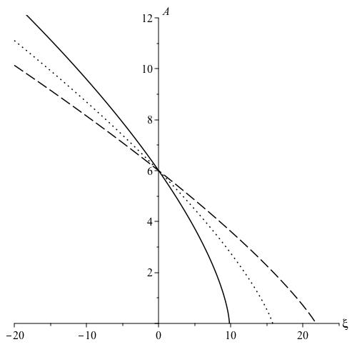
Figure 1. $C=0$: area profile for $\gamma/\mu=$ $0$ (solid), $1$ (dot), $2$ (dash).

Extending $A(\xi)$ to be a piecewise solution that is $0$ past $\xi=\xi_{0}$, then this describes a blood vessel that is filling behind the front $x=\xi_{0}+ct$ of a moving blood flow pulse and that is constricted ahead of the front, with the blood flow velocity being the same as the speed of the front, $\bar{u}=c$.

5.2. Solutions for $C<0$

In this case, equation (61) has the quadrature

$$2\mu|C|^{3/2}\arctan\big{(}\sqrt{A}/\sqrt{|C|}\big{)}-(\sigma/|C|)\ln(A)-(\gamma|C|-\sigma/|C|)\ln(A+|C|)$$ (63)

$$+\tfrac{2}{3}\mu A^{3/2}+\gamma A-2\mu|C|\sqrt{A}=\kappa(\xi_{0}-\xi)$$

which determines $A(\xi)$. By translation symmetry, it is convenient to put $\xi_{0}=0$, which corresponds to a shift in either the $x$ or $t$ coordinates. Solutions exhibit the following two different behaviours, which are distinguished by whether $A(\xi)\gtrless A_{\text{c}}$.

If $A(\xi)>A_{\text{c}}$, then the solution $A(\xi)$ is a concave decreasing function of $\xi$ that exhibits an inverted one-sided cusp at $\xi=\xi_{\text{c}}$, and the solution does not exist for $\xi>\xi_{\text{c}}$. From equation (52), $Q(\xi)=c(A(\xi)+|C|)$ has a similar behaviour, except for a constant offset. Thus, $\bar{u}(\xi)=c(1+|C|/A(\xi))$ is a positive, convex increasing function of $\xi$, with a one-sided cusp at $\xi=\xi_{\text{c}}$. See Fig. 2.

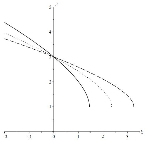
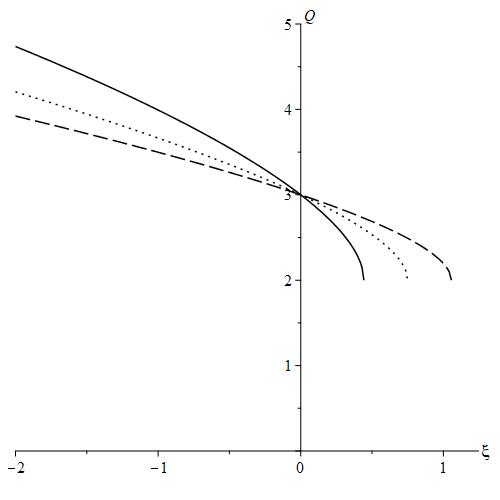
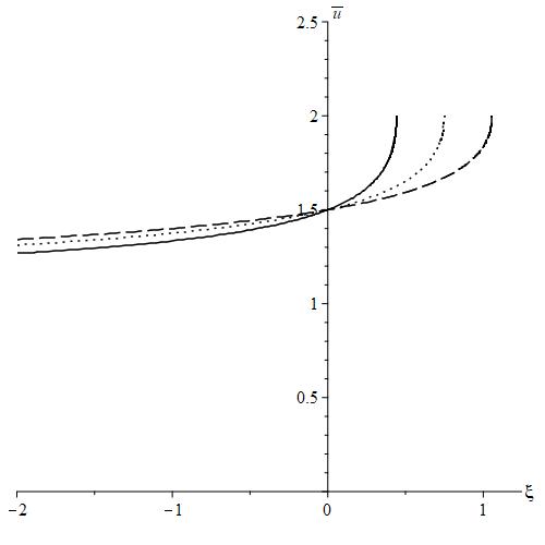
Figure 2. $C<0$, $A(\xi)>A_{\text{c}}$: area, blood flow, blood velocity profiles for $\gamma/\mu=$ $0$ (solid), $1$ (dot), $2$ (dash).

By extending $(A(\xi),Q(\xi),\bar{u}(\xi))$ as a piecewise (continuous) solution that is constant past $\xi=\xi_{\text{c}}$, this describes a blood vessel that is expanding behind the sharp front $x=\xi_{\text{c}}+ct$ of a moving blood flow pulse. The blood velocity exceeds the speed $c$ of the pulse ahead of the front, and dips down to the pulse speed $c$ far behind the front, such that the rate of change spikes at the front, $\bar{u}_{x}|_{x=\xi_{\text{c}}+ct}=\infty$.

If $A(\xi)<A_{\text{c}}$, then the solution behaviour is that $A(\xi)$ goes to zero exponentially as $\xi\to-\infty$ and is a convex increasing function of $\xi$ with a one-sided cusp at $\xi=\xi_{\text{c}}$. $Q(\xi)=c(A(\xi)+|C|)$ again has a similar behaviour with a constant offset, and $\bar{u}(\xi)=c(1+|C|/A(\xi))$ is a decreasing positive function of $\xi$ with an inverted at $\xi=\xi_{\text{c}}$ where $\bar{u}(\xi_{\text{c}})=c(1+|C|/A_{\text{c}})>0$. See Fig. 3.

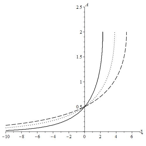
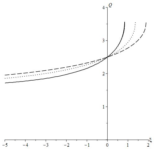
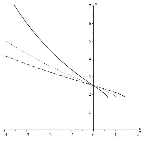
Figure 3. $C<0$, $A(\xi)<A_{\text{c}}$: area, blood flow, blood velocity profiles for $\gamma/\mu=$ $0$ (solid), $1$ (dot), $2$ (dash).

Extension of $(A(\xi),Q(\xi),\bar{u}(\xi))$ as a piecewise (continuous) solution that is constant past $\xi=\xi_{\text{c}}$ describes a blood vessel that is constricting behind the sharp front $x=\xi_{\text{c}}+ct$ of a moving blood flow pulse. The blood velocity $\bar{u}$ exceeds the speed $c$ of the pulse ahead of the front, and rises behind the front, such that the rate of change spikes at the front, $\bar{u}_{x}|_{x=\xi_{\text{c}}+ct}=-\infty$.

5.3. Solutions for $C>0$

In this case, the quadrature of equation (61) for $A(\xi)$ is given by

$$\mu C^{3/2}\ln\big{(}|\sqrt{C}-\sqrt{A}|/(\sqrt{C}+\sqrt{A})\big{)}+(\sigma/C)\ln(A)+(\gamma C-\sigma/C)\ln(|C-A|)$$ (64)

$$+\tfrac{2}{3}\mu A^{3/2}+\gamma A+2\mu C\sqrt{A}=\kappa(\xi_{0}-\xi).$$

Again, it is convenient to put $\xi_{0}=0$ by translation symmetry. Solutions exhibit several different behaviours, which are distinguished by whether $A(\xi)\gtrless A_{\text{c}}$ and $A(\xi)\gtrless C$ and also whether $A_{\text{c}}\gtrless C$, as follows.

The solutions in the case $A_{\text{c}}>C$ will be discussed first.

Suppose $A(\xi)>A_{\text{c}}>C$. The qualitative solution behaviour is similar to the corresponding case when $C<0$: $A(\xi)$ and $Q(\xi)=c(A(\xi)-C)$ are positive concave decreasing functions of $\xi$, which have an inverted one-sided cusp at $\xi=\xi_{\text{c}}$ where the solution stops. Thus, $\bar{u}(\xi)=c(1-C/A(\xi))$ is a positive convex increasing function that exponentially approaches the value $0$ as $\xi\to-\infty$ and has a one-sided cusp at $\xi=\xi_{\text{c}}$. See Fig. 4.

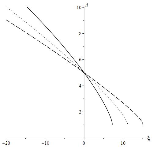
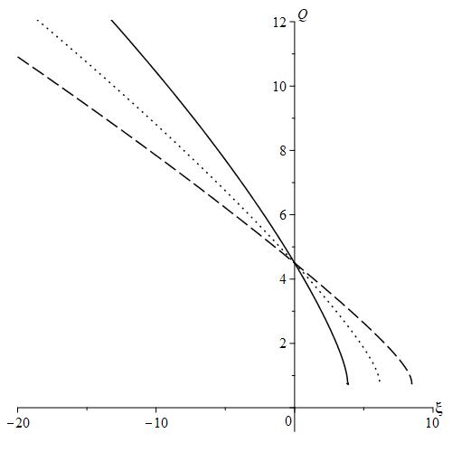
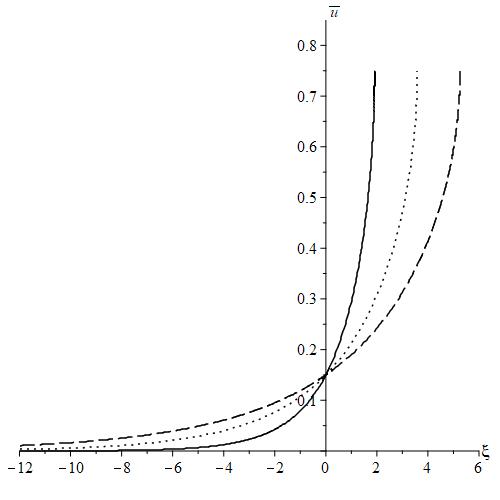
Figure 4. $A(\xi)>A_{\text{c}}>C>0$: area, blood flow, blood velocity profiles for $\gamma/\mu=$ $0$ (solid), $1$ (dot), $2$ (dash).

By extending $(A(\xi),Q(\xi),\bar{u}(\xi))$ as a piecewise (continuous) solution that is constant past $\xi=\xi_{\text{c}}$, this describes a blood vessel that is expanding behind the sharp front $x=\xi_{\text{c}}+ct$ of a moving blood flow pulse. The blood velocity $\bar{u}$ is less than the speed $c$ of the pulse ahead of the front, and drops to zero behind the front, such that there is a spike in the rate of change at the front, $\bar{u}_{x}|_{x=\xi_{\text{c}}+ct}=\infty$.

Suppose $A_{\text{c}}>A(\xi)>C$. The qualitative solution behaviour is again similar to the corresponding case when $C<0$: $A(\xi)$, $Q(\xi)=c(A(\xi)-C)$, and $\bar{u}(\xi)=c(1-C/A(\xi))$ are positive increasing functions which exhibit a one-sided cusp at $\xi=\xi_{\text{c}}$, and the solution does not exist for $\xi>\xi_{\text{c}}$. As $\xi\to-\infty$, $A(\xi)$ approaches the value $C>0$ exponentially, while $Q(\xi)$ and $\bar{u}(\xi)$ go to zero. See Fig. 5.

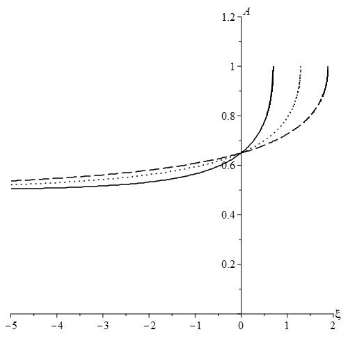
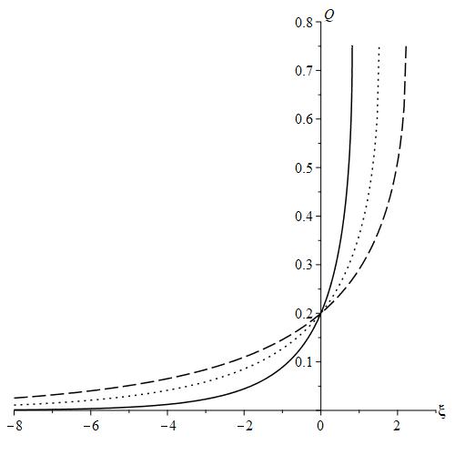
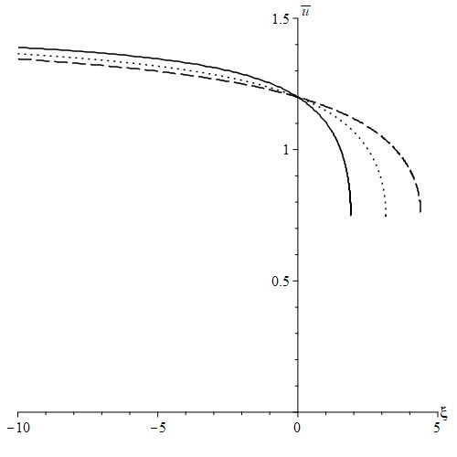
Figure 5. $A_{\text{c}}>A(\xi)>C>0$: area, blood flow, blood velocity profiles for $\gamma/\mu=$ $0$ (solid), $1$ (dot), $2$ (dash).

Extension of $(A(\xi),Q(\xi),\bar{u}(\xi))$ as a piecewise (continuous) solution that is constant past $\xi=\xi_{\text{c}}$ describes a blood vessel that contracts sharply inward to a constant diameter behind the front $x=\xi_{\text{c}}+ct$ of a moving blood pulse at which the rate of decrease in area and blood flow have a spike. The blood velocity $\bar{u}$ is less than the speed $c$ of the pulse ahead of the front, and rises slowly to the speed of the pulse behind the front, such that there is a spike in the rate of change at the front, $\bar{u}_{x}|_{x=\xi_{\text{c}}+ct}=-\infty$.

For $A_{\text{c}}>C>A(\xi)$, a different behaviour arises. The solution exists for all $\xi$ and has the asymptotic behaviour that $A(\xi)$ decreases exponentially to $0$ as $\xi\to\infty$, and exponentially approaches the value $C$ as $\xi\to-\infty$. Consequently, $Q(\xi)=c(A(\xi)-C)$ is a negative function that exponentially approaches the value $0$ as $\xi\to-\infty$ and decreases to the value $-cC$ as $\xi\to\infty$. Therefore, $\bar{u}(\xi)=c(1-C/A(\xi))$ is a negative decreasing function that exponentially approaches the value $0$ as $\xi\to-\infty$ but has no lower bound as $\xi\to\infty$. See Fig. 6.

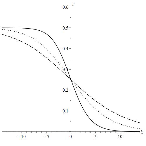
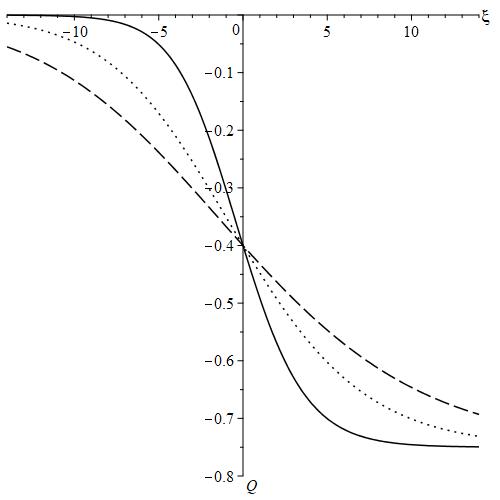
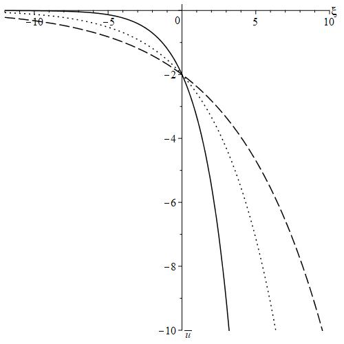
Figure 6. $A_{\text{c}}>C>A(\xi)>0$: area, blood flow, blood velocity profiles for $\gamma/\mu=$ $0$ (solid), $1$ (dot), $2$ (dash).

This describes a blood vessel in which there is a moving compressive pulse with a shock front that causes the blood flow to be in the backward direction. Far ahead of the pulse, the blood vessel is constricted such that the diameter is close to zero, while at the front of the pulse, where convexity of the cross-section area vanishes, the blood flow exhibits a sharp transition from a high flow value to a low flow value.

Next, the solutions in the case $C>A_{\text{c}}$ will be discussed.

Suppose $A(\xi)>C$. The solution $A(\xi)$ is a positive concave decreasing function of $\xi$ that exponentially approaches the value $C$ as $\xi\to\infty$, while $Q(\xi)=c(A(\xi)-C)$ has a similar behaviour but goes to $0$ as $\xi\to\infty$. Thus, $\bar{u}(\xi)=c(1-C/A(\xi))$ is a positive decreasing function that exponentially goes to $0$ as $\xi\to\infty$. See Fig. 7.

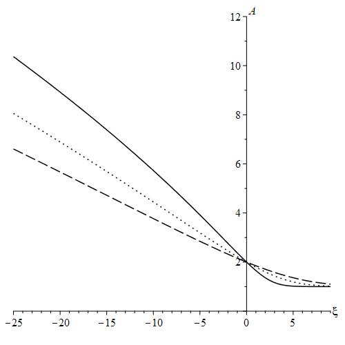
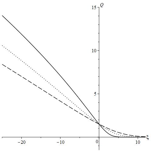
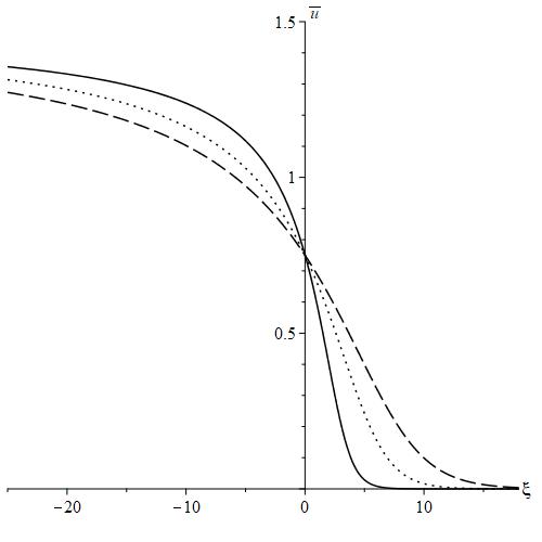
Figure 7. $A(\xi)>C>A_{\text{c}}>0$: area, blood flow, blood velocity profiles for $\gamma/\mu=$ $0$ (solid), $1$ (dot), $2$ (dash).

This describes a blood vessel whose diameter increases as the blood flows forward along the vessel. Unlike previous cases, the pulse does not have a sharp front, but there is a transition point where the rate of decrease in blood flow and velocity reaches a maximum, with the velocity tapering to zero ahead of this point. The blood velocity resembles a shock whose front, where the convexity vanishes, corresponds to the transition point.

Suppose $C>A(\xi)>A_{\text{c}}$. The solution $A(\xi)$ is a positive concave increasing function of $\xi$ that starts as an inverted one-sided cusp at $\xi=\xi_{\text{c}}$ and exponentially approaches the value $C$ as $\xi\to\infty$. Likewise, $Q(\xi)=c(A(\xi)-C)$ and $\bar{u}(\xi)=c(1-C/A(\xi))$ start with an inverted negative one-sided cusp at $\xi=\xi_{\text{c}}$ and are increasing functions of $\xi$ that exponentially approach $0$ as $\xi\to\infty$. See Fig. 8.

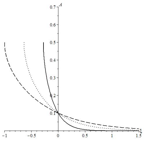
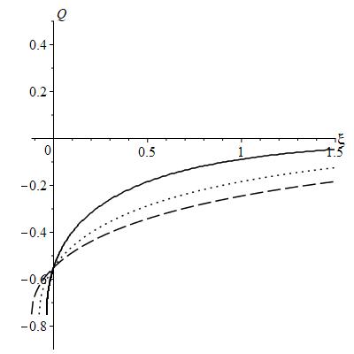
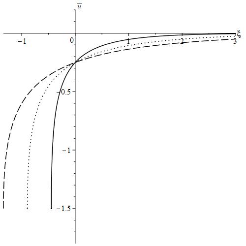
Figure 8. $C>A(\xi)>A_{\text{c}}>0$: area, blood flow, blood velocity profiles for $\gamma/\mu=$ $0$ (solid), $1$ (dot), $2$ (dash).

Extending $(A(\xi),Q(\xi),\bar{u}(\xi))$ as a piecewise (continuous) solution that is constant prior to $\xi=\xi_{\text{c}}$, then this describes a blood vessel in which there is a backward pulse of blood flow with a sharp front $x=\xi_{\text{c}}+ct$ that moves forward at speed $c$. Ahead of the front, the vessel is constricted and the blood velocity $\bar{u}$ is close to zero, while at the front the diameter flares to a constant size $2\sqrt{A_{1}/\pi}$ and the backward velocity rapidly rises up to the speed $c$ of the pulse at the front.

A different behaviour occurs for $A_{\text{c}}>A(\xi)$. The solution $A(\xi)$ is a positive convex decreasing function of $\xi$ that starts as a one-sided cusp at $\xi=\xi_{\text{c}}$ and exponentially approaches $0$ as $\xi\to\infty$. $Q(\xi)=c(A(\xi)-C)$ starts as a negative one-sided cusp at $\xi=\xi_{\text{c}}$ and decreases with $\xi$ such that it exponentially goes to $0$ as $\xi\to\infty$. $\bar{u}(\xi)=c(1-C/A(\xi))$ similarly is a negative decreasing function of $\xi$ that starts with a one-sided cusp at $\xi=\xi_{\text{c}}$, but it has no lower bound as $\xi\to\infty$. See Fig. 9.

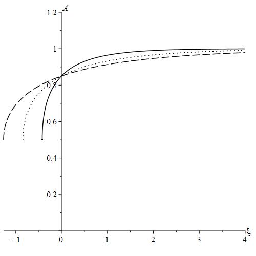
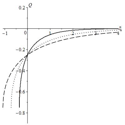
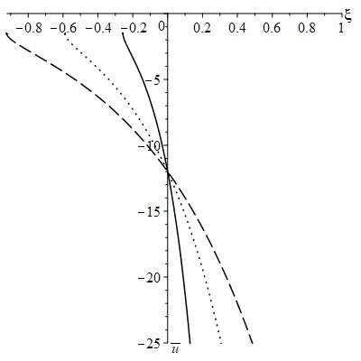
Figure 9. $C>A_{\text{c}}>A(\xi)>0$: area, blood flow, blood velocity profiles for $\gamma/\mu=$ $0$ (solid), $1$ (dot), $2$ (dash).

Extension of $(A(\xi),Q(\xi),\bar{u}(\xi))$ as a piecewise (continuous) solution that is constant prior to $\xi=\xi_{\text{c}}$ describes a blood vessel that rapidly collapses to a constant diameter $2\sqrt{A_{1}/\pi}$ behind the sharp front $x=\xi_{\text{c}}+ct$ of moving pulse with speed $c$. The blood flow and velocity are in the backward direction and their rate of change spikes at the front, $Q_{x}|_{x=\xi_{\text{c}}+ct}=-\infty$ and $\bar{u}_{x}|_{x=\xi_{\text{c}}+ct}=\infty$. Ahead of the front, the blood flow tapers to zero while the blood velocity is rising in magnitude.

Last, consider the case $A_{\text{c}}=C>0$. The root equation (56) yields $A_{c}=A_{*}$ where

$$A_{*}=(\tfrac{2\rho_{0}c^{2}}{\mu})^{2},$$ (65)

and equation (61) for $A(\xi)$ becomes

$$A^{\prime}=\frac{\kappa A}{(A+C)(\gamma+\mu A^{3/2})}.$$ (66)

Its quadrature is given by

$$\gamma A_{*}\ln(A)+\tfrac{2}{3}\mu A^{3/2}+\gamma A+2\mu A_{*}\sqrt{A}=\kappa(\xi_{0}-\xi).$$ (67)

The solution behaviour in this case is similar to the earlier case $A(\xi)>A_{\text{c}}>C$, except that here $A(\xi)$ goes to $0$ exponentially, $Q(\xi)=c(A(\xi)-A_{*})$ changes sign and goes to $-cA_{*}$ exponentially, while $\bar{u}(\xi)=c(1-A_{*}/A(\xi))$ changes sign and decreases with no lower bound.

A useful final remark is that

$$\mathrm{sgn}(A_{\text{c}}-C)=\mathrm{sgn}(A_{*}-C)$$ (68)

can be shown to hold from the root equation (56) by the following argument. First, use the relations (51) to write equation (56) as $\tilde{\gamma}A_{\text{c}}^{2}+\tilde{\mu}A_{\text{c}}^{5/2}=C^{2}$ where $\tilde{\gamma}=1-\tfrac{1}{\alpha}\geq 0$ and $\tilde{\mu}=\tfrac{\mu}{2\alpha c^{2}}>0$ which do not involve $C$. Then, for $A_{\text{c}}=C\neq 0$, $C=(\tfrac{1-\tilde{\gamma}}{\tilde{\mu}})^{2}=A_{*}$. Next, view $A_{\text{c}}-C:=f(C)$ as a function of $C$. The root equation shows that the solutions of $f(C)=0$ are $C=A_{*}$ and $C=0$, and that $f^{\prime}(A_{*})=-\tfrac{1-\tilde{\gamma}}{5-\tilde{\gamma}}=-\tfrac{1}{4\alpha+1}$ is negative. This implies $f(C)>0$ for $0<C<A_{*}$ and $f(C)<0$ for $C>A_{*}$, which establishes the sign relation (68).

6. Concluding remarks

In the present work, symmetry analysis has been applied to a widely used 1D model of blood flow in a single blood vessel, with a general pressure-area relation. Several new results have been obtained.

One main result is that three new conservation laws have been derived in case of inviscid flow. These conservation laws yield conserved integrals describing generalized momentum and generalized volumetric and axial energies. The generalized momentum differs compared to the momentum in inviscid constant-density 1D fluid dynamics by involving powers of $A$ that depend on $\alpha-1$, where $\alpha$ is the momentum correction coefficient. Likewise, when $\alpha\neq 1$, both of the generalized energies involve different powers of $A$ compared to the energy in inviscid constant-density fluid dynamics. In the case of viscous blood flow, each conservation law gets replaced by a balance equation containing a dissipative volume term proportional to the friction coefficient in the model.

These conservation laws can be expected to be useful in analysis of the model [4]. In particular, they can provide conserved norms and enable the derivation of time-decay inequalities; they can also be used for checking the accuracy of numerical schemes.

Another main result is that travelling wave solutions have been studied in detail. Prior to this contribution, the only exact solutions which have been studied in the literature were steady-state solutions. Firstly, general features of the travelling wave solutions have been discussed and shown to be qualitatively independent of the specific form of the pressure-area relation in the model. Secondly, all travelling waves have been derived explicitly for the simplest and most commonly considered case where the pressure change across the blood vessel wall is proportional to the change in radius. These solutions are most naturally applicable to the idealized case of a very long blood vessel in which the morphology of ends is not relevant, as the spatial domain of a solution in this situation is unbounded. For a blood vessel whose morphology at the ends is important for understanding the blood flow behaviour, travelling wave solutions are still applicable by considering suitable boundary conditions. Specifically, while travelling waves do not describe common morphologies such as a fixed diameter or pressure, or a fixed blood flow, in a blood vessel, nevertheless they may be relevant if conditions in the vessel wall or surrounding tissue cause a persistent wave pulse to propagate axially with constant speed. They may also be relevant in constructing piecewise solutions for approximating more realistic wave forms [29]. Travelling waves also include steady-state (time-independent) solutions as a special case when the wave speed is zero, and these solutions are compatible with all standard morphological boundary conditions.

A variety of interesting behaviours exhibited by the travelling waves have been found, including:
$\bullet$ pressure shocks;
$\bullet$ blood flow shocks;
$\bullet$ sharp wave-front pulses in pressure and blood flow;
$\bullet$ flows in which the blood vessel is expanding or constricting.

All of the new results show the utility of symmetry analysis for providing explicit analytical information about exact non-steady solutions and conservation laws.

There are several possible directions for future work: (1) understand piecewise solutions in a framework of weak solutions; (2) examine stability of the solutions; (3) derive and apply energy inequalities in the study of the initial-value problem; (4) study similarity solutions using scaling and dilation symmetries; (5) consider improved models, for example, by inclusion of a diffusion term, use of a viscoelastic tube law, and an improved radial velocity profile.

References

- [1] E. Marchandise, M. Willemet, V. Lacroix, A numerical hemodynamic tool for predictive vascular surgery, Med. Eng. Phys. 31 (2009), 131–144.
- [2] C. Audebert, P. Bucur, M. Bekheit, E. Vibert, I.E. Vignon-Clementel, J. Gerbeau, Kinetic scheme for arterial and venous blood flow, and application to partial hepatectomy modeling, Comput. Methods Appl. Mech. Eng. 314 (2017), 102–125.
- [3] S. Sherwin, L. Formaggia, J. Peiro, V. Franke, Computational modelling of 1D blood flow with variable mechanical properties and its application to the simulation of wave propagation in the human arterial system, Int. J. Numer. Methods Fluids 43(6-7) (2003), 673–700.
- [4] L. Formaggia, D. Lamponi, A. Quarteroni, One-dimensional models for blood flow in arteries, J. Engineering Math. 47 (2003), 251–276.
- [5] L. Formaggia, A. Moura, F. Nobile, On the stability of the coupling of 3D and 1D fluid-structure interaction models for blood flow simulations, ESAIM: M2AN 41(4) (2007), 743–769.
- [6] N. Xiao, J. Alastruey, C.A. Figueroa, A systematic comparison between 1-D and 3-D hemodynamics in compliant arterial models, Int. J. Numer. Method. Biomed. Eng. 30(2) (2013), 204–231.
- [7] T. Dobroserdova, F. Liang, G. Panasenko, Y. Vassilevski, Multiscale models of blood flow in the compliant aortic bifurcation, Appl. Math. Lett. 93 (2019), 98–104.
- [8] A.C. Barnard, W.A. Hunt, W.P. Timlake, E. Varley, A theory of fluid flow in compliant tubes, Biophys. J. 6(6) (1966), 717–724.
- [9] S.I. Mukhin, M.A. Menyailova, N.V. Sosnin, A.P. Favorskii, Analytic Study of Stationary Hemodynamic Flows in an Elastic Vessel with Friction, Diff. Equat. 43 (2007), 1011–1015.
- [10] B. Ghitti, C. Berthon, M. Hoang Le, E.F. Toro, A fully well-balanced scheme for the 1D blood flow equation with friction source term, J. Comput. Phys. 421 (2020), 109750.
- [11] J. Britton, Y. Xing, Well-balanced discontinuous Galerkin methods for the one-dimensional blood flow through arteries model with man-at-eternal-rest and living-man equilibria, Comput. Fluids 203 (2020), 104493.
- [12] C. Spiller, E.F. Toro, M.E. Vázquez-Cendón, C. Contarino, On the exact solution of the Riemann problem for blood flow in human veins, including collapse, Appl. Math. Comput. 303 (2017), 178–189.
- [13] W. Sheng, Q. Zhang, Y. Zheng, The Riemann problem for a blood flow model in arteries, Commun. Comput. Phys. 27(1) (2020), 227–250.
- [14] Y.V Vassilevski, V.Y. Salamatova, S.S. Simakov, On the elasticity of blood vessels in one-dimensional problems of hemodynamics, Comput. Math. Math. Phys. 55(9) (2015), 1567–1578.
- [15] I. Sazonov, P. Nithiarasu, A novel, FFT‑based one‑dimensional blood fow solution method for arterial network, Biomech. Model. Mechanobiol. 18 (2019), 1311–1334.
- [16] A. Quarteroni, L. Formaggia, Mathematical modelling and numerical simulation of the cardiovascular system. In: Computational Models for the Human Body (ed. N. Ayache), Handbook of Numerical Analysis Vol. 12, 2004, 3–127.
- [17] G. V. Krivovichev, Comparison of inviscid and viscid one-dimensional models of blood flow in arteries, Appl. Math. Comput. 418 (2022), 126856.
- [18] L.V. Ovsiannikov, Group Analysis of Differential Equations, Academic Press: New York, 1982.
- [19] N.H. Ibragimov (ed.) Lie Group Analysis of Differential Equations, Vol 1, Symmetries, Exact Solutions and Conservation Laws, CRC: Boca Raton, 2009.
- [20] R. Jiwari, V. Kumar, S. Singh, Lie group analysis, exact solutions and conservation laws to compressible isentropic Navier-Stokes equation, Eng. Comput. 38 (2022), 2027–2036.
- [21] P.J. Olver, Applications of Lie Groups to Differential Equations, Springer-Verlag: New York, 1993.
- [22] G.W. Bluman, A. Cheviakov, S.C. Anco, Applications of Symmetry Methods to Partial Differential Equations, Springer: New York, 2009.
- [23] G.M. Webb, G.P. Zank, Scaling symmetries, conservation laws and action principles in one-dimensional gas dynamics, J. Phys. A: Math. Theor. 42 (2009), 475205.
- [24] G.K. Batchelor, An introduction to fluid dynamics, Cambridge University Press, 2000.
- [25] S.C. Anco, G.W. Bluman, Direct construction method for conservation laws of partial differential equations Part II: General treatment, Euro. J. Appl. Math. 41 (2002), 567–585.
- [26] S.C. Anco, Generalization of Noether’s theorem in modern form to non-variational partial differential equations. In: Recent progress and Modern Challenges in Applied Mathematics, Modeling and Computational Science (eds. R. Melnik et al), 119–182. Fields Institute Communications, Volume 79, 2017.
- [27] L. Grinberg, G.E. Karniadakis, Outflow boundary conditions for arterial networks with multiple outlets, Ann. Biomed. Eng. 36 (2008), 1496–1514.
- [28] J. Alastruey, K.H. Parker, S.J. Sherwin, Arterial pulse wave haemodynamics. In: 11th International Conference on Pressure Surges (ed. S. Anderson), 401–443. Virtual PiE Led t/a BHR Group, 2012.
- [29] M. Anliker, W.E. Moritz, E. Ogden, Transmission characteristics of axial waves in blood vessels, J. Biomech. 1 (1968), 235–246.