Analog black-white hole solitons in traveling wave parametric amplifiers with superconducting nonlinear asymmetric inductive elements

Abstract

We show that existing travelling wave parametric amplifier (TWPA) setups, using superconducting nonlinear asymmetric inductive elements (SNAILs), admit soliton solutions that act as analogue event horizons. The SNAIL-TWPA circuit dynamics are described by the Korteweg-de Vries (KdV) or modified Korteweg-de Vries (mKdV) equations in the continuum field approximation, depending on the external magnetic flux bias, and validated numerically. The soliton spatially modulates the velocity for weak probes, resulting in the effective realization of analogue black hole and white hole event horizon pairs. The SNAIL external magnetic flux bias tunability facilitates a three-wave mixing process, which enhances the prospects for observing Hawking photon radiation.

Introduction.— Analogue black holes have been proposed in various laboratory systems as a means of verifying the basic principle of Hawking radiation [1], which could provide a clue for unifying gravity and quantum mechanics. In 1981, Unruh pioneered the study of analogue black holes by showing the analogy between the behavior of sound waves in a transsonic fluid flow and that of light in the spacetime of a black hole [2]. The basic idea is to create a spatially varying fluid flow so that sound waves cannot escape from a certain boundary corresponding to a black hole event horizon (i.e., a sonic event horizon). Based on this idea, thermal properties of stimulated Hawking emission and the correlations that are associated with the Hawking effect have been observed in a water flume [3, 4]. But such experiments cannot capture the quantum spontaneous emission aspects of Hawking radiation due to the overwhelming classical thermal noise.

In order to observe quantum effects, analogue black holes have been proposed in various systems such as Bose-Einstein condensates [5, 6], optical fibers [7, 8, 9], and superfluids in polariton microcavities [10, 11]. Cryogenic, superconducting transmission line circuits have advantages over the above schemes in controllability, scalability, and low noise operation, making the detection of quantum correlated Hawking radiation involving photons a very real possibility [12, 13, 14]. A spatially varying microwave velocity is a necessary requirement for creating an analogue black hole in such a circuit [15, 16, 17, 18, 19, 20, 21]. This can be achieved by introducing an effective spatially dependent inductance $L$ or capacitance $C$, since the electromagnetic wave velocity is given by $v=a/\sqrt{LC}$ with unit cell length $a$. The problem of heating that hinders the observation of Hawking radiation [15] has been addressed by using superconducting circuits [16]. Additionally, the issue of pulse instability arising from dispersion has been overcome by utilizing solitons [17], leading to classically stable horizons. However, there is still some way to go in terms of realizing the design, fabrication and measurements in order to successfully observe Hawking radiation. One unexpected obstacle is the Kerr effect itself inherent in conventional Josephson systems, i.e., the fourth-order nonlinearity of the Josephson effect required for soliton formation as well as the Hawking pair creation from the vacuum. The Kerr interaction causes higher-order harmonic generation due to four-wave mixing, which reduces the degree of entanglement and squeezing performance essential for Hawking radiation detection [22, 23].

A three-wave mixing process caused by a third-order nonlinear potential can improve these aspects. However, the ordinary Josephson effect alone cannot produce odd-order nonlinearities such as a cubic potential. One way to achieve this is through a superconducting nonlinear asymmetric inductive element (SNAIL) [24], which is a superconducting loop consisting of a single small Josephson junction (JJ) and several larger junctions in parallel as shown in Fig. 1. This results in a third-order nonlinear effect, in addition to the leading fourth-order nonlinear effect of a single JJ. Travelling wave parametric amplifier (TWPA) transmission line devices incorporating SNAILs have demonstrated remarkable results in recent experiments [25, 26]. Specifically, parametrically-generated multimode entangled microwave photons were successfully observed, which highlights the promising prospect for generating and detecting Hawking radiation in such devices. However, it is not a priori obvious whether such a third-order nonlinearity can give rise to a soliton with an analogue black hole event horizon.

In this letter, we propose an analogue black hole soliton realization based on a Kerr-free nonlinearity using a transmission line comprising SNAIL unit cells. In particular, we shall establish both analytically and numerically the existence of soliton solutions to the nonlinear transmission line dynamical equations for the SNAIL phase difference coordinates. These obtained solitons spatially modulate the velocity of weak ‘probes’ and two stable horizons occur where the probe and soliton velocities coincide, resulting in an analogue black hole and white hole horizon pair. Neglecting (quantum) noise and dissipation in the circuit dynamics, a soliton will propagate along the transmission line without broadening, in contrast to a background ‘pulse’ solution to the linear phase coordinate wave equations, which undergoes dispersion [16]. This stability has the advantage that the effective Hawking temperature (which depends on the probe velocity gradient at the effective horizon) does not decrease as the soliton propagates (with backreaction neglected).

Model.—Consider a transmission line with SNAILs as shown in Fig. 1, where the Josephson energy of the small and large junctions are $\alpha E_{J}$ and $E_{J}$, respectively (with $\alpha<1$), and all capacitors have the identical capacitance $C_{g}$ in the shunt branch. In the following, we consider the circuit equations of the transmission line, beginning first with the potential energy of a single SNAIL, which is given as

$$U\left(\phi\right) =-\alpha E_{J}\cos\left(\phi\right)-2E_{J}\cos\left(\frac{\phi-\phi_{{\mathrm{ext}}}}{2}\right)+{\mathrm{const.}},$$

$$\simeq\!E_{J}\left[\!\frac{\tilde{\alpha}(\phi_{{\mathrm{ext}}})}{2!}{\tilde{\phi}}^{2}+\frac{\tilde{\beta}(\phi_{{\mathrm{ext}}})}{3!}{\tilde{\phi}}^{3}+\frac{\tilde{\gamma}(\phi_{{\mathrm{ext}}})}{4!}{{\tilde{\phi}}}^{4}\!\right].$$ (1)

Here, $\phi$ is the phase difference across the smaller junction and $\phi_{{\mathrm{ext}}}=2\pi\Phi_{{\mathrm{ext}}}/\Phi_{0}$, with $\Phi_{{\mathrm{ext}}}$ and $\Phi_{0}=h/(2e)$ the (tunable) external magnetic flux bias and magnetic flux quantum, respectively, and the Taylor expansion around the local minimum $\phi^{\ast}$ of the potential is performed, with $\tilde{\phi}$ being the variation about $\phi^{\ast}$ and setting $U\left(\phi^{\ast}\right)=dU/d\phi|_{\phi=\phi^{\ast}}=0$. In contrast to a single JJ, the SNAIL has the advantage of a non-zero, odd-order nonlinearity because of quantum interference. Figure 2 gives the $\phi_{{\mathrm{ext}}}$ flux dependence of these coefficients normalized by $\tilde{\alpha}\left(\phi_{{\mathrm{ext}}}\right)$ [i.e., $c_{3}=\tilde{\beta}\left(\phi_{{\mathrm{ext}}}\right)/\tilde{\alpha}\left(\phi_{{\mathrm{ext}}}\right)$, $c_{4}=\tilde{\gamma}\left(\phi_{{\mathrm{ext}}}\right)/\tilde{\alpha}\left(\phi_{{\mathrm{ext}}}\right)$]. The coefficients of the third and fourth-order nonlinearities are anticorrelated, and either can be selectively set to zero by tuning $\phi_{\mathrm{ext}}$. Thus, we can choose either a three or four-wave mixing process induced by the third or fourth-order nonlinearities, respectively, by controlling the external magnetic flux in situ, without the need to alter the circuit design hardware.

Figure 1: Schematic diagram of the traveling wave parametric amplifier (TWPA) transmission line with superconducting nonlinear asymmetric inductive element (SNAIL) unit cells in series, alternating with shunt capacitors $C_{g}$ in parallel (all assumed identical). The quantities $I_{n}$, $V_{n}$, and $\phi_{n}$ represent the current, voltage, and phase difference of the $n$th SNAIL, respectively. Each SNAIL has a small JJ with Josephson energy $\alpha E_{J}$ ($\alpha<1$) in one branch and two larger JJs (with Josephson energy $E_{J}$) in the other, parallel branch, forming a loop that is threaded by an external applied magnetic flux $\Phi_{{\mathrm{ext}}}$.

Figure 2: The external flux $\phi_{{\mathrm{ext}}}$ dependence of the respective third and fourth order nonlinear coefficients $c_{3}=\tilde{\beta}\left(\phi_{{\mathrm{ext}}}\right)/\tilde{\alpha}\left(\phi_{{\mathrm{ext}}}\right)$ (solid line) and $c_{4}=\tilde{\gamma}\left(\phi_{{\mathrm{ext}}}\right)/\tilde{\alpha}\left(\phi_{{\mathrm{ext}}}\right)$ (dashed line) of a SNAIL.

With the approximate potential energy of the SNAIL in hand, we can write down the circuit equations for the TWPA. From Kirchhoff’s current conservation law and the Josephson voltage relation, we obtain the following circuit equations:

$$\frac{d^{2}\phi_{n}}{dt^{2}}-r\frac{d^{2}}{dt^{2}}\left(\phi_{n+1}-2\phi_{n}+\phi_{n-1}\right)$$

$$-\omega_{0}^{2}\sum^{3}_{j=1}\left[\frac{c_{j+1}}{j!}\left(\phi^{j}_{n+1}-2\phi^{j}_{n}+\phi^{j}_{n-1}\right)\right]=0,$$ (2)

where $c_{2}=1$, $r=C_{J}/C_{g}$ with $C_{g}$ the shunt capacitance and $C_{J}$ the Josephson capacitance of the SNAIL, and $\omega_{0}=1/\sqrt{L_{0}C_{g}}$ with $L_{0}=\hbar/\left[2eI_{c}\tilde{\alpha}\left(\phi_{{\mathrm{ext}}}\right)\right]$ and $I_{c}$ the critical current of the larger JJ in the SNAIL.

In the continuum approximation, the circuit equation (2) becomes [27]

$$\frac{\partial^{2}\phi}{\partial t^{2}}\!-\!ra^{2}\frac{\partial^{4}\phi}{\partial x^{2}\partial t^{2}}\!-\!v_{0}^{2}\frac{\partial^{2}}{\partial x^{2}}\left(\phi+\frac{c_{3}}{2!}\phi^{2}+\frac{c_{4}}{3!}\phi^{3}\right)=0,$$ (3)

where $v_{0}=a\omega_{0}$ with unit cell length $a$. The second (fourth order derivative) term gives rise to dispersion, while the last two terms are the third and fourth order nonlinearities, respectively (where the order terminology refers to the degree of the nonlinearity in the potential energy function). Equation (3) is equivalent to Eq. (7) in [27] by replacing the phase difference coordinate $\phi$ with the node phase coordinate.

Classical background solitons.—With eventual, Hawking radiation signals in mind, we wish to consider the behavior of a weak ‘probe’ signal $\delta\phi$ (which when quantized yields Hawking radiation) on top of a strong classical background $\bar{\phi}$ (which yields the analogue black hole soliton). By substituting $\phi=\bar{\phi}+\delta\phi$ into the circuit equation (3), we obtain the background dynamics expression [$\mathcal{O}(\delta\phi^{0})$ term] for $\bar{\phi}$, which coincides with Eq. (3), and the equation for the weak probe signal $\delta\phi$ affected by the background [$\mathcal{O}(\delta\phi)$ term], which we consider in the next section.

We shall now derive classical background $\bar{\phi}$ wave solutions to Eq. (3) that propagate along the TWPA without changing their shape, i.e., solitons. Such a wave is obtained when the competing effects of dispersion (which broadens a wave) and nonlinearity (which sharpens a wave) are balanced. We derive a scale-invariant nonlinear evolution equation with a stationary wave solution in the vicinity of a linear approximation by using the reductive perturbation method [28, 29, 30], which employs the so-called ‘stretched’ variables through the Gardner-Morikawa transformation: $\xi=\varepsilon^{1/2}\left(x-v_{0}t\right)$ and $\tau=\varepsilon^{3/2}t$; these correspond to slowly changing variables in relation to changes in $x$ and $t$, with $\varepsilon$ assumed small. The phase difference coordinate is expanded as follows: ${\bar{\phi}}=\varepsilon^{i}{{\bar{\phi}}}^{\left(1\right)}+\varepsilon^{2i}{{\bar{\phi}}}^{\left(2\right)}+\cdots$, where $i$ is a rational number to be determined by requiring that the dispersion and nonlinear effects are balanced.

Recall that the coefficients $c_{3}$ and $c_{4}$ of the nonlinear terms are controllable by varying the external magnetic flux $\phi_{{\mathrm{ext}}}$ (see Fig. 2); from now on, we consider the situation where either one or the other of these coefficients vanishes. For the case $c_{3}\neq 0$ and $c_{4}=0$, we obtain

$$\frac{\partial{{\bar{\phi}}}^{(1)}}{\partial\tau}+\frac{c_{3}v_{0}}{2}{{\bar{\phi}}}^{(1)}\frac{\partial{{\bar{\phi}}}^{(1)}}{\partial\xi}+\frac{r}{2}a^{2}v_{0}\frac{\partial^{3}{{\bar{\phi}}}^{(1)}}{\partial\xi^{3}}=0$$ (4)

for the balanced lowest order $\varepsilon^{3}$ dispersion and nonlinear terms, obtained by setting $i=1$. This equation is called the Korteweg-de Vries (KdV) equation [31] and is known to have soliton solutions [32]. The KdV equation can be solved by means of the inverse scattering transform method [33]. A single soliton solution is given as [33]

$${\bar{\phi}}_{\mathrm{KdV}}(x,t)=A\operatorname{sech}^{2}\left[\frac{1}{a}\sqrt{\frac{c_{3}A}{12r}}\left(x-v_{s}t\right)\right],$$ (5)

with the soliton amplitude $A$, velocity $v_{s}{=v_{0}(1+c_{3}A/6)}$, and half-width $w\sim 2a\sqrt{12r/\left(c_{3}A\right)}$. The sign of the nonlinear term $c_{3}$ changes the polarity of the soliton; when $c_{3}>0$ ($c_{3}<0$), the soliton amplitude becomes $A>0$ ($A<0$).

For the case $c_{3}{=0}$ and $c_{4}{\neq}0$, we obtain the so-called, ‘modified Korteweg-de Vries’ (mKdV) equation [34]:

$$\frac{\partial{{\bar{\phi}}}^{(1)}}{\partial\tau}+\frac{c_{4}v_{0}}{4}\left({{\bar{\phi}}}^{(1)}\right)^{2}\frac{\partial{{\bar{\phi}}}^{(1)}}{\partial\xi}+\frac{r}{2}a^{2}v_{0}\frac{\partial^{3}{{\bar{\phi}}}^{(1)}}{\partial\xi^{3}}=0$$ (6)

for the balanced lowest order $\varepsilon^{5/2}$ dispersion and nonlinear terms, obtained by setting $i=1/2$. The sign of the nonlinear ($c_{4}$) term in the mKdV equation makes a difference to the soliton solution, in contrast to the KdV equation; when $c_{4}>0$, the equation is termed ‘mKdV⁺’ and admits a bell-shaped soliton solution given by the expression ${\bar{\phi}}_{\mathrm{mKdV^{+}}}(x,t)=A\operatorname{sech}\left[(A/a)\sqrt{\left|c_{4}\right|/(12r)}\left(x-v_{s}t\right)\right]$. On the other hand, for $c_{4}<0$, the equation is termed ‘mKdV^-’ and admits a shock-wave type soliton [35, 36] given by ${\bar{\phi}}_{\mathrm{mKdV^{-}}}(x,t)=A\tanh\left[(A/a)\sqrt{|c_{4}|/(12r)}\left(x-v_{s}t\right)\right]$. Both soliton-types have amplitude $A$, velocity $v_{s}$, and half width $w\sim(2a/A)\sqrt{12r/|c_{4}|}$.

We emphasize that both types of soliton (KdV and mKdV) are predicted to exist in the very same transmission line, which has not been considered before. This prediction is based on the reductive perturbation method, and thus the SNAIL TWPA transmission line provides a unique opportunity to verify this method of analysis experimentally and understand the resulting soliton dynamics.

The above approximate, continuum field equation (m)KdV-soliton solution derivations are also verified in part by numerically solving the discrete SNAIL TWPA transmission line circuit equations (2). In particular, we consider the situation where the TWPA has a third order nonlinearity and set the parameter values to be $c_{3}=0.32$, $c_{4}=0$, and $r=0.1$. Setting the initial phase difference coordinate and phase velocity boundary values as $\phi_{n}(0)={\bar{\phi}}_{\mathrm{KdV}}(a(n-n_{0}),0)$ and $\dot{\phi}_{n}(0)=\dot{\bar{\phi}}_{\mathrm{KdV}}(a(n-n_{0}),0)$, where the dot denotes the time derivative, we confirm that the numerical solution propagates along the TWPA transmission line without changing shape and is well-approximated by the analytical solution (5) obtained by the reductive perturbation method; the numerical half-width of the soliton is about 27 unit cells when the amplitude $A=0.02$, which is large enough for the continuum approximation solution (5) to be valid.

In order to further verify the soliton aspects of the propagating wave [37], we also consider two solitons initially propagating towards each other by setting the initial phase difference coordinate and phase velocity boundary values to be $\phi_{n}(0)=\phi^{r}_{n}(0)+\phi^{l}_{n}(0)$, $\dot{\phi}_{n}(0)=\dot{\phi}^{r}_{n}(0)-\dot{\phi}^{l}_{n}(0)$, where the right (left)-propagating wave and the time derivative are given by $\phi^{r(l)}_{n}(0)={\bar{\phi}}_{\mathrm{KdV}}(a(n-n^{r(l)}_{0}),0)$ and $\dot{\phi}^{r(l)}_{n}(0)=\dot{\bar{\phi}}_{\mathrm{KdV}}(a(n-n^{r(l)}_{0}),0)$, respectively. Figure 3 shows that the later time soliton shapes are unaffected by the collision, coinciding with the earlier shapes.

We now briefly consider the observation of solitons in a possible experiment setup. The solitons may be detected by measuring the time variation in the voltage at the opposite end of the TWPA transmission line from the initial, injected pulse end. We assume various circuit parameter values comparable in magnitude to those quoted in Ref. [25]: $r=C_{J}/C_{g}=0.1$, $I_{c}=1.5\,\mu$A, $a=10\,\mu$m, $\alpha=0.2$, and $\phi_{{\mathrm{ext}}}=1.19\pi$ giving $\tilde{\alpha}(\phi_{{\mathrm{ext}}})=0.37$, $c_{3}=0.32$, and $c_{4}=0$. The voltage amplitude of the soliton with $A=0.02$ in the phase difference coordinate is estimated as $V=\frac{1}{a}\frac{\hbar}{2e}\int\frac{\partial\bar{\phi}(x^{\prime},t)}{\partial t}dx^{\prime}=\hbar\omega_{0}/(2e)\left(1+c_{3}A/6\right)A=0.86\,\mu$V and the soliton temporal width is $\Delta t=w/v_{s}=0.21$ nsec. In our SNAIL TWPA model, solitons form spontaneously when an initial pulse is injected at one end. The soliton profile can be estimated using the initial pulse via inverse scattering theory [33]. The affect of disorder in a real array will cause some attenuation of the soliton amplitude as it propagates down the transmission line [38]. The SNAIL-TWPA is engineered such as to be impedance-matched with $50~{}\Omega$ transmission lines connected at the end [25, 26] in order to minimize reflection of the soliton waves.

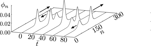
Figure 3: Collision of two solitons propagating in opposite directions. The numerical solutions of the circuit equation (2) are indicated at various time instants, where $\bar{t}=\omega_{0}t$. We set the initial right (‘$r$’) and left (‘$l$’) propagating wave values to be $A^{r}=0.04$, $A^{l}=0.02$, $n^{r}_{0}=110$, and $n^{l}_{0}=190$. The circuit parameter values are given as $c_{3}=0.32$, $c_{4}=0$, and $r=0.1$.

Soliton as analogue black and white hole event horizons.—We now move on to considering the behavior of a weak ‘probe’ (Hawking radiation) signal propagating in a background soliton field, described by the $\mathcal{O}(\delta\phi)$ part of the $\phi=\bar{\phi}+\delta\phi$ substitution into Eq. (3):

$$\left[\frac{\partial^{2}}{\partial t^{2}}-ra^{2}\frac{\partial^{4}}{\partial x^{2}\partial t^{2}}-\frac{\partial^{2}}{\partial x^{2}}v^{2}(x,t)\right]\delta\phi=0,$$ (7)

where the probe field velocity is $v\left(x,t\right)=v_{0}\sqrt{1+c_{3}{\bar{\phi}}+\frac{1}{2}c_{4}{{\bar{\phi}}}^{2}}.$ Note that the probe wave velocity is modulated by the classical background soliton solution through the space and time dependent effective inductance term $L=L_{0}/(1+c_{3}{\bar{\phi}}+\frac{1}{2}c_{4}{{\bar{\phi}}}^{2})$. Figure 4(a) gives the resulting spatial dependence of the probe velocity in the comoving frame $\eta=x-v_{s}t$ traveling at the soliton velocity $v_{s}$.

In order to derive the effective curved spacetime analogue of the probe wave (7), we first transform to the comoving frame of the soliton pulse. Equation (7) then becomes $\left[-\partial_{t}^{2}+2v_{s}\partial_{\eta}\partial_{t}+\partial_{\eta}(v^{2}(\eta)-v_{s}^{2})\partial_{\eta}\right]\delta\varphi=0,$ where the phase field coordinate $\delta\varphi$ is defined in terms of the original probe coordinate by $\delta\phi=a(d\delta\varphi/d\eta)$. This $1+1$ dimensional wave equation is conformally invariant, which prevents us from introducing an effective, curved space-time metric. However, taking into account the two additional ‘inert’ transverse $y,\,z$ dimensions of the transmission line, the resulting 3+1 dimensional wave equation can be formally expressed in the following general covariant form [15, 39]: $(1/\sqrt{-g})\partial_{\mu}\left(\sqrt{-g}g^{\mu\nu}\partial_{\nu}\delta\varphi\right)=0$, where $g=\det(g_{\mu\nu})$, and with effective metric given by

$$g^{\mu\nu}=\frac{1}{v(\eta)}\left(\begin{array}[]{cccc}-1&v_{s}&0&0\\ v_{s}&v^{2}(\eta)-v_{s}^{2}&0&0\\ 0&0&1&0\\ 0&0&0&1\\ \end{array}\right).$$ (12)

The weak probe field can therefore be considered as propagating in an effective curved space-time, and an event horizon occurs at $g_{{11}}=0$, i.e., $v^{2}(\eta)=v_{s}^{2}$. For a background field solution corresponding to a single, right-moving classical soliton traveling with velocity $v_{s}>0$, two horizons are formed as shown in Fig. 4(a), where the leading and trailing edges of the soliton correspond to the white and black hole horizons, respectively. In the comoving frame of the soliton, the probe signal travels to the right between the horizons and to the left otherwise (also in the comoving frame). A probe signal trailing the soliton (in the lab frame) cannot reach the black hole horizon, so that the region to the left of the black hole corresponds to its interior. Furthermore, a right moving probe signal in the neighborhood of the soliton peak (i.e., the ‘exterior’ region in between the black and white hole horizons) cannot cross the white hole horizon, so that the region to the right of the white hole horizon corresponds to the white hole interior.

Figure 4(b) gives the dispersion relation for a probe wave in the laboratory frame (curved solid lines) and the Doppler shift $\omega=\omega^{\prime}+v_{s}k$ (dotted straight lines), where $\omega^{\prime}$ is the fixed frequency in the comoving frame. The intersections indicate the existing modes in our system. In regions I and III, there is only one mode labelled $k_{\bar{\mathrm{H}}}$ which travels to the left in the comoving frame. On the other hand, in region II, the dispersion relation is modulated by the soliton and there exist three modes: one moving to the right ($k_{\mathrm{H}}$) and the other two travelling to the left in the comoving frame ($k_{\mathrm{P}}$ and $k_{\mathrm{N}}$, with ‘P’ and ‘N’ denoting the positive and negative frequency $\omega$ aspects). In vacuum, pair production occurs spontaneously through quantum fluctuations; photons with positive ($k_{\mathrm{H}}$) and negative ($k_{\mathrm{\bar{H}}}$) frequency $\omega$ correspond to the Hawking particles and their partners, respectively. Mode conversion ($k_{\mathrm{H}}+k_{\mathrm{\bar{H}}}$$\rightleftarrows$ $k_{\mathrm{P}}+k_{\mathrm{N}}$) occurs at both horizons which behave like a cavity, resulting in lasing [40, 41]; Hawking radiation is amplified as a result, which makes its observation easier.

The Hawking temperature in our system is given as $T_{H}=\hbar/(2\pi k_{B})|\partial v(\eta)/\partial\eta|_{\eta=\eta_{h}}$, where $k_{B}$ is the Boltzmann constant and $\eta_{h}$ is the position of the horizon in the comoving frame [15]. For the parameters of the SNAIL-TWPA device investigated in Ref. [25], $T_{H}\sim 0.1~{}{\mathrm{mK}}$, which may be just detectable using for example a nuclear demagnetisation cryostat set-up such as that of Ref. [42]. However, the Hawking temperature can be increased by optimizing the circuit parameters, ensuring a sufficient level of quantum fluctuations and a soliton width large enough for the continuum approximation to hold. By utilizing a different set of feasible SNAIL parameter values comparable in magnitude to those of the device investigated in Ref. [26]: $I_{c}=1\,\mu{\mathrm{A}}$ and $r=C_{J}/C_{g}=1$, the Hawking temperature can reach several tens of milliKelvins, which is observable under ordinary dilution fridge operating temperature conditions. This enhancement occurs due to the larger capacitance ratio $r=C_{J}/C_{g}$, resulting in a larger soliton amplitude for a given width $w\sim 2a\sqrt{12r/\left(c_{3}A\right)}$, and increased gradient $|\partial v(\eta)/\partial\eta|_{\eta=\eta_{h}}$.

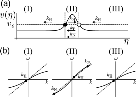
Figure 4: (a) Dependence of the probe signal velocity in the background solition’s comoving frame with spatial coordinate $\eta=x-v_{s}t$. The probe velocity is modulated by the soliton solution of the KdV equation. The horizontal dashed line indicates the soliton velocity. Two horizons are formed where the velocities of the probe and the soliton are the same, i.e., $v(\eta)=v_{s}$. The filled and open circles represent the horizons for the black and white holes, respectively. Regions I and III demarcated by the vertical dashed lines correspond to the black and white hole interiors, respectively, while region II corresponds to the exterior region between the black and white hole horizons. (b) The dispersion relation of the probe for each region is represented by the solid line in the plot. The existing modes are indicated by the intersections with the dotted line, which shows the Doppler shift. The directions of these modes are illustrated by arrows in (a), where the solid (dotted) arrow indicates the mode with a positive (negative) frequency.

Conclusion.—We have shown that (m)KdV soliton solutions exist for the circuit equations describing a TWPA transmission line comprising SNAIL elements. The soliton wave changes the velocity of a weak probe signal, describable as an effective curved space-time with analogue black hole and white hole event horizons. Suitable devices have already been experimentally demonstrated as sources of parametrically-generated multimode, entangled microwave photons. Therefore, the experimental verification of microwave analogue black hole and white hole pairs and Hawking radiation is a promising prospect. An analysis of the corresponding quantum soliton dynamics, with backreaction taken into account resulting in soliton evaporation due to Hawking radiation lasing, will be the subject of a follow-up work.