Dynamics of $\vartheta$-solitons in the HPD state of superfluid ³He-B

Abstract

In this note we present numerical study of spin dynamics of $\vartheta$-soliton in Homogeneously precessing domain (HPD) in superfluid ³He-B. The soliton consists of a small heavy core and long tails, in 1D simulation we observe their mutual motion. We also discuss mass density and tension of the soliton membrane and its 3D oscillations in a cylindrical cell.

Introduction

Spin degrees of freedom in superfluid ³He-B have spontaneously broken SO₃ symmetry [1]. State of the system can be described by a rotation matrix $R({\bf n},\vartheta)$ with axis $\bf n$ and rotation angle $\vartheta$. Spin-orbit interaction reduces the symmetry by fixing angle $\vartheta$ at value $\vartheta_{L}=\arccos(-1/4)\approx\pm 104^{\circ}$. In this system so-called $\vartheta$-solitons are possible where $\vartheta$ changes between $\vartheta_{L}$ and $2\pi-\vartheta_{L}$.

In a usual NMR experiment ³He sample is placed in constant magnetic field $H_{z}$ along $\bf\hat{z}$ axis and perpendicular radio-frequency (RF) field $H_{x}$ rotating around $H_{z}$ with angular velocity $\omega$. Depending on frequency shift $\omega-\gamma H_{z}$ and amplitude of $H_{x}$ this system can be in two states: Homogeneously-precessing domain (HPD) and Non-precessing domain (NPD) [2, 3]. $\vartheta$-solitons can exist in both states. In NPD they have only a small core where angle $\vartheta$ is changing. Size of the core is about 10..40 $\mu$m, it is determined by so-called dipolar length (ratio of gradient energy and energy of spin-orbit interaction). Analytical description of solitons in NPD is quite simple [4]. In HPD things are much more complicated. The core is surrounded by long tails where $\vartheta$ has equilibrium value, but direction of vector $\bf n$ is changing. Theoretical discussion of solitons in HPD can be found in [5]. In experiments $\vartheta$-solitons have been observed together with another type of topological defect, spin-mass vortex, in rotating ³He-B [6].

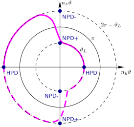
Figure 1: Schematic representation of $\vartheta$-soliton in ³He-B. See description in the text.

On Fig. 1 a schematic picture of $\vartheta$-soliton in HPD is shown in $\bf n\vartheta$ coordinates (vector with direction of $\bf n$ and absolute value of $\vartheta$). Each state of rotation matrix can be uniquely represented by a single point inside a sphere with radius $\pi$ (solid circle). Points outside the sphere can be mapped inside by adding integer number of $2\pi$ rotations to $\vartheta$. Dashed circles represent minimum of spin-orbit interaction, $\cos\vartheta=-1/4$. Points NPD+, NPD-, and HPD are equilibrium states. Without RF field HPD spontaneously breaks rotational symmetry and can exist in any point where $n_{z}=0$, $\vartheta=\vartheta_{L}$, but presence of RF pumping along $\hat{\bf x}$ stabilize HPD at $n_{y}=1$. $\vartheta$-soliton in HPD is schematically shown by thick magenta line. Dashed line is equivalent path which can be obtained from the solid line by subtracting $2\pi$ from value of $\vartheta$. For simplicity picture is drawn in $y-z$ plane, real solitons have a non-zero $n_{x}$ component.

This work is motivated by our experiments in 2017 in Helsinki (still unpublished) where we observed unexpected oscillation modes in HPD. These modes were localized in different parts of the experimental cell and had frequencies increasing with frequency shift. One of suggestions was that they are oscillations of $\vartheta$-solitons.

Numerical simulation of spin dynamics of ³He-B

Dynamics of matrix $R({\bf n},\vartheta)$ and spin $\bf S$ in superfluid ³He-B is described by Leggett equations [7]. We write them in a frame rotating around $\bf\hat{z}$ axis with angular velocity $\omega$ and solve 1D problem with only $z$-coordinate dependence:

$$\dot{\bf S} = {\bf S}\times(\gamma{\bf H}-\omega{\bf\hat{z}})$$

$$+{\bf T}^{D}+{\bf T}^{\nabla}+\mathcal{R}^{SD},$$

$${\bf\dot{n}} = -\frac{1}{2}\ {\bf n}\times\Big{[}2\,\omega{\bf\hat{z}}+\Big{(}\frac{\gamma^{2}}{\chi}{\bf S}-\gamma{\bf H}\Big{)}$$

$$+\frac{\sin\vartheta}{1-\cos\vartheta}\ {\bf n}\times\Big{(}\frac{\gamma^{2}}{\chi}{\bf S}-\gamma{\bf H}\Big{)}\Big{]},$$

$$\dot{\vartheta} = {\bf n}\cdot\Big{(}\frac{\gamma^{2}}{\chi}{\bf S}-\gamma{\bf H}\Big{)}+\mathcal{R}^{LT}.$$

Here $\gamma$ is gyromagnetic ratio of ³He, $\bf H$ is external magnetic field, $\chi$ is magnetic susceptibility. We use magnetic field which is constant in the rotating frame:

$$\gamma{\bf H}=\gamma H_{x}{\bf\hat{x}}+\gamma H_{z}{\bf\hat{z}}=\omega_{x}{\bf\hat{x}}+\omega_{z}{\bf\hat{z}},$$ (2)

and introduce frequency shift $\delta\omega=2\pi\,\delta f=\omega_{z}-\omega$.

Dipolar torque ${\bf T}^{D}$ comes from spin-orbit interaction and can be written as

$${\bf T}^{D}=\frac{4\Omega_{B}^{2}\chi}{15\gamma^{2}}\ \sin\vartheta(4\cos\vartheta+1)\ {\bf n},$$ (3)

where strength of the interaction is represented by parameter $\Omega_{B}$, Leggett frequency.

Gradient torque ${\bf T}^{\nabla}$ can be written as

$$T_{a}^{\nabla} = \frac{\chi}{\gamma^{2}}\ e_{abc}R_{cj}\Big{[}(c_{\perp}^{2}-c_{\parallel}^{2}/2)R_{bj}^{\prime\prime}$$ (4)

$$+ 2(c_{\parallel}^{2}-c_{\perp}^{2})R_{b3}^{\prime\prime}\delta_{j3}\Big{]},$$

where $c_{\parallel}$ and $c_{\perp}$ are spin-wave velocities [8], and primes are derivatives over $z$ coordinate. Expression for gradient torque via $\bf n$ and $\vartheta$ is huge, we are not writing it here.

There are two relaxation terms: spin diffusion $\mathcal{R}^{SD}$ and Leggett-Takagi relaxation $\mathcal{R}^{LT}$:

$$\mathcal{R}^{SD} = D\ {\bf S}^{\prime\prime},$$ (5)

$$\mathcal{R}^{LT} = \frac{4}{15}\ \sin\vartheta(4\cos\vartheta+1)\ \frac{1}{\tau}$$

with two additional parameters: spin diffusion coefficient $D$ and Leggett-Takagi relaxation time $\tau$. In general, spin diffusion coefficient is a tensor, but for 1D problem only a single component $D=D_{zz}$ enters the formula (see [3]).

We use PDECOL algorithm [9, 10] for integrating equations (Numerical simulation of spin dynamics of ³He-B) numerically. Original program have been written a long time ago by V.Dmitriev, we made a few modifications [11] for this work: Instead of using seven coordinates ($\bf S$, $\bf n$, and $\vartheta$) we use six, $\bf S$ and $\vartheta{\bf n}$. By doing this we avoid additional constraint $|{\bf n}|=1$, uncertainty at $\sin\vartheta=0$, and unphysical difference between ($\vartheta$, $\bf n$) and ($-\vartheta$, $-\bf n$) states. We use non-uniform adaptive mesh in the calculation, which is important because solitons have two different scales: micron-size core and millimeter-size tails. To stabilize the soliton we use exact solution for soliton core in NPD as initial conditions. It can be obtained from Leggett equations by setting all time derivatives to zero and using ${\bf n}={\bf\hat{z}}$. This leads to a differential equation:

$$\frac{12}{13}\xi_{D}^{2}\ \vartheta^{\prime\prime}=-\sin\vartheta(4\cos\vartheta+1),$$ (6)

where a conventional definition of dipolar length $\xi_{D}^{2}=\frac{65}{16}(2c_{\perp}^{2}-c_{\parallel}^{2})/\Omega_{B}^{2}$ is used. Solving it with appropriate boundary conditions we get soliton profile:

$$\vartheta=2\tan^{-1}\left[\sqrt{\frac{3}{5}}\tanh\left(\sqrt{\frac{65}{64}}\ \frac{\pm z}{\xi_{D}}\right)\right]+\pi.$$ (7)

One more problem we met in calculation was mobility of the soliton. To localize it we use a small recess in Leggett frequency profile, 5-10% decrease at $\xi_{D}$ width. Soliton with its large spin-orbit energy is pinned by this feature. By varying pinning strength we can check how this method affects calculation results. We see that there is no noticeable effect on soliton oscillation frequency and only a small change (${<}1$%) in soliton mass calculation.

We use frequency 1.124 MHz, and cell length 0.9 cm, same as we had in the experiment. The soliton is created in the middle of the cell and stabilized by waiting long enough time, changing relaxation terms, or doing averaging of motion over some time and using result as new initial conditions. Starting from a stable state with the soliton we excite oscillations by a small change of frequency shift (which is equivalent to a small step in static magnetic field) and record components of integral magnetization. Fourier spectrum of magnetization is fitted using a model signal which is sum of a few decaying harmonic oscillations. We observed both oscillations of the soliton and uniform HPD oscillations [12]. Frequency of uniform oscillations is known, it can be used as an additional check of calculation accuracy:

$$\Omega^{2}=\frac{4}{\sqrt{15}}\ \frac{\omega_{x}\omega\,\Omega_{B}^{2}}{\omega^{2}+8/3\,\Omega_{B}^{2}}.$$ (8)

With this excitation method we usually observe two first modes of soliton oscillations. Third and forth modes are much weaker and can be seen only at some conditions.

Results

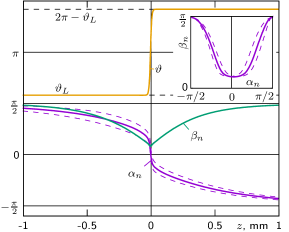
Figure 2: Soliton profile: angle $\vartheta$, polar ($\beta_{n}$) and azimuthal ($\alpha_{n}$) angles of $\bf n$ vs. coordinate $z$. Dashed color lines near $\alpha_{n}$ profile show main mode of soliton oscillations. Inset: $\beta_{n}$ vs. $\alpha_{n}$ plot. The figure is calculated with $c_{\perp}=1115$ cm/s, $\Omega_{B}/2\pi=235.8$ Hz (which corresponds to $T=0.6~{}Tc,P=25.7$ bar), $D=0.01$ cm²/s, no Leggett-Takagi relaxation, $H_{x}=4$ mG, frequency shift $\delta f$ = 40 Hz.

On Fig. 2 an example of soliton equilibrium profile is shown. Direction of vector $\bf n$ is represented by polar and azimuthal angles, $\beta_{n}$, and $\alpha_{n}$. One can see a small core where angle $\vartheta$ changes between equilibrium values $\vartheta_{L}$ and $2\pi-\vartheta_{L}$ at distance $\sim 10\mu$m and tails where $\bf n$ is rotated at distance $\sim 1$ mm. It’s interesting to see that soliton tails are slightly asymmetric (they go towards different states, NPD+ and NPD- ), and that in the center vector $\bf n$ does not reach vertical position as it was suggested in [5]. Soliton core is not just change of $\vartheta$, it also includes rotation of $\bf n$ by some noticeable angle. Main mode of soliton oscillations is shown by dashed color lines. In this mode the soliton tail is rotating around vertical axis, only azimuthal angle $\alpha_{n}$ is changing.

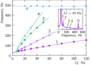
Figure 3: Oscillation frequencies as a function of frequency shift. Calculation is done for $\Omega_{B}/2\pi=100$ kHz, $c_{\perp}=1000$ cm/s, $H_{x}=8$ mG. One can see four soliton oscillation modes (labeled “1”..“4”) and HPD uniform mode (labeled “U”). Inset shows an example of magnetization spectrum at frequency shift $\delta f=40$ Hz. Lines are fits to formula (9) with free parameters $B$ and $C$.

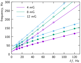
Figure 4: Frequencies of soliton modes 1 and 2 as a function of frequency shift for three different values of RF pumping: 4 mG (magenta points), 8 mG (green points), 12 mG (blue points). Calculation is done for $T=0.6\,T_{c}$, $P=25.7$ bar ($\Omega_{B}/2\pi=235.8$ kHz, $c_{\perp}=1115$ cm/s). Lines are drawn using approximation formulas (9) and (10).

On Fig. 3 oscillation frequencies are shown as a a function of frequency shift. The highest, shift-independent mode is uniform HPD oscillations (8), others are oscillations of the soliton. We found that frequencies of all soliton modes as a function of frequency shift $\delta\omega$ can be written as:

$$\Omega^{2} = B\,\omega(\delta\omega\pm\omega_{x}/\sqrt{15})+C\,\delta\omega^{2}$$ (9)

with “$+$” sign for modes 1, 2 and “$-$” for modes 3, 4. There is no exact theory behind this formula, it’s just an approximation which works for all observed modes. Note that ratio $\sqrt{15}$ between RF pumping and frequency shift is special for HPD: at $\delta\omega<\omega_{x}/\sqrt{15}$ uniform HPD state becomes unstable. Parameters $B$ and $C$ depend only on RF pumping amplitude $\omega_{x}$ and Leggett frequency $\Omega_{B}$. Me have measured modes 1 and 2 for $P=25.7$ bar, $T=0.6\ldots 0.9T_{c}$, $H_{x}=4\ldots 12$ mG and found approximation formulas (see Fig. 4):

$$B_{1,2} = \sqrt{\frac{\omega_{x}}{\omega}}\left(\frac{1}{107}+372\frac{\omega_{x}}{\omega}\right),$$ (10)

$$C_{1} = 0.278+27.4\sqrt{\frac{\omega_{x}}{\Omega_{B}}}\left(1+0.04\frac{\omega}{\Omega_{B}}\right),$$

$$C_{2} = 1.16+319\sqrt{\frac{\omega_{x}}{\Omega_{B}}}\left(1+0.08\frac{\omega}{\Omega_{B}}\right).$$

We also found that relaxation of soliton oscillations is determined by spin diffusion, but not Leggett-Takagi relaxation.

Oscillation of a soliton membrane

Let’s calculate mass density, associated with a soliton. First we solve second and third Leggett equations (Numerical simulation of spin dynamics of ³He-B) for spin:

$$\frac{\gamma^{2}}{\chi}{\bf S} = \gamma{\bf H}+{\bf n}\ \dot{\vartheta}$$

$$+ (1-\cos\vartheta)\ {\bf n}\times({\bf\dot{n}}+{\bf n}\times\omega{\bf\hat{z}})$$

$$+ \sin\vartheta\ ({\bf\dot{n}}+{\bf n}\times\omega{\bf\hat{z}}).$$

From this formula one can see how spin is created by magnetic field and by motion of ${\bf n}$ and $\vartheta$. There are also terms with $\omega$ which come from rotation of the frame. Consider a soliton which is moving with velocity $v$ along ${\bf\hat{z}}$ axis. We can write ${\bf\dot{n}}=\frac{d}{dt}{\bf n}(z+v\,dt)=v\,{\bf n}^{\prime}$, and same for $\vartheta$. Using formula (Oscillation of a soliton membrane) we can find spin created by soliton motion. Energy associated with spin is $F=\frac{\gamma^{2}}{2\chi}{\bf S}^{2}-({\bf S}\cdot\gamma{\bf H})$. Term proportional to $v^{2}$ will give us mass density of the soliton:

$$m=\frac{\chi}{\gamma^{2}}\left[(\vartheta^{\prime})^{2}+2(1-\cos\vartheta)\ ({\bf n^{\prime}})^{2}\right]$$ (12)

In this discussion we assumed that moving soliton have same profile as stationary one. This is true for small velocities. Formula for a soliton moving with arbitrary velocity can be found in [13].

Figure 5: Mass profile of a soliton. Total mass is split into two parts, corresponding to two terms of (12). Calculated with same parameters as Fig. 2.

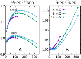
Figure 6: A: Ratio of soliton mass in HPD (total mass and mass of the core) and in NPD as a function of frequency shift, for three different values of RF pumping: 4 mG (magenta points), 8 mG (green points), 12 mG (blue points). B: Ratio of wave velocity $C$ for soliton in HPD and in NPD.

Consider a $\vartheta$-soliton in NPD (6-7) pinned to walls of a cylindrical cell perpendicular to cell axis. It can move as a circular membrane. We can find mass $M$ of unit area by integrating (12) along $\bf\hat{z}$ axis. We calculate tension $T$ of the membrane as total potential energy (gradient and spin-orbit) of the soliton per unit area. We ignore additional gradient forces which come from bending of the soliton because they are small if cell size is bigger then soliton thickness. Using soliton profile (7) we obtain

$$M=\frac{13}{3}\frac{\chi}{\gamma^{2}\xi_{D}^{2}}\int_{-\infty}^{+\infty}\Big{(}\cos\vartheta(z)+\frac{1}{4}\Big{)}^{2}dz,$$ (13)

$$T=\frac{16}{15}\frac{\chi\Omega_{B}^{2}}{\gamma^{2}}\int_{-\infty}^{+\infty}\Big{(}\cos\vartheta(z)+\frac{1}{4}\Big{)}^{2}dz.$$ (14)

Ratio of tension and mass give square of wave velocity $C$ along the membrane,

$$C^{2}=2c_{\perp}^{2}-c_{\parallel}^{2}.$$ (15)

Oscillation frequencies of the membrane are determined by zeros of Bessel functions, the first one for membrane radius $r$ is $2.405\,C/r$. For $T=0.6~{}T_{c}$, $P=25.7$ bar, and $r=3.9$ mm this gives 1.7 kHz.

In numerical simulation we can find mass and tension of the soliton in HPD and compare it with NPD case. It is also possible to separate masses of tail and core of the soliton. On Fig. 5 example of mass density of a soliton in HPD is presented. Mass is splitted into two parts which correspond to two terms in (12): $m_{\vartheta}$ comes from motion of $\vartheta$, and $m_{\bf n}$ is created by motion of $\bf n$. On Fig. 6 calculated mass and wave velocity of soliton in HPD is compared with values for soliton in NPD (formulas 13 and 15).

Conclusions

Homogeneously precessing domain is a well-defined system which can be used as a sensitive tool for studying ³He properties. Understanding of topological defects in this system should be important for future experiments. In this work we developed numerical simulation of $\theta$-solitons in HPD. We observed a few oscillation modes of soliton tails with respect to its core. We also discuss 3D oscillations of the soliton membrane pinned to walls in both HPD and NPD. One can imagine other oscillation modes in this system, for example non-uniform motion of tails in the plane of the soliton.

We think that further theoretical, numerical, and experimental investigation of $\theta$-solitons in HPD is needed. It is still not clear what is reliable way of producing solitons in experiment, and were oscillation modes observed in experiments mentioned above related to solitons.

References

- [1] D. Vollhardt and P. Wölfle “The superfluid phases of helium 3” TaylorFrancis, London, 1990
- [2] A.S. Borovik-Romanov et al. “Experimental study of separation of magnetization precession in 3He-B into two magnetic domains” In JETP 61, 1985, pp. 1199–1206 URL: http://inis.iaea.org/search/search.aspx?orig_q=RN:18003987
- [3] I.A. Fomin “Separation of magnetization precession in 3He-B into two magnetic domains. Theory” In JETP 61, 1985, pp. 1207–1213 URL: https://doi.org/10.1142/9789814317344_0036
- [4] Kazumi Maki and Pradeep Kumar “Magnetic solitons in superfluid ” In Phys. Rev. B 14 American Physical Society, 1976, pp. 118–127 DOI: 10.1103/PhysRevB.14.118
- [5] T. Sh. Misirpashaev and G.E. Volovik “Topology of coherent precession in superfluid 3He-B” In JETP 75, 1992, pp. 650–665 URL: http://inis.iaea.org/search/search.aspx?orig_q=RN:24044181
- [6] Y. Kondo et al. “Combined spin-mass vortex with soliton tail in superfluid 3He-B” In Phys. Rev. Lett. 68 American Physical Society, 1992, pp. 3331–3334 DOI: 10.1103/PhysRevLett.68.3331
- [7] Anthony J. Leggett “A theoretical description of the new phases of liquid 3He” In Rev. Mod. Phys. 47 American Physical Society, 1975, pp. 331–414 DOI: 10.1103/RevModPhys.47.331
- [8] V. V. Zavjalov, S. Autti, V. B. Eltsov and P. J. Heikkinen “Measurements of the anisotropic mass of magnons confined in a harmonic trap in superfluid 3He-B” In JETP Letters 101.12, 2015, pp. 802–807 DOI: 10.1134/S0021364015120152
- [9] N. K. Madsen and R. F. Sincovec “Algorithm 540: PDECOL, General Collocation Software for Partial Differential Equations [D3]” In ACM Trans. Math. Softw. 5.3 New York, NY, USA: Association for Computing Machinery, 1979, pp. 326351 DOI: 10.1145/355841.355849
- [10] Tim Hopkins “Remark on Algorithm 540” In ACM Trans. Math. Softw. 18.3 New York, NY, USA: Association for Computing Machinery, 1992, pp. 343344 DOI: 10.1145/131766.131773
- [11] , https://github.com/slazav/he3vmcw
- [12] V.V. Dmitriev, V.V. Zavjalov and D.Ye. Zmeev “Spatially homogeneous oscillations of homogeneously precessing domain in 3He-B” 10.1007/s10909-005-2300-5 In Journal of Low Temperature Physics 138 Springer Netherlands, 2005, pp. 765–770 URL: http://doi.org/10.1007/s10909-005-2300-5
- [13] S. S. Rozhkov “Dynamics of the order parameter of superfluid phases of helium-3” In Soviet Physics Uspekhi 29.2 IOP Publishing, 1986, pp. 186–198 DOI: 10.1070/pu1986v029n02abeh003163